Agents on a Landscape: Simulating Spatial and Temporal Interactions in Economic and Ecological Systems

1 Introduction

Today, the tremendous value of ecosystem services is widely recognized among social and environmental scientists. Scholars have developed a suite of tools focused on estimating the value of ecosystem services ranging from carbon sequestration to pollination (Costanza et al., 2014; Turner et al., 2016; Johnson et al., 2021). These models provide important estimates on the value of nature to humanity and offer essential guidance to policymakers seeking to achieve sustainable development goals. But some ecosystem services are more challenging to model than others. The harvesting of nontimber forest products (NTFP), for example, requires that we consider not only spatial heterogeneity, but also inter-agent competition.

Unfortunately, many models of human resource allocations, such as standard models in economics, fall short in their ability to convey these critical components. Economics models have been successfully expanded to incorporate geographic, social, or other conceptions of space (Chael et al., 2019; Glenk et al., 2020; Graubner et al., 2021). But with respect to NTFP harvesting, a model must factor in space and inter-agent competition, and here we find that standard economics approaches often fall short.

In this paper, we extend the standard economic model of the representative agent to an agent-based simulation that predicts firewood harvesting and the value of harvesting to agents. Our approach uses agent-based simulation (ABS), a method widely used in the life sciences to convey phenomena such as wildlife movement (Blackwell, 1997; Patterson et al., 2008; Kranstauber et al., 2012). Past research has also used ABS to evaluate interactions between human and ecological systems (Hare and Deadman, 2004; Schreinemachers and Berger, 2011; Le et al., 2012; Huber et al., 2018; Dou et al., 2020). We define a model consisting of millions of agents, defined spatially, who can influence each other’s set of potential payoffs as they maximize their respective utility. Specifically, we modify a well-known economic household consumption and production model from Bardhan and Udry (1999) and show how interacting agents and spatially-explicit information modifies the production and utility functions. An important contribution of this paper is that we explicitly map the agent-based simulation rules to the corresponding functions, maximizations and definitions of equilibrium typical to the standard economics model, illustrating that these two approaches can be merged and are complementary (so long as one takes an iterative approach to finding equilibrium). And by conducting a simulation, we can incorporate non-cooperative behavior and spatial heterogeneity of natural capital availability directly into our framework. We use our model and data from Tanzania to predict the location of firewood extraction, the amounts of firewood consumed, and the value of this firewood to households.

Since Hotelling (1929), economists have been aware of the importance of space and distance for particular conceptual frameworks. This effort was further advanced by the development of the widely used Sugarscape Model, which simulates agent interactions to study phenomena such as group formation (Epstein and Axtell, 1996). In recent years, there have been several important efforts to directly incorporate spatial heterogeneity into models of human–ecosystem interactions (Albers and Robinson, 2013). Previous studies often use static household production and consumption models that do not account for the repeated activities of agents over time or competition among agents (Sterner et al., 2018). Moreover, most existing spatially explicit models from economic theory operationalize resource proximity based on one-dimensional access to a homogenous stock of natural capital. Agents, however, operate in at least two dimensions as they navigate landscapes over which natural capital resource availability varies considerably.

Our model places both agents and NTFP goods on a high-resolution landscape of grid-cells, where agents must move over a non-uniform landscape characterized by terrain and road networks to gather goods. The corresponding ABS accounts for the unique configuration of the landscape by using relatively high resolution data inputs (here, 500 m) and generates results at an equally high resolution. We also developed the simulation such that it can accommodate large numbers of agents.

Modeling many agents at a high resolution is computationally challenging, so we also present computational methods capable of efficient simulation at this scale in the Supplementary Material section. Specifically, the advances include an efficient route-finding algorithm used to estimate agent traversal times (Supplementary Section 3), as well as the creation of a customized simulation environment that vectorizes all computation in multi-dimensional arrays to allow for efficient computation (Supplementary Section 6) rather than using a generalized simulation environment (such as NetLogo or other tools commonly used for ABS). These advancements align with recent innovations that improve on the efficiency of stochastic simulations in fields such as chemistry, biology, and ecology (Gillespie, 1977; Cao et al., 2006; Black and McKane, 2012; Wilkinson, 2019; Oraby et al., 2021).

This work contributes to economic discourses on renewable resources and household NTFP extraction.¹ We build on several recent works in spatial natural resource economics. For example, Miteva et al. (2017) and Bošković et al. (2018) develop household decision models in which households differ in their ability to reach the forest and (in Miteva et al., 2017) the market. These models predict household consumption, collection, buying, and selling patterns of NTFP given heterogeneous market and forest proximity. Our study expands on this work by defining resource availability based on a two-dimensional grid instead of a binary, one-dimensional indicator. Our work is also complementary to this previous research, which seeks to understand who extracts. In addition to who, our model helps us determine where extraction happens.

To account for non-cooperative behavior among agents, Sterner et al. (2018) use a game theory approach based on sorting models to evaluate possible locations of natural resource extraction at equilibrium. Like Sterner et al. (2018), we incorporate non-cooperative behavior among agents by factoring in NTFP depletion over time, which forces other agents to search elsewhere. The simulation component of our paper builds on this work, as we can incorporate repeated actions of agents competing for resources over landscapes over which the distribution of resources is not homogeneous.

This paper proceeds as follows. In Section 2.1, we describe the general modeling framework, including how we define the agent, the passage of time, behavior rules and the definition of equilibrium in this type of model. Section 2.2 reviews the data used for the empirical application of the model with emphasis on how data can be created for any location on the globe. Section 3 provides detailed results on foraging behavior in Tanzania, as well as a sensitivity analysis. We offer concluding remarks in Section 4.

2 Materials and Methods

2.1 Model

The foraging model presented in this section defines the elements that comprise our simulation model. These include the landscape network, the passage of time, and the agent and behavior rules. This section describes each of these parts of the general model and incorporates examples from NTFP collection in Tanzania to illustrate the importance of each element. Given the complexity of our simulation, we organize information about our model in an ODD+D protocol in Supplementary Section 7 (Grimm et al., 2020).

2.1.1 Behavior Rules: Household Production and Utility Maximization

Our approach builds on traditional agricultural household models used extensively in development economics (Singh et al., 1986, Bardhan and Udry, 1999). Each agent chooses to allocate their full labor time to leisure, foraging or wage work. The agent maximizes their utility in time period t by choosing to allocate their labor to gathering firewood, a wage generating activity (that yields income to purchase a firewood substitute) or leisure. Their choice is constrained by the foraging production possibilities, a budget constraint, and the amount of labor they have available to allocate on each activity. The utility maximization problem facing each agent i is therefore as follows:

$$\begin{array}{cc}\hfill \text{Max}& u_i(c_i,L_i^l)={\text{α}}_i{c}_i^{{\text{β}}_i^c}{L}_i^l{}_{}^{{\text{β}}_i^l}\hfill \\ \hfill Subjectto:& L_i^g+L_i^w+L_i^l\le L\hfill \\ \hfill & g_i=f\left(L_i^g\right|N_i,R_{j\in \sim i})\hfill \\ \hfill & c_i=c_i^g+c_i^b-c_i^s\hfill \\ \hfill & g_i=c_i^g+c_i^s\hfill \\ \hfill & p_b{c}_i^b=p_w{L}_i^w+p_s{c}_i^s\hfill \end{array}$$

The agent’s utility u_i is a function of their consumption of cooking fuel c_i and non-labor (leisure) time $L_i^l.$We use a Cobb-Douglass functional form with constant scalar α_i and parameters ${\mathrm{\beta }}_i^c+{\mathrm{\beta }}_i^l=1$. This functional form is well suited for our model. Our agent values consumption of both goods but will experience diminishing marginal utility as they consume more and more of one good at the expense of the other. The Cobb–Douglas utility function captures these important characteristics of the agent’s preferences. Moreover, the exponential parameters reflect the agent’s relative preferences over the two goods: for example, if the agent prefers fuelwood over leisure, then ${\mathrm{\beta }}_i^c>{\mathrm{\beta }}_i^l.$

The agent has finite resources to allocate towards consuming these two goods. Each agent is endowed with labor L, which they may allocate to gathering a spatially defined good ($L_i^g)$, to wage work, ($L_i^w)$ and to leisure$(L_i^l)$. The agent can use an allocation of their labor ($L_i^g)$ to collect firewood, producing the gathered good g_i. The agent’s production of g_i is affected by the agent’s location on a landscape, N_i, as well as the gathering actions of other agents, R_j∈i. This is one of the ways in which our approach builds on previous household models, as the production function is determined by the spatially heterogeneous distribution networks of firewood stocks that are unique to each agent and the actions of rival agents to change the production function.

Once produced, the gathered good can either be consumed ($c_i^g$) or sold ($c_i^s)$. Agents may purchase cooking fuel in the market as an alternative or supplement to their gathering behavior, such that total consumption of the gathered good, c_i, is the sum of $c_i^g$ and the quantity of cooking fuel purchased from the market, $c_i^b$. Please note that the cooking fuel that our agent encounters in the market is an energy source that is not harvested from the forest, such as kerosene. The purchased good is bought at price p_b from the money income of the agent. Income is earned either by selling the gathered good at price p_s or working for wages at price p_w.

We simplify the model further by assuming that agents do not sell any of the firewood they have gathered due to transport costs and distance to markets so that p_s = 0 and $c_i^s$ = 0. As discussed in the Introduction, the assumption that agents do not sell the firewood they collect holds quite broadly in Tanzania, the case study we use in this paper (Faße and Grote, 2013). And under this simplification of the model, agents may still purchase a firewood substitute from markets. Additionally, we assume that agents spend their full budget each time period and all of the endowed labor is allocated to one of the three possible choices. With these assumptions, we can simply the agent’s maximization problem to the following:

$$\begin{array}{cc}\hfill Max& {\text{α}}_{\mathit{i }}{\mathbf{\left(}\mathit{f }\right(L_i^g|N_i,R_{j\in \sim i})+\mathbf{\left(}\frac{p_w}{p_b}\mathbf{\right)}{L}_i^w\mathbf{)}}^{{\text{β}}_i^c}{L}_i^l{}_{}^{{\text{β}}_i^l}\hfill \\ \hfill Subjectto:& L_i^g+L_i^w+L_i^l\le L\hfill \end{array}$$

The full profit function the individual faces combines the wages they receive and the firewood they gathered, valued at the price of the firewood substitute (the market-purchased cooking fuel):

$${\mathrm{\Pi }}^{*}(p_w,p_b,L)=p_b\mathit{f }\left(L_i^g|N_i,R_{j\in \sim i}\right)+p_w{L}_i^w$$

Figure 1 graphs one example agent’s labor allocation choice and specifies an example production function, profit function and a utility indifference curve at the optimized labor allocation choice. In this case, the individual forages for most of their fuel needs ($g_i^{*}$) but supplements firewood with purchased fuel ($c_i^b{}^{*}$), shown as quantities on the vertical axis. The labor decisions made by this agent are shown on the horizontal axis. Note that the horizontal axis also plots the negative value of leisure so that utility is represented with a flipped indifference curve between the gathered good and leisure.

FIGURE 1

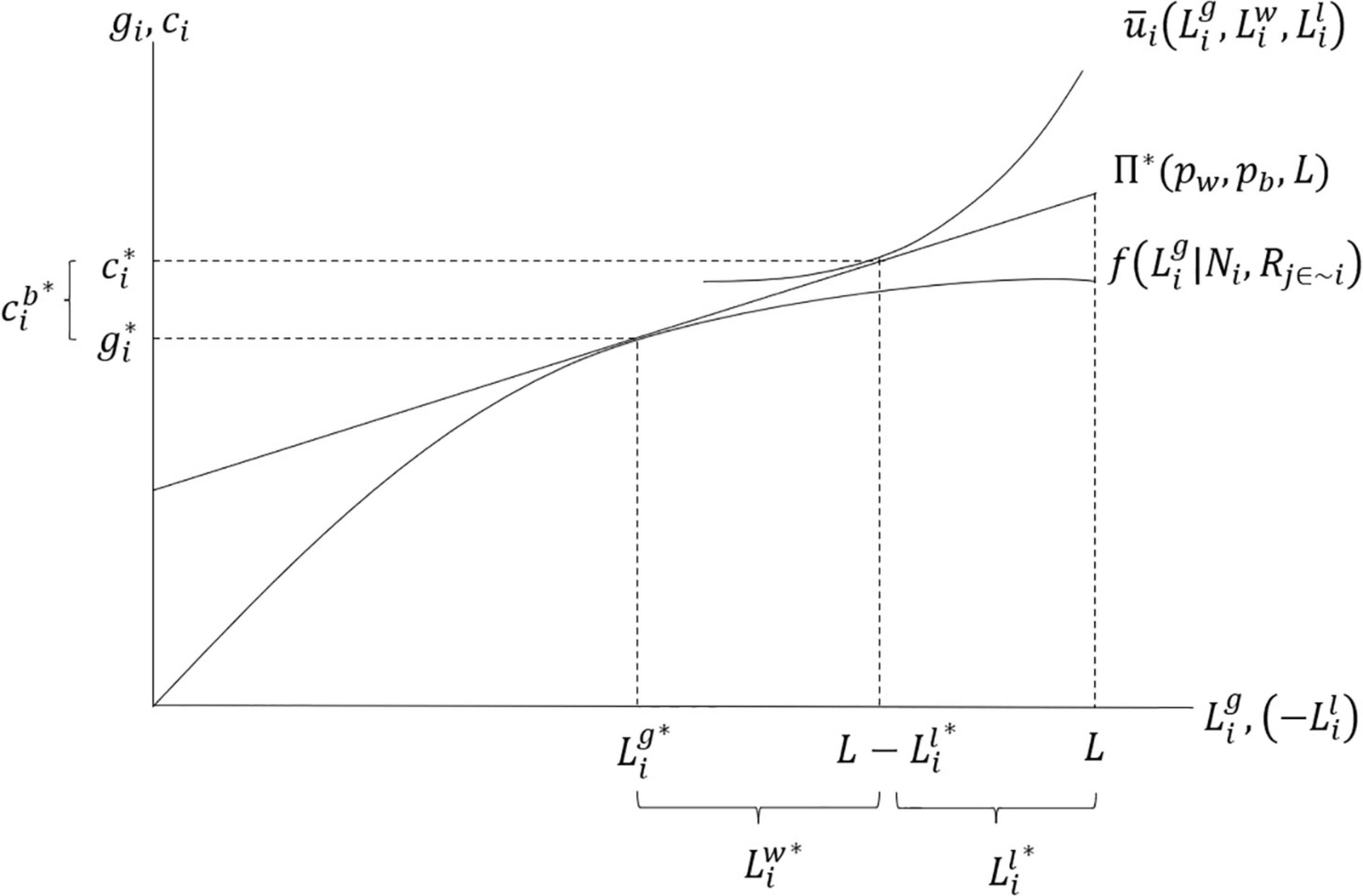
Figure 1. Conceptual model of household production and consumption decisions. Note: The asterisk indicates that the time allocations maximize household utility (welfare).

2.1.2 The Landscape Grid

We enhance the household model by defining a gridded landscape that captures variation in natural capital stocks over two-dimensional space. Our approach is similar to modeling methods in studies from fields such as transportation and civil engineering (see Rodrigue, 2020 for an overview), physics (Barthélemy, 2011), fishery management (Rassweiler et al., 2012), and ecology (Kool et al., 2013). Our grid cells are defined at a 500 m resolution, and each grid-cell is characterized by a travel network (defined from road, river, terrain, and other inputs), the abundance of firewood, and the predicted wage. We describe how we derive these estimates for each grid-cell in Section 2.2.

In our model, we assume that agents have complete information over the firewood stocks in each grid-cell over the landscape grid. For our model, this assumption is appropriate because, as we discuss in Section 2.2.2, each agent’s choices represent the choices of all people living in the agent’s village. In this sense, our agent represents a group of people who likely share collective knowledge of all natural capital stocks nearby. Future extensions of our model could certainly add imperfect or asymmetric information, if such additions were important for the goals of the analysis.

Because agents have complete information, they do not incur penalties from changing their foraging strategy.

2.1.3 Two Conceptions of Time

Throughout this analysis, we refer to the passage of time with two different concepts: the iteration step (subscripted s) and the time period shown in the household model (subscripted t). One time period is composed of many iteration steps. The reason for this differentiation is to distinguish between the actual passage of time and the iteration method used to make the simulation possible. Within this framework, the resource stock in each cell can change in two ways. First, changes may occur when transitioning from time t to t + 1. These shifts reflect changes that occur independent of the activities of agents, such as the regrowth of trees. The resource stock can also change as the result of an agent action at time s (e.g., harvesting the dead wood in the cell, planting a crop, etc.).

Additionally, we define the action order, a list of agents ordered by when they can make an action relative to other agents. During each time period, the first agent in the action order makes one action in step s, followed by the second agent in the action order in step s+1. This process continues with new steps until the end of the action order list is reached, at which point the simulation loops through the agents again. We repeat this until no valid agent actions remain.

Having a time-step smaller than the full time period is necessary to simulate agent competition and also is a mechanism to increase fidelity of the simulation. It is possible that biases arise based on how the action order is defined, but in most cases the bias approaches zero as the size of the step decreases. For example, if we define an action order in which agents may forage firewood from a forest and we choose a large step size in which each agent is allowed to satisfy their full demand on their first action, then the results will be very sensitive to the order in which actions happen. However, if we limit the amount an agent can forage during each step to ever smaller quantities, the results become less sensitive to the initial ordering.

If we only define the action order once for all time periods, the predictions will be biased, as agent outcomes will largely be a function of the order in which they took their actions. Past ABS approaches have randomly assigned agent waiting times between events to overcome this source of bias (Lehman et al., 2012). We reduce bias by re-generating the action order for each time period. That’s to say, at the start of each time period t, the action order is randomized anew, which reduces the bias in our results, since no agent will move early in every time period.

We denote the two conceptions of time with sets S and T. Set S contains the action order and the definition of what may be done within one iteration step. Set T assumes time progresses from t=1 to t=T and includes the full set of the landscape changes between time periods that are exogenous to agent actions (such as forest regrowth). Our model assumes that the landscape grid of firewood stock fully regenerates between each time period. Future extensions of this model could draw on insights from the forestry literature to augment the characterization of firewood regeneration.

2.1.4 The Agent

As mentioned, agents in our simulation have full information on the NTFP stocks in nearby grid-cells. The set of agents, A, is described by an attribute table consisting of an agent identity column (unique for each agent) and corresponding columns of agent attributes. This data type is different from the cell networks because the agent identity is not tied to a fixed location as it is for a cell. Rather, the cell network is a space through which agents move.

Although agents do not have fixed locations, agent locations and attributes can be aggregated, at a given time and step, to create a matrix that describes a static moment (this process is at the heart of the computational methods used in the simulation). For each agent, a_i∈I, the agent attribute table must denote the agent’s geographic location at every time period and iteration step defined in reference to a cell within a valid geospatial cell network and steps within the time structure. Although we do not do so for our study, the agent attribute table could be expanded to include important agent characteristics, such as agent-level demographic indicators, current assets, other location references like work location and house location, or relationship status with other agents.

We now consider the addition of spatially heterogeneous production and competition. Consider first the production decisions an agent faces when on a heterogeneous landscape but while temporarily assuming there are no competing agents. Above, we denoted the production function as subject to a term N_i that represents the gridded landscape as viewed from the ith position. Two key matrices in this set are the firewood abundance matrix and the net-profit matrix. Net profit depends both on how much firewood is present in each grid-cell and the travel costs incurred getting to that cell from the center of the matrix. We define net profit more precisely in Section 2.2.

The agent follows a max-marginal-gain set of behavior rules that specifies how the agent considers the marginal gain they would get from expending one step’s worth of labor on each of the possible labor choices. The agent then does whichever action maximizes this gain. For example, if the marginal gain from foraging is higher than from wage work or leisure, then the agent will spend the full simulation step foraging (note that simulation steps will be defined sufficiently small such that this assumption does not affect the results). If the agent still has available labor after foraging from one grid-cell, they may spend it on another action, continuing until the labor they have in the current step is depleted.

Figure 2 provides a hypothetical example to help illustrate the process of agent foraging in our model. Please note that in the actual model, the amount an agent harvests per iteration step will be much smaller and grid-cells will only be exhausted of their firewood stock once multiple agents have foraged on them. For this illustration, the upper-right corner shows an example net profit matrix. In this example, there is a high-quality forest in the northwest and a lower-quality forest in the southeast. In both cases, the forests have diminishing net profit available on the sides furthest from the center of the matrix (the agent’s location) because foraging from these cells will incur additional travel costs. When it is the i^th agent’s iteration step, the max-marginal-gain behavioral rule discussed above implies that the agent will gather from grid-cell N_1,1 where the net profit is 6. After a cell has been foraged, assume its remaining value is zero. Assume further that the step-size in this example is defined so that an agent may only deplete one grid-cell per step. Thus, in this case, the agent gets a marginal value on this step equal to 6. This value is plotted in the blue line, which represents the marginal product of foraging, and also the orange line, which represents the production function. On the agent’s next turn, they will choose to forage either on N_0,1orN_1,0, will gain a marginal value equal to 5, and will increase total production to 11. This process will iteratively continue, one action per iteration step, until the agent has no remaining grid-cells with positive net profit.

FIGURE 2

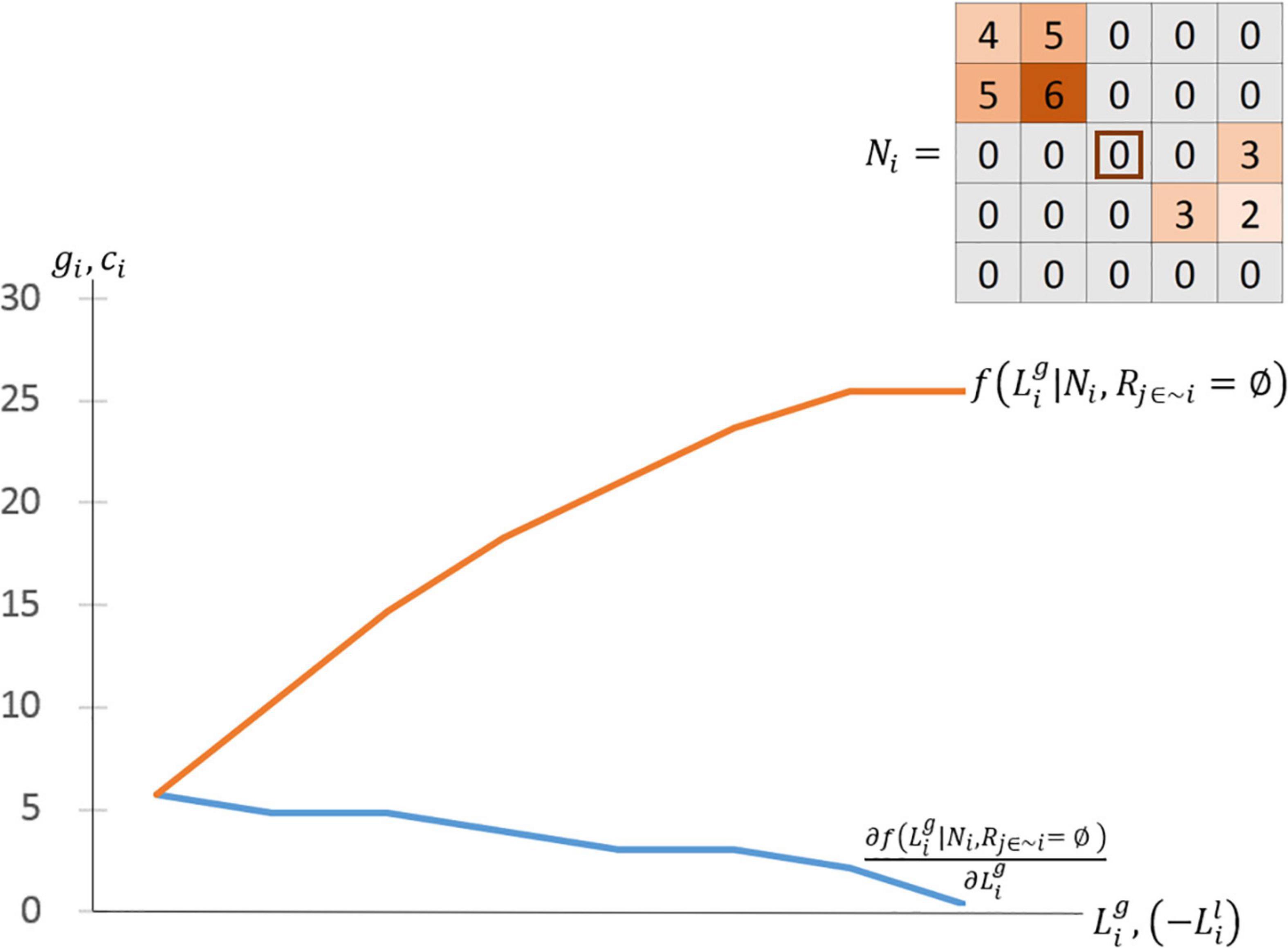
Figure 2. Generating a production function from a net profit geospatial grid-cell matrix given no competition.

Our production function ignores the non-production activities the agent may do. At each iteration step in the full decision framework, the agent chooses to allocate labor to $L_i^g,L_i^w,or{L}_i^l$, based on whichever has the highest marginal value. The marginal value from $L_i^g$ is derived from N_i as described above, while the marginal values from leisure and purchased fuel depend on the shape of the agent’s utility function and the prices of wage labor and fuel. Given concave production and concave utility from leisure, this means in the initial iteration steps of a time period, the agent will alternate between producing firewood and enjoying leisure. Eventually, diminishing returns will cause the agent to switch to wage labor for the final units of fuel consumed. This process is depicted in Figure 3, where each blue arrow indicates the action chosen on the sth iteration step.

FIGURE 3

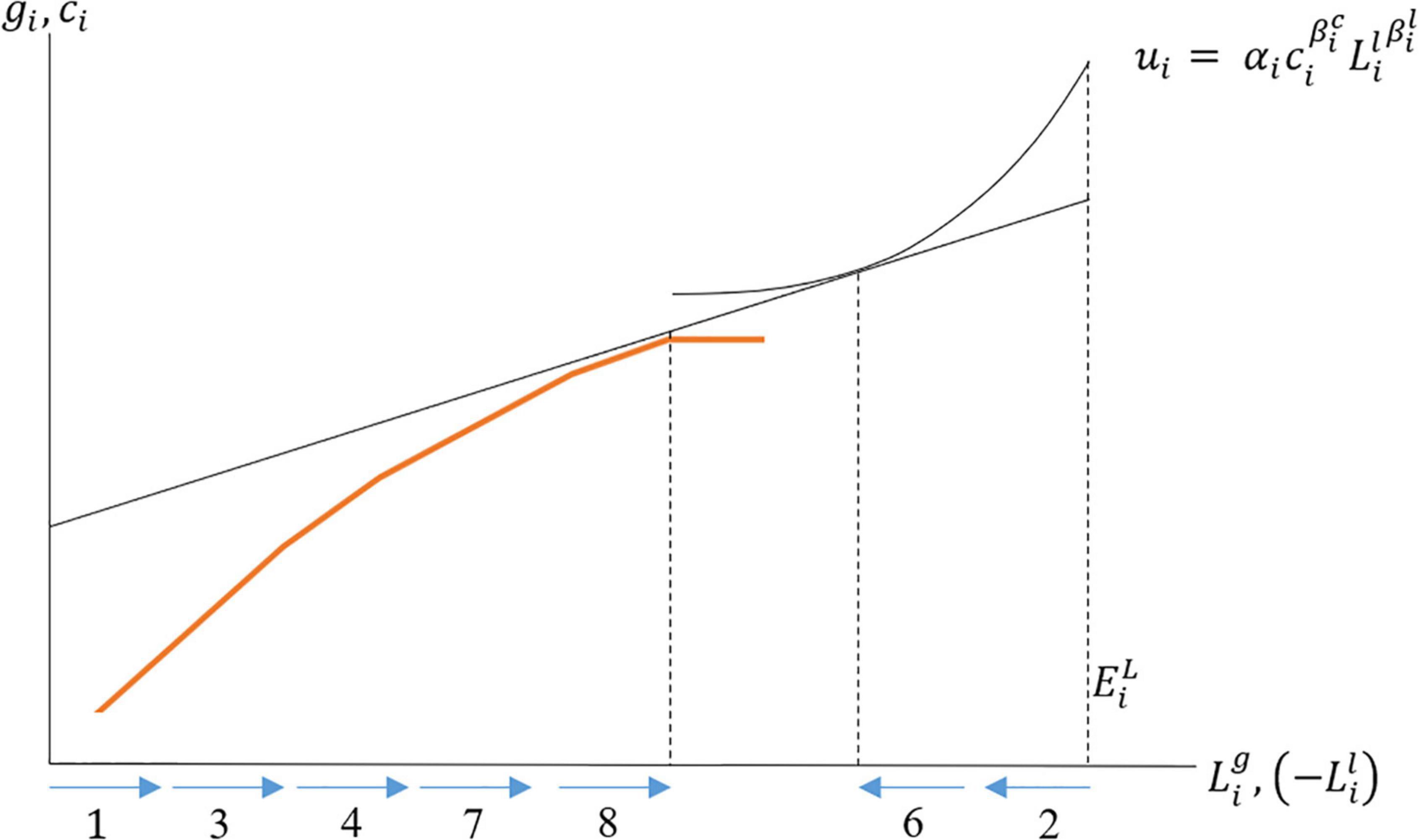
Figure 3. Max-marginal-gain choices between leisure, production, and wage earnings over multiple iteration steps.

The iterative process by which the agent moves towards the maximized point allows for events to happen in between each decision step the agent takes. The main type of inter-step event we include is depletion of the forest by other agents. The production function and corresponding iterative solution method defined above assumed no competing agents were present. Below, we extend this to multiple agents.

Situations in which agents engage in strategic interdependence may lead the max-marginal-gain decision rule to suboptimal allocations. For instance, agent 1 may have predicted that agent 2 would want to forage from the contested cell and would thus choose to forage there earlier. This type of strategic behavior can easily be included in agent simulation by using modified decision rules (such as doing the best-response action in a Nash equilibrium). But in many applications, this becomes computationally impossible when millions of agents are considered simultaneously and does not present large deviations from the naïve max-marginal-gain decision rule. Thus, we assume there is no strategic interdependence between agents.

We solve the model iteratively, allowing each agent at each iteration step to make their utility maximizing choice. Throughout our model, competition between agents occurs implicitly, as the private actions of each agent influence other agents’ access to firewood.

2.1.5 Definition of Equilibrium

The results of our simulation are compatible with the underlying economic theory and can be expressed as inter-temporal and intra-temporal equilibria. Because the application used in this section focuses on sustainable harvest rates, we focus on the intra-temporal equilibrium, using a conception similar to the Ramsey (1928) approach.

To define equilibrium, first define zero-profit zones for each agent B_i = {N_i ∀ i where f_i (N_i, R_j∈i = ∅) > 0}. The zero-profit boundary B_i is the set of all grid-cells where the agent has positive net-profit assuming no other agents deplete the grid-cells and assuming the agent spends their entire endowment of labor on foraging. Outside the zero-profit boundary, the agent has no profitable cells even in the best circumstances, so ignoring these cells has no impact on the outcome.

An intra-temporal equilibrium is characterized by allocation choices of labor $(L_i^g,L_i^w,L_i^l)\forall i\in A$ and a geospatial grid-cell matrix of local prices P_k for each kth good such that each agent satisfies the following conditions:

1. There does not exist any grid-cell within the ith agent’s zero-profit zone B_i where $U_{\mathit{i }}\left(N_{\mathit{i }}\left(netprofit\right)\right)>U_{\mathit{i }}\left(L_i^l\right)$.

2. There does not exist any possible purchase where $U_{\mathit{i }}\left(\left(\frac{p_w}{p_b}\right){\mathit{ L}}_i^w\right)>U_{\mathit{i }}\left(L_i^l\right)$.

Although we have specified this model so that it is based only on one good (produced two ways) and leisure chosen with a single decision rule, it is very easy to extend the analysis to include additional goods, additional behavior rules, or a very wide set of heterogeneity among agents. In the next sections, we use this model with data on firewood foraging from Tanzania to perform the simulation.

Our model is designed to capture short-run outcomes, parameterizing ecosystem service value over a relatively limited time scale. Because of this, it does not incorporate longer-term dynamics such as social-ecological feedbacks. But future research could certainly incorporate a longer time horizon and such long-run dynamics into the model as well.

2.2 Data

Performing a simulation of our household model with many agents and heterogeneous access to natural capital requires four spatial data inputs: a resource abundance map, a map identifying the location of agents over the landscape, a wage surface, and arrival cost mappings. In this section, we describe the process of preparing each of these four inputs, which we summarize in Table 1.

TABLE 1

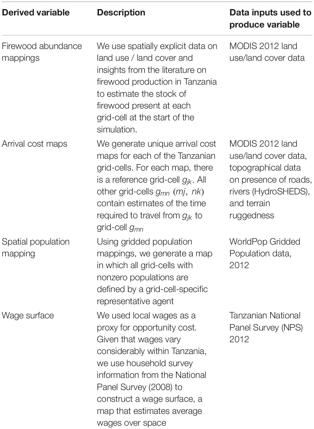
Table 1. Summary of key variables and data sources.

The key data inputs to our model the—firewood abundance mappings and arrival cost maps—are measured at a 500 m resolution. This may seem coarse when we’re modeling human movement on foot: perhaps we will miss some interesting intra-cell dynamics. But our choice to use this spatial resolution was motivated by the following factors. First, our model is intended to be policy relevant, such that it can be executed for any country or even on a global scale, as is the case with many other ecosystem service models (Johnson et al., 2021). But many countries do not have land cover data at high spatial resolution. By using coarser and globally available land cover data, we can enhance the generalizability of our approach. Moreover, our model still implicitly captures intra-cell competition since the remaining stock of agent i depends on the foraging activities of other agents over the cells in agent i′s zero profit zone.

An additional concern is that, at such a coarse resolution, agents will often forage at the grid cell they start at and will rarely travel. But again, agent competition will often prevent this from occurring. Agents with earlier iteration steps will often deplete the grid-cell that agent i starts out on, forcing agent i to leave their grid-cell in order to harvest. Moreover, the simulation only reaches equilibrium when agents have exhausted all net-positive profits. As stocks are depleted, the agent will have to go further from their starting point until all possible profits have been collected.

2.2.1 Case Study Area

We apply the simulation to a case study on firewood collection in Tanzania. Firewood is the predominant energy source for many Tanzanians. Faße and Grote (2013) find that 97.5% of Tanzanian households use firewood for heating and cooking. Luoga et al. (2002) argue that firewood provides 88% of all energy consumption in Tanzania. Firewood consumption is especially high for households further from urban areas (Luoga et al., 2002). For low-income African countries such as Tanzania, per person daily firewood consumption estimates range from 1.0 to 1.8 kg (Bério, 1984; Biran et al., 2004; Faße and Grote, 2013), though economies of scale with respect to the number of household members do exist (Biran et al., 2004).

Past literature suggests that Tanzanian households collect firewood for their own consumption, with very little firewood bought and sold in markets (Faße and Grote, 2013). Consumption of firewood may not require pecuniary costs for the household, but the time costs can be substantial. Average time requirements generally range from 10 min to over an hour per day on firewood collection, which is often undertaken by women and children (Biran et al., 2004; Levison et al., 2018). Although firewood foraging may impose time costs on the households, there are many scenarios in which household collection for consumption is an optimal strategy that maximizes the household’s welfare returns to its time allocations.

The model is designed to provide estimates of ecosystem service value under short-run conditions. It does not incorporate charcoal production and consumption, given the low usage of this energy source in Tanzania (Luoga et al., 2002). Relative to firewood, charcoal is considered more threatening to forest cover given that its production requires the burning of forested areas and is often done at larger scales (Hosier, 1993; van der Plas, 1995). But even if firewood consumption does not negatively impact the tree canopy, household extraction may still prove unsustainable if the forest cannot regenerate dead wood quickly enough to keep up with household demand (Luoga et al., 2000).

2.2.2 Firewood Abundance Mappings

Our simulation requires an initial mapping of firewood available in all grid-cells at the first iteration step. To produce this yield mapping over Tanzania, we use the Moderate-resolution Imaging Spectroradiometer (MODIS) Land Cover Type dataset for 2012. From the MODIS data product, we specifically choose the data derived from the global vegetation classification scheme (Friedl et al., 2010). Figure 4 shows the MODIS data for all of Tanzania (Panel A) as well as a subset near Mount Kilimanjaro (Panel B).

FIGURE 4

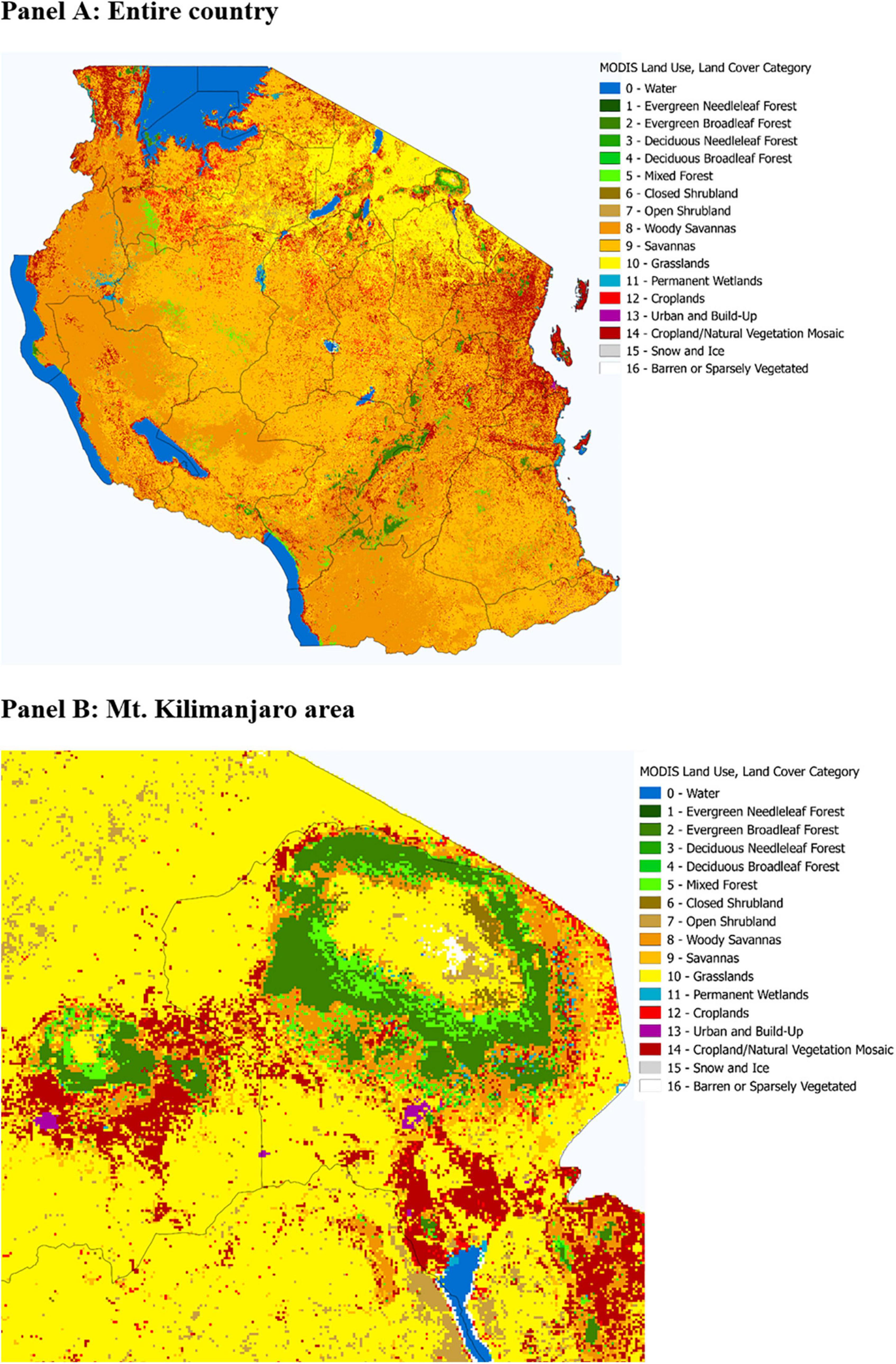
Figure 4. MODIS LULC data processed for Tanzania.

We calculate the supply of firewood in each grid-cell by combining MODIS LULC data with literature values on firewood per hectare on different land types (see Supplementary Section 2 for a discussion of the literature values used for estimated cubed meters of firewood by LULC classification).

2.2.3 Mapping Agent Locations

We use WorldPop 2012 gridded data to identify the distribution of the Tanzanian population over space. WorldPop uses country census data and remotely sensed imagery on settlement characteristics to estimate annual population counts at the grid-cell level (Gaughan et al., 2013).

We re-classify the 2012 gridded population maps such that each grid-cell with population greater than zero is defined as having one representative agent. This representative agent makes production choices at its respective iteration step, but its demand reflects the size of the entire population on the representative agent’s grid-cell. Hence, if there are x_mnresidents on grid-cell g_mn, the representative agent’s firewood demands are equivalent to the collective demand of all x_mnresidents. This approach enhances computational efficiency (by reducing the number of agents) while ensuring that demand still reflects the grid-cell’s population size.

2.2.4 Calculating a Wage Surface

We obtain wage data using the Tanzanian National Panel Survey (NPS) 2012 wave, which includes approximately 16,000 individuals in nearly 4,000 households. Every household in the NPS has a recorded latitude and longitude location, allowing for spatially explicit matching of ecosystem data and economic data. To ensure respondent confidentiality, respondent geocoordinates are randomly displaced by 3–10 km within the respondent’s enumeration area. Because the displacement is random, it will reduce the precision of our wage mapping but will not induce bias. Unfortunately, this random displacement also prevents robust validation (see Supplementary Sections 1, 5).

We use the NPS data to calculate a wage surface for Tanzania that reflects the opportunity costs of foraging forest products. Because firewood can often be collected from common property areas, the main input cost is determined by what income the agent could have generated with their time. Because the surveys only reflect wages for 409 enumeration areas in the country, we developed a method for creating a wage surface from these sparse points that predicts the wages in areas unobserved in the NPS. This method relied on an inverse distance weighted interpolation algorithm to create a continuous surface based on the household survey data (see Zimmerman et al., 1999 or Mueller et al., 2004 for a discussion of different interpolation techniques relevant to this type of problem). This approach relies on the assumption that the wages in grid-cells unobserved by the NPS are systematically related to their (inversely weighted) distance from observed cells. While we cannot test the validity of the assumption in this paper, we feel that our estimated wage surface serves as an improvement over approaches that assume no geographic component to wages. This process yields a grid-cell mapping of predicted average wages across all of Tanzania (shown in Supplementary Figure 1).

2.2.5 Travel and Arrival Cost Networks

Our final data input required for implementing our simulation is a set of arrival cost maps derived based on traversal cost mappings. Traversal cost denotes the amount of time it takes an agent to traverse from one side of one grid-cell to the other when traveling on one of the cardinal axes. Arrival costs refer to the time required for an agent starting at a reference grid-cell to arrive to other grid-cells in the area. We explain the method of deriving arrival cost and traversal cost mappings below and go into farther detail in Supplementary Section 3.

To construct the traversal cost maps, we assume that humans walk at 1.38 m per second on paved surfaces, based on the median value reported in a 31-country study by Levine and Norenzayan (1999). We account for slower travel over different land types based on differences in traversal times relative to paved surfaces for each land cover classification (see Supplementary Section 3 for travel time per LULC type).

Applying the estimated travel times to the MODIS LULC data, we mapped the minutes necessary to traverse across a given grid-cell based on the LULC information alone. We then transform each grid-cell’s travel time based on the grid-cell’s intersection with relevant features, such as roads, rivers, and slope steepness. The final product is a traversal cost map that provides a comprehensive estimate of the time needed to cross the grid-cell, assuming all travel occurs on foot. The underlying assumption—of travel only occurring on foot—will likely not bias our results because walking remains the dominant mode of transport when foraging in forests and other rough terrain.

We use the traversal cost function and a route-finding algorithm to determine the time required to travel from one grid-cell to all surrounding grid-cells (not just adjacent cells). Route-finding is a common computational challenge for which there is no perfect solution. For example, using the most sophisticated route-finding algorithm is not computationally feasible across Tanzania at this resolution, so we developed our own path-finding algorithm that optimally combines four route-finding algorithms with varying degrees of precision (presented in Supplementary Section 3). The composite algorithm matches grid-cell pairs with the most efficient route-finding algorithm of the possible four, given the grid-cell’s position on the landscape. For each grid-cell, the optimal route-finding algorithm is the one that greatly increases accuracy while greatly reducing computational intensity.²

Using the composite algorithm, we define a set of arrival cost mappings. Each map demonstrates the cumulative traversal cost incurred when traveling from a reference grid-cell g_mn to other grid-cells g_jk based on the optimal travel route. Each arrival cost map is constructed such that it includes all grid-cells g_jk where a representative agent starting at g_mn can obtain zero or positive profit from foraging at g_jk given the initial state of the landscape.

Figure 5 shows an example of calculating traversal and arrival cost. The left image shows the traversal cost mapping, which uses topographical information to estimate the amount of time required to traverse a given grid-cell. The red paths where traversal costs are highest correspond with rivers, and the blue lines where traversal costs are lowest correspond with roads. The image on the right image shows the arrival costs based on a reference grid-cell at the center of the map. This tells us the amount of time required to walk from the center of the map to all other grid-cells based on the traversal cost map and our route-finding algorithm.

FIGURE 5

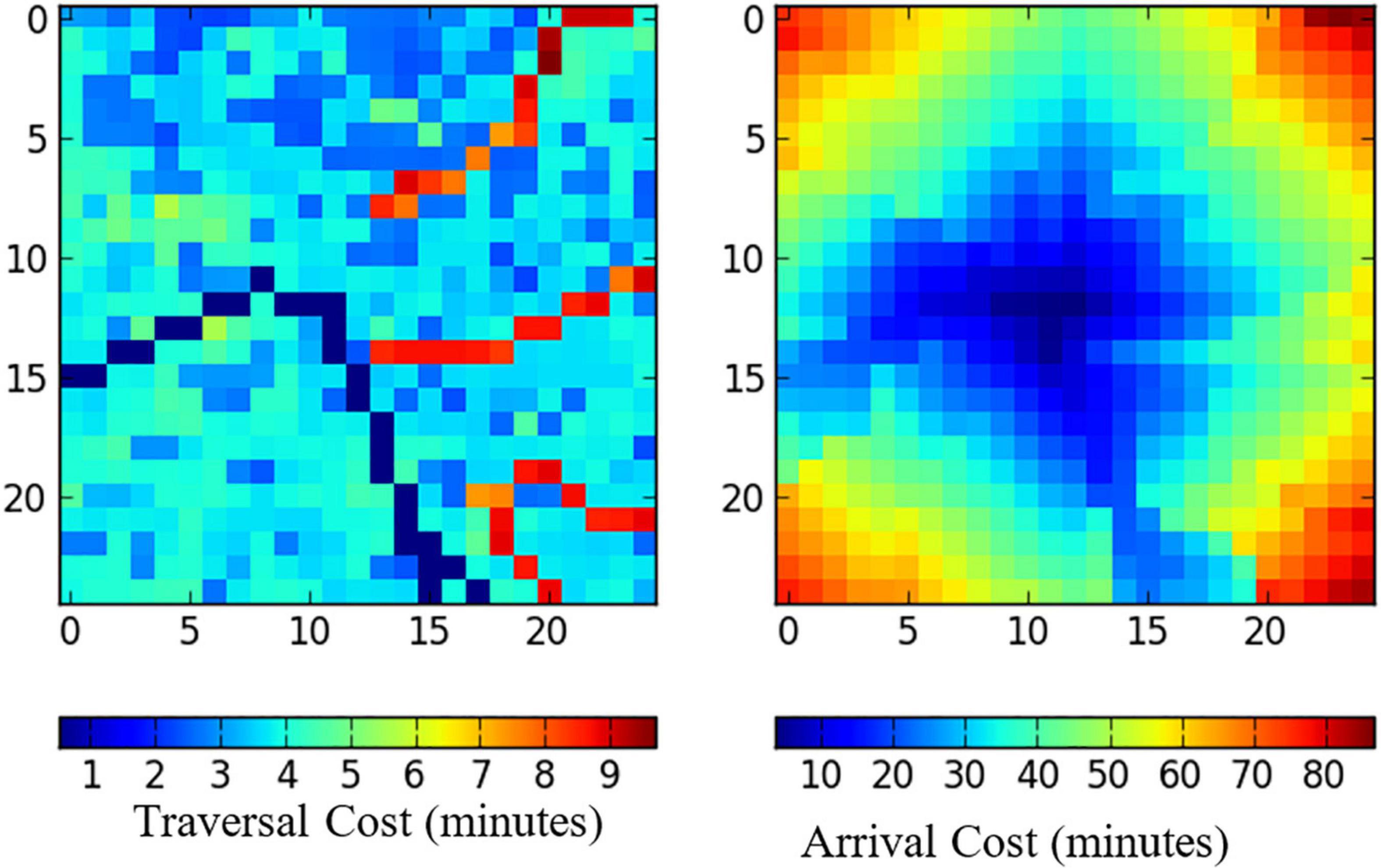
Figure 5. Traversal cost and arrival cost maps over an M by N matrix of grid-cells.

2.2.6 Agent Labor Endowments

The labor endowment of each agent is taken to be exogenous in this model. Each agent in this model represents the full population of the 500- by 500-m grid-cell. We define the labor endowment of an agent as the population of the grid-cell multiplied by the labor participation rate. Future work can easily extend this analysis to match location-specific labor participation rates, but this was not available for Tanzania. Figure 8 presents the total labor endowment available at the beginning of the simulation.

2.3 Sensitivity Analysis

As detailed in SI2, our firewood abundance maps are sensitive to assumptions we make about the stock of firewood over different land cover types in Tanzania. We further evaluate the sensitivity of our results to these assumptions by estimating our model under a different set of assumptions. We define eight alternative approaches to estimating the initial firewood stock based on land cover type. To determine these “scenarios,” we identify the assumptions in our model with the greatest uncertainty, given the range of estimates in the literature. We then modify our firewood stock predictions to see how these assumptions change when we believe that the firewood stock on a given grid-cell is higher or lower than in our main model. For example, given the broad range of estimates of the stock of firewood in Tanzanian forests, we re-run our simulation with a firewood abundance map that assigns forest grid-cells the same firewood stock as shrub grid-cells. We provide a full account of the different firewood abundance map production schemes in the Supplementary section (Supplementary Table 2 and Section 5).

Our model is also sensitive to the accuracy of our wage surface. The random spatial displacement of the village locations from which we derive the wage estimates for our wage surface is a source of measurement error. Consequently, we evaluate the results of our simulation when we set the wage lower (or higher) by reducing (or increasing) the average wage by the average within-village standard deviation of wages in the 2012 NPS data, which is 13.1%.

3 Results

We present results that show where and how agents gather and gain utility from firewood based on our agent-based simulation. In our sensitivity analysis, we also evaluate how the resulting equilibrium shifts as our assumptions about the landscape or the agents change.

3.1 Calculating Supply

We calculate the supply of firewood by combing LULC data with literature values on firewood per hectare on different land types. As discussed in the data section, the LULC data comes from MODIS, a land sensing and classification project by NASA. MODIS identifies 16 land use categories, of which five are forest, two are shrublands and two are savannah. We apply the literature values discussed in Supplementary Section 2 and present the per grid-cell abundance values for firewood in each of these 16 land categories. In Supplementary Section 5, we report the aggregate firewood supply in both the baseline scenarios and the alternative scenarios used for our sensitivity analysis. Because the results of this model are sensitive to how we parameterize firewood abundance, the alternative scenarios show us how results change when we make different assumptions about how much firewood is available for each land type.

Figure 6 shows the supply of firewood available before the first iteration of gathering. Most land is in shrublands and savannah, though there exist areas of dense forest around Mount Kilimanjaro and in the natural reserve land in the southeast and northwest. The values presented for abundance are biophysical observations only. The agent considers the firewood stock on a grid-cell, taking into account the value of fuel, their local wage, and the travel related collection costs.

FIGURE 6

Figure 6. Firewood supply (m³ firewood per grid-cell).

After the simulation has run, forests near agents who find it profitable to forage will be depleted. This is shown in Figure 7, which plots the cubic meters of firewood supply taken from each grid-cell. The areas shown as foraged are determined by where demand is the greatest, where supply is the greatest, and where costs make collection relatively more valuable than the fuel substitute. We find high degrees of foraging on the southern slopes of Mount Kilimanjaro, in the shrublands to the south of Lake Victoria, and along the arterial transportation corridors connected to Dar es Salaam. These results suggest that increasing supply leads to more foraging when the supply is within an agent’s zero profit zone, meaning it is nearby. Higher accessibility in supply leads to more foraging.

FIGURE 7

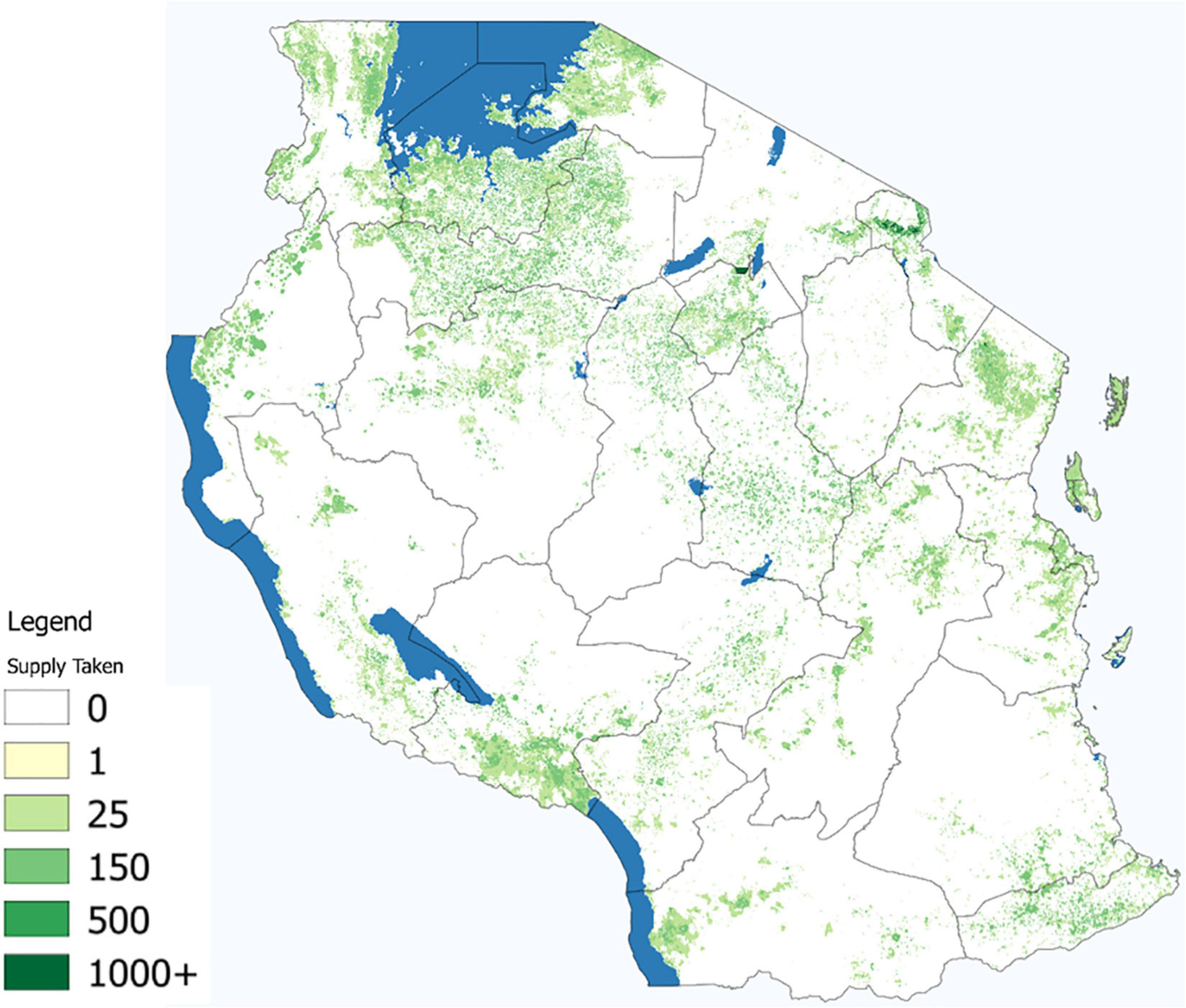
Figure 7. Supply extracted (m³ firewood per grid-cell).

FIGURE 8

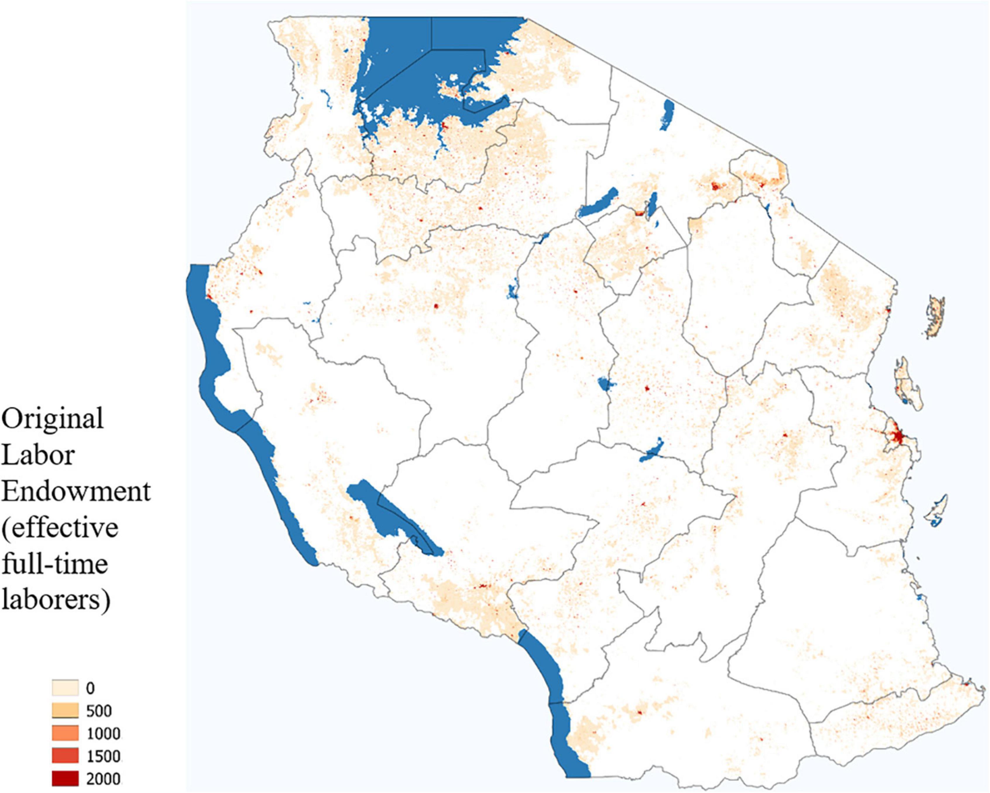
Figure 8. Initial labor endowment.

3.2 Calculating Consumption and Demand

For every cubic meter of firewood gathered, there is a corresponding amount of firewood that arrives at an agent’s household location and is consumed. We can characterize the benefits of this firewood consumption in multiple ways: based on the value of firewood that accrues to each agent after travel costs are accounted for; based on the amount of labor spent by each agent on foraging; or based on the raw amount of firewood that arrives at the agent’s household. The last measure, while very easy to define, is very difficult to interpret because demand is determined endogenously by the agent’s household utility maximization decisions. As we point out while introducing our model, firewood and leisure are not substitutes in consumption, and households experience diminishing marginal utility as they consume increasing amounts of one good at the expense of the other. A household that consumes a lot of firewood may in fact be worse off than a household that consumes slightly less firewood, since the marginal returns to the household for consuming the last units of firewood are low and come at the expense of leisure time, another good the agent values. Thus, care must be taken when evaluating consumption of firewood with respect to agent welfare.

The initial distribution of labor (Figure 8) is assumed to be exogenous, but it endogenously determines labor allocation choices. Figure 9 presents the amount of labor on each grid-cell that was used to purchase the fuel substitute (usually kerosene). A clear result of this model is that locations with high population density purchase the majority of the fuel substitute. This is because the agents on the edges of the urban centers deplete all nearby firewood and thus everyone on the interior of the dense population area has no profitable firewood available to forage.

FIGURE 9

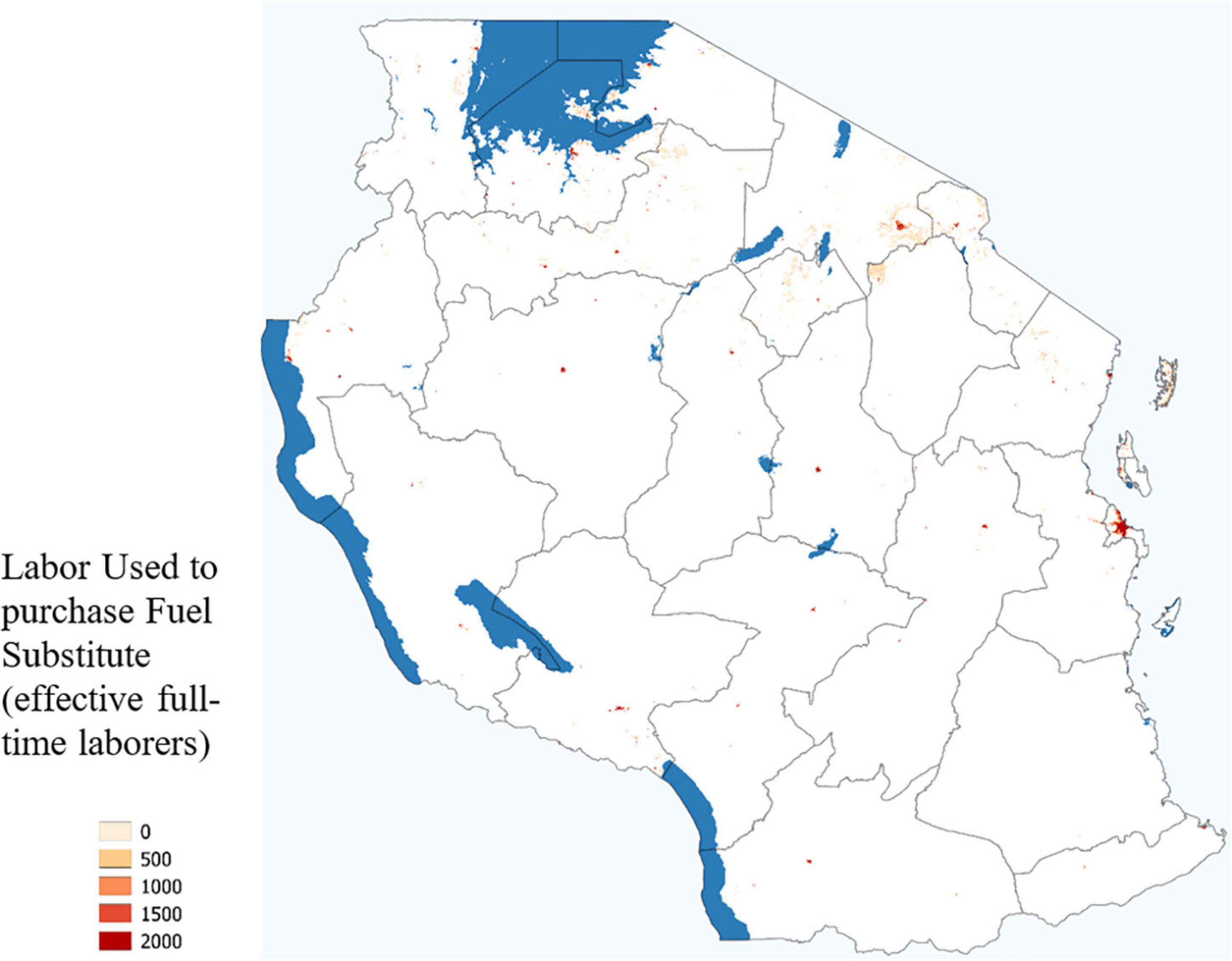
Figure 9. Labor used to purchase fuel substitute.

The majority of labor used to satisfy fuel demand was dedicated to collecting firewood, as shown in Figure 10. The values shown in this figure reflect agents choosing optimal travel routes and making the utility maximizing choice among foraging, laboring and leisure.

FIGURE 10

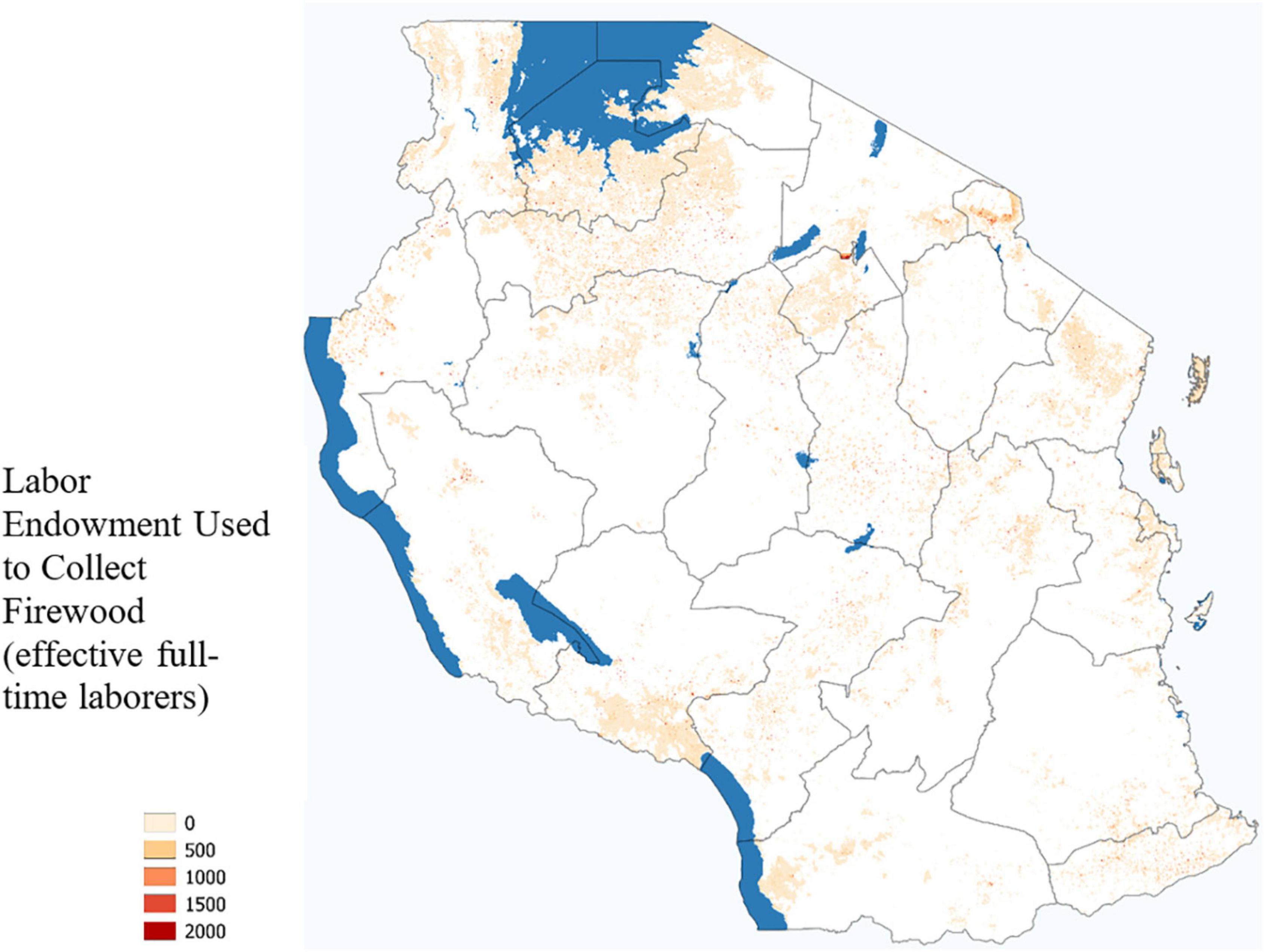
Figure 10. Labor used to collect firewood.

Accounting for labor usage and supply of firewood taken, we can now calculate the profit (or if desired, utility) that each agent generates. Figure 11 plots the value in 2008 TSH that each agent collects from foraging at a national scale (top) and zoomed in to the area around Mt. Kilimanjaro.

FIGURE 11

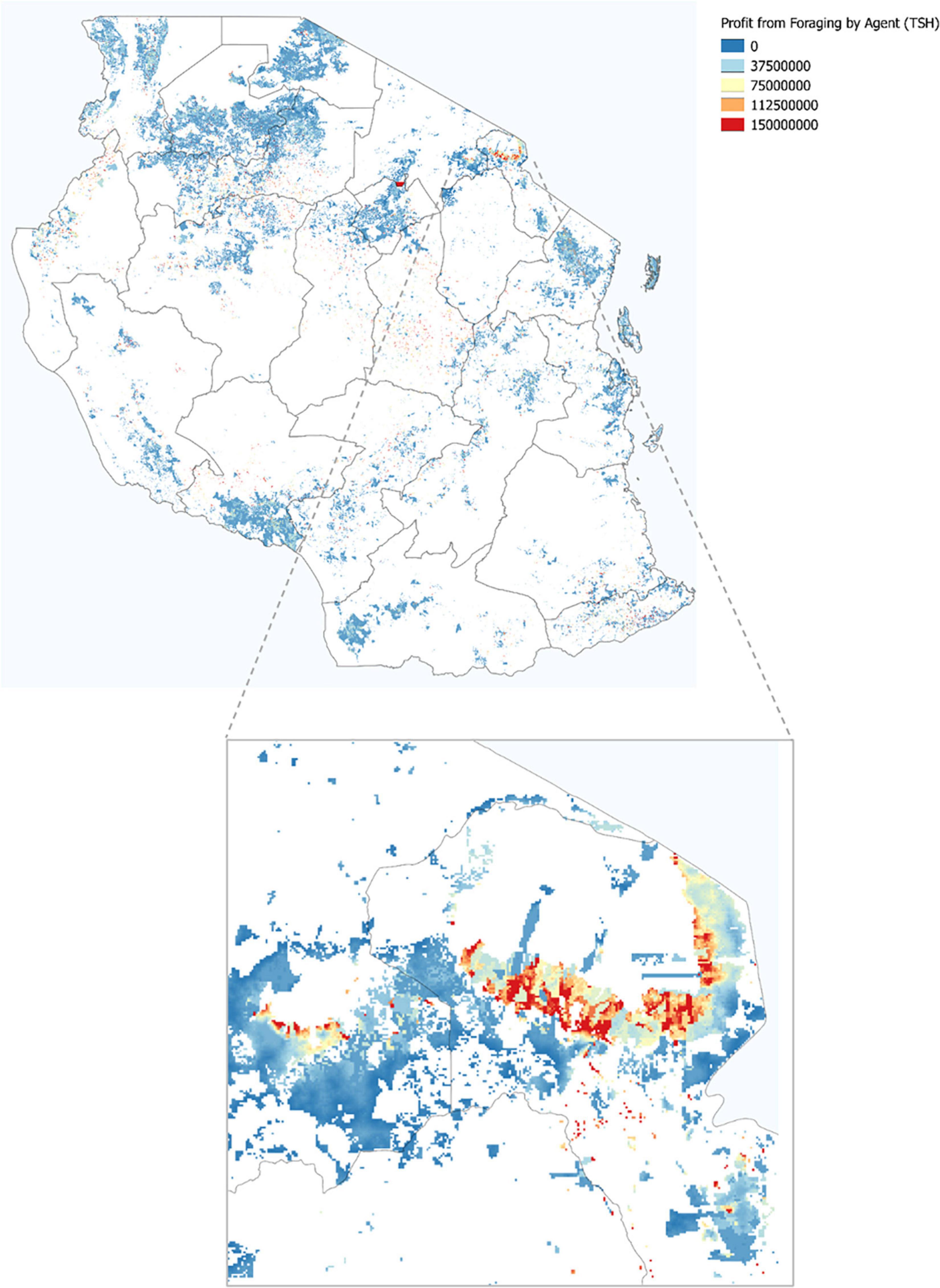
Figure 11. Profit earned by each agent.

Figure 11 highlights the complexity of behavior that arises in response to competition. In the western area of the Mt. Kilimanjaro subplot, we observe agents at the outskirts of a high quality forest who obtain a high, positive profit from foraging, with a decreasing gradient of profit obtained as we move southwest away from the forest boundary. The decrease arises because the agents farther to the south must travel ever farther to get the firewood. Note that the agents plotted with yellow or blue (lower profits) may well gather the same (or more) firewood than the agents right on the border of the forest due to tradeoffs implied by their household optimization decisions.

Next, we compare our predictions of aggregate firewood collected to values derived from past literature on firewood stock in Tanzania. Values from existing studies suggest that annual firewood demand is between 25.8 and 55.5 million m³. Our primary model predicts 66.7 million m³ of firewood will be gathered. This is above, but within the order of magnitude reported in the literature. The overestimated value here is very likely a result of wrong assumptions on mean harvestable volume per hectare. The range of values identified from the literature (14–117 m³ha⁻¹year⁻¹) is based on a relatively small sample of land which was primarily covered in woodlands. Newer estimates suggest the value should be closer to the minimum value of this distribution than to the mean value, which we used. And since the majority of Tanzania is shrublands and savannah, which may have lower densities of firewood, it is not surprising that using the woodlands estimates would result in overstating the national effect.

3.3 Sensitivity Analysis

In the SI, we report the demand met and the profit earned for each scenario, along with a comparison of change in profit compared to the baseline scenario, detailed in SI Table S.5.2. This table shows that several of the scenarios with lower firewood density yield aggregate firewood collection outcomes that are closer to literature values. For instance, a scenario with reduced firewood concentrations on forests and shrublands scenario predicts approximately 41.4 million m³, which is comfortably within the range of estimated consumption. See Supplementary Figures 5.1 for a plotted comparison of these scenarios and their deviation from the baseline assumptions.

4 Discussion and Conclusion

We apply agent-based simulation to firewood collection in Tanzania. By doing so, we account for geospatial heterogeneity and inter-agent competition for foraging goods to evaluate where NTFP extraction occurs and the resulting profits for households. Practitioners of ecosystem service valuation are eager to include NTFP in their valuation exercises, but challenges in conveying spatial heterogeneity and non-cooperative behavior have prevented widespread application of non-timber forest product valuation to conservation planning. Our agent-based simulation aims to break through the barrier that has prevented the valuation of non-timber products in forests, and thus, provide a method for more accurately understanding values of forests that are very often missed.

Our study provides key insights into the value of NTFP. Households in countries such as Tanzania often harvest NTFP for private consumption, so we cannot rely on a market price as an indicator of the benefit that society obtains from these products. Without a market price, estimates of the value of intact natural lands that generate NTFP will under-estimate the benefits of conservation. Our model yields pecuniary estimates of the value of a year’s worth of firewood in Tanzania: 14,800 billion 2008 Tanzanian Schillings (TSH), about 12 million 2008 USD. This high aggregate value highlights the importance of thinking carefully about land use policy: conservation can help ensure that poor households can access firewood and maximize their welfare, but conservation policies that prevent human entry onto landscapes with firewood stocks may also hurt those who derive high benefits from firewood harvesting. Our model also provides insights into where people harvest firewood most, which can help policymakers determine optimal place-specific policies with respect to conservation and human activity.

The primary limitation of our model is that we cannot fully validate it. We compare aggregate firewood harvests in our model to estimates from the literature: these are within the same order of magnitude. But such aggregations can be misleading and belie large biases only discernable at higher resolutions (Levin, 1992; May et al., 2015). As data limitations currently prevent further validation, we urge our readers to consider our current study as a “proof of concept.”

The emphasis of this model (and of most ABS) is not to predict specific actions, but to describe overall outcomes of the system and understand what affects these outcomes, a framework known as pattern-oriented modeling (Grimm et al., 2005). Although our model’s predictions appear valid on an aggregate level (relative to other national estimates), it remains difficult to validate at the grid-cell level due to the random displacement of village geolocations in the NPS. If these data were not obscured, it would be straightforward to compare model predictions on how many hours each agent will forage for firewood, and then compare these predictions to household survey data on firewood collection. Specifically, household survey data that report hours spent foraging could be compared against the foraging and travel time predicted by the model, which is shown in Figure 12 for agents near Mount Kilimanjaro. Note that there is extreme variation at small scales. This is an expected outcome of the model given that firewood is not transported very far and that it has high transportation costs, but it also highlights the difficulty of making specific predictions on agent actions.

FIGURE 12

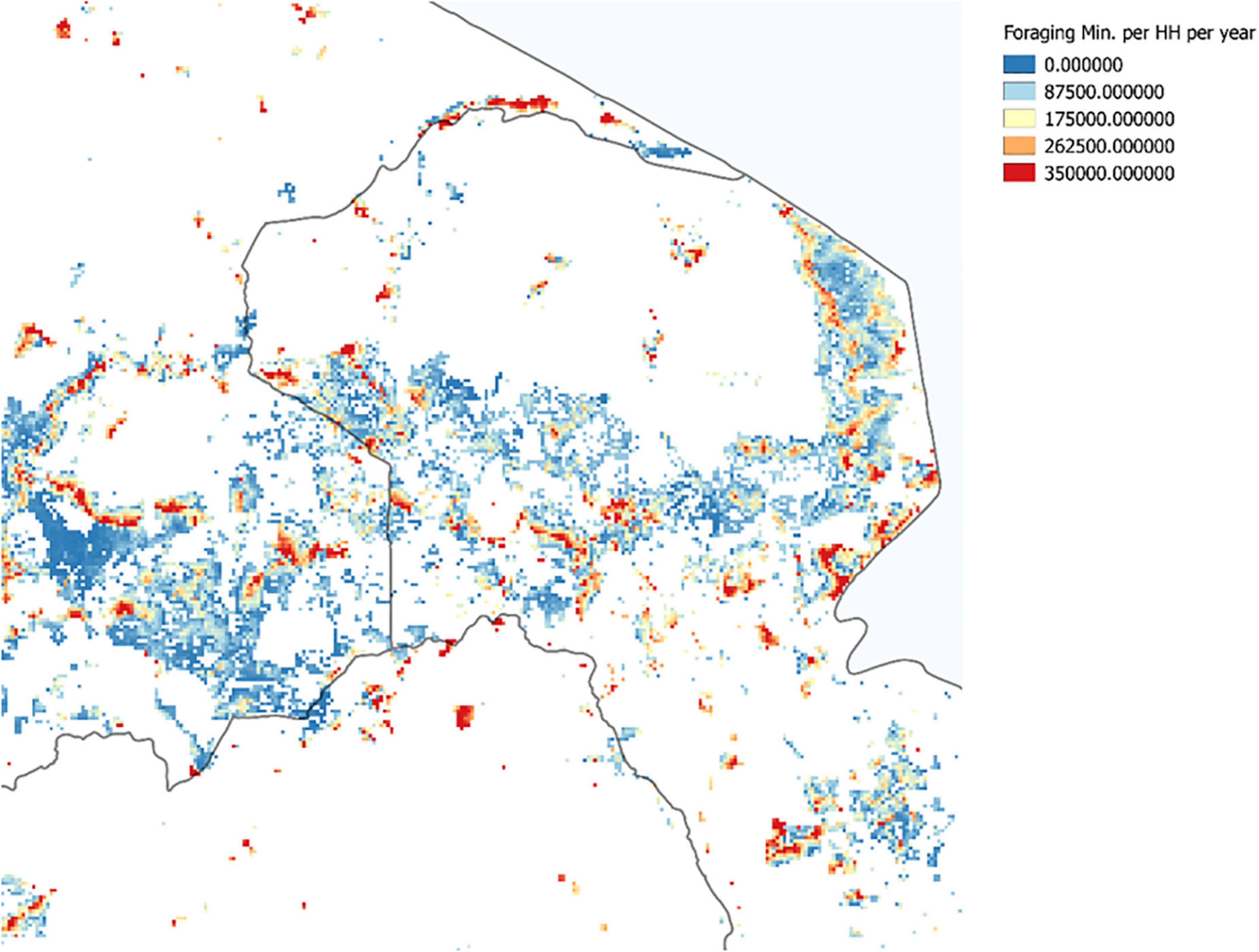
Figure 12. Travel time spent in minutes per household per year (near Mt. Kilimanjaro).

Future research can use our modeling and simulation approach, along with locally representative data, to estimate NTFP extraction for particular contexts. The model would indeed benefit from additional calibration using more extensive household and bioclimatic data. Researchers can also use our model to examine how NTFP foraging and household outcomes change under different land use policy scenarios. Such analyses would highlight positive or negative spillovers from policies that influence household access to NTFP, such as rezoning common pool forests as protected areas.

Data Availability Statement

The datasets presented in this study can be found in online repositories. The names of the repository/repositories and accession number(s) can be found in the article/Supplementary Material.

Author Contributions

JJ conceived the study, designed the simulation, gathered/generated the input data, and estimated the main results. CS contributed to the idea clarification. Both authors contributed to the analysis of the results, drafting and revision of the manuscript, and approved the submitted version.

Funding

This research was supported by a Graduate Research Fellowship from the University of Minnesota and from start-up research funds from the Department of Applied Economics at the University of Minnesota.

Conflict of Interest

The authors declare that the research was conducted in the absence of any commercial or financial relationships that could be construed as a potential conflict of interest.

Publisher’s Note

All claims expressed in this article are solely those of the authors and do not necessarily represent those of their affiliated organizations, or those of the publisher, the editors and the reviewers. Any product that may be evaluated in this article, or claim that may be made by its manufacturer, is not guaranteed or endorsed by the publisher.

Supplementary Material

The Supplementary Material for this article can be found online at: https://www.frontiersin.org/articles/10.3389/fevo.2022.845435/full#supplementary-material

Footnotes

1. ^ Other studies have applied a spatial natural capital lens to studies of resources that are not stationary, such as fish populations. See for example Costello et al. (2019).
2. ^ This approach is able to provide a large computation speed increase because many route finding problems are quite simple (for instance, traversing a uniformly flat field) and the simpler algorithms identify the optimal route in a faction of the computational time necessary for more complex route-finding algorithms.

References

Albers, H. J., and Robinson, E. J. Z. (2013). A review of the spatial economics of non-timber forest product extraction: implications for policy. Ecol. Econ. 92, 87–95. doi: 10.1016/j.ecolecon.2012.01.021

CrossRef Full Text | Google Scholar

Bardhan, P., and Udry, C. (1999). Development Microeconomics. Oxford: Oxford University Press.

Google Scholar

Barthélemy, M. (2011). Spatial networks. Phys. Rep. 499, 1–101. doi: 10.1016/j.physrep.2010.11.002

CrossRef Full Text | Google Scholar

Bério, A.-J. (1984). Household food distribution: the analysis of time allocation and activity patterns in nutrition and rural development planning. Food Nutr. Bull. 6, 1–16. doi: 10.1177/156482658400600113

CrossRef Full Text | Google Scholar

Biran, A., Abbot, J., and Mace, R. (2004). Families and firewood: a comparative analysis of the costs and benefits of children in firewood collection and use in two rural communities in Sub-Saharan Africa. Hum. Ecol. 32, 1–25. doi: 10.1023/B:HUEC.0000015210.89170.4e

CrossRef Full Text | Google Scholar

Black, A. J., and McKane, A. J. (2012). Stochastic formulation of ecological models and their applications. Trends Ecol. Evol. 27, 337–345. doi: 10.1016/j.tree.2012.01.014

PubMed Abstract | CrossRef Full Text | Google Scholar

Blackwell, P. G. (1997). Random diffusion models for animal movement. Ecol. Model. 100, 87–102. doi: 10.1016/S0304-3800(97)00153-1

CrossRef Full Text | Google Scholar

Bošković, B., Chakravorty, U., Pelli, M., and Risch, A. (2018). The Effect of Forest Access on the Market for Fuelwood in India. FEEM Working Paper No. 21.2018. Available online at: https://ssrn.com/abstract=3209163 (accessed December 1, 2021).

Google Scholar

Cao, Y., Gillespie, D. T., and Petzold, L. R. (2006). Efficient step size selection for the tau-leaping simulation method. J. Chem. Phys. 124:044109. doi: 10.1063/1.2159468

CrossRef Full Text | Google Scholar

Chael, N., Crombez, C., and Vangerven, P. (2019). Spatial models, legislative gridlock, and resource policy reform. Annu. Rev. Resour. Econ. 11, 83–100. doi: 10.1146/annurev-resource-100517-022958

CrossRef Full Text | Google Scholar

Costanza, R., de Groot, R., Sutton, P., van der Ploeg, S., Anderson, S. J., Kubiszewski, I., et al. (2014). Changes in the global value of ecosystem services. Glob. Environ. Change 26, 152–158. doi: 10.1016/j.gloenvcha.2014.04.002

CrossRef Full Text | Google Scholar

Costello, C., Nkuiya, B., and Quérou, N. (2019). Spatial renewable resource extraction under possible regime shift. Am. J. Agric. Econ. 101, 507–527. doi: 10.1093/ajae/aay076

CrossRef Full Text | Google Scholar

Dou, Y., Deadman, P., Berbés-Blázquez, M., Vogt, N., and Almeida, O. (2020). Pathways out of poverty through the lens of development resilience: an agent-based simulation. Ecol. Soc. 25:3. doi: 10.5751/ES-11842-250403

PubMed Abstract | CrossRef Full Text | Google Scholar

Epstein, J. M., and Axtell, R. L. (1996). Growing Artificial Societies: Social Science from the Bottom Up. Cambridge, MA: The MIT Press. doi: 10.7551/mitpress/3374.001.0001

CrossRef Full Text | Google Scholar

Faße, A., and Grote, U. (2013). The economic relevance of sustainable agroforestry practices—An empirical analysis from Tanzania. Ecol. Econ. 94, 86–96. doi: 10.1016/j.ecolecon.2013.07.008

CrossRef Full Text | Google Scholar

Friedl, M. A., Sulla-Menashe, D., Tan, B., Schneider, A., Ramankutty, N., Sibley, A., et al. (2010). MODIS collection 5 global land cover: algorithm refinements and characterization of new datasets. Remote Sens. Environ. 114, 168–182.

Google Scholar

Gaughan, A. E., Stevens, F. R., Linard, C., Jia, P., and Tatem, A. J. (2013). High resolution population distribution maps for Southeast Asia in 2010 and 2015. PLoS One 8:e55882. doi: 10.1371/journal.pone.0055882

PubMed Abstract | CrossRef Full Text | Google Scholar

Gillespie, D. T. (1977). Exact stochastic simulation of coupled chemical reactions. J. Phys. Chem. 81, 2340–2361. doi: 10.1021/j100540a008

CrossRef Full Text | Google Scholar

Glenk, K., Johnston, R. J., Meyerhoff, J., and Sagebiel, J. (2020). Spatial dimensions of stated preference valuation in environmental and resource economics: methods, trends and challenges. Environ. Resour. Econ. 75, 215–242. doi: 10.1007/s10640-018-00311-w

CrossRef Full Text | Google Scholar

Graubner, M., Salhofer, K., and Tribl, C. (2021). A line in space: pricing, location, and market power in agricultural product markets. Annu. Rev. Resour. Econ. 13, 85–107. doi: 10.1146/annurev-resource-110220-010922

CrossRef Full Text | Google Scholar

Grimm, V., Railsback, S. F., Vincenot, C. E., Berger, U., Gallagher, C., DeAngelis, D. L., et al. (2020). The ODD protocol for describing agent-based and other simulation models: a second update to improve clarity, replication, and structural realism. J. Artif. Soc. Soc. Simul. 23:7.

Google Scholar

Grimm, V., Revilla, E., Berger, U., Jeltsch, F., Mooij, W. M., Railsback, S. F., et al. (2005). Pattern-oriented modeling of agent-based complex systems: lessons from ecology. Science 310, 987–991. doi: 10.1126/science.1116681

PubMed Abstract | CrossRef Full Text | Google Scholar

Hare, M., and Deadman, P. (2004). Further towards a taxonomy of agent-based simulation models in environmental management. Math. Comput. Simul. 64, 25–40. doi: 10.1016/S0378-4754(03)00118-6

CrossRef Full Text | Google Scholar

Hosier, R. H. (1993). Charcoal production and environmental degradation. Energy Policy 21, 491–509. doi: 10.1016/0301-4215(93)90037-G

CrossRef Full Text | Google Scholar

Hotelling, H. (1929). Stability in competition. Econ. J. 39, 41–57.

Google Scholar

Huber, R., Bakker, M., Balmann, A., Berger, T., Bithell, M., Brown, C., et al. (2018). Representation of decision-making in European agricultural agent-based models. Agric. Syst. 167, 143–160. doi: 10.1016/j.agsy.2018.09.007

CrossRef Full Text | Google Scholar

Johnson, J. A., Ruta, G., Baldos, U., Cervigni, R., Chonabayashi, S., Corong, E., et al. (2021). The Economic Case for Nature: A Global Earth-Economy Model to Assess Development Policy Pathways. Washington, DC: World Bank.

Google Scholar

Kool, J. T., Moilanen, A., and Treml, E. A. (2013). Population connectivity: recent advances and new perspectives. Landsc. Ecol. 28, 165–185. doi: 10.1007/s10980-012-9819-z

CrossRef Full Text | Google Scholar

Kranstauber, B., Kays, R., LaPoint, S. D., Wikelski, M., and Safi, K. (2012). A dynamic Brownian bridge movement model to estimate utilization distributions for heterogeneous animal movement. J. Anim. Ecol. 81, 738–746. doi: 10.1111/j.1365-2656.2012.01955.x

PubMed Abstract | CrossRef Full Text | Google Scholar

Le, Q. B., Seidl, R., and Scholz, R. W. (2012). Feedback loops and types of adaptation in the modelling of land-use decisions in an agent-based simulation. Environ. Model. Softw. 2, 83–96. doi: 10.1016/j.envsoft.2011.09.002

CrossRef Full Text | Google Scholar

Lehman, C., Keen, A., and Barnes, R. (2012). “Trading Space for Time: Constant-Speed Algorithms for Managing Future Events in Scientific Simulations,” in Proceedings of the International Conference on Scientific Computing (CSC), Las Vegas, NV.

Google Scholar

Levin, S. A. (1992). The problem of pattern and scale in ecology: the Robert H. MacArthur Award Lecture. Ecology 73, 1943–1967. doi: 10.2307/1941447

CrossRef Full Text | Google Scholar

Levine, R. V., and Norenzayan, A. (1999). The pace of life in 31 countries. J. Cross Cult. Psychol. 30, 178–205.

Google Scholar

Levison, D., DeGraff, D. S., and Dungumaro, E. W. (2018). Implications of environmental chores for schooling: children’s time fetching water and firewood in Tanzania. Eur J. Dev. Res. 30, 217–234. doi: 10.1057/s41287-017-0079-2

PubMed Abstract | CrossRef Full Text | Google Scholar

Luoga, E. J., Witkowski, E. T. F., and Balkwill, K. (2000). Economics of charcoal production in miombo woodlands of eastern Tanzania: some hidden costs associated with commercialization of the resources. Ecol. Econ. 35, 243–257. doi: 10.1016/S0921-8009(00)00196-8

CrossRef Full Text | Google Scholar

Luoga, E. J., Witkowski, E. T. F., and Balkwill, K. (2002). Harvested and standing wood stocks in protected and communal miombo woodlands of eastern Tanzania. For. Ecol. Manage. 164, 15–30. doi: 10.1016/S0378-1127(01)00604-1

CrossRef Full Text | Google Scholar

May, F., Huth, A., and Wiegand, T. (2015). Moving beyond abundance distributions: neutral theory and spatial patterns in a tropical forest. Proc. Biol. Sci. 282:20141657. doi: 10.1098/rspb.2014.1657

PubMed Abstract | CrossRef Full Text | Google Scholar

Miteva, D. A., Kramer, R. A., Brown, Z. S., and Smith, M. D. (2017). Spatial patterns of market participation and resource extraction: fuelwood collection in Northern Uganda. Am. J. Agric. Econ. 99, 1008–1026. doi: 10.1093/ajae/aax027

CrossRef Full Text | Google Scholar

Mueller, T. G., Pusuluri, N. B., Mathias, K. K., Cornelius, P. L., Barnhisel, R. I., and Shearer, S. A. (2004). Map quality for ordinary kriging and inverse distance weighted interpolation. Soil Sci. Soc. Am. J. 68, 2042–2047.

Google Scholar

Oraby, T., Tyshenko, M. G., Maldonado, J. C., Vatcheva, K., Elsaadany, S., Alali, W. Q., et al. (2021). Modeling the effect of lockdown timing as a COVID-19 control measure in countries with differing social contacts. Sci. Rep. 11:3354. doi: 10.1038/s41598-021-82873-2

PubMed Abstract | CrossRef Full Text | Google Scholar

Patterson, T. A., Thomas, L., Wilcox, C., Ovaskainen, O., and Matthiopoulos, J. (2008). State–space models of individual animal movement. Trends Ecol. Evol. 23, 87–94. doi: 10.1016/j.tree.2007.10.009

PubMed Abstract | CrossRef Full Text | Google Scholar

Ramsey, F. (1928). A mathematical theory of saving. Econ. J. 38, 543–559.

Google Scholar

Rassweiler, A., Costello, C., and Siegel, D. A. (2012). Marine protected areas and the value of spatially optimized fishery management. Proc. Natl. Acad. Sci. U.S.A. 109, 11884–11889. doi: 10.1073/pnas.1116193109

PubMed Abstract | CrossRef Full Text | Google Scholar

Rodrigue, J.-P. (2020). The Geography of Transport Systems, 5th Edn. Milton Park: Routledge.

Google Scholar

Schreinemachers, P., and Berger, T. (2011). An agent-based simulation model of human–environment interactions in agricultural systems. Environ. Model. Softw. 26, 845–859. doi: 10.1016/j.envsoft.2011.02.004

CrossRef Full Text | Google Scholar

Singh, I., Squire, L., and Strauss, J. (1986). Agricultural Household Models: Extensions, Applications, and Policy. Washington, DC: The World Bank.

Google Scholar

Sterner, E. O., Robinson, E. J. Z., and Albers, H. J. (2018). Location choice for renewable resource extraction with multiple non-cooperative extractors: a spatial Nash equilibrium model and numerical implementation. Lett. Spat. Resour. Sci. 11, 315–331. doi: 10.1007/s12076-018-0215-4

CrossRef Full Text | Google Scholar

Turner, K. G., Anderson, S., Gonzales-Chang, M., Costanza, R., Courville, S., Dalgaard, T., et al. (2016). A review of methods, data, and models to assess changes in the value of ecosystem services from land degradation and restoration. Ecol. Model. 319, 190–207. doi: 10.1016/j.ecolmodel.2015.07.017

CrossRef Full Text | Google Scholar

van der Plas, R. (1995). Burning Charcoal Issues. Energy Issues. Washington, DC: World Bank.

Google Scholar

Wilkinson, D. J. (2019). Stochastic Modelling for Systems Biology, Third Edn. Milton Park: Routledge.

Google Scholar

Zimmerman, D., Pavlik, C., Ruggles, A., and Armstrong, M. P. (1999). An experimental comparison of ordinary and universal kriging and inverse distance weighting. Math. Geol. 31, 375–390.

Google Scholar