Apparent evolutionary maladaptation and inference from reciprocal transplants

1. Introduction

Evolutionary biologists and ecologists have based their work on the premise that the evolutionary response to environmental change in nature should be adaptive. That is, when populations face changing conditions that make them less adapted, they are expected to evolve in a way that strives to restore the fitness they have lost in the process. Yet, studies conducted in natural ecosystems as well as in the laboratory frequently fail to show evidence of local adaptation. A sizeable number of studies report the absence of adaptation, insufficient adaptation or even an evolutionary response that is worse, from a fitness perspective, than no change at all would have been. A meta-analysis of reciprocal transplant experiments estimated that the signature of local adaptation (where resident populations have higher fitness than foreign populations) occurred in 70% of cases (Hereford, 2009). This means that in 30% of cases populations were found to be maladapted to their environment, a result that might be an underestimate given that there is likely a reporting bias in favor of studies that “prove” adaptation. In the same vein, another meta-analysis focusing on selection coefficients found that in 64% of cases the mean trait value displayed by the studied populations was more than one phenotypic standard deviation away from the optimal trait value (Estes and Arnold, 2007). The perplexing ubiquity of populations in maladaptive states has led to two recent special issues on the topic of “maladaptation” in the journals American Naturalist and Evolutionary Applications. In addition to rallying papers with new case studies of maladaptation (Brady et al., 2019c; Fraser et al., 2019; Loria et al., 2019), the introductory articles of these special issues provide insightful analyses on the potential causes and mechanisms (Brady et al., 2019a,b).

In the present theoretical study we perform a closer investigation of a phenomenon labeled “apparent maladaptation”, where a population appears to be maladapted when in fact it is in the process of adapting to a changed or changing environment (Brady et al., 2019b). This type of maladaptation can occur when the time scale of observation is insufficient so that snapshots (or a single snapshot) of the dynamical process of adaptation show maladaptive states. More precisely, on their trajectory to an adaptive state, populations undergo transient states that are (or appear) maladaptive. A simple case of this phenomenon would be a population that adapts to its changing environment but lags behind the optimal adaptive state. Depending on the relation of the speed of environmental change and the adaptive potential of the population, the gap between the realized and fitness-optimizing trait values (i.e., the degree of maladaptation) could narrow, widen or stay the same over time (Kopp and Matuszewski, 2014). Here, we will use a simple, established evolutionary model that can explain how evolutionary dynamics that follow fitness gradients in a changed (or changing) environment can (transiently or permanently) result in apparently maladaptive outcomes. Our analysis reveals patterns of transient maladaptation that are far more diverse and surprising than the gradual changes in adaptation expected under the lagging-behind-the-optimum scenario.

Our study obtains an empirical and application-related dimension in the context of reciprocal transplant experiments, which are often considered the “gold standard” for assessing the degree of local adaptation (Kawecki and Ebert, 2004; Hereford, 2009; Blanquart et al., 2013; Brady et al., 2019b). In reciprocal transplant experiments the fitness of a population A, supposedly adapted to environmental conditions a, is compared with the fitness of a (or several) population(s) B, adapted to environmental conditions b. Individuals (and their genotypes) from both populations are transplanted to the other environment to enable a direct fitness comparison between populations in their respective local vs. foreign environments. To a first degree, local adaptation can be concluded from a pattern of higher fitness of the resident populations in their respective environments and lower fitness of foreign/introduced populations in the environments foreign to them. However, as we will discuss, appropriate inference from the results of reciprocal transplant experiments is somewhat disputed (Kawecki and Ebert, 2004; Blanquart et al., 2013). We use the predictions of our evolutionary model to simulate the results of hypothetical reciprocal transplant experiments performed at different time points of transient evolutionary dynamics. We will show that transient evolutionary states can lead to varying inferences arising from reciprocal transplant outcomes. Depending on the timing of the experiment and the criteria for local adaptation adopted, strong, weak, or no support for adaptation can be found when resident and foreign populations are evolving.

Finally, the results of our model can also be interpreted in the context of global change, where evolution might be able to make up for the loss of fitness of populations or species due to rapid environmental change (Diamond, 2018). However, the prevailing opinion is that populations/species become less and less fit in their local environments because the speed of global change outpaces the populations’ adaptive potential (Somero, 2010). In response, populations might migrate and reestablish themselves in environments that allow them to be fit without the need for rapid evolutionary adaptation. As a result, global warming is expected to lead to major latitudinal range shifts of species (Deutsch et al., 2008; Sunday et al., 2012; Bennett et al., 2021). Despite the vast differences in spatial and temporal scales, it can be argued that the same ecological and evolutionary principles apply to reciprocal transplant experiments and global change-induced species range shifts. Our model also informs the latter process by highlighting the temporal succession of two distinct checkpoints that might occur during colonization of and adaptation to the new environment: a better fit to the new than to the old environment and becoming fitter than the resident populations in the new environment.

2. Materials and methods

2.1. Evolutionary model

Our analysis is based on a classical model of quantitative trait evolution (Lande, 1976; Estes and Arnold, 2007) and largely relies on previously established realistic parameter values (Bürger and Lynch, 1995). The model describes the stochastic evolution of the mean phenotype in a randomly mating, finite population with discrete generations (t). Trait phenotypes are normally distributed with mean trait value ${\overline{z}}_t$ and phenotypic variance σ². Traits are under stabilizing selection on viability (either with or without a moving trait optimum) and the average fitness of individuals in the population with mean trait value $\overline{z}$ is determined by the Gaussian adaptive landscape function

${\overline{W}}_z={\overline{W}}_{\max }\exp \left(-\frac{{\left(\overline{z}-\mathrm{\theta }\right)}^2}{2\left({\mathrm{\omega }}^2+{\mathrm{\sigma }}^2\right)}\right),(1)$

where θ is the optimum phenotypic trait value, ω² characterizes the width of the adaptive landscape and ${\overline{W}}_{\max }$ is the maximum attainable average fitness (arbitrarily set to one in this study).

Adaptive evolution can be imagined as the trait mean climbing the slope of the adaptive landscape function toward the fitness maximum. Direction and speed of evolution are determined by the position of the trait mean relative to the optimum trait value, the shapes of the adaptive landscape and the phenotypic trait distribution, and the heritability of the trait. It is possible to find a solution (Lande, 1976; Estes and Arnold, 2007) for the probability distribution of the mean phenotype $\mathrm{\Phi }({\overline{z}}_t)$ after t generations of trait evolution, which, again, is a normal distribution characterized by its mean ${\overline{z}}_{\mathrm{\Phi }}(t)$ and variance ${\mathrm{\sigma }}_{\mathrm{\Phi }}^2(t)$

$\begin{array}{c}\mathrm{\Phi }({\overline{z}}_t)=\frac{1}{\sqrt{2\pi {\mathrm{\sigma }}_{\mathrm{\Phi }}^2(t)}}\exp \left(-\frac{{\left({\overline{z}}_t-{\overline{z}}_{\mathrm{\Phi }}(t)\right)}^2}{2{\mathrm{\sigma }}_{\mathrm{\Phi }}^2(t)}\right),\hfill \\ \mathrm{with}:{\overline{z}}_{\mathrm{\Phi }}(t)=\left({\overline{z}}_0-\mathrm{\theta }\right)\exp \left(-\frac{h^2{\mathrm{\sigma }}^2}{{\mathrm{\omega }}^2+{\mathrm{\sigma }}^2}t\right)+\mathrm{\theta },\hfill \\ \mathrm{and}:{\mathrm{\sigma }}_{\mathrm{\Phi }}^2(t)=\frac{{\mathrm{\omega }}^2+{\mathrm{\sigma }}^2}{2N}\left(1-\exp \left(-2\frac{h^2{\mathrm{\sigma }}^2}{{\mathrm{\omega }}^2+{\mathrm{\sigma }}^2}t\right)\right)\hfill \end{array}(2)$

where h²is the realized heritability and N the effective population size. In addition to our analyses based on this deterministic model we also performed individual-based stochastic simulations. These simulations were done to verify that our results from the deterministic analyses also hold up when populations experience demographic stochasticity and the associated risk of extinction (Bürger and Lynch, 1995). We found that the model predictions between the two approaches are in very good agreement and present the methodology and results of the individual-based simulations in the Supplementary material.

2.2. Adaptive scenarios

2.2.1. Stationary trait optima

We first consider the scenario of a population A under environmental conditions a from which a part branches off to colonize a different environment b as a new population B (Figures 1–4). Natural circumstances under which such a scenario might happen are emigration or the splitting of the population by a catastrophic event. The scenario is also comparable to those conducive to allopatric speciation. We follow the evolutionary trajectory of the same fitness-determining trait in both populations in their respective environments. We do not make specific assumptions about the nature of the trait (and assign arbitrary trait values), but possible cases are organisms facing different temperature regimes or gape-limited predators encountering differently sized prey in environments a and b. We also put ourselves in the shoes of an evolutionary biologist who performs reciprocal transplant experiments to assess the degree of adaptation of populations A and B to their respective environments, without necessarily knowing their evolutionary history. We produce the typical reciprocal transplant plots that would arise from experiments conducted at different time points (Figures 1C–F, 3C–F). We start by analyzing the special case where the original population (i.e., population A before population B’s split-off) has a trait value that maximizes fitness in environment a (Scenario 1; Figures 1, 2). Subsequently, however, we will be particularly interested in cases where the original population has not yet reached the optimal trait value (Scenario 2; Figures 3, 4), for example, because it is itself a recent colonizer of environment a.

FIGURE 1

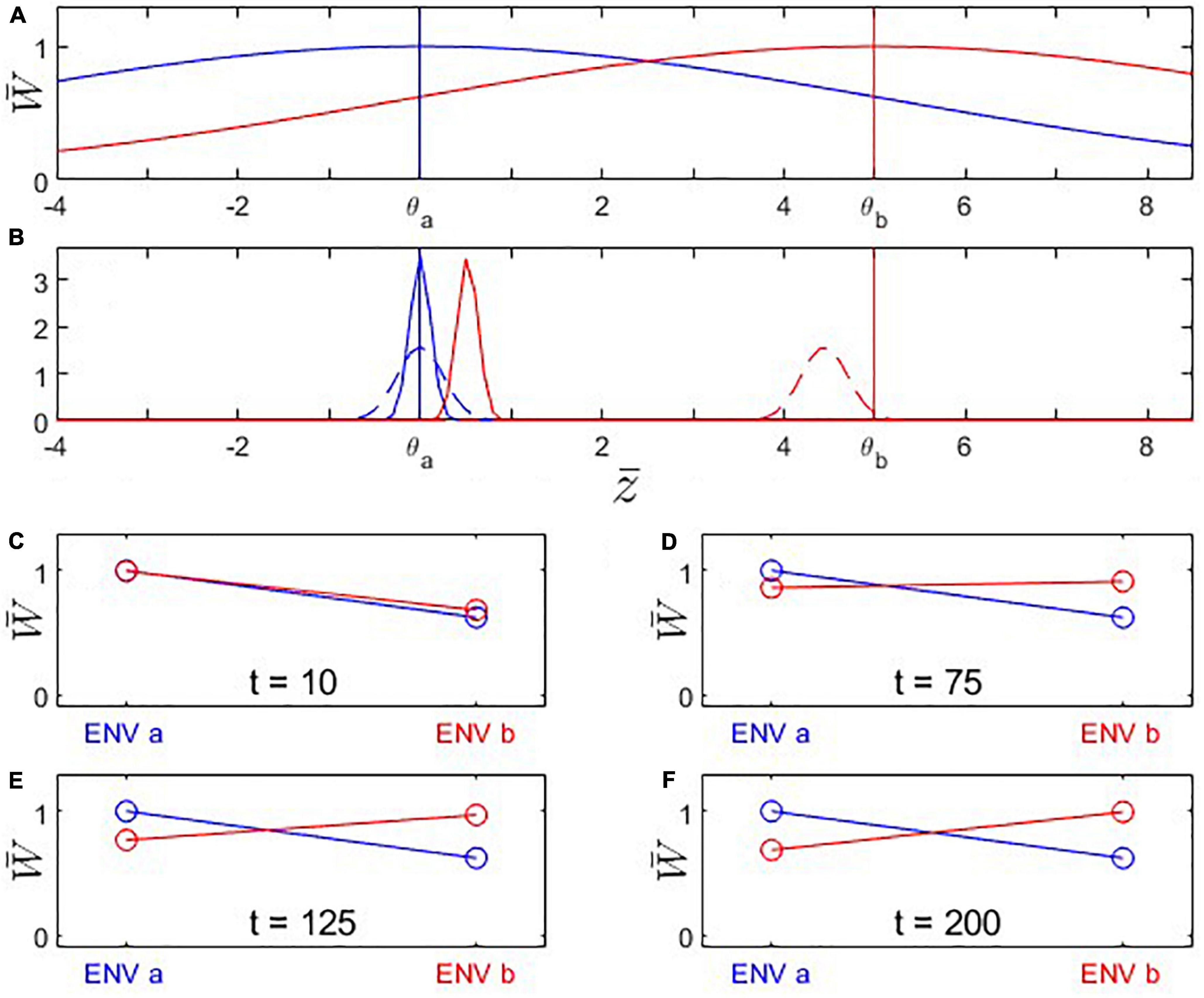
Figure 1. Fitness landscapes, trait evolution, and reciprocal-transplant experiments under Scenario 1: Trait optima are stationary; initial trait value ${\overline{z}}_0$ is located at the fitness optimum for environment a. Population B branches off from population A at time t₀ and adapts to the new environmental conditions dictated by the changed fitness landscape. (A) Fitness landscapes for environment a (blue) and b (red); vertical lines indicate the location of the fitness optima. (B) Probability distributions for phenotypic means after t = 10 (solid) and 200 (dashed) generations of evolution. Note that population A’s (blue) mean trait value remains in place while population B evolves toward the new trait optimum θ_b = 5. Also note that the width of the distribution shown is the variance of the mean phenotype across hypothetical replicated populations (arising due to genetic drift), not the genetic variance of a single population (which is assumed to remain constant). (C–F) Fitness plots for hypothetical reciprocal transplant experiments performed at t = 10, 75, 125, 200 (Left side of each panel: fitness of populations A (blue) and B (red) in environment a; right side: fitness of populations A and B in environment b). Parameters: ${\overline{z}}_{0,a}={\overline{z}}_{0,b}=0$; θ_a = 0; θ_b = 5; ${\overline{W}}_{\max ,a}={\overline{W}}_{\max ,b}=1$; ω_a = ω_b = 5; σ_a = σ_b = 1.135; $h_a^2=h_b^2=0.224$; N_a = N_b = 200.

FIGURE 2

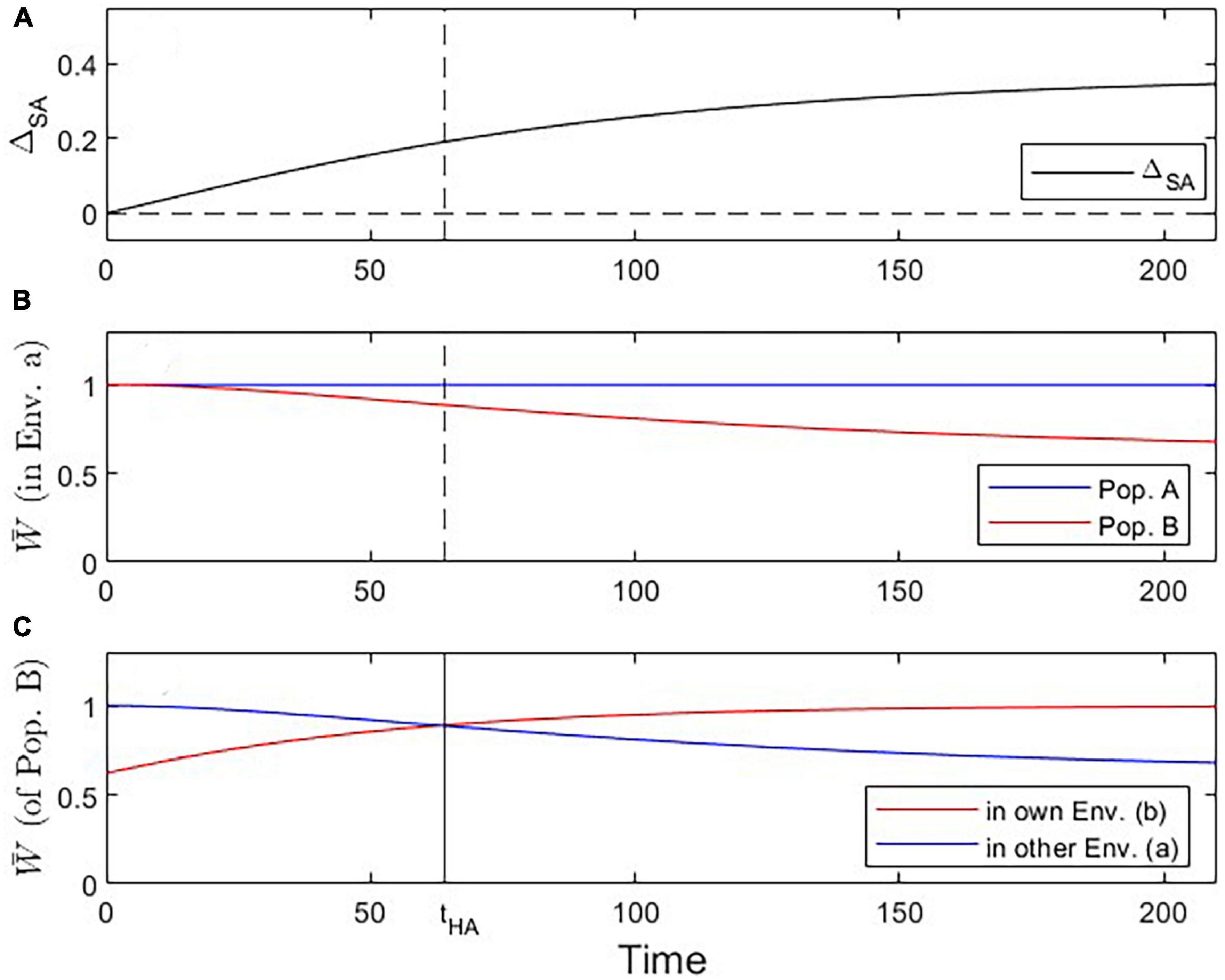
Figure 2. Visualization of three critical checkpoints during the evolutionary dynamics under Scenario 1. (A) Evidence for local adaptation by the Δ_SA contrast criterion (satisfied for all t > 0). (B) Fitness of population A vs. B in environment a (addressing the Local vs. Foreign criterion; satisfied for all t > 0). (C) Fitness of population B in own vs. other environment (addressing the Home vs. Away criterion; t_crit = 64; solid vertical line in this panel; dashed vertical line in other panels).

FIGURE 3

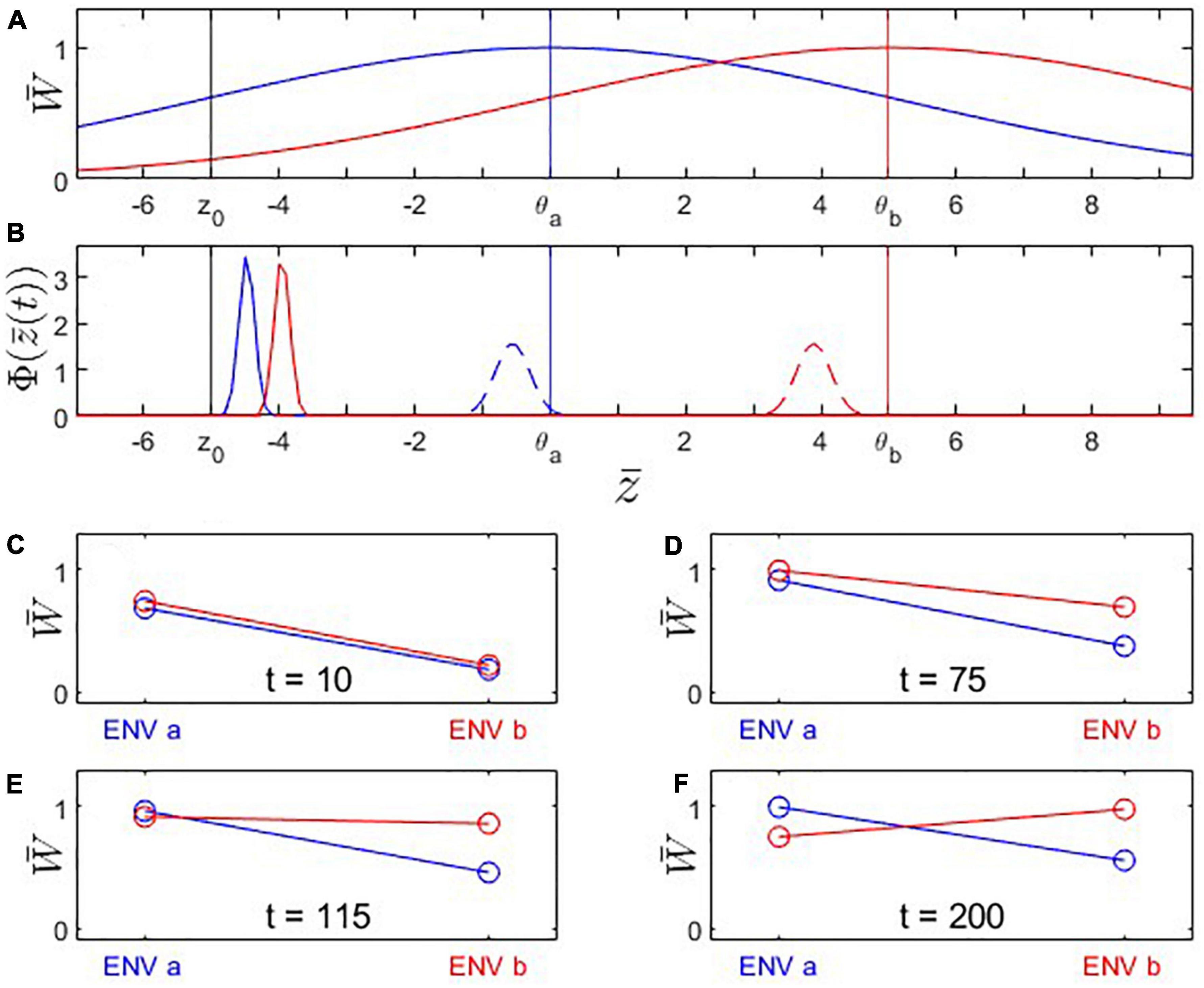
Figure 3. Fitness landscapes, trait evolution and reciprocal transplant experiments under Scenario 2: Trait optima are stationary; initial trait value ${\overline{z}}_0$ is located at a suboptimal value to the left of the fitness optimum for environment a. Both populations adapt to new environmental conditions but population B’s (red) fitness optimum is farther to the right than population A’s (blue). (A) Fitness landscapes for population A (blue) and population B (red); vertical lines: fitness optima (blue, red) and initial trait value ${\overline{z}}_0$ (black). (B) Distributions of phenotypic mean after t = 10 (solid) and t = 200 (dashed) generations of evolution. Note that population A’s (blue) mean trait value changes less than population B’s. (C–F) Fitness plots for hypothetical reciprocal transplant experiments performed at t = 10, 75, 115, 200. Parameters: ${\overline{z}}_{0,a}={\overline{z}}_{0,b}=-5$; other parameters as in Figure 1.

FIGURE 4

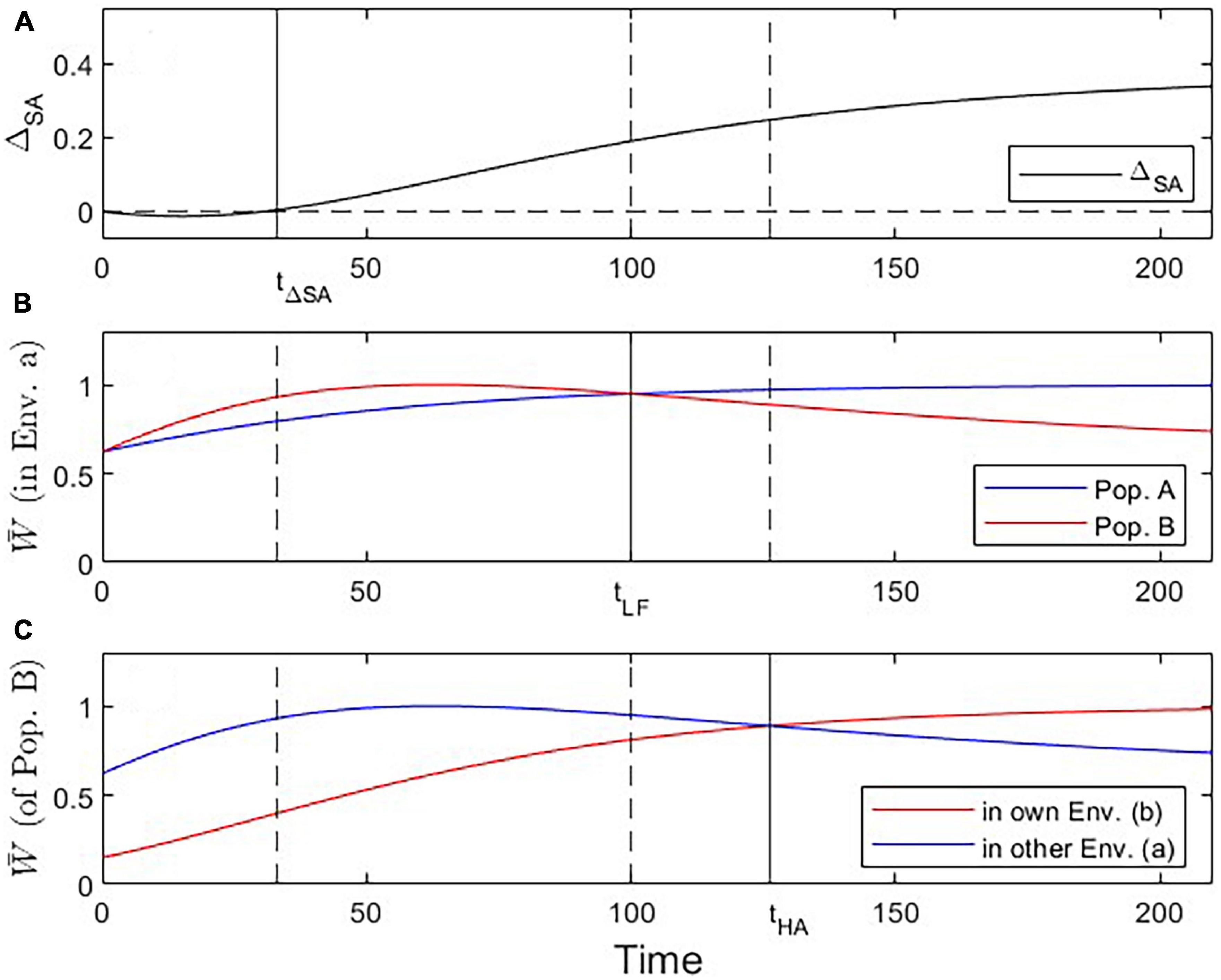
Figure 4. Visualization of three critical checkpoints (vertical lines) during the evolutionary dynamics under Scenario 2. (A) Evidence for adaptation by the Δ_SA contrast criterion (at t ≥ 33). (B) Fitness of population A vs. B in environment a (addressing the Local vs. Foreign criterion; t_crit = 100). (C) Fitness of Population B in own vs. other environment (addressing the Home vs. Away criterion; t_crit = 126).

2.2.2. Moving trait optima

Secondly, we analyze the more general case where the trait optima are gradually shifting over time in one direction (Scenario 3; Figures 5–7). Here, fitness differences will arise because, starting from the branching point, the two populations are facing environmental change that progresses at different speeds. The scenario is closely related to global-change phenomena (such as increasing temperatures), which are nearly ubiquitous but differ in magnitude regionally.

FIGURE 5

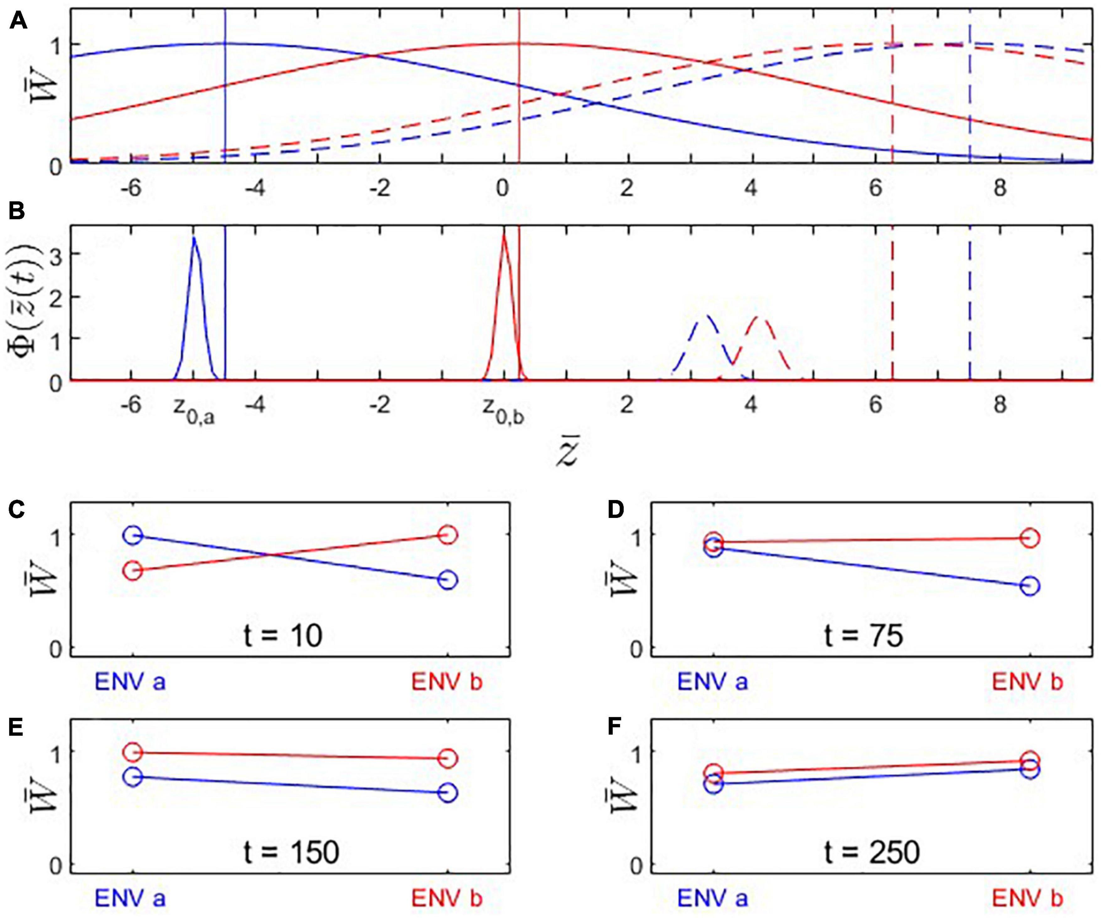
Figure 5. Fitness landscapes, trait evolution and reciprocal transplant experiments under Scenario 3: Trait optima are moving (from left to right along the x-axis); initial trait values ${\overline{z}}_{0,a}$ and ${\overline{z}}_{0,b}$ are located at the fitness optima for their environments. Both populations adapt to the shifting environmental conditions but population A’s (blue) fitness optimum moves faster than population B’s (red). (A) Fitness landscapes for population A (blue) and population B (red) at t = 10 (solid) and t = 250 (dashed); vertical lines: fitness optima. (B) Distributions of phenotypic means at t = 10 (solid) and t = 250 (dashed). Note that both populations are trailing their respective fitness optima. (C–F) Fitness plots for hypothetical reciprocal transplant experiments performed at t = 10, 75, 150, 250. Parameters: k_a = 0.050; k_b = 0.025; ${\overline{z}}_{0,a}=-5$; ${\overline{z}}_{0,b}=0$; other parameters as in Figure 1.

FIGURE 6

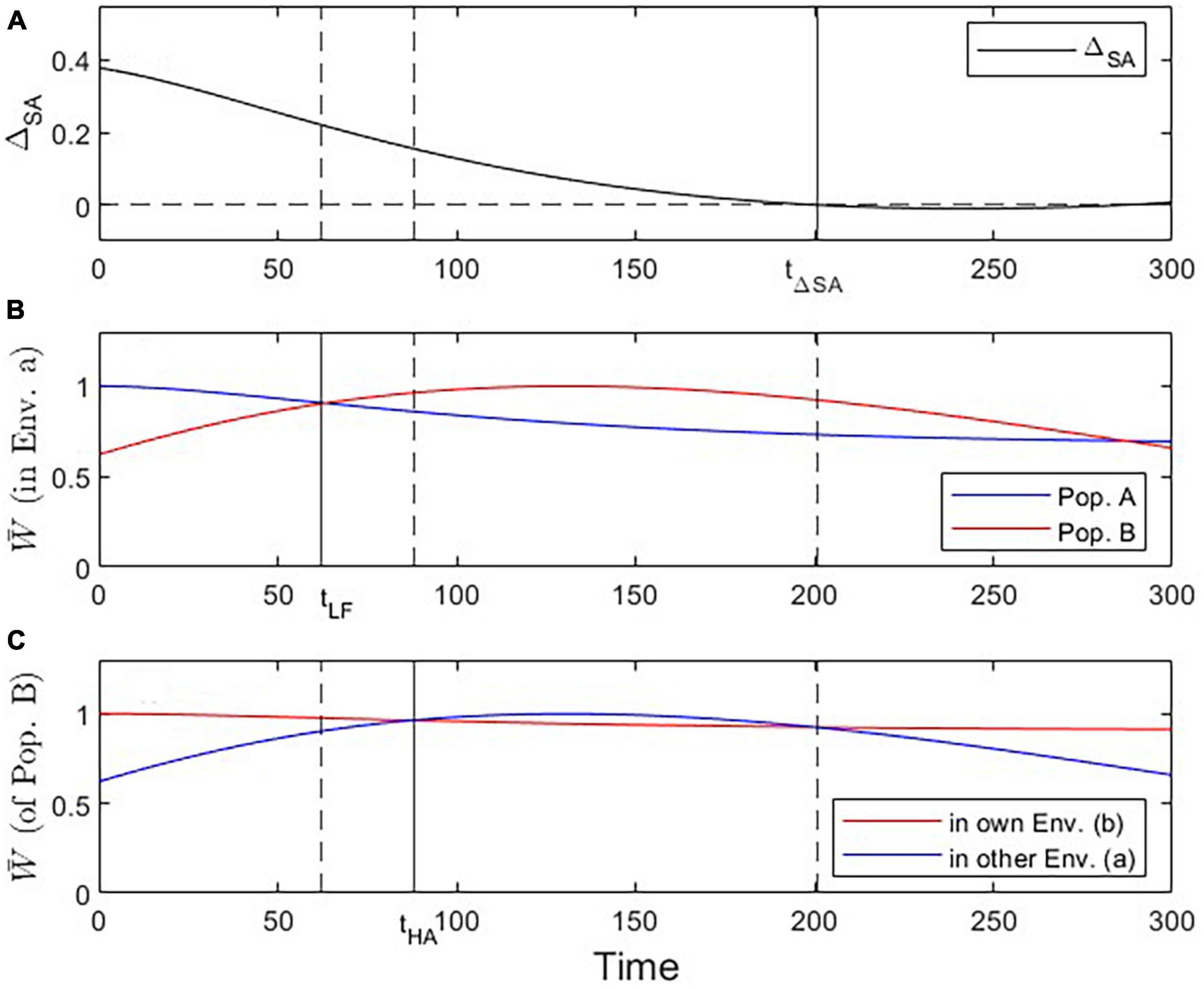
Figure 6. Visualization of three critical checkpoints (vertical lines) during the evolutionary dynamics under Scenario 3. (A) Evidence for local adaptation by the Δ_SA contrast criterion (at t ≤ 201). (B) Fitness of population A vs. B in environment a (addressing the Local vs. Foreign criterion; t_crit = 62). (C) Fitness of population B in own vs. other environment (addressing the Home vs. Away criterion; t_crit = 88).

FIGURE 7

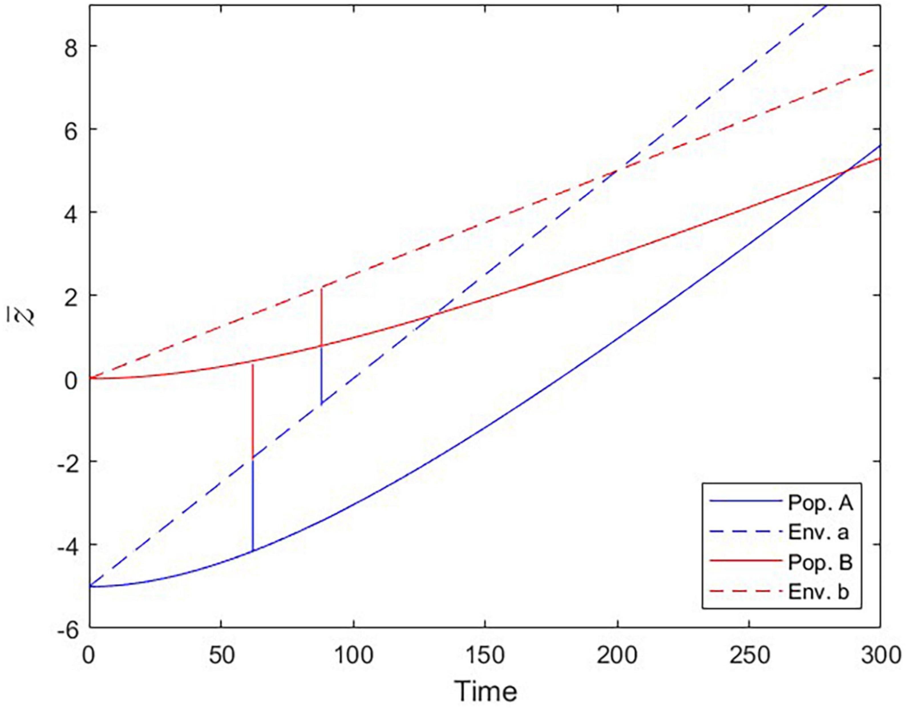
Figure 7. Populations trailing the moving fitness optima over time (Scenario 3). Optimal trait values set by the environmental conditions (dashed lines) and trait values realized by populations A and B (solid lines). At the Local vs. Foreign criterion checkpoint (t_crit = 62), population B is as fit in environment a as population A is. At the Home vs. Away criterion checkpoint (t_crit = 88), population B is equally fit in environments a and b.

Under this scenario, the trait optima of populations A and B start at the identical initial value θ₀ and move over time in the same direction, according to θ_t = kt, but at different rates k_a and k_b. The expected mean trait value ${\overline{z}}_{\mathrm{\Phi }}(t)$ of a population adapting to such a moving optimum is given by Estes and Arnold (2007):

${\overline{z}}_{\mathrm{\Phi }}(t)=\left(z_0+kt\right)-k\left(\frac{{\mathrm{\omega }}^2+{\mathrm{\sigma }}^2}{h^2{\mathrm{\sigma }}^2}\right)\left(1-\exp \left(-\frac{h^2{\mathrm{\sigma }}^2}{{\mathrm{\omega }}^2+{\mathrm{\sigma }}^2}t\right)\right),(3)$

with the same variance as in Equation 2.

2.3. Inference from reciprocal transplants

Different measures have been proposed to estimate local adaptation from the results of reciprocal transplant experiments (Kawecki and Ebert, 2004; Blanquart et al., 2013). A straightforward approach is to rely on estimates of the average local adaptation. For this measure, the Δ_SA contrast (i.e., sympatric vs. allopatric contrast), one calculates the difference between the average fitness in sympatric combinations of populations and sites and the average fitness in allopatric combinations (Blanquart et al., 2013), i.e., for our case of two populations A, B in two environments a, b:

${\mathrm{\Delta }}_{SA}=\frac{1}{2}\left({\overline{W}}_{Aina}+{\overline{W}}_{Binb}\right)-\frac{1}{2}\left({\overline{W}}_{Ainb}+{\overline{W}}_{Bina}\right),(4)$

where ${\overline{W}}_{J\text{in}i}$ is the average fitness of population J = A,B evaluated in environment i = a,b, respectively. Local adaptation would be indicated ifΔ_SA > 0.

In contrast, the Local vs. Foreign criterion (L–F) emphasizes the comparison between populations within environments (Kawecki and Ebert, 2004). Under local adaptation, the local population is expected to show higher fitness than the foreign population in both environments. This means that, in a classical reciprocal transplant plot, with environments on the x-axis and fitness on the y-axis, the lines connecting the fitness values of a given population in the two environments need to cross (as, e.g., in Figure 3E) (We note that, while it is also possible for the lines to cross if, in each environment, it is the foreign population that has higher fitness, such a case of complete maladaptation did not occur in our present study).

Finally, the Home vs. Away criterion (H-A) emphasizes the comparison between populations across environments (Kawecki and Ebert, 2004). Under this criterion, local adaptation exists if each population has higher fitness in its own environment than in the alternative environment. With respect to a reciprocal transplant plot, this means that local adaptation occurs if the line connecting the two fitness values for a population has a negative slope for population A and a positive slope for population B (assuming that environment a is placed to the left of environment b on the plot’s x-axis; as, e.g., in Figure 5D). Note that, under this criterion, no direct comparison is made between the fitness values of the two populations, however it is possible that one population is locally adapted to its environment while the other one is not.

3. Results

3.1. Stationary trait optima

We first analyze the most basic case (Scenario 1 above) where population A is perfectly adapted to its environment a, and population B branches off from population A and shows steady evolutionary adaptation toward a new optimal trait value in environment b (Figure 1). Reciprocal transplant experiments performed at different time points would show accumulating evidence of local adaptation (Figures 1C–F, 2). At t > 0, blue and red lines cross over, indicating that each population is fitter in its own environment than the other population (L-F criterion satisfied; Figure 2B). Once the mean trait value of Population B has evolved to be closer to the optimal trait value for environment b than the one for environment a, each population has higher fitness in its own environment than in the other environment (blue line has negative slope, red line has positive slope; H-A criterion satisfied; Figure 2C). Signal strength in support for both the L-F and H-A criteria increases with time, and so does the estimate of the average local adaptation, the Δ_SA contrast, which has a positive value at all times t > 0 (Figure 2A).

Under Scenario 2, both populations start the evolutionary process at a trait value displaced to the left of the optimal trait value for environment a (Figure 3A). Because population B’s trait optimum lies further to the right than that of population A, its evolutionary trajectory moves across high-fitness regions of population A’s fitness landscape. As a result, population B encounters periods where it is better adapted to environment a than population A, as well as periods where population B is better adapted to environment a than to environment b. Initially, none of the criteria for local adaptation is satisfied; with progressing evolution, however, the Δ_SA contrast, the L-F criterion, and the H-A criterion become consecutively fulfilled (Figure 4). Due to these periods of apparent maladaptation, hypothetical reciprocal transplant experiments would only reveal an unequivocal signature of local adaptation about 126 generations after the split of populations A and B (with the current parameterization; Figures 3F, 4C).

3.2. Moving trait optima

The phenomenon of apparent maladaptation also arises under Scenario 3 (moving trait optima with different speed). Because the conditions are assumed to be changing more rapidly in environment a than in environment b, population A is trailing the optimal trait value more than population B is. Starting from an initial state of complete local adaptation (Figures 5B, C), population B first gains fitness superiority over population A in environment a (loss of local adaptation according due to the L-F criterion; Figures 5D, 6B, 7), then population B becomes the universally more fit population (Figure 5E), and finally, population A becomes better adapted to environment b than to environment a, (loss of local adaptation according to the H-A criterion; Figures 5F, 6C, 7). If environmental and evolutionary change continue for a sufficiently long period, both populations will trail their environmental fitness optima by a constant gap (Figure 7), and the signature of relative (yet, not complete) local adaptation becomes reinstated (t ≈ 300).

4. Discussion

In this theoretical study we analyzed realistic evolutionary scenarios during which populations can display transitional fitness states that carry the signature of non-adaptation or maladaptation. Before discussing the implications of our findings in more detail, we feel that it is useful to evoke two conceptual perspectives: the concept of adaption as a process vs. adaptation as a state; and the concept of relative vs. absolute fitness.

Unlike evolution, which always refers to a process, adaptation can either refer to the process of adapting or to the state of being adapted. This distinction is very much at the core of our seemingly paradoxical observations, where populations strictly obey the laws of quantitative genetics by displaying monotonous adaptive evolution [i.e., they climb their respective adaptive hills, leading to “adaptive divergence” (Hendry, 2017)] yet undergo transient maladaptive states. Keeping the two views on adaptation straight is key when interpreting the kind of evolutionary dynamics that occurred in our study. However, we believe that we are dealing with a problem that runs deeper than merely a semantic issue. The reason is that nearly all practical methods of assessing adaptation in nature (such as reciprocal transplant or common garden experiments) implicitly quantify adaptive states, but the results are often interpreted as evidence for the process of evolutionary adaptation (or the lack thereof).

In a similar vein, distinguishing between relative and absolute fitness is crucial when discussing (mal)adaptation (Holt and Gomulkiewicz, 1997; Brady et al., 2019b). Specifically, evolutionary biologists tend to emphasize relative fitness while ecologists focus on absolute fitness (Hendry and Gonzalez, 2008; Brady et al., 2019b). This means that, to an evolutionary biologist who strictly applies the relative fitness concept, a population is maladapted if it has lower fitness than a relevant reference population. By contrast, an ecologist might score the same population as well adapted if it displays a positive growth rate in its local environment, and particularly so if the population has evolved toward this state from a previous state of lower absolute fitness. In our study, populations always increase their local absolute fitness in the environment they are adapting to (in Scenarios 1 and 2), except in cases where environmental change outpaces the capacity for evolutionary change (in some instances of Scenario 3). Relative fitness of a population, however, depends on the comparison with a reference population, either within (L-F criterion) or across (H-A criterion) environments.

Equipped with this background it should be straightforward to understand the evolutionary dynamics presented in Scenarios 2 and 3 for what they are, namely adaptive trajectories that, on their way to an adaptive steady state, pass through transient states of maladaptation (in the evolutionary sense above, that is in terms of relative fitness). This phenomenon can only occur while the evolutionary process is not at a (stable or dynamic) equilibrium, either because the populations are not initially at their fitness optima (Scenario 2) or because the fitness optima themselves are moving targets (Scenario 3; we also have analyzed the combination of these two causes of steady-state divergence but omitted the results from this paper as they did not provide any additional insights to what is presented here). The phenomenon necessarily implies change in relative fitness and may (Scenario 3) or may not (Scenario 2) be accompanied by intermittent loss of absolute fitness of one or both populations. The label “apparent maladaptation” (Brady et al., 2019b) tries to reconcile the facts that the underlying process is truly adaptive yet produces snapshots of true maladaptive states.

Our study has some implications for the interpretation of reciprocal transplant experiments, one of the primary methods for detecting and quantifying adaptive divergence (Kawecki and Ebert, 2004; Hendry, 2017). While many such experiments have detected clear patterns of local adaptation (Nagy, 1997; Hargreaves and Eckert, 2019), other studies have reported a nearly complete lack of adaptation (Low-Decarie et al., 2013; Rolshausen et al., 2015); indeed, meta-analyses have revealed that about 30% of experiments failed to detect the classical signature of local adaptation, i.e., higher relative fitness of local types in each environment (i.e., the L-F criterion) (Leimu and Fischer, 2008; Hereford, 2009). Part of these results are likely due to a lack of adaptive dynamics per se (e.g., due to lack of genetic variation). In addition, however, our study points to a variety of cases that fail to produce adaptive signatures even in the presence of adaptive dynamics, leading to apparent maladaptation. These cases include examples of one population being relatively better locally adapted than the other, no matter what the environment (e.g., Figures 3C, D, 5D–F); or examples of one environment leading to lower absolute fitness of both populations than the other environment (e.g., Figures 3C–E), even with the identity of the low-fitness environment switching over time (Figures 5E, F). That said, we did not find any instances of complete maladaptation, where each population has the highest fitness in the non-native environment. In a real experimental situation, maladaptive patterns of the kind we observed may arise due to a multitude of factors such as constraints on evolution, genotype-by-environment interaction, co-evolution, unaccounted traits under selection or phenotypic plasticity (Bjorklund, 1996; Hendry, 2017). We would like to add to this list as a possible factor “transient adaptive dynamics,” given that our results demonstrate that these trajectories do not just amount to a delayed approach to the adaptive state (as in Scenario 1) but may cross through truly maladaptive transition states (Scenarios 2, 3). This realization is very much in line with the idea and recent experimental demonstration of an “adaptational lag” (akin to our Scenario 3) that leads to fitness superiority of non-native populations because local populations failed to keep evolutionary pace with rapid environmental climate change (Kooyers et al., 2019). Reciprocal transplants are often labor-intensive experiments, replication in time (as simulated in our purposefully placed snapshots presented in panels C through F of Figures 1, 3, 5) is rarely possible, and the evolutionary history of the populations chosen for the experiment is often scarcely known. As such, we advise against taking the absence of evidence for adaptation (based on results from a single reciprocal transplant or common garden experiment) as hard evidence for the absence of adaptive divergence.

Over the course of the adaptive divergence observed in our model simulations, we were able to track certain measures commonly used as indicators of local adaptation (see Section 2.3). Among these measures, the Local vs. Foreign criterion (L-F) adopts the most “evolutionary” perspective, in that it emphasizes the comparison of relative fitness among populations, and some authors maintain that it should be used as the only diagnostic for establishing local adaptation (Kawecki and Ebert, 2004). An implicit consequence of the L-F criterion is that overall local adaptation can only be concluded from a reciprocal transplant experiment if all populations tested are locally adapted. Other authors found this criterion overly strict and impractical and have advocated for adopting the Δ_SA contrast, which is satisfied if, on average, populations have higher fitness in their native than in their non-native environments (Blanquart et al., 2013). Which criterion a researcher decides to use when interpreting their experiment probably depends ultimately on the experimental design and the type and strength of inference they wish to draw from their experiment. We feel, that, in our study, the Δ_SA contrast proved to be an unacceptably lenient benchmark. For instance, this criterion would have led us to conclude local adaptation in the cases depicted in Figures 3D or 5E, simply based on the fact that the adaptation of population B to environment b slightly exceeds the clear maladaptation of Population A to environment a. In situations like ours, where only few populations and environments are compared with one another, the L-F and H-A criteria appear to be the more useful diagnostics. In all our simulations, both diagnostics were far more restrictive in assigning local adaptation to results of a reciprocal transplant experiment than the Δ_SA contrast; however, which of the two measures (L-F or H-A) were satisfied during a longer period of the simulated evolutionary dynamics depended on the concrete parameterization.

We framed our study around populations that face different adaptive challenges for a certain period of time and whose local fitnesses are compared afterwards in the context of a reciprocal transplant experiment. One could argue that this scenario has similarities with the process of species invasions that occur on a global scale, even more so because it is becoming increasingly clear that climate change can be a crucial factor determining the introduction and establishment of non-native species (Hulme, 2017; Ricciardi et al., 2021). Hence, our Scenario 3 could also be interpreted from an invasion biological perspective, where trait optima shift due to the regionally different intensity and speed of climate change. Our current approach is certainly too generic in parameterization as well as too low-dimensional in trait space to be able to make useful predictions for concrete invasion scenarios. However, we would like to point out the possibility that the L-F and H-A checkpoints might serve as invasion criteria. Over the course of adaptation to climate change a potentially invasive species would likely increase its invasion potential in two steps. It would (a) develop higher relative fitness than the resident species and (b) become better adapted to the foreign environment than to its native environment (Figure 7). Checkpoint a aligns with the L-F criterion and gives the invader the competitive edge, whereas checkpoint b (= H-A) would increase the incentive to migrate out of the native environment (provided there are individuals that are able to probe both environments as, for instance, in migratory birds). Our simulations revealed that the order in which these two events occur is not fixed and depends on the specific conditions (i.e., parameterizations, in the model), but they always occurred in temporal succession. It would be premature to decide if one of the two criteria can serve as a more significant predictor for invasion success than the other, but in many real-life scenarios the invasion probability will likely be higher when both criteria are met.

In this theoretical study we have elaborated on the phenomenon of apparent maladaptation that previously has been sketched out in Brady et al. (2019b). We have shown that our results have potentially important implications in applied areas that reach beyond theoretical evolutionary biology. However, we also decided to keep things simple, traceable and generic by using a very simple evolutionary model that was not parameterized for any concrete real eco-evolutionary scenario. We consider our contribution a first step toward investigating this interesting phenomenon of apparent maladaptation. We can envision many realistic model alterations, such as multiple evolving traits, evolutionary constraints, alternatively shaped fitness functions (Osmond and Klausmeier, 2017), eco-evolutionary scenarios in multi-species communities (Govaert et al., 2019; Hui et al., 2021), and so on, and invite other researchers to evaluate the validity of our conclusions under model realizations that mirror more concrete scenarios than we were able to analyze.

Data availability statement

The original contributions presented in this study are included in the article/Supplementary material, further inquiries can be directed to the corresponding author.

Author contributions

GF conceived the study, performed the modeling, and wrote the first draft of the manuscript. MK performed the analyses presented in the Supplementary material. Both authors analyzed and interpreted the results, discussed the scope of the manuscript, edited the manuscript, and approved the final version.

Funding

GF was supported by NSERC Discovery Grant RGPIN/04780-2020.

Acknowledgments

GF is grateful for a sabbatical leave granted by McGill University, which promoted the research collaboration leading to this publication.

Conflict of interest

The authors declare that the research was conducted in the absence of any commercial or financial relationships that could be construed as a potential conflict of interest.

Publisher’s note

All claims expressed in this article are solely those of the authors and do not necessarily represent those of their affiliated organizations, or those of the publisher, the editors and the reviewers. Any product that may be evaluated in this article, or claim that may be made by its manufacturer, is not guaranteed or endorsed by the publisher.

Supplementary material

The Supplementary Material for this article can be found online at: https://www.frontiersin.org/articles/10.3389/fevo.2023.1151283/full#supplementary-material

References

Bennett, J. M., Sunday, J., Calosi, P., Villalobos, F., Martinez, B., Molina-Venegas, R., et al. (2021). The evolution of critical thermal limits of life on earth. Nat. Commun. 12:1198. doi: 10.1038/s41467-021-21263-8

PubMed Abstract | CrossRef Full Text | Google Scholar

Bjorklund, M. (1996). The importance of evolutionary constraints in ecological time scales. Evol. Ecol. 10, 423–431. doi: 10.1007/Bf01237727

CrossRef Full Text | Google Scholar

Blanquart, F., Kaltz, O., Nuismer, S. L., and Gandon, S. (2013). A practical guide to measuring local adaptation. Ecol. Lett. 16, 1195–1205. doi: 10.1111/ele.12150

PubMed Abstract | CrossRef Full Text | Google Scholar

Brady, S. P., Zamora-Camacho, F. J., Eriksson, F. A. A., Goedert, D., Comas, M., and Calsbeek, R. (2019c). Fitter frogs from polluted ponds: The complex impacts of human-altered environments. Evol. Appl. 12, 1360–1370. doi: 10.1111/eva.12751

PubMed Abstract | CrossRef Full Text | Google Scholar

Brady, S. P., Bolnick, D. I., Angert, A. L., Gonzalez, A., Barrett, R. D. H., Crispo, E., et al. (2019a). Causes of maladaptation. Evol. Appl. 12, 1229–1242. doi: 10.1111/eva.12844

PubMed Abstract | CrossRef Full Text | Google Scholar

Brady, S. P., Bolnick, D. I., Barrett, R. D. H., Chapman, L., Crispo, E., Derry, A. M., et al. (2019b). Understanding maladaptation by uniting ecological and evolutionary perspectives. Am. Nat. 194, 495–515. doi: 10.1086/705020

PubMed Abstract | CrossRef Full Text | Google Scholar

Bürger, R., and Lynch, M. (1995). Evolution and extinction in a changing environment - a quantitative-genetic analysis. Evolution 49, 151–163. doi: 10.2307/2410301

CrossRef Full Text | Google Scholar

Deutsch, C. A., Tewksbury, J. J., Huey, R. B., Sheldon, K. S., Ghalambor, C. K., Haak, D. C., et al. (2008). Impacts of climate warming on terrestrial ectotherms across latitude. Proc. Natl Acad. Sci. U.S.A. 105, 6668–6672. doi: 10.1073/pnas.0709472105

PubMed Abstract | CrossRef Full Text | Google Scholar

Diamond, S. E. (2018). Contemporary climate-driven range shifts: Putting evolution back on the table. Funct. Ecol. 32, 1652–1665. doi: 10.1111/1365-2435.13095

CrossRef Full Text | Google Scholar

Estes, S., and Arnold, S. J. (2007). Resolving the paradox of stasis: Models with stabilizing selection explain evolutionary divergence on all timescales. Am. Nat. 169, 227–244. doi: 10.1086/510633

PubMed Abstract | CrossRef Full Text | Google Scholar

Fraser, D. J., Walker, L., Yates, M. C., Marin, K., Wood, J. L. A., Bernos, T. A., et al. (2019). Population correlates of rapid captive-induced maladaptation in a wild fish. Evol. Appl. 12, 1305–1317. doi: 10.1111/eva.12649

PubMed Abstract | CrossRef Full Text | Google Scholar

Govaert, L., Fronhofer, E. A., Lion, S., Eizaguirre, C., Bonte, D., Egas, M., et al. (2019). Eco-evolutionary feedbacks-theoretical models and perspectives. Funct. Ecol. 33, 13–30. doi: 10.1111/1365-2435.13241

CrossRef Full Text | Google Scholar

Hargreaves, A. L., and Eckert, C. G. (2019). Local adaptation primes cold-edge populations for range expansion but not warming-induced range shifts. Ecol. Lett. 22, 78–88. doi: 10.1111/ele.13169

PubMed Abstract | CrossRef Full Text | Google Scholar

Hendry, A. P. (2017). Eco-evolutionary dynamics. Princeton, NJ: Princeton University Press.

Google Scholar

Hendry, A. P., and Gonzalez, A. (2008). Whither adaptation? Biol. Philos. 23, 673–699. doi: 10.1007/s10539-008-9126-x

CrossRef Full Text | Google Scholar

Hereford, J. (2009). A quantitative survey of local adaptation and fitness trade-offs. Am. Nat. 173, 579–588. doi: 10.1086/597611

PubMed Abstract | CrossRef Full Text | Google Scholar

Holt, R. D., and Gomulkiewicz, R. (1997). How does immigration influence local adaptation? A reexamination of a familiar paradigm. Am. Nat. 149, 563–572. doi: 10.1086/286005

CrossRef Full Text | Google Scholar

Hui, C., Richardson, D. M., Landi, P., Minoarivelo, H. O., Roy, H. E., Latombe, G., et al. (2021). Trait positions for elevated invasiveness in adaptive ecological networks. Biol. Invas. 23, 1965–1985. doi: 10.1007/s10530-021-02484-w

CrossRef Full Text | Google Scholar

Hulme, P. E. (2017). Climate change and biological invasions: Evidence, expectations, and response options. Biol. Rev. 92, 1297–1313. doi: 10.1111/brv.12282

PubMed Abstract | CrossRef Full Text | Google Scholar

Kawecki, T. J., and Ebert, D. (2004). Conceptual issues in local adaptation. Ecol. Lett. 7, 1225–1241. doi: 10.1111/j.1461-0248.2004.00684.x

CrossRef Full Text | Google Scholar

Kooyers, N. J., Colicchio, J. M., Greenlee, A. B., Patterson, E., Handloser, N. T., and Blackman, B. K. (2019). Lagging adaptation to climate supersedes local adaptation to herbivory in an annual monkeyflower. Am. Nat. 194, 541–557. doi: 10.1086/702312

PubMed Abstract | CrossRef Full Text | Google Scholar

Kopp, M., and Matuszewski, S. (2014). Rapid evolution of quantitative traits: Theoretical perspectives. Evol. Appl. 7, 169–191. doi: 10.1111/eva.12127

PubMed Abstract | CrossRef Full Text | Google Scholar

Lande, R. (1976). Natural selection and random genetic drift in phenotypic evolution. Evolution 30, 314–334. doi: 10.2307/2407703

CrossRef Full Text | Google Scholar

Leimu, R., and Fischer, M. (2008). A Meta-Analysis of Local Adaptation in Plants. PLoS One 3:e4010. doi: 10.1371/journal.pone.0004010

PubMed Abstract | CrossRef Full Text | Google Scholar

Loria, A., Cristescu, M. E., and Gonzalez, A. (2019). Mixed evidence for adaptation to environmental pollution. Evol. Appl. 12, 1259–1273. doi: 10.1111/eva.12782

PubMed Abstract | CrossRef Full Text | Google Scholar

Low-Decarie, E., Jewell, M. D., Fussmann, G. F., and Bell, G. (2013). Long-term culture at elevated atmospheric CO₂ fails to evoke specific adaptation in seven freshwater phytoplankton species. Proc. R. Soc. B Biol. Sci. 280:20122598. doi: 10.1098/rspb.2012.2598

PubMed Abstract | CrossRef Full Text | Google Scholar

Nagy, E. S. (1997). Selection for native characters in hybrids between two locally adapted plant subspecies. Evolution 51, 1469–1480. doi: 10.2307/2411199

CrossRef Full Text | Google Scholar

Osmond, M. M., and Klausmeier, C. A. (2017). An evolutionary tipping point in a changing environment. Evolution 71, 2930–2941. doi: 10.1111/evo.13374

PubMed Abstract | CrossRef Full Text | Google Scholar

Ricciardi, A., Iacarella, J. C., Aldridge, D. C., Blackburn, T. M., Carlton, J. T., Catford, J. A., et al. (2021). Four priority areas to advance invasion science in the face of rapid environmental change. Environ. Rev. 29, 119–141. doi: 10.1139/er-2020-0088

CrossRef Full Text | Google Scholar

Rolshausen, G., Phillip, D. A. T., Beckles, D. M., Akbari, A., Ghoshal, S., Hamilton, P. B., et al. (2015). Do stressful conditions make adaptation difficult? Guppies in the oil-polluted environments of southern Trinidad. Evol. Appl. 8, 854–870. doi: 10.1111/eva.12289

PubMed Abstract | CrossRef Full Text | Google Scholar

Somero, G. N. (2010). The physiology of climate change: How potentials for acclimatization and genetic adaptation will determine ‘winners’ and ‘losers’. J. Exp. Biol. 213, 912–920. doi: 10.1242/jeb.037473

PubMed Abstract | CrossRef Full Text | Google Scholar

Sunday, J. M., Bates, A. E., and Dulvy, N. K. (2012). Thermal tolerance and the global redistribution of animals. Nat. Clim. Change 2, 686–690. doi: 10.1038/Nclimate1539

CrossRef Full Text | Google Scholar