A Dynamic Optimality Principle for Water Use Strategies Explains Isohydric to Anisohydric Plant Responses to Drought

1. Introduction

Some two centuries after the original experiments of Francis Darwin (Darwin, 1898; Scarth, 1927), the significance of stomatal kinetics in climate, atmospheric, hydrologic, agricultural, and ecosystem sciences is not in dispute (Hetherington and Woodward, 2003). The exchange of water vapor and CO₂ between the atmosphere and plants is regulated by a dynamic stomatal aperture. This impacts a plethora of processes such as CO₂ concentration in the atmosphere (c_a) and positive feedbacks on air temperature (Cox et al., 2000) as well as water cycling (Betts et al., 2007; Katul et al., 2012), sensible heat flux, and boundary layer dynamics regulating rainfall predisposition (Siqueira et al., 2009; Manoli et al., 2016). Other impacted processes also include pollutant uptake such as tropospheric ozone and concomitant plant damage (Rich, 1964; Musselman et al., 2006), antecedent soil moisture content and flash-flooding (Javelle et al., 2010), silviculture and forest management (Mäkelä and Hari, 1986), and irrigation water requirements and profitable crop yield estimation (Vico and Porporato, 2015) to name a few. What remains the subject of inquiry is how to represent stomatal kinetics for the above applications parsimoniously.

Numerous models for stomatal kinetics have emerged over the past century or so (for an overview see e.g., Jarvis, 1976; Collatz et al., 1991; Leuning, 1995; Damour et al., 2010; Way et al., 2011). These studies rely on two points. The first is that stomatal kinetics cannot be considered in isolation as they are impacted by exogenous environmental variables (Jarvis, 1976; Pearcy, 1990; Mott and Parkhurst, 1991; Medlyn et al., 2002) such as photosynthetically active radiation (PAR), air temperature (T_a), vapor pressure deficit (VPD), and c_a. This is in addition to the effects of endogenous variables impacted by soil-root-plant processes such as soil, rhizosphere, and plant hydraulics (Sperry, 2000; Brodribb et al., 2003), osmoregulation and carbohydrate export from the leaf (Nikinmaa et al., 2013; Sevanto et al., 2014; Jensen et al., 2016; Konrad et al., 2018) to name a few. The second point is that optimization approaches based on maximum fitness offer a whole-system framework to begin tackling the description of stomatal kinetics (Manzoni et al., 2011, 2013; Huang et al., 2018). Because photosynthesis is the main source of carbon used by plants for numerous functions such as growth and defenses (Novick et al., 2012), maximizing fitness is akin to maximizing photosynthesis over a preset time scale yet to be determined (Cowan and Troughton, 1971; Givnish and Vermeij, 1976; Cowan and Farquhar, 1977; Dewar, 2010). This approach is appealing because the mathematical framework to be employed (i.e., variational principles) has been used in numerous branches of science (Witelski and Bowen, 2015). The barriers of this approach are not in the formulation of the “functional” to be maximized (i.e., photosynthesis) but in the constraints and costs to be imposed on such an optimization (Dewar et al., 2018). Naturally, these constraints and costs operate over time scales that may be difficult to determine a priori. Early work relying on variational principles focused on maximizing photosynthesis by setting costs (in carbon units) as transpirational losses from leaves (Cowan and Farquhar, 1977; Cowan, 1978). Other versions of this approach maximize instantaneous carbon gain for a given finite amount of water loss per unit leaf area (Katul et al., 2009). A recent approach seeks instantaneous maximization of gains and assumes that plant hydraulics control stomatal opening trends. The approach is now labeled as a gain-risk or profit maximization model for stomatal kinetics (Sperry et al., 2016, 2017). The profit maximization scheme formulates the cost based on a relative loss in plant hydraulic conductance. Other optimization variants have also been proposed based on maintaining constant inter-cellular to ambient atmospheric CO₂ concentration ratio (Prentice et al., 2014) or maximizing carbon transport out of the leaves through the phloem (Nikinmaa et al., 2013). In the constant internal-to-ambient CO₂ concentration ratio approach, the objective is to minimize instantaneous cost (instead of maximizing gains) of maintaining the transpirational stream required to support photosynthesis while maintaining photosynthetic proteins at levels required to support assimilation rates. Predictions from all these approaches have received experimental support under wide-ranging conditions despite differences in formulating costs (Nikinmaa et al., 2013; Prentice et al., 2014; Sperry et al., 2017).

The past five decades have witnessed a renaissance in the development and use of optimization theories to describe stomatal kinetics. This renaissance led to the revision of the nature of the costs associated with photosynthetic gains to include soil-plant hydraulics, soil water availability, energy limitations (Roth-Nebelsick and Konrad, 2018) among others, and are all gaining prominence and partial experimental support. What is missing is a general framework that can (i) recover the various optimization schemes already proposed and (ii) explicitly link these schemes with plant water use strategies (WUS). This work interprets WUS as the relative importance prescribed to instantaneous vs. delayed gains. A conservative plant is one that prescribes more importance to delayed gains than a relatively aggressive one. This interpretation was first introduced mathematically elsewhere (Manzoni et al., 2013) and is built upon in the current article.

The work here aims to establish the blueprint of a calculus of variations based framework using plant hydraulics and droughts as case studies. The focus on droughts is purposeful because of the recent interest in plant-water use strategies during droughts, and ways of defining and measuring isohydricity (Franks et al., 2007; Martínez-Vilalta et al., 2014; Meinzer et al., 2016). Such analysis requires a re-formulation of the conventional optimization problem to satisfy all constraints at a sub-daily time scale while maximizing carbon gain over a dry-down period. A dry-down period is here defined as the period of time in between consecutive rainfall events. The multiplicity of time scales exists to both explicitly accommodate variable environmental drivers and abiotic (e.g., drainage) as well as biotic (i.e., overlapping rooting zones of adjacent plants) competition for water and optimize plant fitness (here seen as total carbon assimilated). The theoretical framework to be employed is based on the calculus of variations and dynamic optimization principles because they allow for (i) directly accounting for plant-water use strategies (i.e., aggressive vs. conservative water users), (ii) using multiple constraints (hydrologic balance, energy balance, etc…), and (iii) extending the deterministic analysis used here to a stochastic framework (at least for rainfall) using conventional approaches (Cowan, 1986; Mäkelä et al., 1996; Manzoni et al., 2013; Lu et al., 2016). Setting a “carbon value” to the terminal soil moisture content around the rooting zone at the end of the dry-down period allows mathematically assigning a plant water use strategy (Manzoni et al., 2013). The focus of the work here will be restricted to the aforementioned point (i) so as to demonstrate the utility of the proposed approach here and leave points (ii) and (iii) for future inquiry and extensions of the proposed method. It is not the goal of the current article to complexify the computational needs so as to achieve good agreement with a particular site or study. The main contribution here is the presentation of the mathematical machinery required to add plant hydraulic (and other) limitations to the traditional and widely used optimization principle for stomatal behavior (Cowan and Farquhar, 1977; Cowan, 1986). The optimization scheme developed by Cowan and Farquhar (1977) has been shown to perform well with data in the past (Dubois et al., 2007; Gu et al., 2010). The rest of the document will discuss what amendments are needed to extend this framework to drought studies. The approach will be compared with a controlled experiment (Venturas et al., 2018) that was used to test the gain-risk scheme.

As a guide to the development of this framework, the work answers the following question: To what degree does water use strategy dictate stomatal control during dry-down? In a recent review of the theory of optimal stomatal control, Buckley et al. (2017) emphasized the importance of delayed benefits such as keeping soil moisture at higher levels for future use, which is accommodated here using a terminal gain. The optimization scheme proposed explores the consequences of WUS and choices made about soil-plant hydraulic strategy, and whether few but important plant hydraulic traits alone are capable of mapping stomatal behavior anywhere on the iso-anisohydric spectrum. In particular, the model behavior is discussed in the water demand and supply limited cases to demonstrate the influence of competition on plant water use for trees of three different hydraulic vulnerability (to embolism) curves (VCs). Another point of departure from previous analyses based on treating g_s as the control variable is that soil-plant hydraulics limit plant transpiration when atmospheric water demand exceeds the supply of water provided by the soil and xylem. This limitation imposes an upper bound on g_s. The newly proposed model results are then compared with the recently developed gain-risk scheme (Venturas et al., 2018).

2. Materials and Methods

This section will first present a review of the calculus of variations applied to plant photosynthesis and then describe an alteration to mathematically formalize the concept of Water Use Strategy (WUS). The WUS concept recognizes that for the same plant hydraulic, allometric, and photosynthetic traits, a plant can adopt a spectrum of water use intensities varying from aggressive to conservative. The third sub-section relates carbon fixation to g_s and details the assumptions adopted. The fourth and fifth sub-sections develop conservation of water mass equations needed to obtain physically plausible results. The third and fifth sub-sections combined are the analytical basis of the carbon gain and water loss trade-off with stomatal opening. The sixth sub-section explains the mathematical machinery behind maximizing carbon gain while combining the objectives, formulations, and constraints developed in the previous sub-sections. The seventh sub-section details the gain-risk model used for comparison (Sperry and Love, 2015; Sperry et al., 2016). The eighth and final sub-section explains the values of parameters used, which species were modeled, and the test cases chosen to run the model.

2.1. Theory: Calculus of Variations

The principle adopted here is that plants maximize their carbon gain (A) over a dry-down period T selected to be the mean inter-storm period. This principle assumes that plants control g_s under constraints. Previous work constrained control of g_s by enforcing the daily water balance at the soil level (Manzoni et al., 2013). To mathematically express this principle under the mentioned constraint, an augmented Lagrangian is defined L:

$\begin{array}{ll}L(g_s,x,\frac{dx}{dt},\lambda ,t)=A(g_s,t)-\lambda [\frac{dx}{dt}-f_e(g_s,x,\frac{dx}{dt},t)],& (1)\end{array}$

where λ is the Lagrange multiplier in mol mol⁻¹ known as the instantaneous marginal water use efficiency in ecological terms; x is the relative soil moisture content or degree of saturation in the rooting zone bounded between zero (dry soil) and unity (all pores are filled with water) in m³ m⁻³; t is time in days; and f_e is the summation of all soil hydrological fluxes in days⁻¹.

Because the approach states that A is maximized over a period T rather than instantaneously, the objective function J integrates L from t = 0 signifying the beginning of a dry down to t = T at the end of it:

$\begin{array}{ll}J(g_s,x,\frac{dx}{dt},\lambda ,t)={\displaystyle {\int }_0^T}L(g_s,x,\frac{dx}{dt},\lambda ,t).& (2)\end{array}$

The goal then consists of finding the function g_s(t) in terms of t that maximizes J over the period T. This goal is achieved by solving the Euler-Lagrange equations using the calculus of variations (Witelski and Bowen, 2015). This approach requires expressing A and f_e as functions of the control variable g_s and the state variable x, which are now discussed. Again, while L is maximized over a drydown period T, g_s, x, its derivative, and λ are all resolved at sub-daily or diurnal time scale.

2.2. Water Use Strategy (WUS)

A terminal gain term is added to J to include the effects of water use strategy (WUS; Manzoni et al., 2013). The revised objective function J is now:

$\begin{array}{ll}{J}_{\text{WUS}}={\displaystyle {\int }_0^T}L(g_s,x,\frac{dx}{dt},\lambda ,t)dt+J_T,& (3)\end{array}$

where J_T is the terminal gain term. J_T may take different forms but should represent the costs of aggressively opening stomata regardless of drought. For simplicity, J_T may be interpreted as the carbon value of the terminal soil water moisture x(T) prescribed as:

$\begin{array}{ll}{J}_T=\Lambda x(T),& (4)\end{array}$

where the introduced parameter Λ in mol mol⁻¹ sets the carbon value of x(T). Larger Λ represents a more conservative WUS and vice versa (Manzoni et al., 2013). Ecologically, the terminal gain J_T as expressed in Equation (4) prevents excessive and detrimental use of water especially during a short dry-down period (i.e., small T). As will be shown in the “Maximizing the objective” sub-section below, the value of J_T, as expressed in Equation (4), can be inferred experimentally in water stressed environments by observing the marginal water use efficiency (λ) of a plant under dry soil.

The plant could now “maximize” its objective J_WUS by keeping a high x(T) at the end of dry-down. A higher x(T) means higher potential carbon gains after drought, limited loss in root to leaf hydraulic conductance, among other advantages. The magnitude of J_T should be interpreted with consideration of the length of the dry-down period (T). The same J_T contributes to a smaller portion of the objective function for a longer dry-down period (Equation 4). In this study, the length of the dry-down period is fixed across all experiments as it is presumed to be externally imposed on the soil-plant system by the precipitation regime. Future studies will assume this quantity randomly distributed set by the actual instead of the mean inter-storm period. Throughout, J_WUS will be the objective to be maximized instead of J of Equation (2).

2.3. Carbon Gain

The biochemical demand (A_demand) for atmospheric CO₂ for a C3 leaf is either limited by the Ribulose-1,5-bisphosphate carboxylase/oxygenase (Rubisco) enzyme activity under saturated incoming PAR or by Ribulose-1,5-biphosphate (RuBP) activity under limiting incoming PAR (Farquhar et al., 1980). To consider both limitations using a differentiable function that facilitates numerical optimization, A_demand is calculated using the co-limitation approach as (Vico et al., 2013):

$\begin{array}{ll}{A}_{demand}=k_1\frac{c_i-{\Gamma }^{*}}{c_i+k_2},& (5)\end{array}$

where c_i is the carbon dioxide concentration in the intercellular spaces of the leaf assumed to be equal to the concentration inside the chloroplast (infinite mesophyll conductance); Γ^* is the CO₂ compensation point defined by the c_i where carbon dioxide assimilation rate ceases and also a function of leaf temperature; k₁ and k₂ are parameters determined from Rubisco and RuBP limits as described elsewhere (Vico et al., 2013). Namely, $k_1=\frac{j}{4}$ where j is the electron transport rate and $k_2=\frac{j}{4}\frac{a_2}{V_{c,max}}$ where V_c,max is the maximum carboxylation rate. The a₂ = K_c(1 + O_a/K_o) where K_c and K_o are Michaelis-Menten constants for CO₂ and O₂ respectively and O_a is the atmospheric concentration of oxygen (Bernacchi et al., 2001). The inclusion of a mesophyll conductance is possible but is left for future work because of the empirical nature of its formulation (Dewar et al., 2018). The parameters of Equation (5; V_c,max, Γ^*, K_c, K_o) are leaf temperature dependent while j is both leaf temperature and PAR dependent (Medlyn et al., 2002). The formulations describing the dependence of K_c, K_o, and Γ^* on leaf temperature are conventional and are described elsewhere (Bernacchi et al., 2001).

For simplicity, the approximations used for A_demand in Equation (5) neglect (1) the potential limitation by sucrose synthesis, (2) the contribution by dark respiration to A_demand, and (3) the temperature buffering effect of the leaf boundary layer such that leaf temperature equals atmospheric temperature T_a (boundary layer conductance assumed very high compared to g_s). The latter approximation avoids the need for specifying wind speed variations and turbulent intensity within the canopy. The inclusion of a leaf energy balance to accommodate the difference between air and surface temperature is possible by formulating another constraint beyond the hydrologic balance here (Roth-Nebelsick and Konrad, 2018) but this extension will not be elaborated upon here. It was shown elsewhere that such an addition introduces another Lagrange multiplier (arising from the energy balance constraints) that can be lumped with the original Lagrange multiplier without altering the character of the Euler-Lagrange equation (Roth-Nebelsick and Konrad, 2018).

When every CO₂ molecule captured from the atmosphere by the leaf is assimilated, A_demand = A_supply. A Fickian diffusion represents the supply of carbon dioxide from the atmosphere into the intercellular space with a diffusivity that depends on stomatal kinetics:

$\begin{array}{ll}{A}_{supply}=g_s(c_a-c_i),& (6)\end{array}$

where c_a is, as before, the atmospheric concentration of CO₂ in mol mol⁻¹.

Combining Equations (5) and (6), a formulation for A in terms of g_s that is explicitly independent from c_i is obtained and given as:

$\begin{array}{ll}A=\frac{1}{2}[g_s(c_a+k_2)+k_1-\sigma ],& (7)\end{array}$

where $\sigma =\sqrt{-4g_s{k}_1(c_a-{\Gamma }^{*})+{(c_a{g}_s+k_2{g}_s+k_1)}^2}$. Because σ is positive and monotonically increasing with g_s, the A-g_s relation is a concave function, a necessary condition for optimal behavior as discussed elsewhere (Katul et al., 2010). To sum up, when the temporal variations in T_a and PAR are specified along with c_a and O_a, the g_s is the only independent variable in Equation (7).

2.4. Soil Water Balance

Plant water use is bound by conservation of mass at every point along the soil, plant, atmosphere continuum. This and the following sub-section formulate water balance at the soil and leaf level to ensure correct accounting of water mass. The resulting equations will set physical boundaries on the optimization scheme described above.

During a dry-down, soil-water balance must be satisfied at every instant (t ∈ [0, T]). In the absence of precipitation, the soil-water balance can be expressed as (Rodríguez-Iturbe and Porporato, 2007):

$\begin{array}{ll}\frac{dx(t)}{dt}=f_e(g_s,x,\frac{dx}{dt},t)=\frac{\nu }{n{Z}_r}[-E(g_s,t)-U(x,t)],& (8)\end{array}$

where U lumps all the uncontrolled losses (independent of the plant) in mmol m⁻² s⁻¹. These may account for soil water leakage away from the rooting zone, evaporation from the soil surface, and competition from other plant roots; E is the transpiration rate from the plant in mmol m⁻² s⁻¹ (throughout, water fluxes are expressed per unit leaf area); n is the soil porosity in m³ m⁻³; and Z_r is the effective plant rooting depth in m. To ensure dimensional equivalence, the right hand side is multiplied by ν = LAIM_w × 24 × 3600/ρ_w, LAI is the leaf area index in m³ m⁻³, $M_w=18\times 10^{-6}$ kg mmol⁻¹ is the molar weight of water, and ρ_w = 1000 kg m⁻³ is its density. Therefore, the factor on the right hand side of Equation (8) converts the fluxes E and U from molar fluxes to volumetric fluxes, converts their rate from s⁻¹ to days⁻¹, and normalizes these fluxes by the effective rooting depth.

As part of U, soil leakage is modeled as gravitational drainage such that water losses from leakage per unit soil area and unit depth are determined by the soil hydraulic conductivity g_x (Campbell and Norman, 2012):

$\begin{array}{ll}{g}_x=g_{x,sat}{x}^{2b+3},& (9)\end{array}$

where g_{x, sat} is the soil conductivity near saturation and b is a parameter determined from the soil water retention curve. Both parameters depend on pore structure that is linked to soil type using standard equations (Clapp and Hornberger, 1978). The soil water potential (ψ_x) can also be derived from the aforementioned soil water retention curve using:

$\begin{array}{ll}{\psi }_x={\psi }_{x,sat}{x}^{-b},& (10)\end{array}$

where ψ_{x, sat} is the soil water potential near field capacity.

The soil to root conductance g_sr is assumed to be the conductivity of the soil g_x divided by the distance between soil and root l_sr estimated as $l_{sr}=\sqrt{d_r{Z}_r{\mathrm{\text{RAI}}}^{-1}}$ where d_r is the fine root diameter in m and RAI is the root area index (Manzoni et al., 2013). If g_x is given in kg s m⁻³, then

$\begin{array}{ll}{g}_{sr}=\frac{10^3}{M_w{\rho }_w{l}_{sr}\text{LAI}}{g}_x,& (11)\end{array}$

where g_sr now has units of mmol m⁻² MPa⁻¹ s⁻¹ and is expressed per unit leaf area for compatibility with the leaf-level water balance. Because the soil to root distance is taken into account in g_sr, one only needs to multiply g_sr by the water potential difference between root and soil to obtain the flux of water from the soil into the roots. All the soil-root hydraulic properties are kept constant over the drydown period T as shown in Table 1.

TABLE 1

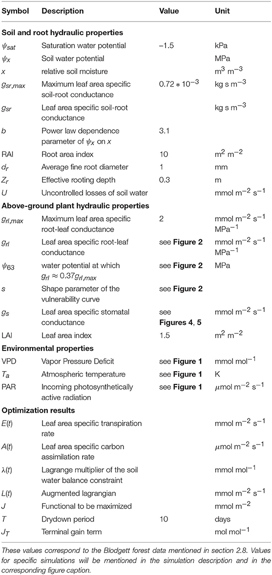
Table 1. Symbols of soil, plant, and environmental properties along with their description, values, and units.

2.5. Leaf-Level Water Balance

As a point of departure from previous analyses based on carbon gain maximization principles where the control variable is g_s, it is recognized that plant transpiration must be limited by soil-plant hydraulics when atmospheric water demand exceeds the potential supply of water from the soil pores. This limitation imposes an upper bound on g_s.

An effective vulnerability to embolism curve (VC) describes the loss of conductivity of the whole plant system with decreasing water potential. For simplicity, the VC of the entire hydraulic pathway (roots, trunk, branches, and leaves) is prescribed with a generic Weibull exceedance function (Sperry and Love, 2015):

$\begin{array}{ll}{g}_{rl}=g_{rl,max}exp[-(\frac{\psi }{{\psi }_{63}}{)}^s],& (12)\end{array}$

where g_rl is the root to leaf hydraulic conductance in mmol m⁻² MPa⁻¹ s⁻¹ expressed per unit leaf area, and g_rl,max is its maximum value at saturation. The ψ₆₃ is the water potential at which the plant loses about 63% of its conductance, as common in Weibull VCs. Finally, s dictates the shape and curvature of the Weibull function. The E at the soil, plant, and leaf levels must satisfy the continuity equation at steady-state:

$\begin{array}{l}E=E_{demand}=1.6g_s\text{VPD}\\ =E_{sr}=g_{sr}({\psi }_x)({\psi }_x-{\psi }_r)\\ =E_{rl}={\displaystyle {\int }_{{\psi }_l}^{{\psi }_r}}{g}_{rl}(\psi )d\psi .& (13)\end{array}$

Here, E_demand is the atmospheric demand of water, E_sr is the soil to root water supply, E_rl is the root to leaf supply. All expressions of E are given in units of mmol m⁻² s⁻¹ expressed per unit leaf area. The E_rl expression is analogous to porous media methods where it is recognized that water potential is not distributed hydrostatically along the medium.

It is noted that as g_s varies with time, ψ_l also varies in time to match supply and demand. The hydraulic constraint from the plant water supply system is apparent when one realizes that while E_demand undergoes a limitless increase with rising g_s, water supply through E_sr and E_rl have maxima that cannot be exceeded due to concomitant decreases in hydraulic conductance functions g_sr and g_rl with increasing ψ_x, ψ_r, and ψ_l (Equations 11, 12, and 13). The presence of a maximum possible water supply imposes an additional constraint on the stomatal conductance g_s.

The E_rl expression in Equation (13) only asymptotically reaches a maximum. So, for computational reasons, a critical transpiration rate E_crit is now introduced to define a maximum possible water supply. The E_crit is defined at the ψ_l where the in-series combination of soil-root g_sr and root-leaf conductance is 5% of its maximum values (Sperry et al., 2017). One finds this combined conductance by computing the partial derivative of E with respect to ψ_l such that the condition becomes (see Appendix 2 for detailed derivations):

$\begin{array}{ll}\frac{\partial E}{\partial {\psi }_l}({\psi }_l)=0.05\frac{\partial E}{\partial {\psi }_l}({\psi }_x),& (14)\end{array}$

where it is recognized that the maximum conductance of the whole water pathway at a certain x will occur when all water potentials are in equilibrium with ψ_x due to the monotonically increasing nature of g_sr and g_rl (Equations 11, 12). At this condition, the critical leaf water potential ψ_{l, crit} is attained as well as the corresponding critical root water potential ψ_{r, crit} all being in equilibrium at E = E_crit.

What is sought after is how g_s is constrained by this maximum transpiration rate. One option would be to use an additional Lagrange multiplier to impose this constraint. Although mathematically neater, such a practice will lead to λ in Equation (1) losing its traditional definition of marginal water use efficiency. To avoid this, the maximum transpiration rate constraint is imposed in the following manner: If maximizing J_WUS (Equation 3) leads to a g_s that exceeds the maximum achievable E (E_crit) at current x, this g_s is replaced by its value when E = E_crit to ensure that Equation (14) is satisfied. Here, the assumption that plants take full advantage of their maximum transpiration capacity only applies to those intervals when E exceeds E_crit and is therefore forcibly set to its value at current x.

2.6. Maximizing the Objective

From the definition of J_WUS (Equation 3), there are 5 independent variables: g_s, x, dx/dt, λ, and t. To maximize J_WUS, the calculus of variations (Witelski and Bowen, 2015) is used to derive what are known as the Euler-Lagrange equations (Appendix 1; see Equation 3.55 in the mentioned reference). For this problem, these are a set of three equations to be simultaneously solved with two boundary conditions set on x at the beginning of drydown (x(0) at t = 0) and on λ at the end of the drydown period (λ(T) at t = T). Solving these equations will yield the trends of the 5 independent variables with time so as to maximize J over the mean inter-pulse period T.

The use of this method leads to the so-called control equation,

$\begin{array}{ll}\frac{\partial L}{\partial g_s}=\frac{\partial A}{\partial g_s}+\lambda \frac{\partial f_e}{\partial g_s}=0,& (15)\end{array}$

which gives a monotonic inverse relation between λ and g_s (see section 3). One views Equation (15) as a control equation because the derivative of L with respect to g_s is being evaluated and g_s “controls” the rate of soil water loss through transpiration.

The co-state equation is $\frac{\partial L}{\partial x}-\frac{d}{dt}\left(\frac{\partial L}{\partial x^{\prime }}\right)=0$, where $x^{\prime }=\frac{dx}{dt}$ is used for notational consistency with Witelski and Bowen (2015). The co-state equation yields the time variation of λ:

$\begin{array}{ll}\frac{d\lambda }{dt}=-\frac{\partial A}{\partial x}+\lambda \frac{\partial f_e}{\partial x}=\lambda \frac{\nu }{n{Z}_r}\frac{\partial U}{\partial x},& (16)\end{array}$

where ∂A/∂x = 0 because A only depends on g_s, which is an independent variable itself (∂g_s/∂x = 0).

Finally, the state equation, $\frac{\partial L}{\partial \lambda }=0$ provides the soil water balance (Equation 8). It is to be noted that if x does not vary appreciably in time or varies on time scales much longer than g_s, ∂U/∂x = 0 and dλ/dt = 0 or, simply put, λ = constant. This simplification for x recovers the original arguments put forth by Cowan, Givnish, Farquhar, Hari and recent extensions (Cowan and Farquhar, 1977; Hari et al., 1986; Konrad et al., 2008; Katul et al., 2010; Medlyn et al., 2011).

Another major departure from prior optimization studies are the boundary conditions. Equations (8, 15, 16) are to be solved with preset initial and terminal soil moisture as noted before:

$\begin{array}{l}B{C}_1:x(0)\\ B{C}_2:\lambda (T)=\Lambda .& (17)\end{array}$

A large Λ allows mathematically setting a conservative WUS. Conversely, setting Λ to a small value allows mathematically setting an aggressive WUS for the plant. This approach departs from the assumption that carbon gain trends are instantaneously optimal for all plants because residual soil moisture at the end of dry-down now has a “carbon value” set by Λ. The presence of J_T in Equation (3) represents an opportunity cost, measured in carbon gain units, of depleting the soil of water and increasing cavitation on the short term. The emergence of the boundary conditions in Equation (17) are due to the specific J_T expression in Equations (4). In fact, J_T can take other forms that alter the boundary conditions shown above. For example, J_T could be bigger for situations where refilling is minimal and the replacement of the damaged sapwood to recover lost conductance could provide the carbon cost of embolism. These alternate forms are to be treated in future work.

This description can discern the simultaneous effects of long-term WUS and concomitant VCs as well as sub-daily fluctuations in environmental drivers on optimal trajectories of stomatal behavior g_s(t). Also, because λ here purposely maintains its conventional form of marginal water use efficiency, starting from a specified x(0), the diurnal evolution of λ can be predicted in a manner consistent with the long-term WUS imposed by the conditions λ(T) = Λ. A number of experiments reported variability in measured λ = (∂A/∂g_s)/(∂E_demand/∂g_s) during the course of a day and argued that such variability is evidence against optimal stomatal functioning (Fites and Teskey, 1988). The dynamic optimality approach proposed here makes it clear that optimal stomatal functioning and short-term (sub-hourly) variability in λ are expected and such variability in λ does not preclude optimal stomatal behavior.

2.7. The Gain-Risk or Profit Maximization Approach

This section presents the gain-risk or profit maximization approach (Sperry and Love, 2015; Sperry et al., 2016). This approach will only be used as a comparison to the currently proposed model. Under the profit maximization approach, the so-called profit term to be maximized is defined in terms of a relative gain β (Sperry et al., 2017):

$\begin{array}{ll}\beta =\frac{A({\psi }_l)}{A_{max}({\psi }_x)},& (18)\end{array}$

and a relative loss θ:

$\begin{array}{ll}\theta =\frac{g_{max}({\psi }_x)-g({\psi }_l)}{g_{max}({\psi }_x)-g_{crit}({\psi }_x)}.& (19)\end{array}$

where A is, as before, the instantaneous assimilation rate and depends on both ψ_x and ψ_l, and A_max is here defined as the carbon assimilation rate when E = E_crit. g_max is defined at ψ_l = ψ_x and is the maximum conductance from soil to leaf at a particular ψ_x. The g_crit is here defined as above (= 0.05g_max). Profit is then written as:

$\begin{array}{ll}\text{profit}=\beta -\theta .& (20)\end{array}$

It is now assumed that plants instantaneously maximize the profit by freely varying ψ_l. To analytically impose this condition, the partial derivative of the profit is set to zero to obtain:

$\begin{array}{ll}\frac{\partial \beta }{\partial {\psi }_l}=\frac{\partial \theta }{\partial {\psi }_l}& (21)\end{array}$

and must be satisfied at every instant.

2.8. Environmental Data, Plant Species and Property Selection

The model requires diurnal variations of the environmental variables including VPD, PAR, T_a, and c_a. The measurements provided by the FLUXNET2015 dataset (DOI: 10.18140/FLX/1440068) at Blodgett forest are used as a case study as this forest is known to experience episodic droughts. A dry-down period starting on May 29, 2004, was chosen and the environmental variations over 100 days are binned into one ensemble of diurnal variations. These diurnal conditions are then repeated and tiled to all days defining the period T (Figure 1). This repeating pattern of diurnal environmental conditions allows isolating plant hydraulics and WUS from day-to-day variations in environmental drivers. This particular choice was made because of the need to specify values to model parameters. Any other dataset, in another biome that is mainly water stressed, could be used by altering the parameter values described in this text and in Table 1. The most abundant species at the Blodgett site is Pinus ponderosa. This species will be used to parameterize the photosynthetic variables for this test case. Temperature response curves for V_c,max and J_max of Pinus pinaster from Medlyn et al. (2002) were used. The V_c,max and J_max at 25°C correspond to the ones reported at Blodgett forest for Pinus ponderosa (Panek, 2004). This test case is used to explore general trends of the effects of competition and hydraulic limitations of g_s and ψ_l. Three “canonical” VCs are compared throughout the study and they represent a steep and resistant VC with ψ₆₃ = −4.3 MPa, s = 5.4, and g_rl,max = 2 mmol m⁻² MPa⁻¹ s⁻¹, a steep and vulnerable VC with ψ₆₃ = −1.5 MPa, s = 5.4, and g_rl,max = 2 mmol m⁻² MPa⁻¹ s⁻¹, and a gradual and resistant VC with ψ₆₃ = −4.3 MPa, s = 2, and g_rl,max = 2 mmol m⁻² MPa⁻¹ s⁻¹. These are plotted in Figure 2. These VCs were chosen such that the steep and resistant VC corresponds to that reported in Hubbard et al. (2001) for Pinus ponderosa. The gradual and resistant VC (an exponential shaped VC) is closest to what one would expect of a Quecus species (Christman et al., 2012). Although for complete comparison with Quercus, one would also need to change the photosynthetic parameters as well as those related to the root system. The “plants” to which these VCs pertain are now termed “model plants.” Therefore, while photosynthetic parameters correspond to Pinus ponderosa, VCs were varied to cover a spectrum of hydraulic parameters of interest. T is selected to be on the order of 10 days and the starting soil moisture is low for this case simulation. This is to highlight the transition from demand driven transpiration to supply limited. Environmental variables are averaged over 0.5 h time scales.

FIGURE 1

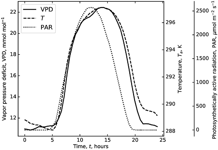
Figure 1. Diurnal trends of vapor pressure deficit (VPD), temperature (T), and photosynthetically active radiation (PAR). These are the averaged trends using measurements from the FLUXNET project at the Blodgett forest over 100 days starting from 5-29-2004 (the start of a 4-month drought). These trends are repeated for the desired simulation duration.

FIGURE 2

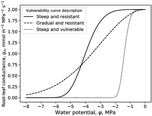
Figure 2. Loss of conductance curves for the three plants simulated throughout this work. The steep and resistant vulnerability curve has parameters ψ₆₃ = −4.3 MPa, s = 5.4, and g_rl,max = 2 mmol m⁻² MPa⁻¹ s⁻¹, the gradual and resistant has ψ₆₃ = −4.3 MPa, s = 2, and g_rl,max = 2 mmol m⁻² MPa⁻¹ s⁻¹, and the steep and vulnerable has ψ₆₃ = −1.5 MPa, s = 5.4, and g_rl,max = 2 mmol m⁻² MPa⁻¹ s⁻¹.

The study proceeds to a second case to compare model results with experimental data conducted elsewhere (Venturas et al., 2018). This was a controlled experiment with aspen saplings undergoing four different treatments. The comparison, discussed later in more detail, is concerned with the “severe drought” treatment in the mentioned study. The model parameterization for this comparison is different than that shown in Table 1. The atmospheric variables for this comparison were those measured during the experiment and available in the aforementioned publication. The vulnerability curve used was that of aspen: ψ₆₃ = −3.6 MPa, s = 1.6, and g_rl,max = 27 mmol m⁻² MPa⁻¹ s⁻¹ per unit leaf area. The LAI is 0.15, the average value for the “severe drought” experiment in Venturas et al. (2018). V_c,max = 120 μmol m⁻² s⁻¹ and j_max = 160 μmol m⁻² s⁻¹ at a leaf temperature of 25 degrees celsius. Z_r = 0.8 m, n = 0.42 for sandy clay loam soil (Clapp and Hornberger, 1978), soil parameters ψ_{x, sat} = 2.8 kPa, $g_{sr,max}=0.12\times 10^{-3}$ kg s m⁻³, and b = 4 for the same soil type (Campbell and Norman, 2012). The simulation was run for 87 days: the length of the “severe drought” treatment (Venturas et al., 2018).

Both cases neglect high-frequency changes in environmental variables (e.g., those commensurate to turbulent time scales that may range from fractions of seconds to minutes) as well as those occurring over monthly and longer times scales such as changes in leaf nitrogen, RAI, LAI, or adjustments in VCs (e.g. due to membrane fatigue). Both cases also neglect soil evaporation in the formulation of U. Gardner (1959) has long shown that the rate of soil evaporation decreases with the square root of time, meaning that the longer the drought, the less soil evaporation is important as a cumulative effect. This is not to say that this cumulative effect is not at all important, but that for long droughts this approximation is more plausible. More accurate use of the calculus of variations framework might include soil evaporation losses in U.

Before presenting the results of this work, it is helpful to summarize the definition of some terms for the sake of clarity and precision. The WUS lies on a spectrum varying from aggressive to conservative water use. It is used in comparative terms among two or more plants. For the same hydraulic, allometric, and photosynthetic traits, an aggressive water user exhibits a higher transpiration rate at the same x compared to a more conservative user. WUS is tightly connected to parameter Λ introduced in Equation (4). Λ imposes a value on the marginal water use efficiency at the end of dry-down λ(T) as discussed above. This is how the ecologically significant and experimentally measurable term λ, known as the marginal water use efficiency, is related to this work's definition of WUS. WUS is a prescribed property of the modeled vegetation. The concept of aniso-/iso-hydry relates to the control of g_s with drying soil. It is also a comparative descriptor used to contrast stomatal response to drought in two or more plants. In this work, a plant is considered to be anisohydric relative to other plants if it exhibits a more rapid decrease in g_s with a marginal decrease in degree of soil saturation x. This control of g_s also translates into a corresponding ψ_l behavior with drying soil as a result of mass conservation (Equation 13). An isohydric species better maintains this control of ψ_l with drying soil compared to an anisohydric species that could see a more rapid decline in ψ_l. Essentially, in this article, no stomatal behavior is labeled as merely isohydric, for example, but it is called isohydric only compared to another plant's drought behavior. This is consistent with the spectrum approach of plant drought tolerance and behavior (Martínez-Vilalta et al., 2014; Garcia-Forner et al., 2016). It is imperative to highlight the fact that iso-/aniso-hydry is an emergent property of the optimization and is not prescribed. It arises from the prescribed WUS and the optimal trajectories of g_s and ψ_l over period T for the gains, costs, and constraints in the Euler-Lagrange equations described above.

3. Results

3.1. Supply Limited Transpiration

Replacing Equations (7) and (8) into Equation (15) provides a functional dependence between g_s, λ, and environmental variables (Katul et al., 2010):

$\begin{array}{l}{g}_s=\frac{k_1(c_a-k_2-2{\Gamma }^{*})}{{(k_2+c_a)}^2}+(k_2+c_a\\ -2a\text{ VPD}\lambda )k_1\frac{\sqrt{a\text{ VPD}\lambda (c_a-{\Gamma }^{*})(k_2+{\Gamma }^{*})(k_2+c_a-a\text{ VPD}\lambda )}}{a\text{ VPD}\lambda {(k_2+c_a)}^2(k_2+c_a-a\text{ VPD}\lambda )},& (22)\end{array}$

where g_s is defined per leaf area as before. The most hydraulically influential atmospheric variable is VPD as it sets the upper boundary condition on the movement of water. In the case where water supply is not limited by the rhizosphere or the plant water pathway (Equations 11, 12), g_s decreases as the air dries (and VPD increases) and vice versa for constant λ. Moreover, as λ increases, g_s decreases. Equation (22) is not bound from above in that if λ is constant, as is the case when no uncontrolled losses exist (Equation 16), a rise in VPD will lead to an unimpeded, albeit decelerating, rise in E. At some point, this rise in g_sVPD will lead to a demand driven E that exceeds the critical value E_crit. At this point, it would be necessary to limit E = E_crit which involves changing the value of λ to achieve this equality. This is where supply limited transpiration “kicks in.”

Supply limited transpiration occurs when the plant water pathway is inhibited enough by cavitation or when the soil is dry enough to set upper limits on E (West et al., 2008). This upper limit is labeled E_crit and defines the maximum allowable transpiration rate. Critical values of g_rl, g_sr, ψ_r, and ψ_l at different ψ_x are shown in Figures 3B,C. Figure 3A shows the partitioning of the total soil-root-leaf conductance into its soil-root and root-leaf components.

FIGURE 3

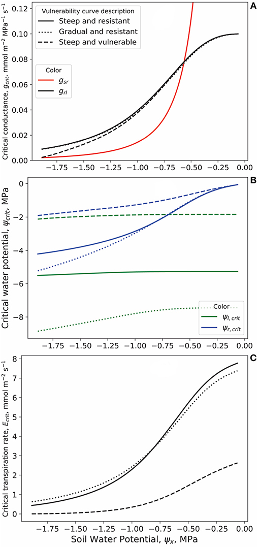
Figure 3. (A) Soil to root conductance of the rhizosphere (g_sr) and root to leaf conductance of the plant (g_rl) at the critical transpiration rate E_crit for different soil water potentials ψ_x. Soil is sandy loam and particular hydraulic parameters are shown in Table 1. Three vulnerability curve (VC) examples give different g_rl trends. The VCs are described and plotted in Figure 2. (B) Critical root and leaf water potentials (ψ_{r, crit} and ψ_{l, crit}, respectively) for the three VCs and for the particular soil type. The gradual and resistant VC (s = 2) can maintain a gap between ψ_r and ψ_l as ψ_x decreases unlike the other two VCs. (C) The critical transpiration rates E_crit for the three VCs. Details on how these curves were derived are available in the main text.

Because the g_sr and g_rl are in series, the total conductance from soil to leaf is limited by the lowest of the two. Therefore, the crossover point between g_sr and g_rl is a dynamically interesting point. Soil water conductance g_x depends on ψ_x (Equation 9) with the exponent 2b + 3 having a value of 9.1 for sandy loam (Campbell and Norman, 2012). This makes water movement from the soil to the roots a limiting factor at low soil moisture values. The crossover point occurs at the same ψ_x for all three VCs (at ≈ –0.6 MPa). The location of this crossover point along the ψ_x axis is dependent on soil type and would occur at higher ψ_x (less negative) for more porous soil because of the stronger ensuing dependence of g_x on ψ_x. Moreover, this crossover point weakly depends on the definition of E_crit: here E_crit is set at the point where the total water conductance is 5% its maximum value. If the definition to limit E is changed to the point of 10% conductance, then that crossover point would switch from ≈ –0.6 MPa to ≈ –0.45 MPa (not shown).

At drier soil, g_sr becomes more limiting than g_rl and becomes the “bottleneck” to the water supply to the leaves. Both the steep model plant VCs experience a reduction in the ψ_r − ψ_l difference as ψ_x decreases to more negative values. A marginally larger ψ_r − ψ_l difference would lead to a negligible increase in water conductance of the entire hydraulic pathway (Figure 3B). In contrast, this trend is absent for the plant with a gradual VC because it can sustain lower ψ_l without catastrophic loss of g_rl (Figure 2). Signs that plant hydraulics drive relative iso- and aniso-hydric behavior are becoming apparent already at this stage. When transpiration is supply limited, ψ_{l, crit} still decreases with ψ_x for a gradual VC (smaller parameter s magnitude) such as in relatively anisohydric plants compared to the more isohydric behavior of the steeper VCs where Figure 3 shows an almost constant ψ_{l, crit} with ever decreasing ψ_x.

3.2. Sensitivity of Stomatal Conductance to Drying Soil

The three VCs mentioned earlier are now compared by modeling a dry-down under two cases: with competition and without competition with other similar plants. In all model runs, WUS was predefined such that the three model plants seek the same target λ(T). This specification is equivalent to maximizing J_WUS of Equation (4) that includes a finite terminal gain J_T. Examples of J maximization (Equation 2) in the absence of J_T were studied in detail elsewhere (Manzoni et al., 2013) and are not repeated here. The cases, selected purposely, reflect the following: if the three plants start their uptake from the same x(0) and end at the same x(T), the vulnerable plant would have to adopt a more aggressive WUS than the other two. This is due to the more limiting VC of the vulnerable plant (Figure 2) that leads to less realistic results. It is expected that more resistant plants to be at least as aggressive as more vulnerable ones if competing for the same water. This expectation is based on the plausible assumption that a more hydraulically resistant plant will push soil moisture levels lower to gain a competitive advantage against more vulnerable plants. This expectation forms the argument as to why J_WUS, instead of merely J, was maximized.

Figure 4 compares the three VCs under a small section of a drought where transpiration transitions from demand to supply limited. The selected period is T = 10 days without competition. All plants commence at the same x(0) = 0.25 (i.e., after some initial phase where drainage and soil evaporation reduced x) and target the same λ(T) = 1.6 mmol mol⁻¹. The vulnerable plant only achieved x(T) = 0.169 compared to the steep and resistant plant's x(T) = 0.152 and a x(T) = 0.147 for the gradual VC at the end of dry-down. Figure 4A sheds light on this difference when g_s is tracked. An earlier decline in g_s occurs after 3 days for the vulnerable plant. This g_s decline is mirrored in Figure 4B where λ for the vulnerable plant experiences earlier midday increases. Equation (16) for this model run indicates that no change in λ should occur because of the absence of competitive water sinks and this is the case for the first 4 days. After the four-day period, however, cavitation in the plant hydraulic pathway limits λ from below and therefore g_s from above (Equation 22; as discussed at the beginning of the Results section). This limitation occurs in all three plants eventually within 8 days but earlier for the vulnerable plant. Therefore, a difference in carbon assimilation and transpiration (Figures 4C,D) of cumulative values at the end of dry-down ${\int }_0^{T}A(t)dt=2.55$ mol m⁻² and ${\int }_0^{T}E(t)dt=547$ mol m⁻² for the steep and resistant plant VC, ${\int }_0^{T}A(t)dt=2.62$ mol m⁻² and ${\int }_0^{T}E(t)dt=574$ mol m⁻² for the gradual plant VC, and ${\int }_0^{T}A(t)dt=2.29$ mol m⁻² and ${\int }_0^{T}E(t)dt=447$ mol m⁻² for the vulnerable plant VC is observed. Of ecological interest are Figures 4E,F that show the sensitivity of modeled midday g_s and ψ_l to ψ_x. One concludes that the vulnerable model plant is a relatively isohydric species due to the high sensitivity of g_s (reaching about 12 mmol m⁻² s⁻¹) to ψ_x and the fact that ψ_l of the vulnerable plant stays constant at about –1.9 MPa below ψ_x of –0.25 MPa. These trends are the opposite for the two other model plants over this range, and this would make them appear relatively anisohydric: g_s maintaining a value of 38 mmol m⁻² s⁻¹ even at ψ_x = −0.4 MPa and ψ_l reaching as low as –11 MPa for the gradual model plant. These different trends are of purely hydraulic origins based on VC differences only. For even drier soil conditions (ψ_x < −0.4 MPa) conditions, a shift in behavior is observed for the resistant and exponential plants.

FIGURE 4

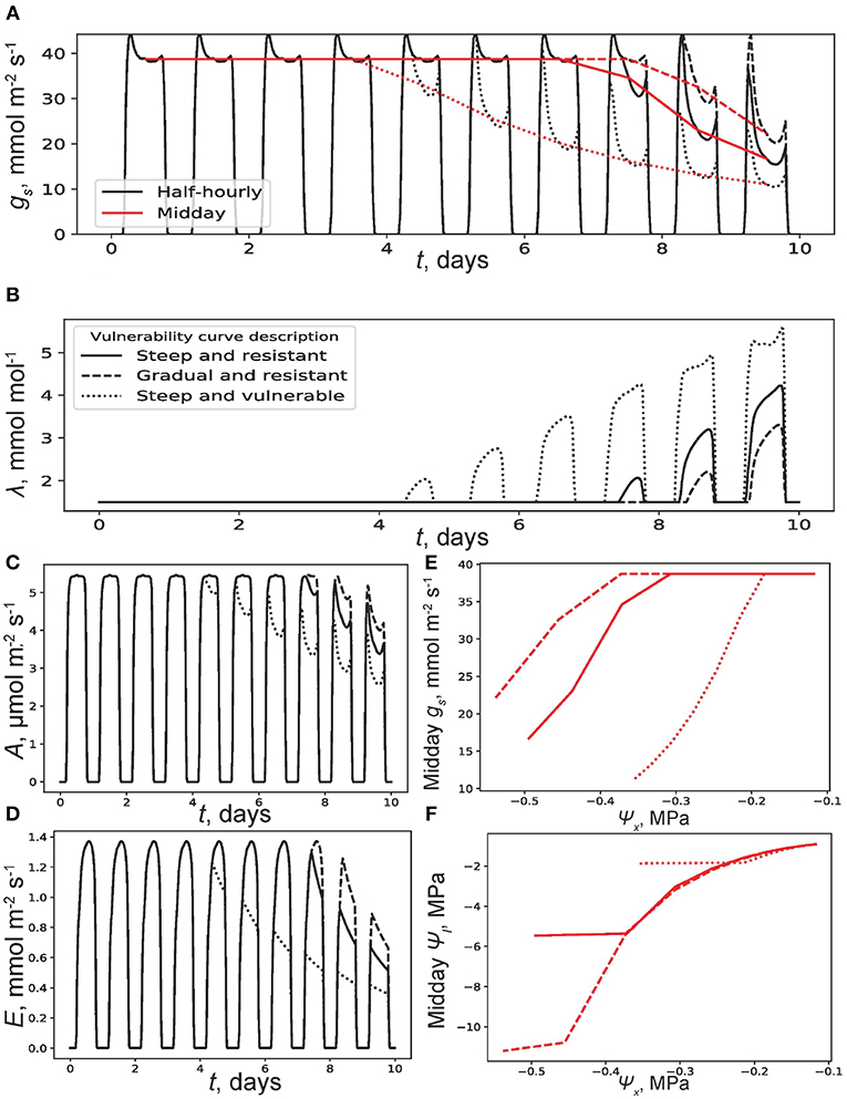
Figure 4. Results of a simulation where at time t = 0, soil moisture x(0) = 0.25. There are no competitive soil water users and the terminal marginal water use efficiency is set at λ(10) = 1.6 mmol mol⁻¹. (A) Half-hourly (black) and midday (red) trends of stomatal conductance (g_s) with t and (B) λ with t. Trends are shown for the three vulnerability curves (VCs) described and plotted in Figure 2. Other plant and soil parameters are listed in the Table 1. (C) Carbon assimilation rate (A) and (D) transpiration rate (E) with t. (E) Midday g_s and (F) midday leaf water potential ψ_l with soil water potential ψ_x.

Equation (16) suggests that one of the many possible reasons for the sensitivity of λ to ψ_x is the presence of uncontrolled competitive water sinks U. To illustrate this phenomenon, U is set to the following:

$\begin{array}{ll}U=\frac{a_{grav}}{M_w\text{LAI}}{g}_x+E_{comp},& (23)\end{array}$

where the first term on the right hand side is the soil leakage and the second term is transpiration by competition from other plants (E_comp) of the same type of those being modeled (same VC; such as in monocultures). The E_comp includes only competitive transpiration from the rooting zone of interest. Because these plants have same VC as the modeled plant and assuming that rooting zone water content is similar for both modeled and competitive plant E_comp is proportional to E. For the purpose of illustrating the effect of competition, E_comp = 0.2E where it is taken that these competitive plants access only 20% of the water in the rooting zone of interest hence the second factor on the right hand side. This number will change depending on tree-to-tree spacing, biome, soil type and other ecosystem specific properties but is given an arbitrary value here for the purpose of running the model. The first factor on the right hand side of Equation (23) contains the acceleration due to gravity a_grav = 9.81 m s⁻² and makes sure all terms have units of mmol m⁻² s⁻¹. This gives the following time derivative of λ (Equation 16; see detailed calculations of terms containing E_comp in Appendix 3):

$\begin{array}{ll}\frac{d\lambda }{dt}=\lambda (t)\frac{\nu }{n{Z}_r}(\frac{a_{grav}}{M_w\text{LAI}}{g}_{x,sat}(2b+3)x^{2b+2}+\frac{\partial E_{comp}}{\partial x}).& (24)\end{array}$

For dry soils such as the one modeled, the first term of Equation (24) would be negligible because of the high exponent raised on x. All terms are positive and therefore always lead to positive dλ/dt or increasing λ with time during dry-down.

This is illustrated in Figure 5. In this model calculation, the target λ(T) for all three species is set to 2.5 mmol mol⁻¹ and x(0) and T were set equal to the previous runs depicted in Figure 4. It is apparent from Figure 5B that all three plants start with a λ(0) < 2.5 mmol mol⁻¹ and experience a steady increase due to competition (Equation 24). Because the vulnerable plant competes with its equally vulnerable peers, it experiences a slower increase in λ compared to the other two plants ($\frac{\partial E_{comp}}{\partial x}$ is smaller; Equation 24). Therefore, λ(0) of the vulnerable plant starts at a higher value compared to the two other plants. This is mirrored by a lower starting g_s for the vulnerable plant (Figure 5A). Compared to the previous model run without competition, there are earlier signs of hydraulic limitation on all plants starting at only the end of the third day for the vulnerable plant (the minor bump in λ in Figure 5B). This is because rooting zone water depletion is accelerated by competition. An x(T) = 0.163 for the vulnerable plant VC, x(T) = 0.142 for the steep and resistant plant VC, and x(T) = 0.135 for the gradual and resistant plant VC emerge. Obviously, the three transpired the same fraction (83.3%) of the used water. Also, ${\int }_0^{T}A(t)dt=2.36$ mol m⁻² and ${\int }_0^{T}E(t)dt=498$ mol m⁻² for the steep and resistant plant VC, ${\int }_0^{T}A(t)dt=2.46$ mol m⁻² and ${\int }_0^{T}E(t)dt=533$ mol m⁻² for the gradual plant VC, and ${\int }_0^{T}A(t)dt=2.11$ mol m⁻² and ${\int }_0^{T}E(t)dt=402$ mol m⁻² for the vulnerable plant. All cumulative E and A values are lower in this model run compared to their counterparts in the previous model runs due to competition. Although there is a significant difference in the sensitivity of g_s to ψ_x in this model run compared to the last, the trends of ψ_l vs ψ_x are strikingly similar (Figures 5E,F). Figure S1 shows a time extension of 60 days total for this simulation (i.e. with root competition) for the gradual and resistant model plant VC. This is to highlight the ability of this scheme to represent time scales more aligned with extended droughts.

FIGURE 5

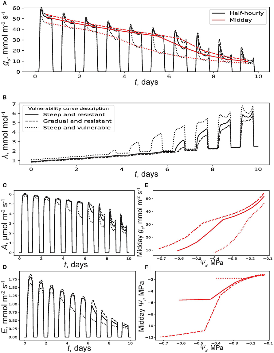
Figure 5. Results of a simulation where at time t = 0, soil moisture x(0) = 0.25. The terminal marginal water use efficiency is set at λ(10) = 2.5 mmol mol⁻¹. The competitive water sinks are soil free drainage and competing plants with similar vulnerability curves (VCs) and water use strategy (WUS) to those modeled. The competing plants have access to only 20% of the root zone water of each modeled plant. (A) Half-hourly (black) and midday (red) trends of stomatal conductance (g_s) with t and (B) λ with t. Trends are shown for the three vulnerability curves (VCs) described and plotted in Figure 2. Other plant and soil parameters are listed in the Table 1. (C) Carbon assimilation rate (A) and (D) transpiration rate (E) with t. (E) Midday g_s and (F) Midday leaf water potential ψ_l with soil water potential ψ_x.

Figures S2A,B-1 shows the decline in c_i/c_a as the soil dries for both simulations (Figure 4). As hydraulic limitations “kick in,” the lower carbon concentration inside the leaf ensures optimal behavior. This is similar to the experimental findings that c_i/c_a are lower in more arid climates (Prentice et al., 2014) although here the variation takes place over finer time scales compared to the mentioned study. There is high midday soil to leaf percent loss of conductance (PLC) for the three plants (Figure S2A-2; ≈ 100%). This is mainly due to soil to root hydraulic constraints (Figure 3). It is important to note that the PLC values shown in Figure S2 integrate the whole soil to leaf pathway and are not to be compared with the organ level PLCs measured in experimental studies. This high soil to leaf PLC can also be avoided by adding non-stomatal limitations such as mesophyll resistance to CO₂ assimilation (not shown here). Trends in c_i/c_a for the simulations with competition show close resemblance to those of g_s (compare Figure 5, Figure S2B-1). Again, there is high soil to leaf PLC for all three plants at about ψ_x = −0.5 MPa (Figure S2B-2).

3.3. Comparison With a Controlled Experiment

Figure 6 compares model results (in red) to experimental data (in black) presented elsewhere (Venturas et al., 2018). The three trends shown are those for g_s, E, and A as a function of soil water potential ψ_x. The relevant hydraulic properties of the modeled aspen are mentioned in the Methods section. Competition was set to have access to 60% of the modeled rooting zone water. Such a high number is due to the experimental setup, explained in the aforementioned study, where multiple saplings were planted in the same plot. The trends shown in Figure 6 have some scatter because, unlike the simulations discussed before, the atmospheric variables were not averaged. While the g_s trends show agreement throughout the ψ_x axis, the trends in E are overestimated by the model for high ψ_x magnitudes (less negative). Moreover, the trends in A are slightly overestimated throughout the whole ψ_x range. This could be amended by a more accurate description of the temperature dependence of V_c,max and j_max. Another important point is that for such a low LAI canopy, soil evaporation contributes to a non-trivial fraction of soil water loss. In the simulations shown here, for simplicity, these evaporative losses were overlooked and their addition should lead to closer agreement with measured E. One can also achieve better agreement by modeling a multi-layered soil where soil water potential within various soil layers as well as hydraulic redistribution is allowed. In the current simulations, the soil to root conductance severely limits water flow to the leaves but hydraulic redistribution is thought to partly ameliorate this effect (Huang et al., 2017). What is promising is that even with these simplifications, the model does provide good agreement with data. For more complex systems such as the Blodgett forest ecosystem, where understory species are prevalent and roots are deeper, it is necessary to refine the representation of uncontrolled losses U to achieve acceptable agreement. In biomes where the primary stressor is, for example, salt stress or leaf heating, the added constraints are to be formulated in Equation (3) for an accurate description of stomatal response to the environment.

FIGURE 6

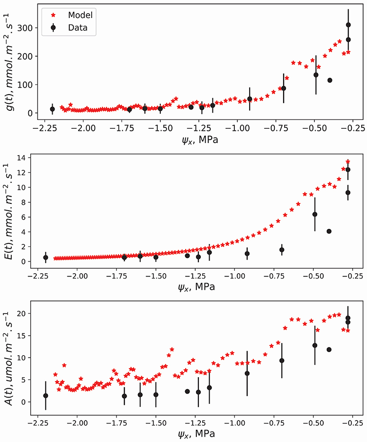
Figure 6. Comparison of model results with the experimental data of Venturas et al. (2018). Top to bottom are the stomatal conductance per leaf area, transpiration rate per leaf area, and the carbon assimilation rate per leaf area. The atmospheric variables were those measured during the experiment and available in the aforementioned publication. The vulnerability curve used was that of aspen: ψ₆₃ = −3.6 MPa, s = 1.6, and g_rl,max = 27 mmol m⁻² MPa⁻¹ s⁻¹ per leaf area. LAI is 0.15, the average value for the severe drought experiment in (Venturas et al., 2018). V_max = 120 μmol m⁻² s⁻¹ and J_max = 160 μmol m⁻² s⁻¹ at a leaf temperature of 25 degrees celsius. The supply limited regime starts at ψ_x = −0.55 MPa. Black vertical lines are the confidence intervals of the measurements computed as $1.96\mathrm{\text{SD}}/\sqrt{n}$ where SD is the standard deviation.

3.4. Comparison With the Gain-Risk Approach

The dynamic optimality approach used throughout this work is now compared to the profit maximization approach in Figure 7. In this figure, a plant with the following VC characteristics: ψ₆₃ = −1.5 MPa, s = 4, and g_rl,max = 2 mmol m⁻² MPa⁻¹ s⁻¹ is used under drying soil (−0.45MPa < ψ_x < −0.15MPa). Morning (Figures 7A,D), midday (Figures 7B,E), and evening (Figures 7C,F) g_s trends with ψ_x are shown. There exists competitive model plants having same VCs as the one of interest in these dynamic optimality and profit maximization simulations. Figures 7A–C show the results of the dynamic optimality approach for different target λ(T) ranging from 9 mmol mol⁻¹ to 11 mmol mol⁻¹ for aggressive WUS to more conservative WUS, respectively, while keeping competition access at 16% (dλ/dt = 0.16(∂E/∂x)ν/(nZ_r)). In contrast, Figures 7D–F keep λ(T) = 10.5 mmol mol⁻¹ while varying competition access from 10 to 20%. The g_s sensitivity to ψ_x is now explored for various WUS. The higher λ(T) is, the smaller the value of g_s throughout the whole ψ_x interval (Figures 7A–C). The more aggressive strategies experience a shift in sensitivity to soil water potential. For example, when λ(T) = 9 mmol mol⁻¹, the slope of the curve becomes steeper with drier soil at about –0.27 MPa. This increased sensitivity is due to hydraulic limitations and occurs at all times of the day. The other, milder sensitivity is purely due to the presence of a competitive rooting sink. The most conservative model plant (λ(T) = 11 mmol mol⁻¹) never reaches hydraulic limitations for the ψ_x range considered. One can also notice a systematic decrease in g_s at midday compared to the morning and evening counterparts, and this is due to its sensitivity to VPD. As expected, more competitive environments (access = 20%) experience earlier hydraulic limitations. Second, it is noted that the gain-risk approach results in an unchanged g_s behavior regardless of the WUS or the strength of competition. Moreover, the sensitivity of g_s to ψ_x in the gain-risk approach is similar in magnitude to that of the dynamic optimality approach only after the onset of hydraulic limitations. It is also observed that no combination of WUS or competition access for the dynamic optimality approach achieves a behavior similar to that of gain-risk. This is true at least for the prescribed plant competition.

FIGURE 7

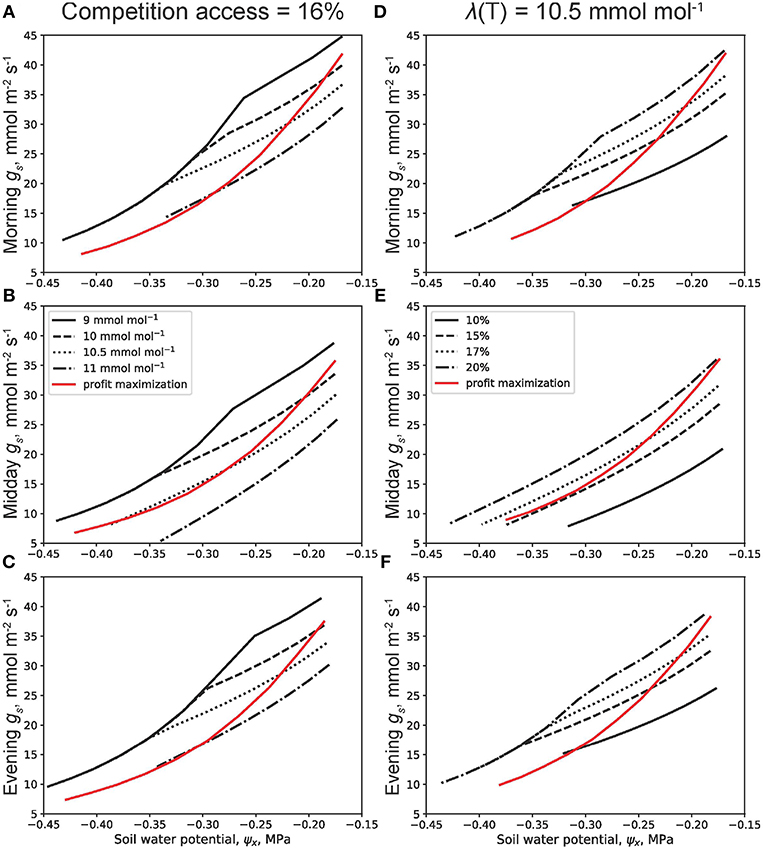
Figure 7. Comparison between the dynamic optimality principle with plant hydraulic constraints and the profit maximization technique. In all panels, the plant is modeled with vulnerability curve (VC) parameters ψ₆₃ = −1.5 MPa, s = 4, and g_rl,max = 2 mmol m⁻² MPa⁻¹ s⁻¹. The plant competes with plants of similar VC and behavior who have access to a certain percentage of the modeled plant's rooting zone water. This percentage is called the competition access percentage. (A–C) vary the terminal marginal water use efficiency λ(T) at the end of drydown t = T while keeping the competition access constant at 16%. (A–C) like (D–F) show the sensitivity of morning, midday, and evening stomatal conductance g_s to soil water potential ψ_x, respectively. (D–F) keep λ(T) = 10.5 mmol mol⁻¹ while varying the competition access.

4. Discussion

The work here extends earlier optimization approaches by adding to the hydrologic balance explicitly as a constraint to be satisfied at every instant. These additions include biotic and abiotic competition for water and variability in environmental drivers that allow the marginal water use efficiency to be described on sub-daily time scales using the co-state equation (Equation 16). The integrated result of the response of g_s to these sub-daily time scale environmental drivers determines the fitness of a plant over a drought period T (see the integral in Equations 2, 3). This integration ensures the compatibility of resolving a sub-daily process (stomatal opening) for the sake of maximizing a multi-day goal (total carbon assimilation). Plant hydraulic limits are imposed as new constraints through VCs using a dynamic optimality approach to g_s (Manzoni et al., 2013). This is an improvement that goes beyond including only soil water balance as a constraint to be satisfied at all times. Moreover, no a priori measurements of the Lagrange multipliers are required because they emerge solely from the solution of the Euler-Lagrange equations (Witelski and Bowen, 2015) provided appropriate boundary conditions can be specified (i.e., partly through water use strategy).

The first optimization approaches to modeling stomatal behavior were developed for conditions where soil moisture does not change appreciably in time, and soil-plant hydraulics do not limit water uptake (Cowan and Farquhar, 1977). In these conditions, the currently proposed approach recovers the conventional optimality solutions for constant marginal water use efficiencies (Katul et al., 2010). Moreover, it is now possible to include a multitude of factors affecting stomatal conductance under drying conditions. The advantage of the dynamic optimality approach lies in the ease with which one adds additional constraints that are pertinent in different environments. One could assess limitations on g_s set by the maintenance of phloem turgor through osmoregulation (Sevanto et al., 2014) or soil salinity for well-watered conditions. Also, additional constraints such as the energy balance can be readily included as has been accomplished in recent studies using a similar framework (Roth-Nebelsick and Konrad, 2018). The inclusion of the additional plant hydraulic constraint was explored in this work but only indirectly using a “hard” threshold on E by maximum water supply E_crit. This addition can be formally treated by introducing an additional Lagrange multiplier thereby offering a smoother transition toward supply limited transpiration.

However, there is evidence that a finite safety margin between E and E_crit and between ψ_l and ψ_{l, crit} exists to avoid E = E_crit (McDowell et al., 2008; Plaut et al., 2012). This shortcoming of the model here can be rectified in the future as discussed later on. This first step, however, is part of recent improvements made with regards to modeling g_s under a drought that quantitatively include the effects of VCs (Sperry and Love, 2015; Sperry et al., 2017). The model results here show emergence of relatively iso- and aniso-hydric responses to drought through the responses of midday g_s and ψ_l to ψ_x (Figures 4, 5). The modeling results show that this behavior also emerges from plants having acclimated to competition for water at the rooting zone. There is no experimental evidence yet on whether this truly occurs though Figure 6 shows good agreement with experiments. Nonetheless, this hypothesis requires further empirical testing.

The model also predicts that during the initial stages of a drought, when transpiration is still demand driven, g_s and E are relatively unchanged in the absence of uncontrolled losses (Figure 4). While this is consistent in the case of E with anisohydric species (Hochberg et al., 2018), in some field experiments g_s shows a significant decline right after the onset of drought (Gollan et al., 1985; Schulze, 1986). This might be driven by changes in VPD as dry spells persist but these are suppressed in the simulations of Figures 4, 5. The proposed model does predict declines in g_s in the presence of competition by other roots even for repetitive daily trends in VPD (Figure 5). Starting from a higher g_s value at drought onset in the presence of plant competition ensures maximal ${\int }_0^{T}Adt$. This is a response to the fact that even if the modeled plant does limit its transpiration for longer term gains, more aggressive water use by competitive agents (biotic or abiotic) could still cause cavitation in its water pathway albeit over a longer period. It is likely, although not captured in the model here, that plants do avoid potential cavitation by pre-emptively reducing E before its critical value E_crit is reached (see Juniperus monosperma in Figure 5B in Garcia-Forner et al., 2016). Adding non-stomatal constraints in the future, such as mesophyll conductance, will buffer rapid declines in c_i (Figures S2A,B-1) and ensure PLC does not reach such high values as shown in Figures S2A,B-2.

The precautionary measure on E is however captured in a recently developed framework (Sperry et al., 2016, 2017) and a comparison with the proposed model here is shown (Figure 7). The aforementioned framework is called the gain-risk approach. It stipulates that leaf economics are governed by the drive to maximize a gain or profit term instantaneously. Profit in that context was introduced as the difference between normalized gain and loss terms (Equations 18, 19). Because these two normalized formulations are expressed in terms of A and soil-leaf conductance, they are purely intrinsic to the plant. Moreover, because external soil water sinks and sources directly affect plant conductance through rhizosphere water potential, the plant does respond to competitive actors albeit indirectly. The gain-risk approach is therefore suitable for larger scale land-atmosphere exchange models due to the computationally inexpensive yet realistic prediction of g_s responses to drought. In the comparison in Figure 7, it is seen that for different competition types and WUS, the profit maximization approach predicts a single plant response while the dynamic optimality approach predicts a broader spectrum of g_s responses (allowed to vary with WUS). As predicted by the proposed model here, g_s increases for more aggressive WUS (smaller λ(T)) and more aggressive competition (larger competition access). For the specified VC (namely, a vulnerable plant with ψ₆₃ = −1.5 MPa, s = 5.4, and g_rl,max = 2 mmol m⁻² MPa⁻¹ s⁻¹), the proposed model can reproduce the response predicted by the profit maximization approach only for a certain WUS, competition type (competitive plant VC) and access, and/or the inclusion of specific non-stomatal limitations (not shown).

To mechanistically disentangle the impacts of plant hydraulic traits (mainly the shape of the VCs) and water use strategies, the work here focused on the stomatal behavior under given meteorological, edaphic, and phenological conditions. Variability in these environmental conditions is also observed to affect stomatal behavior across time and space (Feng et al., 2018; Novick et al., 2019). However, at long time scales, the impact of such biome-specific environmental conditions can be reflected by the WUS possibly as a result of adaptation. For short-time scales such as a drought, the proposed dynamic optimality approach allows exploring stomatal behavior by integrating the aforementioned mechanistic constraints with variations in environmental conditions during a drought. Variability in LAI and RAI as well as rooting depth can be readily accommodated in this proposed approach but are not considered explicitly here. More importantly, the model results here suggest that the stomatal control strategy is influenced by both the plant vulnerability curve and the environment. The iso-anisohyrdy framework has been used to predict plant mortality mechanisms (McDowell et al., 2008), even if recent studies suggest a more complex picture (Meinzer et al., 2014; Martíez-Vilalta and Garcia-Forner, 2017). In support of the model results, it has been shown experimentally that the metrics of iso- and anisohyrdy depend on the environment when comparing plants with similar VCs (Hochberg et al., 2018). Based on the model results here, the more gradual VC (with lower Weibull parameter s = 2) could have an advantage in WUS over the steeper curves (with s = 5.4) in certain situations. This sheds light on the importance of determining the shape parameter s of vulnerability curves when assessing stomatal responses of trees to drought (Compare Weibull shape parameter of Pinus edulis and Juniperus monosperman in Table 3 of Plaut et al., 2012). It is possible that VC shapes and WUS are not independent and co-evolved to maximize fitness for a set of environmental and edaphic conditions, a topic to be explored in the future.

A specific biome dominated by a conifer species (the Blodgett forest) and an experiment featuring an angiosperm tree were chosen here for the sake of providing plausible parameter values for model runs. The approach presented here is general enough to capture the dynamics of multiple different biomes and functional types. One of those are the semi-arid ecosystem where soil evaporation is a significant source of soil water loss at the beginning of a drought and another is a broad-leaf forest with high LAI provided that one upscales leaf photosynthesis to canopy photosynthesis, among others. What's necessary for a complete comparison with complex ecosystem data such as that in the Blodgett forest includes the addition of: (1) radiation balance to determine layer-wise PAR and photosynthesis, (2) multi-layered soil to capture the effects of variable soil pressure and hydraulic redistribution, (3) a complete formulation of uncontrolled losses U and its rate of change with decreasing soil moisture and this includes competitive plants, drainage, and soil evaporation, (4) correct photosynthesis upscaling especially for high LAI canopies where partitioning leaves into sunlit and shaded portions is necessary (Pury and Farquhar, 1997). All these potential additions can be included in the existing optimality framework here.

5. Conclusions

The goal of this work was to propose a mathematical framework that can accommodate multiple constraints and drivers of stomatal behavior. Our model predicted that the stomatal control of leaf water potential is concomitantly influenced by hydraulic traits and the environment. To extend the applicability of the model, the addition of extra constraints will necessitate the introduction of multiple Lagrange multipliers. The value of these Lagrange multipliers need not be determined a priori as shown in this study. On the contrary, the relative magnitude of these Lagrange multipliers will indicate which constraints shape the response of stomatal aperture to soil drying under different environmental conditions. Such an approach has promise in disentangling the topic of iso- and aniso-hydric stomatal responses to drying that lumps a multitude of physiological constraints on sustained water use under varying environmental conditions. Moreover, in a future work, the model will benefit from an improved terminal gain term J_T in Equation (3). Alternate formulations will depend on traits such as stem growth rates and leaf area to sapwood area ratio. Additionally, potential improvements include a full partitioning of hydraulic traits across organs, leaf energy balance, the maintenance of phloem turgor and osmoregulation, and the influence of chemical signaling from a layered rooting system to model the results of the many split-root experiments conducted in the past (Blackman and Davies, 1985; Zhang et al., 1987). This integrative work represents a frontier of understanding global change through ecosystem vegetation dynamics.

Data Availability

The raw data supporting the conclusions of this manuscript will be made available by the authors, without undue reservation, to any qualified researcher. Access to the Python code, data, TeX files, and BIB files is provided through: https://github.com/mradassaad/Frontiers_Mrad_Sevanto_Domec_Liu_Nakad_Katul.

Author Contributions

AM and YL contributed to the modeling effort. AM, GK, and SS designed the direction of this work. AM, SS, J-CD, YL, MN, and GK contributed to the analysis of the results and in drafting the manuscript.

Funding

GK, AM, MN, and J-CD acknowledge support from the U.S. National Science Foundation (NSF-EAR-1344703, NSF-AGS-1644382, and NSF-IOS-1754893). SS was supported by Los Alamos Directed Research and Development Exploratory Research Grant #20160373ER.

Conflict of Interest Statement

The authors declare that the research was conducted in the absence of any commercial or financial relationships that could be construed as a potential conflict of interest.

Acknowledgments

This work used eddy covariance data acquired and shared by the FLUXNET community, including these networks: AmeriFlux, AfriFlux, AsiaFlux, CarboAfrica, CarboEuropeIP, CarboItaly, CarboMont, ChinaFlux, Fluxnet-Canada, GreenGrass, ICOS, KoFlux, LBA, NECC, OzFlux-TERN, TCOS-Siberia, and USCCC. The ERA-Interim reanalysis data are provided by ECMWF and processed by LSCE. The FLUXNET eddy covariance data processing and harmonization was carried out by the European Fluxes Database Cluster, AmeriFlux Management Project, and Fluxdata project of FLUXNET, with the support of CDIAC and ICOS Ecosystem Thematic Center, and the OzFlux, ChinaFlux and AsiaFlux offices.

Supplementary Material

The Supplementary Material for this article can be found online at: https://www.frontiersin.org/articles/10.3389/ffgc.2019.00049/full#supplementary-material

References

Bernacchi, C. J., Singsaas, E. L., Pimentel, C., Portis, A. R. Jr., and Long, S. P. (2001). Improved temperature response functions for models of Rubisco-limited photosynthesis. Plant Cell Environ. 24, 253–259. doi: 10.1111/j.1365-3040.2001.00668.x

CrossRef Full Text | Google Scholar

Betts, R. A., Boucher, O., Collins, M., Cox, P. M., Falloon, P. D., Gedney, N., et al. (2007). Projected increase in continental runoff due to plant responses to increasing carbon dioxide. Nature 448:1037. doi: 10.1038/nature06045

PubMed Abstract | CrossRef Full Text | Google Scholar

Blackman, P., and Davies, W. (1985). Root to shoot communication in maize plants of the effects of soil drying. J. Exp. Bot. 36, 39–48. doi: 10.1093/jxb/36.1.39

CrossRef Full Text | Google Scholar

Brodribb, T. J., Holbrook, N. M., Edwards, E. J., and Gutiérrez, M. V. (2003). Relations between stomatal closure, leaf turgor and xylem vulnerability in eight tropical dry forest trees. Plant Cell Environ. 26, 443–450. doi: 10.1046/j.1365-3040.2003.00975.x

CrossRef Full Text | Google Scholar

Buckley, T. N., Sack, L., and Farquhar, G. D. (2017). Optimal plant water economy. Plant Cell Environ. 40, 881–896. doi: 10.1111/pce.12823

PubMed Abstract | CrossRef Full Text | Google Scholar

Campbell, G. S., and Norman, J. M. (2012). An Introduction to Environmental Biophysics. New York, NY: Springer Science & Business Media.

Google Scholar

Christman, M. A., Sperry, J. S., and Smith, D. D. (2012). Rare pits, large vessels and extreme vulnerability to cavitation in a ring-porous tree species. New Phytol. 193, 713–720. doi: 10.1111/j.1469-8137.2011.03984.x

PubMed Abstract | CrossRef Full Text | Google Scholar

Clapp, R. B., and Hornberger, G. M. (1978). Empirical equations for some soil hydraulic properties. Water Resour. Res. 14, 601–604. doi: 10.1029/WR014i004p00601

CrossRef Full Text | Google Scholar

Collatz, G. J., Ball, J. T., Grivet, C., and Berry, J. A. (1991). Physiological and environmental regulation of stomatal conductance, photosynthesis and transpiration: a model that includes a laminar boundary layer. Agric. For. Meteorol. 54, 107–136. doi: 10.1016/0168-1923(91)90002-8

CrossRef Full Text | Google Scholar

Cowan, I. (1986). “Economics of carbon fixation in higher plants,” in On the Economy of Plant Form and Function: Proceedings of the Sixth Maria Moors Cabot Symposium, Evolutionary Constraints on Primary Productivity, Adaptive Patterns of Energy Capture in Plants, Harvard Forest, August 1983 (Cambridge: Cambridge University Press), 133–170.

Google Scholar

Cowan, I., and Troughton, J. (1971). The relative role of stomata in transpiration and assimilation. Planta 97, 325–336. doi: 10.1007/BF00390212

PubMed Abstract | CrossRef Full Text | Google Scholar

Cowan, I. R. (1978). “Stomatal behaviour and environment,” in Advances in Botanical Research, Vol. 4, eds R. D. Preston and H. W. Woolhouse (Academic Press), 117–228.

Google Scholar

Cowan, I. R., and Farquhar, G. D. (1977). Stomatal function in relation to leaf metabolism and environment. Symp. Soc. Exp. Biol. 31, 471–505.

PubMed Abstract | Google Scholar

Cox, P. M., Betts, R. A., Jones, C. D., Spall, S. A., and Totterdell, I. J. (2000). Acceleration of global warming due to carbon-cycle feedbacks in a coupled climate model. Nature 408:184. doi: 10.1038/35041539

PubMed Abstract | CrossRef Full Text | Google Scholar

Damour, G., Simonneau, T., Cochard, H., and Urban, L. (2010). An overview of models of stomatal conductance at the leaf level. Plant Cell Environ. 33, 1419–1438. doi: 10.1111/j.1365-3040.2010.02181.x

PubMed Abstract | CrossRef Full Text | Google Scholar

Darwin, F. (1898). Ix. observations on stomata. Philos. Trans. R. Soc. Lond. Ser. B 190, 531–621. doi: 10.1098/rstb.1898.0009

CrossRef Full Text | Google Scholar

Dewar, R., Mauranen, A., Mäkelä, A., Hölttä, T., Medlyn, B., and Vesala, T. (2018). New insights into the covariation of stomatal, mesophyll and hydraulic conductances from optimization models incorporating nonstomatal limitations to photosynthesis. New Phytol. 217, 571–585. doi: 10.1111/nph.14848

PubMed Abstract | CrossRef Full Text | Google Scholar

Dewar, R. C. (2010). Maximum entropy production and plant optimization theories. Philos. Trans. R. Soc. B Biol. Sci. 365, 1429–1435. doi: 10.1098/rstb.2009.0293

PubMed Abstract | CrossRef Full Text | Google Scholar

Dubois, J.-J. B., Fiscus, E. L., Booker, F. L., Flowers, M. D., and Reid, C. D. (2007). Optimizing the statistical estimation of the parameters of the farquhar “von caemmerer” berry model of photosynthesis. New Phytol. 176, 402–414. doi: 10.1111/j.1469-8137.2007.02182.x

CrossRef Full Text | Google Scholar

Farquhar, G. D., von Caemmerer, S., and Berry, J. A. (1980). A biochemical model of photosynthetic CO2 assimilation in leaves of C3 species. Planta 149, 78–90. doi: 10.1007/BF00386231

CrossRef Full Text | Google Scholar

Feng, X., Ackerly, D. D., Dawson, T. E., Manzoni, S., McLaughlin, B., Skelton, R. P., et al. (2018). Beyond isohydricity: the role of environmental variability in determining plant drought responses. Plant Cell Environ. 42, 1104–1111. doi: 10.1111/pce.13486

PubMed Abstract | CrossRef Full Text | Google Scholar

Fites, J., and Teskey, R. (1988). Co2 and water vapor exchange of pinus taeda in relation to stomatal behavior: test of an optimization hypothesis. Can. J. For. Res. 18, 150–157. doi: 10.1139/x88-024

CrossRef Full Text | Google Scholar

Franks, P. J., Drake, P. L., and Froend, R. H. (2007). Anisohydric but isohydrodynamic: seasonally constant plant water potential gradient explained by a stomatal control mechanism incorporating variable plant hydraulic conductance. Plant Cell Environ. 30, 19–30. doi: 10.1111/j.1365-3040.2006.01600.x

PubMed Abstract | CrossRef Full Text | Google Scholar

Garcia-Forner, N., Adams, H. D., Sevanto, S., Collins, A. D., Dickman, L. T., Hudson, P. J., et al. (2016). Responses of two semiarid conifer tree species to reduced precipitation and warming reveal new perspectives for stomatal regulation. Plant Cell Environ. 39, 38–49. doi: 10.1111/pce.12588

PubMed Abstract | CrossRef Full Text | Google Scholar

Gardner, W. R. (1959). Solutions of the flow equation for the drying of soils and other porous media 1. Soil Sci. Soc. Am. J. 23, 183–187. doi: 10.2136/sssaj1959.03615995002300030010x

CrossRef Full Text | Google Scholar

Givnish, T. J., and Vermeij, G. J. (1976). Sizes and shapes of liane leaves. Am. Nat. 110, 743–778. doi: 10.1086/283101

CrossRef Full Text | Google Scholar

Gollan, T., Turner, N. C., and Schulze, E. D. (1985). The responses of stomata and leaf gas exchange to vapour pressure deficits and soil water content. Oecologia 65, 356–362. doi: 10.1007/BF00378908

CrossRef Full Text | Google Scholar

Gu, L., Pallardy, S. G., Tu, K., Law, B. E., and Wullschleger, S. D. (2010). Reliable estimation of biochemical parameters from c3 leaf photosynthesis-intercellular carbon dioxide response curves: estimating fvcb model parameters. Plant Cell Environ. 33, 1852–1874. doi: 10.1111/j.1365-3040.2010.02192.x

CrossRef Full Text | Google Scholar

Hari, P., Mäkelä, A., Korpilahti, E., and Holmberg, M. (1986). Optimal control of gas exchange. Tree Physiol. 2, 169–175. doi: 10.1093/treephys/2.1-2-3.169

PubMed Abstract | CrossRef Full Text | Google Scholar

Hetherington, A. M., and Woodward, F. I. (2003). The role of stomata in sensing and driving environmental change. Nature 424:901. doi: 10.1038/nature01843

PubMed Abstract | CrossRef Full Text | Google Scholar

Hochberg, U., Rockwell, F. E., Holbrook, N. M., and Cochard, H. (2018). Iso/anisohydry: a plant-environment interaction rather than a simple hydraulic trait. Trends Plant Sci. 23, 112–120. doi: 10.1016/j.tplants.2017.11.002

PubMed Abstract | CrossRef Full Text | Google Scholar

Huang, C.-W., Domec, J.-C., Palmroth, S., Pockman, W. T., Litvak, M. E., and Katul, G. G. (2018). Transport in a coordinated soil-root-xylem-phloem leaf system. Adv. Water Resour. 119, 1–16. doi: 10.1016/j.advwatres.2018.06.002

CrossRef Full Text | Google Scholar

Huang, C.-W., Domec, J.-C., Ward, E. J., Duman, T., Manoli, G., Parolari, A. J., et al. (2017). The effect of plant water storage on water fluxes within the coupled soil–plant system. New Phytol. 213, 1093–1106. doi: 10.1111/nph.14273

PubMed Abstract | CrossRef Full Text | Google Scholar

Hubbard, R. M., Ryan, M., Stiller, V., and Sperry, J. (2001). Stomatal conductance and photosynthesis vary linearly with plant hydraulic conductance in ponderosa pine. Plant Cell Environ. 24, 113–121. doi: 10.1046/j.1365-3040.2001.00660.x

CrossRef Full Text | Google Scholar

Jarvis, P. (1976). The interpretation of the variations in leaf water potential and stomatal conductance found in canopies in the field. Philos. Trans. R. Soc. Lond. B Biol. Sci. 273, 593–610. doi: 10.1098/rstb.1976.0035

CrossRef Full Text | Google Scholar

Javelle, P., Fouchier, C., Arnaud, P., and Lavabre, J. (2010). Flash flood warning at ungauged locations using radar rainfall and antecedent soil moisture estimations. J. Hydrol. 394, 267–274. doi: 10.1016/j.jhydrol.2010.03.032

CrossRef Full Text | Google Scholar

Jensen, K. H., Berg-Sørensen, K., Bruus, H., Holbrook, N. M., Liesche, J., Schulz, A., et al. (2016). Sap flow and sugar transport in plants. Rev. Mod. Phys. 88:035007. doi: 10.1103/RevModPhys.88.035007

CrossRef Full Text | Google Scholar

Katul, G., Manzoni, S., Palmroth, S., and Oren, R. (2010). A stomatal optimization theory to describe the effects of atmospheric CO2 on leaf photosynthesis and transpiration. Ann. Bot. 105, 431–442. doi: 10.1093/aob/mcp292

PubMed Abstract | CrossRef Full Text | Google Scholar

Katul, G. G., Oren, R., Manzoni, S., Higgins, C., and Parlange, M. B. (2012). Evapotranspiration: a process driving mass transport and energy exchange in the soil-plant-atmosphere-climate system. Rev. Geophys. 50:RG3002. doi: 10.1029/2011RG000366

CrossRef Full Text | Google Scholar

Katul, G. G., Palmroth, S., and Oren, R. A. M. (2009). Leaf stomatal responses to vapour pressure deficit under current and CO2-enriched atmosphere explained by the economics of gas exchange. Plant Cell Environ. 32, 968–979. doi: 10.1111/j.1365-3040.2009.01977.x

CrossRef Full Text | Google Scholar

Konrad, W., Katul, G., Roth-Nebelsick, A., and Jensen, K. H. (2018). Xylem functioning, dysfunction and repair: a physical perspective and implications for phloem transport. Tree Physiol. 39, 243–261. doi: 10.1093/treephys/tpy097

PubMed Abstract | CrossRef Full Text | Google Scholar

Konrad, W., Roth-Nebelsick, A., and Grein, M. (2008). Modelling of stomatal density response to atmospheric co2. J. Theor. Biol. 253, 638–658. doi: 10.1016/j.jtbi.2008.03.032

PubMed Abstract | CrossRef Full Text | Google Scholar

Leuning, R. (1995). A critical appraisal of a combined stomatal-photosynthesis model for C3 plants. Plant Cell Environ. 18, 339–355. doi: 10.1111/j.1365-3040.1995.tb00370.x

CrossRef Full Text | Google Scholar

Lu, Y., Duursma, R. A., and Medlyn, B. E. (2016). Optimal stomatal behaviour under stochastic rainfall. J. Theor. Biol. 394, 160–171. doi: 10.1016/j.jtbi.2016.01.003

PubMed Abstract | CrossRef Full Text | Google Scholar

Mäkelä, A., Berninger, F., and Hari, P. (1996). Optimal control of gas exchange during drought: theoretical analysis. Ann. Bot. 77, 461–468. doi: 10.1006/anbo.1996.0056

CrossRef Full Text | Google Scholar

Mäkelä, A., and Hari, P. (1986). Stand growth model based on carbon uptake and allocation in individual trees. Ecol. Model. 33, 205–229. doi: 10.1016/0304-3800(86)90041-4

CrossRef Full Text | Google Scholar

Manoli, G., Domec, J.-C., Novick, K., Oishi, A. C., Noormets, A., Marani, M., et al. (2016). Soil–plant–atmosphere conditions regulating convective cloud formation above southeastern us pine plantations. Global Change Biol. 22, 2238–2254. doi: 10.1111/gcb.13221

PubMed Abstract | CrossRef Full Text | Google Scholar

Manzoni, S., Vico, G., Katul, G., Fay, P. A., Polley, W., Palmroth, S., et al. (2011). Optimizing stomatal conductance for maximum carbon gain under water stress: a meta-analysis across plant functional types and climates. Funct. Ecol. 25, 456–467. doi: 10.1111/j.1365-2435.2010.01822.x

CrossRef Full Text | Google Scholar

Manzoni, S., Vico, G., Palmroth, S., Porporato, A., and Katul, G. (2013). Optimization of stomatal conductance for maximum carbon gain under dynamic soil moisture. Adv. Water Resour. 62, 90–105. doi: 10.1016/j.advwatres.2013.09.020

CrossRef Full Text | Google Scholar

Martínez-Vilalta, J., and Garcia-Forner, N. (2017). Water potential regulation, stomatal behaviour and hydraulic transport under drought: deconstructing the iso/anisohydric concept. Plant Cell Environ. 40, 962–976. doi: 10.1111/pce.12846

PubMed Abstract | CrossRef Full Text | Google Scholar

Martínez-Vilalta, J., Poyatos, R., Aguadé, D., Retana, J., and Mencuccini, M. (2014). A new look at water transport regulation in plants. New Phytol. 204, 105–115. doi: 10.1111/nph.12912

PubMed Abstract | CrossRef Full Text | Google Scholar

McDowell, N., Pockman, W. T., Allen, C. D., Breshears, D. D., Cobb, N., Kolb, T., et al. (2008). Mechanisms of plant survival and mortality during drought: why do some plants survive while others succumb to drought? New Phytol. 178, 719–739. doi: 10.1111/j.1469-8137.2008.02436.x

PubMed Abstract | CrossRef Full Text | Google Scholar

Medlyn, B. E., Dreyer, E., Ellsworth, D., Forstreuter, M., Harley, P. C., Kirschbaum, M. U. F., et al. (2002). Temperature response of parameters of a biochemically based model of photosynthesis. II. A review of experimental data. Plant Cell Environ. 25, 1167–1179. doi: 10.1046/j.1365-3040.2002.00891.x

CrossRef Full Text | Google Scholar

Medlyn, B. E., Duursma, R. A., Eamus, D., Ellsworth, D. S., Prentice, I. C., Barton, C. V., et al. (2011). Reconciling the optimal and empirical approaches to modelling stomatal conductance. Global Change Biol. 17, 2134–2144. doi: 10.1111/j.1365-2486.2010.02375.x

CrossRef Full Text | Google Scholar

Meinzer, F. C., Woodruff, D. R., Marias, D. E., Mcculloh, K. A., and Sevanto, S. (2014). Dynamics of leaf water relations components in co-occurring iso- and anisohydric conifer species. Plant Cell Environ. 37, 2577–2586. doi: 10.1111/pce.12327

PubMed Abstract | CrossRef Full Text | Google Scholar

Meinzer, F. C., Woodruff, D. R., Marias, D. E., Smith, D. D., McCulloh, K. A., Howard, A. R., et al. (2016). Mapping “hydroscapes” along the iso- to anisohydric continuum of stomatal regulation of plant water status. Ecol. Lett. 19, 1343–1352. doi: 10.1111/ele.12670

PubMed Abstract | CrossRef Full Text | Google Scholar

Mott, K., and Parkhurst, D. (1991). Stomatal responses to humidity in air and helox. Plant Cell Environ. 14, 509–515. doi: 10.1111/j.1365-3040.1991.tb01521.x

CrossRef Full Text | Google Scholar

Musselman, R. C., Lefohn, A. S., Massman, W. J., and Heath, R. L. (2006). A critical review and analysis of the use of exposure-and flux-based ozone indices for predicting vegetation effects. Atmos. Environ. 40, 1869–1888. doi: 10.1016/j.atmosenv.2005.10.064

CrossRef Full Text | Google Scholar

Nikinmaa, E., Hölttä, T., Hari, P., Kolari, P., Mäkelä, A., Sevanto, S., et al. (2013). Assimilate transport in phloem sets conditions for leaf gas exchange: Transport stoma. Plant Cell Environ. 36, 655–669. doi: 10.1111/pce.12004

CrossRef Full Text | Google Scholar

Novick, K., Katul, G., McCarthy, H., and Oren, R. (2012). Increased resin flow in mature pine trees growing under elevated co2 and moderate soil fertility. Tree Physiol. 32, 752–763. doi: 10.1093/treephys/tpr133

PubMed Abstract | CrossRef Full Text | Google Scholar

Novick, K., Konings, A., and Gentine, P. (2019). Beyond soil water potential: an expanded view on isohydricity including land-atmosphere interactions and phenology. Plant Cell Environ. 42, 1802–1815. doi: 10.1111/pce.13517

PubMed Abstract | CrossRef Full Text | Google Scholar

Panek, J. A. (2004). Ozone uptake, water loss and carbon exchange dynamics in annually drought-stressed pinus ponderosa forests: measured trends and parameters for uptake modeling. Tree Physiol. 24, 277–290. doi: 10.1093/treephys/24.3.277

PubMed Abstract | CrossRef Full Text | Google Scholar

Pearcy, R. W. (1990). Sunflecks and photosynthesis in plant canopies. Annu. Rev. Plant Biol. 41, 421–453. doi: 10.1146/annurev.arplant.41.1.421

CrossRef Full Text | Google Scholar

Plaut, J. A., Yepez, E. A., Hill, J., Pangle, R., Sperry, J. S., Pockman, W. T., et al. (2012). Hydraulic limits preceding mortality in a piñon-juniper woodland under experimental drought. Plant Cell Environ. 35, 1601–1617. doi: 10.1111/j.1365-3040.2012.02512.x

PubMed Abstract | CrossRef Full Text | Google Scholar

Prentice, I. C., Dong, N., Gleason, S. M., Maire, V., and Wright, I. J. (2014). Balancing the costs of carbon gain and water transport: testing a new theoretical framework for plant functional ecology. Ecol. Lett. 17, 82–91. doi: 10.1111/ele.12211

PubMed Abstract | CrossRef Full Text | Google Scholar

Pury, D. G. G. D., and Farquhar, G. D. (1997). Simple scaling of photosynthesis from leaves to canopies without the errors of big-leaf models. Plant Cell Environ. 20, 537–557. doi: 10.1111/j.1365-3040.1997.00094.x

CrossRef Full Text | Google Scholar

Rich, S. (1964). Ozone damage to plants. Annu. Rev. Phytopathol. 2, 253–266. doi: 10.1146/annurev.py.02.090164.001345

CrossRef Full Text | Google Scholar

Rodríguez-Iturbe, I., and Porporato, A. (2007). Ecohydrology of Water-Controlled Ecosystems: Soil Moisture and Plant Dynamics. Cambridge: Cambridge University Press.

Google Scholar

Roth-Nebelsick, A., and Konrad, W. (2018). Fossil leaf traits as archives for the past-and lessons for the future? Flora 254, 59–70. doi: 10.1016/j.flora.2018.08.006

CrossRef Full Text | Google Scholar

Scarth, G. W. (1927). Stomatal movement: its regulation and regulatory role a review. Protoplasma 2, 498–511. doi: 10.1007/BF01604752

CrossRef Full Text | Google Scholar

Schulze, E. D. (1986). Carbon dioxide and water vapor exchange in response to drought in the atmosphere and in the soil. Annu. Rev. Plant Physiol. 37, 247–274. doi: 10.1146/annurev.arplant.37.1.247

CrossRef Full Text | Google Scholar

Sevanto, S., Mcdowell, N. G., Dickman, L. T., Pangle, R., and Pockman, W. T. (2014). How do trees die? A test of the hydraulic failure and carbon starvation hypotheses. Plant Cell Environ. 37, 153–161. doi: 10.1111/pce.12141

PubMed Abstract | CrossRef Full Text | Google Scholar

Siqueira, M., Katul, G., and Porporato, A. (2009). Soil moisture feedbacks on convection triggers: the role of soil–plant hydrodynamics. J. Hydrometeorol. 10,96–112. doi: 10.1175/2008JHM1027.1

CrossRef Full Text | Google Scholar

Sperry, J. S. (2000). Hydraulic constraints on plant gas exchange. Agric. For. Meteorol. 104, 13–23. doi: 10.1016/S0168-1923(00)00144-1

CrossRef Full Text | Google Scholar

Sperry, J. S., and Love, D. M. (2015). What plant hydraulics can tell us about responses to climate-change droughts. New Phytol. 207, 14–27. doi: 10.1111/nph.13354

PubMed Abstract | CrossRef Full Text | Google Scholar

Sperry, J. S., Venturas, M. D., Anderegg, W. R. L., Mencuccini, M., Mackay, D. S., Wang, Y., et al. (2017). Predicting stomatal responses to the environment from the optimization of photosynthetic gain and hydraulic cost. Plant Cell Environ. 40, 816–830. doi: 10.1111/pce.12852

PubMed Abstract | CrossRef Full Text | Google Scholar

Sperry, J. S., Wang, Y., Wolfe, B. T., Mackay, D. S., Anderegg, W. R. L., McDowell, N. G., et al. (2016). Pragmatic hydraulic theory predicts stomatal responses to climatic water deficits. New Phytol. 212, 577–589. doi: 10.1111/nph.14059

PubMed Abstract | CrossRef Full Text | Google Scholar

Venturas, M. D., Sperry, J. S., Love, D. M., Frehner, E. H., Allred, M. G., Wang, Y., et al. (2018). A stomatal control model based on optimization of carbon gain versus hydraulic risk predicts aspen sapling responses to drought. New Phytol. 220, 836–850. doi: 10.1111/nph.15333

PubMed Abstract | CrossRef Full Text | Google Scholar

Vico, G., Manzoni, S., Palmroth, S., Weih, M., and Katul, G. (2013). A perspective on optimal leaf stomatal conductance under CO2 and light co-limitations. Agric. For. Meteorol. 182–183, 191–199. doi: 10.1016/j.agrformet.2013.07.005

CrossRef Full Text | Google Scholar

Vico, G., and Porporato, A. (2015). Ecohydrology of agroecosystems: quantitative approaches towards sustainable irrigation. Bull. Math. Biol. 77, 298–318. doi: 10.1007/s11538-014-9988-9

PubMed Abstract | CrossRef Full Text | Google Scholar

Way, D. A., Oren, R., Kim, H.-S., and Katul, G. G. (2011). How well do stomatal conductance models perform on closing plant carbon budgets? a test using seedlings grown under current and elevated air temperatures. J. Geophys. Res. Biogeosci. 116:G04031. doi: 10.1029/2011JG001808

CrossRef Full Text | Google Scholar

West, A. G., Hultine, K. R., Sperry, J. S., Bush, S. E., and Ehleringer, J. R. (2008). Transpiration and hydraulic strategies in a pinon-juniper woodland. Ecol. Appl. 18, 911–927. doi: 10.1890/06-2094.1

PubMed Abstract | CrossRef Full Text | Google Scholar

Witelski, T., and Bowen, M. (2015). “Variational principles,” in Methods of Mathematical Modelling: Continuous Systems and Differential Equations, Springer Undergraduate Mathematics Series, eds T. Witelski and M. Bowen (Cham: Springer International Publishing), 47–83.

Google Scholar

Zhang, J., Schurr, U., and Davies, W. (1987). Control of stomatal behaviour by abscisic acid which apparently originates in the roots. J. Exp. Bot. 38, 1174–1181. doi: 10.1093/jxb/38.7.1174

CrossRef Full Text | Google Scholar