A High-Resolution Digital Elevation Model in Combination With Water Table Depth and Continuous Soil Redox Potential Measurements Explain Soil Respiration and Soil Carbon Stocks at the ICOS Site Sorø

Introduction

Reporting of carbon stocks in biomass, soil, and harvested wood products is a part of the Land Use, Land-Use Change and Forestry (LULUCF) reporting to United Nations Framework Convention on Climate Change (UNFCCC) under the Kyoto Protocol (IPCC, 2003, 2006, 2014). Quantification of soil C pools and pool changes over time pose a major challenge. In the reporting guidelines a simple system has been developed for reporting of greenhouse gas balances under the Kyoto Protocol and UNFCCC. The classes mineral soil (loamy and sandy) and organic soil (drained or undrained) are used as activity (area) categories with particular Tier 1 emission factors for CO₂ and non-CO₂ greenhouse gases (IPCC, 2003, 2006). For example, the loss of legacy soil carbon is set to 0.26 kg CO₂-C m⁻² yr⁻¹ (2.6 t C ha⁻¹ yr⁻¹) as a default IPCC emission factor on drained organic soils under temperate forest land (IPCC, 2014).

The distinction between mineral and organic soils is very abrupt and ignores the transition zones observed in nature, e.g., riparian zones to wetlands and minor wet areas in topographical depressions that do not qualify to be peat (depth >40 cm organic soil). The new category “inland wetland mineral soils” (IWMS) in the “Wetlands Supplement” (IPCC, 2014) offers a better understanding of CO₂ and non-CO₂ balances in soils that are water saturated within the root zone from time to time, but no emission factors for CO₂ have been set for inland wetland mineral soils. These categories are relevant for SOC stock estimation, as SOC content is strongly linked with drainage class (Strand et al., 2016).

Inland wetland mineral soils have been subject to widespread ditching after the onset of professional forestry in Denmark and in other countries with similar soils for the promotion of a wider range of tree species options, forest production and improved stand stability. Around 40% of Denmark's land area was previously wet areas due to high groundwater and impervious soil horizons (Breuning-Madsen et al., 1992). Still, higher SOC stocks are found in ditched areas indicating that SOC enrichment persists, despite the more aerobic soil environment that ditching may have caused (Callesen et al., 2015). Historic losses of SOC caused by ditching cannot be gauged by such static observations, however (Greve et al., 2014).

For reporting and correctly classifying wetland mineral soils, the vertical fluctuations in the water table should be known, but such data are rare (Jauhiainen et al., 2019). Water saturation causes temporal shifts between aerated soil in which aerobic processes prevail, and water saturated soil in which anaerobic soil environment and processes may prevail, most notably extremely slow SOC turnover. Here a redox potential (Eh) of 400 mV is suggested as a limit between aerobic and anaerobic soil (Husson, 2013). These shifts in Eh have strong controls on aerobic soil microbes and of redox active oxides of iron and manganese that take part in biotic and abiotic oxidation of organic matter (Hall and Silver, 2015).

The relief can exert control on redox soil processes through gravitationally forced lateral water percolation and solute transport over semi-impervious soil layers (e.g., argillic horizons) that leads to nutrient enrichment and water saturation of lower positions in the catchment, and thereby contributes to soil formation (Jenny, 1941; Fiedler et al., 2007). The water saturation of the soil is thus an environmental control of the exchange of greenhouse gases between the soil and the atmosphere (Davidson et al., 1998; Jungkunst and Fiedler, 2005; Christiansen et al., 2012).

The risk of net carbon mineralisation from SOC accumulated in wet mineral soils increases after the loss of soil water saturation (Jauhiainen et al., 2019) causing a strong increase in Eh to the aerobic domain exceeding a Eh of 400 mV (Husson, 2013).

The relief described by digital elevation models and their derivatives have been used as environmental covariates in spatial predictions of soil properties for decades (McKenzie and Ryan, 1999; Rossiter, 2018). Digital elevation models usually do not describe relief in sufficient resolution to include small patches of wet mineral soils and ditches. Light Detection and Ranging (LiDAR) data from a national airborne laser scanning campaign in 2014–15 has made detailed digital elevation models (DEM) with 0.4 m pixel size available in Denmark (GST, 2015), that now allow the study of micro-relief effects on soil formation, e.g., SOC accumulation. The first LiDAR based national dataset from 2007 had 1.6 m resolution (open data from sdfe.dk; GST, 2015).

In Denmark's national reporting of greenhouse gas emissions to UNFCCC (Nielsen et al., 2020), the activity data (area) of mineral and organic soils in forests are quantified by systematic spatial grids of the National Forest Inventory. It is done by point sampling of digitized legacy geological maps (1:25.000, 1:200.000) of the parent material at 80 cm depth (GEUS, 2015) followed by classification to the categories loamy, sandy or organic soils.

No map sources exist that can quantify the inland wetland mineral forest soils introduced with the Wetland supplement (IPCC, 2014). Also not quantified is the fate of the SOC stocks in them, despite their potential role as sources of greenhouse gases to the atmosphere.

In this study, we tested new methods to quantify the area of SOC enriched inland wetland mineral soil and map the risk of net C mineralization caused by water table fluctuations by quantifying small-scale variation in topography and SOC stocks. We carried out a detailed study of SOC stocks, soil respiration, R_soil and Eh and combined with auxiliary variables from a digital elevation model at the Danish long-term GHG flux ICOS site Sorø. We aimed to link the soil carbon stocks with carbon turnover processes using a hitherto unseen spatial resolution of the relief to elucidate the co-variation in SOC stocks, R_soil and soil Eh with relief. We assumed that soil carbon stock change (dC_soil) can be calculated as above plus belowground litter input (L_abg+L_blg) less heterotrophic soil respiration, R_het (Lovett et al., 2006). R_het can only be assessed after partitioning of R_soil into autotrophic and heterotrophic soil respiration, dC_soil = L_abg+blg – R_het. We ignore other parts of the net ecosystem carbon balance affecting soil (import, export, and non-biological oxidation processes).

We hypothesized that the spatial pattern of SOC accumulation, R_soil and Eh closely correlate with current patterns of high water saturation as quantified by topographical depressions, but also address the possible effect of spatially uneven litter inputs to the soil in the forest ecosystem.

Materials and Methods

Site Description

We carried out the study at the ICOS research field site Sorø during the years 2016 and 2017. The Sorø site (lat/lon 55.4858° N 11.6445° E) is located in a managed beech (Fagus sylvatica L.) forest established in 1921 with an attained height of about 30 meters (Pilegaard et al., 2011). The landscape is a weakly undulating morainic plain from the Weichsel glaciation with an elevation of 35–40 meters above sea level. A 47-meter tower with an eddy covariance setup carries out continuous CO₂ flux measurements under the standards of the ICOS network (www.icos-ri.eu). The site has been covered by forest for more than 200 years (The Royal Danish Academy of Sciences and Letters, 2007) and is a semi-natural managed forest. The soils are developed on calcareous lodgement till with 27–50% CaCO₃ in C-horizons from a depth of 40–60 cm, and are classified as Oxyaquic Hapludalfs and Haplic or Aquic Argiudolls according to USDA Soil Taxonomy (Soil Survey Staff, 1999, Østergård, 2000) indicating nutrient rich loamy soils with the soil processes humus accumulation and aggregate formation, decalcification, braunification and in parts also gleization (Buol et al., 1997).

Positioning of Sampling Points for SOC, Soil Respiration, and Soil Eh

In order to conduct a SOC stock survey, a 30 × 30 m ground grid was established in 2004. There were 13 points east-to-west times 6 points north-to-south in westerly direction away from the tower, and 4 × 4 points to the east of the tower. For this study we included 73 available sampling points (out of 78) in direction west from the tower. Geographical coordinates of the 30 × 30 m grid were based on a mathematical calculation extrapolated from one georeferenced point. During soil sampling the points were offset from the theoretical grid point if they were too close to excavated material near a ditch. The permanent grid points were positioned with a compass and a 30 m measuring tape. Sampling points were marked with wooden poles, sticking 10 cm out of the ground with a metal knob on top for searching of the points by a metal detector (Schrumpf et al., 2011), Figure 1. The position of the pole markers turned out to drift (10–20 m and more) with increasing distance from the starting point as indicated by georeferences obtained with precision GPS/GNSS measurement in 2018, Figure 1.

FIGURE 1

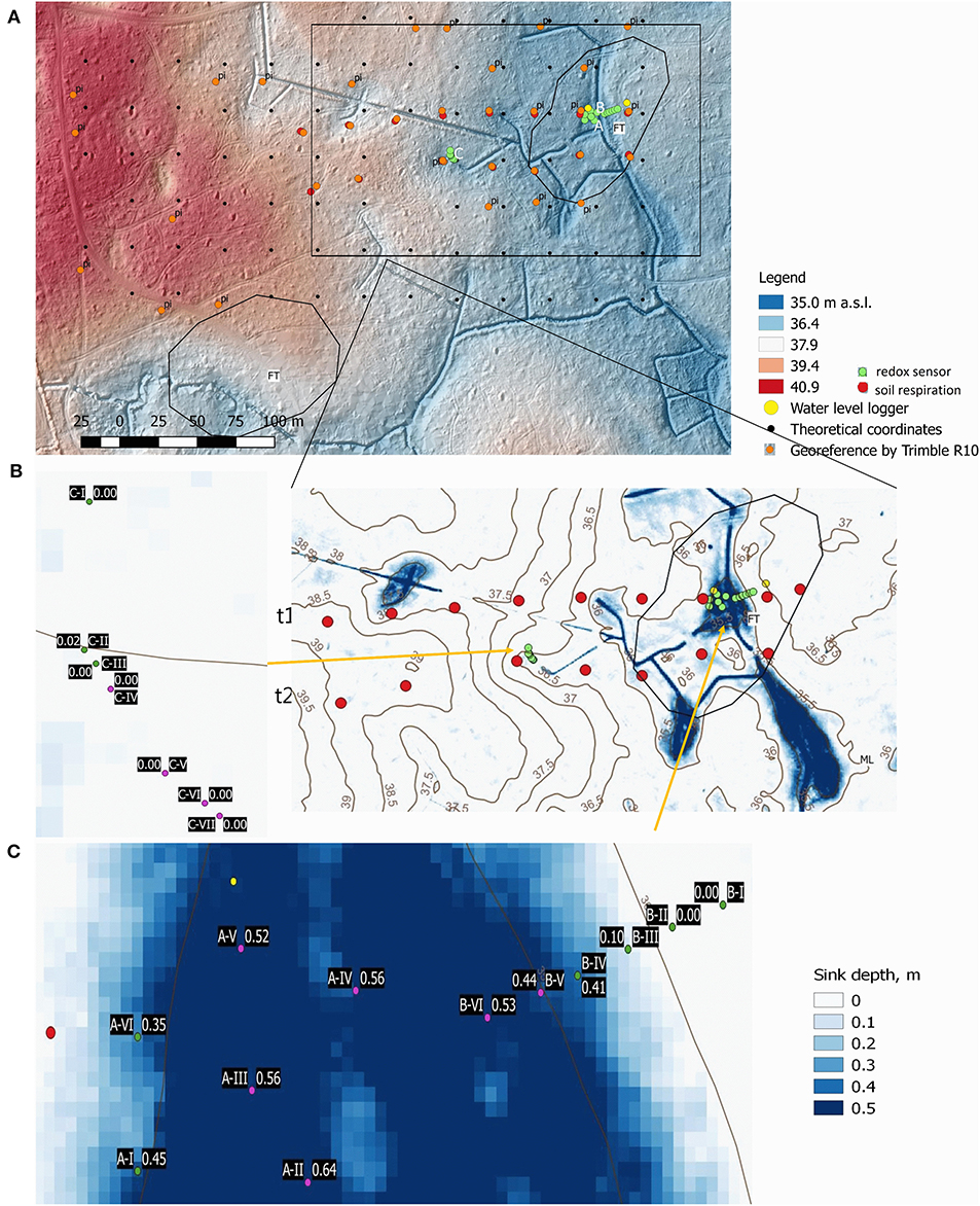
Figure 1. (A–C) (green dots) – redox measurement points. Location of water level loggers: yellow dots. SOC sampling grid (theoretical coordinates): black. Same grid positioned by Trimble R10 (poles identified are labeled with “pi” label): orange dots. Soil respiration points: red dots. (A,B) Redox measurement points: green dots. The background is the DEM 0.4 m. Black line polygons – FT – peat signature from legacy map. Lower maps: Measurement of redox potential (Eh) in groups of three Pt sensors (dots with labels: group ID and depth of TD, cm. Cyan color: anaerobic sequences observed during growing season). Soil respiration and litterfall measured at red points in east-west lines marked t1 and t2. Background – Bluespot map with elevation contour lines (brown, m.a.s.l.).

Two east-west transects (red dots, Figure 1) with a total of 15 points in the 30 m grid were selected for soil respiration measurements every 2–3 weeks during the years 2014–2017. Data from 2016 and 2017 were used for the present study. These points were located within SW coordinate 55.485° N 11.641° E, and the NE coordinate was 55.486° N 11.644° E extending about 50–250 meters in westerly direction away from the EC tower, and an elevation range of 35.93–38.75 m a.s.l. The horizontal distance to nearest ditch was on average 13.8 m (range 4.1–35.8 m) and the vertical distance to nearest ditch was on average 0.85 m (range 0.56–1.51 m), Figure 1. The two transects were georeferenced using a Trimble Pathfinder XT (limited set of ground correction signals) and a new Trimble R10 (Trimble, Sunnyvale, CA, USA) with integrated Global Navigation Satellite System (GNSS). In December 2018 only 19 of the marker poles could be located, and many were in a rather decomposed state. Others possibly had been buried under litter or were hidden under slash from harvested trees.

To estimate the variability of aboveground carbon inputs, litterfall was collected monthly in litterfall collectors (ø 0.5 m, height 1.5 m above ground, n = 2 per plot), dried at 55°C to constant weight, sorted to leaf and non-leaf fractions, and weighed to estimate total annual litterfall, L_abg, in kg C m⁻² representing the aboveground carbon input to the soil in the two soil respiration transects (red dots, Figure 1).

The sampling locations of the SOC grid, soil respiration transects, Eh and water table loggers are shown in Figure 1 and in higher resolution in the lower maps of Figure 1. The positioning of the platinum (Pt) sensors and water level loggers was targeted at representing transitions from aerated mineral soil over wet mineral soil to organic soil near ditches at three locations, A, B, and C (Figure 1). Positioning done by compass, measuring tape and trigonometry from a known ground position and verified by GPS/GNSS (Trimble R10). Next to the Pt sensor groups, freshly sanded iron rods were placed to allow for reaction of the iron rod with the soil environment to show zones of low Eh (R), and shifting Eh (O/R) (Supplementary Figures 1.1, 1.2).

At a high and low elevation point crossing the border of a TD in the easterly end of the Northern transect (t1) the water tables were logged at a bi-hourly interval with U20 loggers (Onset computers, Bourne, MA, USA) with a reference subjected to atmospheric pressure. Manual gauging of the water table with a measuring tape was done every 2nd month and these data were used for calibration of the logged water table data.

Maps and Remote Sensing Data Characterizing the Study Area

The DEM was generated from LiDAR classified ground point data with a resolution of 0.4 m × 0.4 m and supplied as open data by the Danish ministry of Energy, Utilities and Climate and based on a national scanning campaign (sdfe.dk; Kortforsyningen.dk, 2015). The elevation (z-coordinate) from the elevation raster dataset was sampled for the points in Figure 1 (Qgis 2.18 point sampling tool plugin). Further, it was used to derive slope (Qgis 2.18) and the depth of topographical depressions using the algorithm “Filled sink” (Saga GIS 2.3.2; Planchon and Darboux, 2001). The Filled sink algorithm finds topographic depressions by first filling infinite amounts of water to the DEM and then removing it using the restriction that TDs extend to where a continuous path from a lower point in 8 surrounding cells can be defined (Planchon and Darboux, 2001). With a spatial resolution of 0.4 m, it means that they can be as small as one cell allowing for studying microrelief.

The soil parent material was glacial till with some peat-filled topographic depressions as indicated by a map designating parent material polygons at a depth of about 80–100 cm in 1:25.000 (GEUS, 2015). The map is based on the inspection of augered samples with respect to sediment type and interpretation of deposit type. Polygons of different parent materials were delineated during the 19th and 20th centuries by using topographic maps and aerial photo interpretation. The maps were digitized in the 1990'ies, and transformations have caused ~5–10 meters of spatial bias. The uncertainty of polygon boundaries can be several meters (50–100 m), depending on the type of parent material and the landscape (GEUS, 2015).

To aid the interpretation of water table and Eh data, precipitation data for 2016 and 2017 for the 10 × 10 km grid cell “10,449” and “20,146” were obtained from the Danish Meteorological Institute (novana.dmi.dk).

The spatial extent of the crown cover of beech stand is essential for assessing the amount of incoming solar radiation to the forest floor, since the leaf mosaic of beech almost prevents the penetration of light. It was quantified (percent of area in 25 × 25 m pixels) by using the Danish Biomass map (Nord-Larsen et al., 2017) which is based on the same LiDAR point cloud data that was used for the DEM (SDFE, kortforsyningen.dk) in the analysis of SOC stocks in the grid.

Measurement of SOC Stocks, and Soil Respiration and Eh

SOC stocks at a depth of 0–40 cm were calculated according to equation (I) from one soil core per grid point taken with a soil corer (type Eijkelkamp ø 8.3 and 8.7 cm. Agrisearch Equipment BV, Giesbeek, The Netherlands) in the 30 × 30 m grid in depth segments, i = 0–5, 5–10, 10–20, 20–30, and 30–40 cm. The forest floor was sampled quantitatively by collecting all O-material within a 25 × 25 cm frame. The soil core was photographed in order to document and describe indicators of drainage and these were visually interpreted, Supplementary Figure 1.3. Mottling of high value/chroma Munsell colors and Manganese concretions (MnO₂) indicated pseudogley due to stagnic soil water. Gley colors (grayish or whitish hue) indicated gley from a water table, and/or the color of the unweathered parent material, calcareous till (CaCO₃).

$\begin{array}{l}(\text{I})\text{ SOC }(\text{kg C}{m}^2)={\displaystyle \sum _{{layer}_i}}\left[\text{C},{mgg}^{-1}\right]\times \left[\text{BD},\text{ t }{m}^{-3}\right]\\ \times \text{V }{m}^3{m}^{-2}\end{array}$

The organic carbon (OC) concentration was calculated as total carbon (TC) measured by dry combustion by deducting carbonate-C. The carbonate-C content was analyzed by determining the evolution of CO₂ upon treatment with phosphoric acid (C-MAT 550, Strohlein GmbH, Viersen, Germany; cf. Schrumpf et al., 2011).

Soil respiration (R_soil) consists of autotrophic respiration by plant roots, R_a, and heterotrophic respiration by soil living organisms, R_het; we used it as an indicator of the magnitude of soil processes and environmental controls on it, i.e., soil water content and soil temperature. Further, we make a crude assessments of R_het by assuming annual R_a to be 50% of the average annual R_soil (Brændholt et al., 2018) for the 6.6 ha area in order to assess dC_soil.

Soil respiration was measured manually as soil CO₂ efflux along the two transects (red dots, Figure 1) using a portable 8100–102 10 cm survey chamber connected to a LI-8100A Automated Soil CO₂ Flux System (LI-COR Environmental, Lincoln, Nebraska, USA). Measurement spots were permanently installed soil collars, inserted 4 cm into the soil. Each of the 15 locations along the transect contained 3 soil collars giving a total of 45 plots. The R_soil plots contained litter but no aboveground plant component. The measurements were performed at an interval of 2–3 weeks, where R_soil was measured once per plot with a chamber closure time of 150 s. R_soil measurements typically were carried out on 1 day between 09:00 and 16:00 CET. Fluxes were calculated on a time and area basis using the LI-COR software (LI-COR Environmental, Lincoln, Nebraska, USA). Alongside R_soil, soil temperature and soil moisture content were measured at a depth of 5 cm. Soil temperature was measured at one point 1 cm from the soil collar. Soil moisture was measured by a soil moisture probe (TDR, ThetaProbe ML2x, Delta-T Devices Ltd, Cambridge, U.K.) at four points evenly spread around the soil collar at a distance of 10 cm. The average soil moisture content of those four measurements was taken as the soil moisture content of the plot. Annual average R_soil in kg C m⁻² yr⁻¹ was calculated (equation II) as the average of the measurement days during 2016 and 2017 in μmol CO₂ m⁻² s⁻¹ with unit conversion:

$\begin{array}{l}(II)R_{soil}\left(kgC{m}^{-2}\right)=R_{soil}\left(\mu molC{O}_2{m}^{-2}{s}^{-1}\right)\\ \times 12gC{mol}^{-1}\times {10}^{-9}kg{\mu g}^{-1}\times 31.536\\ \times {10}^{6}s{yr}^{-1}\end{array}$

The soil Eh (Fiedler et al., 2007) in the upper root zone were studied in three different elevation gradients representing wet to dry soil with surface elevation range 35.31–35.45 m a.s.l. (location A), 35.41–36.36 m a.s.l. (location B), and 36.39–36.65 m a.s.l. (location C), Figure 1. Location A was mostly peat (organic soil) about 40 cm deep with no tree vegetation, but also wet mineral soil (groups I and VI), whereas lower parts of B and C were SOC rich wet mineral soil. The distance between measurement points was 2–3 meters. At A, B, and C, 18 Pt sensors in groups of two to three were placed 20–25 cm from the soil surface into the ground and connected to data loggers. Location A had a radius of maximum 5 meters defined by the length of the cables, whereas B and C had a length of 10 meters also limited by cable length, where, in terms of measurement quality, “shorter is better”. Location A was a fen in the lowest part of the study area. The end-to-end slope of location A was 3.5°, and the slope of location B was 5.4°. Location C was a line transect intersecting a micro catchment upslope of a ditch with a slope of 1.4°, Figure 1.

The Pt sensors were connected to a Hypnos IV (MVH Consult, Leiden, Netherlands; Vorenhout et al., 2011) along with a Ag⁰/AgCl reference electrode (equilibrium E_ref 222 mV in 4 M KCl, q-i-s.net, Netherlands; Vorenhout et al., 2011). The third logger was based on a digital voltmeter and digital relays that connected the sensor and the reference electrode with the voltmeter for 500 milliseconds of measurement once per hour. This logger was controlled by a Python 3 protocol on a Raspberry Pi with 12V power supply (Cperf Aps, Holte, Denmark). The Eh of the soil matrix measurements (E_meas) was defined relative to the standard hydrogen electrode by adding the equilibrium potential (E_ref) of the reference electrode process (equation III).

$\begin{array}{l}{(III)E}_h=E_{meas}+E_{ref}\end{array}$

Analysis of variance of SOC stocks and annual average soil respiration with terrain variables and other regression analyses were carried out in proc GLM, TTEST and CORR, SAS 9.4, SAS Institute. GIS analyses were carried out in QGIS 2.18 (tools: point data extraction, slope, raster calculator) and SAGA Gis 2.3 (Filled sink). Eh data were used along with water table measurements for visual interpretation of the temporal and spatial boundaries between aerobic and anaerobic soil environment (Figure 1) with potential impact on SOC stocks and soil respiration.

Results

Soil Development and SOC Stocks

The map of predicted SOC stocks is shown in Figure 2. The mapped SOC stocks reflect the topographical depressions of varying size. Within the 6.6 × 10⁴ m² study area, 12 of the 73 sampling points were located within topographic depressions defined as the difference of the estimated sink surface (when filled) and the elevation of the sink point when not filled. “Filled sinks” covered an area of 18.9% ranging from a few centimeters of sink depth to 0.78 m near a ditch. The map of parent material (GEUS, 2015) indicated 8.2% peat cover in the study area (two black circles, FT signature in Figure 2). The delineation of the peat polygones only partly matched the carbon rich point observations in the 30 m grid. Artifacts such as ditches, roads and stumps that were not sampled have biased SOC estimates.

FIGURE 2

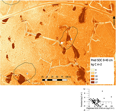
Figure 2. SOC stock estimates (0–40 cm) and residual plot (insert) from GLM upscaled with DEM 0.40 cm and previously mapped peat area, (black line polygons: FT–signature for peat, ML–loamy till, GEUS 1:25.000). Equation: SOC, kg C m⁻² = 45.95 – 0.368*slope(degrees) – 0.951* elevation (m a.s.l.) – 503.2*sink depth (m) + 14.6* elevation*sink depth. Mean standard error of individual prediction (94 grid points) was 2.45 kg C m⁻² (std 0.13, range 2.4–3.2 kg C m⁻²). Ditches, tree stumps and roads are artifacts, not represented by sampling and thus biased.

SOC Stocks 0–40 cm

The A horizon in the soil cores of the SOC grid was a dark brown or black mull, 10–40 cm deep (see example photos in Supplementary Figure 1.3). Signs of pseudogley processes were seen 25–50 cm below the surface of the mineral soil. Gley was observed near ditches in depths ranging from 15 to 40 cm under a deep A horizon. The calcareous parent material of the C horizon was in most points seen within the depth of 50–60 cm across the study area.

The elevation of the grid points (m a.s.l.), the slope (degrees), the depth of TDs (Sink depth, cm), and the interaction term between elevation and sink depth explained SOC stocks by fairly equal values of sums of squares (type III) in analysis of variance (R² 0.55, mean = 8.9 kg C m⁻², RMSE = 2.4 kg C m⁻²). SOC stocks outside topographic depressions (8.4 ± sem 0.3 kg C m⁻²) were significantly smaller (P < 0.01) than within TD areas (11.9 ± sem 0.5 kg C m⁻²).

Two of the explanatory variables, elevation and depth of TD were negatively correlated (r= −0.30). The explanatory variable slope at the SOC sampling points was correlated with elevation (r = −0.16) and depth of TD (r = 0.57). These predictors were deemed necessary in the linear model and thus included. Residual error (observed – predicted) is visualized in the Figure 2 insert plot. The statistical model seemed to overestimate low SOC values and underestimated medium to high values except from the highest observations that are carbon rich points in or near TDs. The topographical depressions and ditches were clearly visible on the hill-shaded elevation model. The ditches, roads and stumps caused some artifacts in the SOC estimates, when interpolation used the 0.4 × 0.4 m DEM raster, but they are clearly visible. Also, a few extreme values from −8.7 kg C m⁻² to 74 kg C m⁻² in the upscaled raster suggested that a cutoff at meaningful boundaries for SOC stocks (Figure 2) would be needed.

SOC Stocks in Forest Floor and Litterfall

Looking at the forest floor C stock only (data not shown), the mass of organic carbon in the SOC grid above 39 m a.s.l. was 0.22 ± 0.1 kg C m⁻², on average 35% lower than the eastward end of the transects holding 0.34 ± 0.4 kg C m⁻² (heteroscedastic t-test, P = 0.03). The crown cover in the forest stand during the summer of 2015 varied from 63 to 92% of the surface area among the transect points. Within the observed crown cover range a 25% decline in crown cover corresponded with a 25% decline in litterfall C in a linear regression (R² 0.33). Higher crown cover also coincided with higher forest floor SOC, but for lower crown cover there were both high and low forest floor SOC values (data not shown). Leaf litter inputs to t1 and t2 transect points on average amounted to 0.18 kg C m⁻² (SD 0.03) in 2014–15 and 2015–16 (June through May) almost equaling the forest floor SOC stock, and indicating a fast turnover of the litter in the forest floor. The measured litter fall was not related to soil respiration nor did it show a trend along the two transects.

Accuracy of SOC Sampling Point Location

The theoretical coordinates were used for the point sampling of elevation, slope and depth of TDs from the DEM as the drift of the sampling point coordinates and identification of pole markers in the grid could not be fully elucidated. The bias introduced by this was assessed: The elevation bias of the 19 sampling points with identification of the pole was unbiased (on average 0.05 m) with minimum – 0.46 m and maximum 0.50 m elevation difference on the DEM for the x, y offset between the theoretical coordinate and the measured coordinate. However, this was important for the SOC stock estimation in the grid (Figure 2 insert). The highest residual in the SOC estimates all were points near TDs. The average Trimble measurement error on the horizontal coordinate (x, y) was 0.46 m (range 0.01–1.5 m) and the vertical (z) coordinate error was 0.67 m (range 0.01–2.26 m) according to the instrument. However, the difference between the DEM and the GNSS elevation (z coordinate) was in some cases 4–7 meters. The use of a DEM for z-coordinate estimation of measurement points in forest is thus the more robust method for elevation determination in this comparison.

Soil Respiration

The mean rate of R_soil ranged from 0 to 5 μmol CO₂ m⁻² s⁻¹ corresponding to 0–5.2 g C m⁻² d⁻¹ with a wider range of extremes during the growing season. The annual average soil respiration was 1.0 kg C m⁻² yr⁻¹ with a range of 0.7–1.3 kg C m⁻² yr⁻¹.

Temperatures as well as R_soil were higher in the 2016 growing season than in 2017, Figure 3A corresponding with a precipitation deficit of −215 mm in 2016 and −71 mm in 2017. Soil water content was on average in the range 25–45% except in June 2016 when it was ~15% across 15 measurement locations in the two transects, Figure 3B. The within-day variation in soil water content did not seem to have a strong effect on the soil respiration, judged by the width of variation in the soil respiration.

FIGURE 3

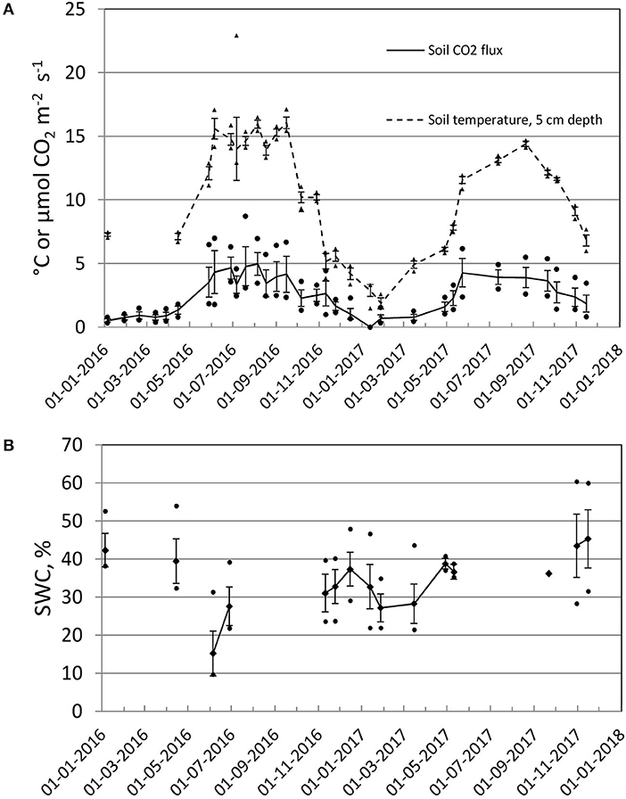
Figure 3. (A) Soil temperature (triangle) and soil respiration (dot) measured at 2–4 week intervals during 2016 and 2017, (B) Volumetric (%) soil water content (SWC) in topsoil (0–5 cm) during 2016 and 2017. The overall mean was 34.3% with a range of 9.7–60.4%.

The sampling collars were mostly under a tree crown, but depending on the solar trajectory during the day, there could be periods of full sun or full shade. The within-day variation in soil temperature was highest in summer, fall, and early winter 2016, Figure 3A, which gave a positive correlation between R_soil and soil temperature between plots after this relatively dry summer (numerical value of Pearson correlation, r > 0.5 in 3 out of 12 days; range 0.5–1.8°C, Supplementary Figure 1.4). This was not the case during the winter 2017 where the range in temperature was smaller. R_soil was higher at lower elevation within the same day in spring, summer and fall (r < −0.5 in 11 out of 31 measurement days; range 35.7–38.7 m a.s.l.).

The depth of topographical depressions relative to the theoretical surface of a pond in the DEM model were different from zero in 6 out of 15 points and varied from 0 to 0.22 m in depth. The transect points (red points in Figure 1) thus avoided the deepest parts of the study area. The correlation between soil respiration and depth of the TD was positive, and higher than 0.5 at 3 measurement days in spring and early summer (Supplementary Figure 1.4).

Soil respiration at the 0.4 × 0.4 m resolution (Figure 8) was estimated by using the predicted SOC 0–40 in Figure 2 with the regression parameters from the relation between soil respiration and predicted SOC 0–40 cm relation based on the 15 points in the two transects (see parameters in the caption for Figure 7D).

Soil Eh at 20 cm Depth Below the Surface

Soil Eh showed annual variations that were related to the depth of the soil water table (aerobic; around 800 mV when the water table was deep) and precipitation (rapid drops in Eh to around 0 mV after rain during summer). This is illustrated by Figures 4–6. The redox measurements inside topographic depressions (all of location A, lower three points in location B, no points in location C) showed a mostly anaerobic soil environment at 20 cm depth, unless on a slope, and the low Eh was closely linked with high water table. Location C was not within a TD but still had low Eh during spring. Nearly flat terrain near a ditch is therefore an important additional indicator for water saturation and low Eh.

FIGURE 4

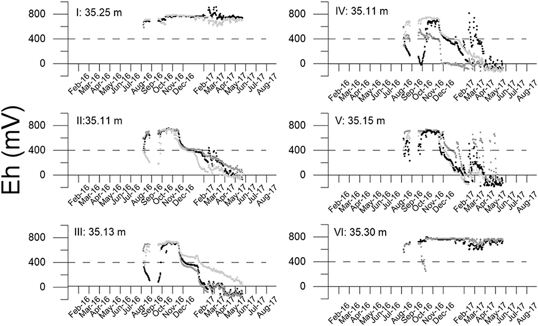
Figure 4. Redox measurements in location A, the fen. Individual sensor location marked, m a.s.l. and in Figure 1. Dotted line – 400 mV reference for aerobic/anaerobic soil environment.

In the fen (location A, 35.4 m a.s.l), a real water table was always present, on average 35 cm below the surface (range 0–70 cm below surface). The water table was fed by the ditch system and could fill up quickly after a rain event, (see water table in Figure 5B-VI). At this location, the organic soil did not support the growth of beech trees; instead nettles (Urtica dioica L.) prevailed signaling abundant nitrate. The rapid drops in Eh occurred during spring, after which stable, strongly reducing conditions in the peat (Eh around 0–200 mV) prevailed during 2017, whereas the two groups (I and VI) sitting 20 cm higher in mineral soil on a slope were mostly in the aerobic range higher than 400 mV.

FIGURE 5

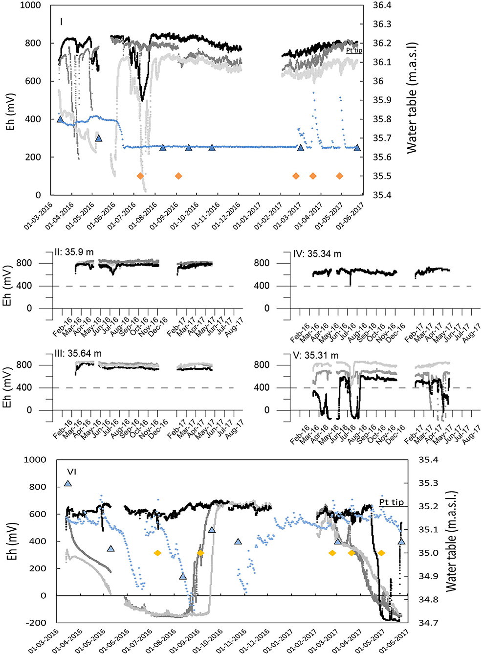
Figure 5. Eh and water table fluctuations during March 2016 to June 2017 at the Eh measurement points in location B adjacent to the water loggers. I: Upslope position 36.4 m a.s.l.; II–V. Pt group positions on the slope; VI low area near ditch 35.4 m a.s.l. The top end of axis2 (water table) indicate the soil surface. Pt tip marked on axis2 shows the platinum sensor position, m a.s.l. The black and the two gray lines indicate the triplicate Eh measurements, mV, vs. date (axis 1). Yellow diamonds: 20+ mm rain events (marks the date on x-axis). Blue dots (axis 2): Water table by Hobo U20 logger and manual water level measurement (blue triangles – dry from July 16 to March 17) and short periods thereafter.

The upslope nearly flat position in Figure 5B-I had a seasonal water table in spring that fluctuated between 50 and 70 cm below terrain (36.6 m a.s.l.) and was otherwise deeper than 75 cm below surface during summer. Rain events with 20+ mm rain on July 10th, and September 4th increased the Eh at one sensor; the other two measured a decreasing Eh, illustrating the microscale variability of Eh, possibly due to variable water filling of soil pores. The most constant aerobic environment was on an 8° slope (795 ± 39 mV) where anoxic water was probably never in contact with the Pt sensors, Figure 5B-II–IV. The soil water was most likely never stagnant due to the possibility of a rapid lateral subsurface movement on the slope forced by gravitation, Figures 1, 5.

The iron rods in the downslope groups of the B location (B-V and B-VI in Figures 1, 5) had a thick, strong red iron oxide coating, indicating the transition zone between the oxic and anoxic environment. Fe in the interflow water had precipitated under aerobic conditions in the oxic zone, (Supplementary Figure 1.1). In area C there were no signs of significant amounts of interflow water in the zone of shifting redox environment, i.e., no indication of iron oxides precipitating from laterally transported Fe (Supplementary Figure 1.2).

Eh drops from around 600 mV (aerobic) down to 0 mV (anaerobic) occurred during winter and spring in the nearly flat area (Figure 6C-II–VI, slope 1°) in line transect C with an increasing duration of low Eh closer to the ditch, C-VII.

FIGURE 6

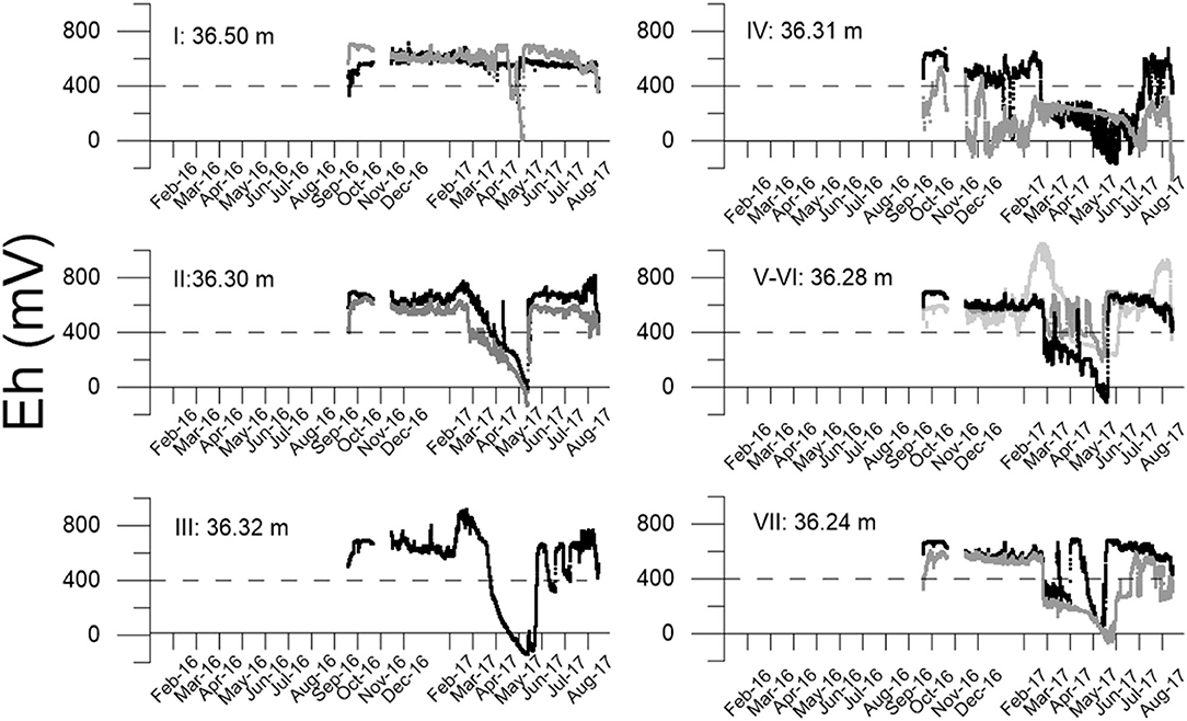
Figure 6. Redox measurements in location C. Individual sensor location marked, m a.s.l. Dotted line – 400 mV reference for aerobic/anaerobic soil environment.

Note that the Hobo water table sensors drifted in comparison with manual measurements of the water table, Figure 5B-I–VI, causing uncertainty in the actual level of the water table. However, peaks in the water table immediately after rain events were observed as peaks in the continuous logging of the water table, e.g., during spring 2017, Figure 5 (blue dots, axis 2). The Pt sensors indicated on axis2 (I–VI, Figure 5B) were submerged under the water table due to inflowing water from the catchment for most of the time, especially during spring and early summer in both years. This caused the Eh to drop to strongly reducing conditions in the range −200 to 0 mV for long periods.

Synthesis of SOC, Respiration, Soil Eh, and Water Table Measurements

SOC stock measurements and respiration measurements were co-located (with some positioning uncertainty) in transects t1 and t2. Unfortunately, there were no soil respiration measurements directly paired with Eh measurements in the study, nor were respiration measurements at the lowest and highest position of the elevation range available.

C-rich points did not have higher than average C respiration per kg SOC. The observed SOC stock range was 6.4–24.4 kg C m⁻², Figure 7A. When using the modeled SOC stock for 0–40 cm soil depth based on DEM covariates sampled by the GNNS positioned respiration points, the SOC stock range was more narrow with a predicted range of 7.4–13.8 kg C m⁻², Figure 7D. This was partly due to the positioning offset (Figure 1) and partly due to regression to the mean caused by noise in the data. Consequently, the rate of soil respiration with SOC seemed to be much steeper: 0.06, (Figure 7C, vs. 0.02 kg C m⁻² yr⁻¹ per kg SOC, Figure 7A). When excluding the 24.4 kg C m⁻² value with uncertain location the regression slope based on observed SOC data was 0.045 kg C m⁻² yr⁻¹ per kg SOC. The forest floor plus the 0–20 cm SOC pool (approximate depth of Eh measurements) gave the best fit with a rate of 0.06 kg C per kg SOC in the range 4–11 kg C m⁻² (R² 0.65, Figure 7C. The equation for Figure 7D based on estimated SOC (Figure 2) was used for interpolation of C respiration illustratied in Figure 8, and yielding 96% of the C respiration predictions within 0.6–1.4 kg C m⁻² yr⁻¹.

FIGURE 7

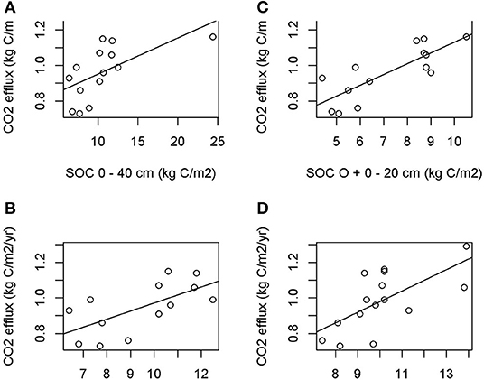
Figure 7. Average soil respiration (2016 and 2017), kg C m⁻² yr⁻¹ vs. (A) measured SOC, kg C m⁻² (theoretical grid) R² = 0.37. α = 0.75 ± 0.01, β = 0.020 ± 0.008; (B) same as a), but without uncertain 24.4 kg C m⁻² observation R² = 0.42. α = 0.52 ± 0.01, β = 0.045 ± 0.016; (C) vs. measured SOC in forest floor + 0–20 cm mineral soil (theoretical grid) R² 0.65, α = 0.53 ± 0.09, β = 0.060 ± 0.013, and (D) predicted SOC 0–40 cm using the GPS/GNSS coordinates at the respiration plots. R² = 0.44 α = 0.38 ± 0.19, β = 0.060 ± 0.020).

FIGURE 8

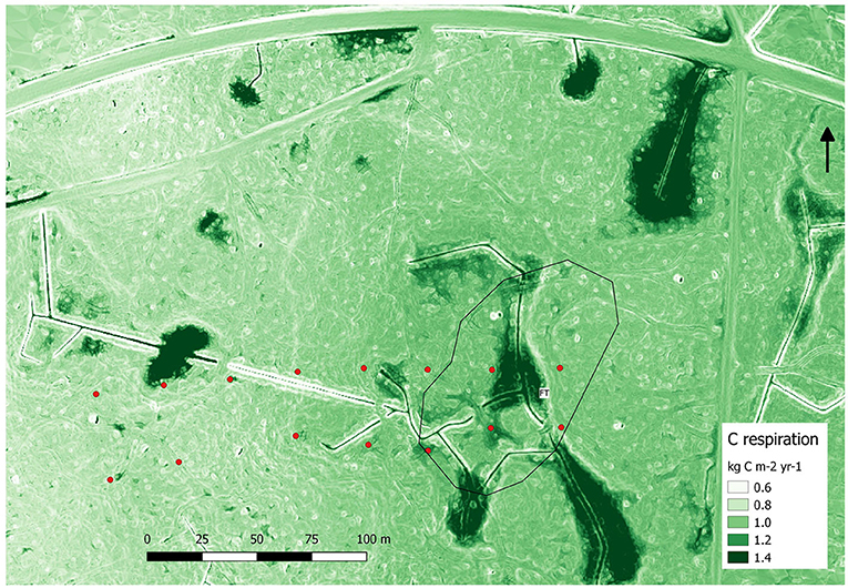
Figure 8. Predicted soil C respiration, kg C m⁻² yr⁻¹ from equation in Figure 7D. Red dots: respiration measurement points.

Discussion

The Use of Detailed DEMs for a More Accurate Activity Data Mapping of SOC, Respiration and SOC Stock Change Over Time as Related With Soil Type

The SOC accumulation at this site clearly reflected the microrelief (based on 73 grid points), with significantly higher SOC stocks to depth 40 cm inside the TDs. The same trend was seen for the subset of 15 points with respiration measurements (not tested due to limited number of data points). Generally, Hapludalfs in Danish forests on well-drained sites hold 3–6 kg C m⁻² to 20 cm depth (Vejre et al., 2003) in on average 20 cm deep A-horizons, but at this site the corresponding average SOC stock was 7 kg C m⁻². The study area also had presence of soils of the Aquic subgroups of the Argiudolls (Østergård, 2000) where hydromorphism causing SOC accumulation due to slow decomposition is important for the soil formation.

The high-resolution DEM was used for extraction of elevation data and the DEM derivatives slope and depth of TD (“Filled sink,” Saga GIS). We here chose to study data collection challenges and new possibilities for more accurate mapping of soil SOC stocks and soil respiration offered by high-resolution DEMs at one of the sites in the ICOS network quantifying terrestrial GHG balances. The terrain covariates were combined with measurements of soil carbon stock, soil respiration, water table, and Eh data evaluated as mostly aerobic or anaerobic in field installations. Such high resolution elevation data have otherwise been unavailable or very hard to get from previous maps and field measurements. The elevation data from GPS and GNSS were very uncertain showing an error of up to 4 meters in the z direction. Sampling from the LiDAR based DEM was a more accurate option, since it can estimate elevation (z) with 0.01 m resolution and 0.05 m uncertainty (GST, 2015), whereas the horizontal error is only 0.15 m. The DEM is based on 4–5 scatter points per square. However, noise caused by lying forest floor objects such as stumps and fallen decaying stems cannot be ruled out. Accurate x, y coordinates are a prerequisite for accurate sampling of the z-coordinate from the LiDAR based DEM. This was demonstrated by the actual offsets from the theoretical grid points (Figure 1). Horizontal positioning should be done using GPS or GNSS, or by terrestrial LiDAR or drone LiDAR with a base station.

After 14 years it was difficult to find the marker poles of the SOC monitoring grid. This compromises the use of legacy SOC data, and new sampling of soil in SOC surveys is therefore still needed. Only when accurate and precise field identification (georeferenced) data are available, an accurate resampling of point based SOC stocks can be performed. The SOC estimates in Figure 2 indicate how variable SOC stocks can be at short distance, and the map correctly shows the sharp borders between the mostly aerated upland areas and TDs with higher associated SOC stocks in hydromorphic soils that were are often anaerobic in 20 cm depth. The slope of ditches are outside the range of the sample points and cause artifact values for SOC and C respiration predictions near ditches. Also tree stumps, ditch levees and wheel tracks could be seen on high-resolution elevation models and these were reflected as biased values in estimates of SOC and soil respiration (see Figures 2, 8). Such artifacts could potentially be quantified by designed studies of SOC, soil respiration and Eh measurements and included in the models behind the SOC and respiration estimates.

The model parameters for SOC is thus not robust to extrapolation and are unique for the area. The mechanisms for SOC accumulation i.e., anaerobiosis caused by relief were reflected in the explanatory variables derived from the DEM, and they are generic in soil formation (Jenny, 1941).

Positioning of measurement locations is a limitation for utilizing the high resolution of DEMs for covariate point sampling. Precision georeferencing (±0.5 m for finding physical markers) and perhaps more persistent marking poles need to be developed and become widely used.

The ditch-network could be easily visualized by hill-shading (Figure 1) and the depth quantified by the “Filled sink” routine (Figure 1). The vertical and horizontal distances to the ditch were calculated for t1 and t2, but in this study they were incorporated in the elevation effect on SOC stocks and C respiration.

The use of a high-resolution DEM makes mapping of soil carbon stocks and soil respiration potentially much more accurate irrespective of using the traditional “expert” mapping methods used e.g., in the digitized map of parent materials (which also depend strongly on relief interpretation) or algorithm and covariate-based methods. The use of DEMs and derivatives as a covariate would be directly applicable in the analysis and interpretation of monitoring data used in national forest inventory and greenhouse gas reporting to the UNFCCC. The design of such surveys should focus on covering the extremes of water saturation throughout the year. Here, measurement of redox potential in our study proved to be a robust method for documenting aerobic or anaerobic soil environment at 20 cm depth.

The stated accuracy and precision of the digitized legacy geological map includes a 5–10 m transformation bias (GEUS, 2015) that seemed evidently larger in Figure 2 showing two black circles of the legacy map indicating peat soil clearly offset by 20–25 m from the topographical depressions. The legacy map can be corrected by the Filled sink routine, i.e., blue spot maps, which are available in high resolution with nationwide coverage.

We found that the “Filled sink” (Saga GIS) routine used as a covariate along with the elevation (DEM z value) could separate SOC stocks in upland mineral soils from wet mineral and organic soils. This was indicated by higher SOC stocks, higher water tables and an Eh in the anaerobic domain in the latter. The SOC stocks increased with the depth of the TD. The average SOC estimate for the same site by Schrumpf et al. (2011) with a standard deviation of 2.64 kg C m⁻² (0–30 cm C stock), was here reduced by stratification to a CV (using the model sem) of 4.0% (inside TD) and 3.6% (outside TD) for the 0–40 cm SOC stock. The soils reflecting the area of TDs vs. the legacy map peat area (FT) are not directly comparable, since not all of the TDs were organic soils or even wet soils, but the likeliness of belonging to this group is higher the larger and the deeper and larger the TD is, and with closeness to ditch in a flat position.

Effect of Ditching on Soil Aeration and Loss of Legacy SOC

Ditches are currently quantified by the Tier 1 default value of 2.5% of the area (IPCC, 2014) in the Danish NIR (Nielsen et al., 2020). The area of ditches may now be quantified by analyzing a high-resolution DEM. Further work is needed to assess which of these TDs are actually water-filled and for how long (Hasselquist et al., 2018). Here, direct measurements of ground water tables and Eh in high and low positions were in use for the interpretation of SOC stocks, and the annual soil C respiration. We showed that the lower part of the ditch system was always (during 2016 and 2017) water saturated at an elevation of 35.4 m a.s.l., which would protect peat stored below this depth against aerobic decomposition. The best fit of soil respiration with SOC was therefore Figure 7C with a slope of 0.06 kg C per kg C for the Olfh + 0–20 cm soil pool. C respiration rate data from inside the deeper peat-filled TDs concurrently with Eh and water table measurements would be needed, however to verify respiration rates there. In concordance with this, there was no indication in the data that respiration in the more SOC-rich soils increased per kg SOC, on the contrary the respiration per kg SOC seemed to level off at increasing SOC stocks, Figure 7A. Furthermore, points at lower elevation had higher C stocks in O-horizons, also possibly indicating less earthworm activity due to more frequent water saturation and more litter input via lateral transport (see section Elevation gradient and leaf litter input in relation to SOC). The identification of legacy SOC lost due to drainage cannot be made with the soil C respiration data, but we can show whether the soil was aerobic or not at the depth of 20 cm using the continuous redox data. We examined the relief transition from dry to wet soil across TD borders (location A and B), or near ditches (location C). We could see that anaerobic soil occurred also outside TDs on mineral soil, and that the current water table rarely and only briefly reached the border of the TD in location A at 35.8 m a.s.l (compare with water table curve in Figure 5B-I). When the soil was anaerobic and C-rich, fast C mineralisation due to aerobic respiration did not take place below 20 cm depth, but could happen in the top 20 cm when not flooded. Jauhiainen et al. (2019) reviewed the complexity of describing C balances of forest on organic soils, and stressed the importance of water table measurements to correctly asses the soil aeration status.

In this study the range in measured annual soil C respiration was 0.7–1.3 kg C m⁻² yr⁻¹, Figure 7. The default IPCC emission factor of 0.26 kg C m⁻² yr⁻¹ for drained organic soil would represent 20–33% of the measured annual soil C–respiration, but only 1–2% of the SOC stocks. It also would be smaller than the sum of the annual aboveground inputs (0.18 kg C m⁻² yr⁻¹) plus belowground inputs (not measured in this study). Using soil respiration (autotrophic plus heterotrophic) as an indicator for loss of legacy SOC would therefore require markedly increased soil respiration fluxes as compared to adjacent upland soils to present a clear signal of legacy SOC loss. Both photosynthate inputs and autotrophic respiration could be naturally high in nutrient and SOC rich wet soils that have aerobic top soil in some periods during summer (Figures 1, 4–6) and a net loss would be difficult to measure. Wu et al. (2013) established the GHG balance during 2006–2010 for this site based on eddyflux data, flux chambers and biometric measurements and showed that inputs to the soil could be smaller than the heterotrophic soil respiration. The SOC change in that study was estimated at a small and uncertain net loss of 0.033 ± 0.085 kg C m⁻² yr⁻¹ for the larger eddy flux footprint area of the tower.

Our study shows that this loss could be owing to losses from SOC rich soils in the ditched topographical depressions. A simple stratified soil C balance assuming 50% R_a:R_soil of the mean annual R_soil i.e., R_a 0.5 kg C m⁻² yr⁻¹ would leave R_het a range of 0.2–0.8 kg C m⁻² yr⁻¹ to balance the measured R_soil range (Figure 7). Above and belowground litter input of 0.18 ± 0.03 kg C m⁻² yr⁻¹ (measured) + 0.18 ± 0.05 kg C m⁻² yr⁻¹ (guesstimate) would yield an input of 0.36 ± 0.06 kg C m⁻² yr⁻¹. Area weighing by the estimated average SOC and area of TDs (18.9%) and calculating the dC_soil inside and outside TDs using Figure 7D parametres yielded dC_soil of −0.020 ± se 0.10 kg C m⁻² yr⁻¹ outside TDs and −0.23 ± se 0.10 kg C m⁻² yr⁻¹ inside TDs, on average −0.064 ± se 0.10 kg C m⁻² yr⁻¹ for the 6.6 ha area. The standard error was propagated using relative standard error estimates from the SOC model (4%), the R_soil model (4–5%), and a guessed R_a se of 5%. The calculated annual average SOC loss was larger than the estimate of Wu et al. (2013) covering a larger footprint area of the eddy flux tower. The estimate for the TD areas was close to the IPCC emission factor of 0.26 kg C m⁻² yr⁻¹ for drained organic soils under temperate forest (IPCC, 2014).

In this study we demonstrated that site-specific continuous water table measurements showed immediate response to rain events (F5 and Supplementary Figure 1.5), and that infiltration and hydraulic conductivity properties of the soil should accompany the use of terrain covariates from a high-resolution DEM for wet mineral soil activity data quantification. In landscapes of Latvia with similar low relief, Ivanovs and Lupikis (2018) tested TD algorithms on a DEM with 2 meter resolution, and found good correspondence between wet soils and the filled sink approach, but also showed effects of infiltration and hydraulic conductivities on TD wetness. These could be defined by the origin of the parent material. At the Soroe site dense B and C horizons made lateral water transport plausible, and also the existence of secondary water tables in flat terrain (Figure 5B-I). Our findings for this site thus indicate that data on surface-near groundwater tables and soil infiltration properties are needed to be able to carry out a nationwide upscaling of soil surface wetness as part of SOC stock mapping and a risk assessment for net mineralisation of legacy SOC. The anaerobic conditions demonstrated in mineral soils uphill show that flat slope even outside TDs (Figure 5B-I) can cause stagnant water and low Eh.

The ditched wet mineral soils in TDs and peat soils in the study area currently have a soil drainage regime that is different from the pre-ditching time when the peat formation took place. The 100-yr old ditching system seem to have caused a more oxygenated soil aeration regime in the ditched TDs causing loss of OM (Jungkunst et al., 2008) and subsidence of the surface elevation of the peat cover, but at the same time also may have increased root litter inputs due to improved root production stimulated by influx of nutrients with interflow water. The presence of nettles known for their nitrate affinity indicated abundant nitrate supply (Ellenberg et al., 1992), and could indicate lateral transport of nitrate as well as in situ net nitrification of organic nitrogen when the soil was aerobic.

Long-lasting anaerobic Eh occurred during the growing season in areas lower than 35.4 m a.s.l. (Figures 1, 4). This elevation was 0.3 m above the ditch bottom in the fen basin, and corresponding with the temporally highest water table measurements in the logger well (Figure 5), and also with the depth of observed black color on iron rods (probably reduced manganese and iron compounds caused by water saturation), Supplementary Figure 1.1. In the lower terrain positions (Figure 5B-V,VI) soil had strongly reducing conditions throughout the year except in late summer where water tables and Eh sank rapidly below the redox sensors and then fluctuated up and down. This difference in reaction time of Eh with a slow decrease during spring and early summer in contrast to fast Eh drop in late summer may be due to a temperature effect on soil Eh, i.e., that microbial activity at higher temperature causes a faster drop in Eh. Similar to our observations, in a study by Vaughan et al. (2009) only 2 days were required to move from oxic to anoxic Eh when soil temperature was higher than 9°C.

The Eh measurements showed seasonality in the way that locations closest to the ditches were anaerobic for most of the spring and early growing season at the depth of 20 cm (e.g., Figures 4A-II–V, 5B-V,VI, 6C-IV–VII). Thus, tree root respiration and aerobic heterotrophic soil respiration would be impaired by the lack of oxygen and by CO₂ accumulation at the depth of 20 cm in soil in most years, similar to a study in a Harvard Forest fen (Davidson et al., 1998). The actual net mineralisation of C may depend on the available nutrients (nitrogen and phosphorus) of the organic matter (Mettrop et al., 2014; Webster et al., 2014) and content of phenolic compounds (Wang et al., 2015). Being a nutrient rich site (Østergård, 2000), the aeration caused soil respiration to exceed the rate per kg C observed in the more upland measurement points in Figure 1.

Elevation Gradient and Leaf Litter Input in Relation to SOC

The pattern of soil C stocks increasing from 7 to 8 kg C m⁻² at high elevation to >11 kg C m⁻² at low elevation (Figure 2) could be related with leaf litter inputs and secondary distribution of the aboveground litter by wind. The spatial pattern in the data was enforced by the regression model (see Figure 2 insert) with positive residuals at low SOC stocks. However, the variation in aboveground litter inputs in t1 and t2 did not seem to be affected by redistribution of aboveground litter fall caused by unidirectional wind transport. Yet, the forest floors had higher SOC stocks at low elevation, but not within TDs. The transects t1 and t2 did not extend into the western part of the stand with significantly lower O-horizon C stocks. Measurements of litter fall there, and of lateral litter transport (Staelens et al., 2011) would strengthen a conclusion in this question.

Differences in O-horizon C stock also may be attributed to differences in bioturbation activity. The population of anecic earthworms, e.g., Lumbricus terrestris L., may be smaller and less active at low elevation closer to the ditches due to water saturation and thus lack of oxygen for their respiration.

We cannot disentangle the possible effect of increased aboveground litter input due to lateral transport of litter, and of soil fauna impediments on forest floor SOC stocks caused by shallow water tables. They would both cause larger and more shallow SOC stocks (due to lack of bioturbation and impeded C mineralisation) in TDs and at low elevation corresponding with the observed pattern of soil profiles (see example in Supplementary Figure 1.3).

Implication of Accuracy and Precision of Coordinates for Legacy Soil C Data

The high-resolution DEM's made from LiDAR data offer great detail and options for calculating terrain indices that can help describing the soil environment. The direct visualization of ditches by the hill-shade photo is an obvious improvement of detail and useful data, since closeness to ditches is associated with higher SOC stocks in NFI data (Callesen et al., 2015). The unknown accuracy and precision in georeferencing of legacy soil data (Vanguelova et al. 2016) is a well-known source of uncertainty when combining legacy soil data with remote sensing data. In our study, the SOC sampling points had been marked by poles, that could be found in only 25% of the cases, and the bias of the theoretical coordinates was quantified by the use of GPS/GNSS technology. However, the GPS/GNSS elevation measurement under forest cover was highly uncertain. Therefore, a permanent marking is preferred for the most optimal x, y, z positioning under forest cover. Correct georeferencing of SOC sampling site and respiration measurement site showed to influence results, Figure 7 (i.e., the 24 kg C m⁻² observation was a potential outlier, compare the effect of omitting the point in Figures 7A,B). Linked to this, the use of a modeled SOC value instead of a measured value doubled the respiration rate per kg C, and modelers should be aware of the more narrow range of predicted values often observed in noisy data. More soil respiration data from peat soils along with water table and redox measurements would strengthen our conclusion that ditching seemed to cause loss of legacy SOC at the time of the study.

Conclusion

Here, we could for the first time explore the suitability of a high-resolution DEM together with continuous measurements of Eh for locating inland wetland mineral soils, their SOC stocks and soil respiration. Soil organic carbon accumulation and soil respiration varied across the forest site due to local and seasonal soil water saturation caused by a combination of topographical depressions and lateral water flow due to low porosity of the underlying Bt horizons and compact calcareous till in the C horizon. At this site the “Filled sink” algorithm, slope and elevation using a DEM with 0.4 meter pixel size was useful for prediction of inland wetland mineral soil with elevated organic carbon stocks, and shifting Eh during the growing season. Annual soil respiration was linked with SOC stocks through the relation to elevation, slope and topographic depressions, and was elevated within TDs causing a net loss of 0.23 ± se 0.10 kg C m⁻² yr⁻¹ here, close to the IPCC emission factor for drained organic soil in temperate forest. A low Eh below 20 cm soil depth indicated that SOC deeper than 20 cm may have contributed to soil respiration in SOC enriched areas at low water tables in summer and fall. DEM data and Eh measurements backed up by iron rods indicating the depth to anaerobic soil offer the option to quantify the spatio-temporal extent of aerobic/anaerobic soil processes in inland wetland mineral soils and thus the soil environment that controls exchange of greenhouse gases between the soil and the atmosphere. Accurate georeferences of the sampling grid for SOC was an issue at the high resolution, and so was artifacts such as ditches, wheel tracks and stumps, that should be studied in future research.

Data Availability Statement

The datasets generated and analyzed for this study can be found in the CURIS repository under the University of Copenhagen. For access, please contact the corresponding author.

Author Contributions

IC, KL, and LV conceived the study. IC collected Eh, iron rod and map data, analyzed all data, and drafted the paper. MV and AM assisted with Eh measurement equipment and guidance. All authors contributed to writing the paper.

A file with maps and photos is provided.

Funding

The project gratefully acknowledges funding from the Danish Council for Independent Research | Natural Sciences (DFF – 1323-00182). [Project 2013-2016: Partitioning forest ecosystem respiration by application of novel isotope laser spectroscopy, PI Kim Pilegaard and Andreas Ibrom, DTU https://www.icos-cp.eu/] and from the Danish Innovation Fund and FACCE ERA-GAS [project INVENT, 2017-2020 I reference 7108-00003b].

Conflict of Interest

The authors declare that the research was conducted in the absence of any commercial or financial relationships that could be construed as a potential conflict of interest.

Acknowledgments

Stiftelsen Sorø Akademi, Denmark is gratefully thanked for giving access to the forest area.

Supplementary Material

The Supplementary Material for this article can be found online at: https://www.frontiersin.org/articles/10.3389/ffgc.2020.563355/full#supplementary-material

References

Brændholt, A., Ibrom, A., Larsen, K. S., and Pilegaard, K. (2018). Partitioning of ecosystem respiration in a beech forest. Agric. For. Meteorol. 252, 88–98. doi: 10.1016/j.agrformet.2018.01.012

CrossRef Full Text | Google Scholar

Breuning-Madsen, H., Nørr, A., and Holst, K. A. (1992). Den danske jordklassificering. Hans Reitzels Forlag: København [In Danish].

Buol, S. W., Hole, F., McCracken, D., and Southard, R. J. (1997). Soil Genesis and Classification. 4th Edn. Ames, IA: Iowa state university press.

Google Scholar

Callesen, I., Stupak, I, Georgiadis, P., Johannsen, V. K., Østergaard, H. S., and Vesterdal, L. (2015). Soil carbon stock change in the forests of Denmark between 1990 and 2008. Geoderma Reg. 5, 169–180. doi: 10.1016/j.geodrs.2015.06.003

CrossRef Full Text | Google Scholar

Christiansen, J. R., Gundersen, P., Frederiksen, P., and Vesterdal, L. (2012). Influence of hydromorphic soil conditions on greenhouse gas emissions and soil carbon stocks in a Danish temperate forest. For. Ecol. Manag. 284, 185–195. doi: 10.1016/j.foreco.2012.07.048

CrossRef Full Text | Google Scholar

Davidson, E. A., Belk, E., and Boone, R. D. (1998). Soil water content and temperature as independent or confounded factors controlling soil respiration in a temperate mixed hardwood forest. Glob. Chang. Biol. 4, 217–227. doi: 10.1046/j.1365-2486.1998.00128.x

CrossRef Full Text | Google Scholar

Ellenberg, H., Weber, H. E., Düll, R., Wirth, V., Werner, W., and Paulißen, D. (1992). Zeigerwerte von Pflanzen in Mitteleuropa. Scripta Geobotanica 18, 1–248.

Google Scholar

Fiedler, S., Vepraskas, M. J., and Richardson, J. L. (2007). Soil redox potential: importance, field measurements, and observations. Adv. Agron. 94, 1–54. doi: 10.1016/S0065-2113(06)94001-2

CrossRef Full Text | Google Scholar

GEUS (2015). Jakobsen, P. R., Hermansen, B. and Tougaard, L. Danmarks digitale jordartskort 1:25000, Version 4.0. Rapport 2015/30. Geological Survey of Denmark and Greenland. Available online at: https://frisbee.geus.dk/geuswebshop/index.xhtml (accessed December 13, 2018) [In Danish].

Greve, M. H., Christensen, O. F, Greve, M. B, and Kheir, R. B. (2014). Change in peat coverage in danish cultivated soils during the past 35 years. Soil Sci. 179, 250–257. doi: 10.1097/SS.0000000000000066

CrossRef Full Text | Google Scholar

GST (2015). Danmarks Højdemodel, DHM/Punktsky. Available online at: https://kortforsyningen.dk/indhold/data (accessed December 28, 2020).

Hall, S. J., and Silver, W. L. (2015). Reducing conditions, reactive metals, and their interactions can explain spatial patterns of surface soil carbon in a humid tropical forest. Biogeochem. 125, 149–165. doi: 10.1007/s10533-015-0120-5

CrossRef Full Text | Google Scholar

Hasselquist, E. M., Lidberg, W., Sponseller, R. A., Agren, A., and Laudon, H. (2018). Identifying and assessing the potential hydrological function of past artificial forest drainage. Ambio 47, 546–556. doi: 10.1007/s13280-017-0984-9

PubMed Abstract | CrossRef Full Text | Google Scholar

Husson, O. (2013). Redox potential (Eh) and pH as drivers of soil/plant/microorganism systems: a transdisciplinary overview pointing to integrative opportunities for agronomy. Plant Soil 362, 389–417. doi: 10.1007/s11104-012-1429-7

CrossRef Full Text | Google Scholar

IPCC (2003). Good Practice Guidance for Land Use, Land-Use Change and Forestry. ISBN4-88788-003-0. Available online at: http://www.ipcc-nggip.iges.or.jp/public/gpglulucf/gpglulucf.html (accessed May 08, 2019).

Google Scholar

IPCC (2006). 2006 IPCC Guidelines for National Greenhouse Gas Inventories. Volume 4: Agriculture, Forestry and Other Land Use. Available online at: http://www.ipcc-nggip.iges.or.jp/public/2006gl/vol4.html Aalde et al. Chapter 2: Generic Methodologies Applicable to Multiple Land-Use Categories and Aalde et al. Chapter 4: Forest land (accessed May 08, 2019).

IPCC (2014). “2013 Wetland supplement,” in Supplement to the 2006 IPCC Guidelines for National Greenhouse Gas Inventories: Wetlands, eds T. Hiraishi, T. Krug, K. Tanabe, N. Srivastava, J. Baasansuren, M. Fukuda, et al. (Geneva: IPCC).

Google Scholar

Ivanovs, J., and Lupikis, A. (2018). Identification of wet areas in forest using remote sensing data. Agron. Res. 16, 2049–2055. doi: 10.15159/AR.18.192

CrossRef Full Text | Google Scholar

Jauhiainen, J., Alm, J., Bjarnadottir, B., Callesen, I., Christiansen, J. R., Clarke, N., et al. (2019). Reviews and syntheses: Greenhouse gas exchange data from drained organic forest soils - a review of current approaches and recommendations for future research. Biogeosci. Dis. 2019, 1–26. doi: 10.5194/bg-2019-261

CrossRef Full Text | Google Scholar

Jenny, H. (1941). Factors of Soil Formation: A System of Quantitative Pedology. New York, NY: Dover Publications, 281.

PubMed Abstract | Google Scholar

Jungkunst, H. F., and Fiedler, S. (2005). Geomorphology - key regulator of net methane and nitrous oxide fluxes from the pedosphere. Z. Geomorphol. 49, 529–543. doi: 10.1127/zfg/49720057529

CrossRef Full Text | Google Scholar

Jungkunst, H. F., Flessa, H., Scherber, C., and Fiedler, S. (2008). Groundwater level controls CO2, N2O and CH4 fluxes of three different hydromorphic soil types of a temperate forest ecosystem. Soil Biol. Biochem. 40, 2047–2054. doi: 10.1016/j.soilbio.2008.04.015

CrossRef Full Text | Google Scholar

Lovett, G. M., Cole, J. J., and Pace, M. L. (2006). Is net ecosystem production equal to ecosystem carbon accumulation? Ecosystems 9, 152–155. doi: 10.1007/s10021-005-0036-3

CrossRef Full Text | Google Scholar

McKenzie, N. J., and Ryan, P. J. (1999). Spatial prediction of soil properties using environmental correlation. Geoderma 89, 67–94. doi: 10.1016/S0016-7061(98)00137-2

CrossRef Full Text | Google Scholar

Mettrop, I. S., Cusell, C., Kooijman, A. M., and Lamers, L. P. M. (2014). Nutrient and carbon dynamics in peat from rich fens and Sphagnum-fens during different gradations of drought. Soil Biol. Biochem. 68, 317–328. doi: 10.1016/j.soilbio.2013.10.023

CrossRef Full Text | Google Scholar

Nielsen, O.-K., Plejdrup, M. S., Winther, M., Nielsen, M., Gyldenkærne, S., Mikkelsen, M. H., et al. (2020). Denmark's National Inventory Report 2020. Emission Inventories 1990-2018 - Submitted under the United Nations Framework Convention on Climate Change and the Kyoto Protocol. Scientific Report No. 372. Aarhus University, DCE – Danish Centre for Environment and Energy. Available online at: https://dce.au.dk/udgivelser/vr/nr-351-400/abstracts/no-372-denmarks-national-inventory-report-2020-emission-inventories-1990-2018/ (accessed December 28, 2020).

Nord-Larsen, T., Riis-Nielsen, T., and Ottosen, M. B. (2017). Forest Resource Map of Denmark: Mapping of Danish Forest Resource Using ALS From 2014-2015. IGN Report. Department of Geosciences and Natural Resource Management, University of Copenhagen, 25. Available online at: https://static-curis.ku.dk/portal/files/177147904/LiDAR2014_report.pdf (accessed December 07, 2018).

Østergård (2000). Soil formation under beech forest and agriculture at Lille Bøgeskov, Sorø. [In Danish: Jordbundsdannelse under bøgeskov og mark ved Lille Bøgeskov, Sorø] (Master thesis. Unpublished) Geomorfologisk afdeling, Geologisk Institut, Aarhus Universitet.

Google Scholar

Pilegaard, K., Ibrom, A., Courtney, M. S., Hummelshøj, P., and Jensen, N. O. (2011). Increasing net CO2 uptake by a Danish beech forest during the period from 1996 to 2009. Agric. For. Meteorol. 151, 934–946. doi: 10.1016/j.agrformet.2011.02.013

CrossRef Full Text | Google Scholar

Planchon, O., and Darboux, F. (2001). A fast, simple and versatile algorithm to fill the depressions of digital elevation models. Catena 46, 159–176. doi: 10.1016/S0341-8162(01)00164-3

CrossRef Full Text | Google Scholar

Rossiter, D. G. (2018). Past, present and future of information technology in pedometrics. Geoderma 324, 131–137. doi: 10.1016/j.geoderma.2018.03.009

CrossRef Full Text | Google Scholar

Schrumpf, M., Schulze, E. D., Kaiser, K., and Schumacher, J. (2011). How accurately can soil organic carbon stocks and stock changes be quantified by soil inventories? Biogeosciences 8, 1193–1212. doi: 10.5194/bg-8-1193-2011

CrossRef Full Text | Google Scholar

Soil Survey Staff (1999). Soil Taxonomy: A Basic System of Soil Classification for Making and Interpreting Soil Surveys. 2nd Edn. Washington, DC: Natural Resources Conservation Service. U.S. Department of Agriculture Handbook 436.

Google Scholar

Staelens, J., Nachtergale, L., Luyssaert, S., and Lust, N. (2011). A model of wind-influenced leaf litterfall in a mixed hardwood forest. Can. J. For. Res. 33, 201–209. doi: 10.1139/x02-174

CrossRef Full Text | Google Scholar

Strand, L. T., Callesen, I., Dalsgaard, L., and de Wit, H. A. (2016). Carbon and nitrogen stocks in Norwegian forest soils — the importance of soil formation, climate, and vegetation type for organic matter accumulation. Can. J. For. Res. 46:7. doi: 10.1139/cjfr-2015-0467

CrossRef Full Text | Google Scholar

The Royal Danish Academy of Sciences Letters (2007). Oversigtskort over Videnskabernes Selskabs Kort over Danmark og Slesvig, 1766-1841, nr. 1–24. Copenhagen: Digital Map Collection. Available online at: http://www5.kb.dk/maps/kortsa/2012/jul/kortatlas/object66847/en/ (accessed December 28, 2020).

Vaughan, K. L., Rabenhorst, M. C., and Needelman, B. A. (2009). Saturation and temperature effects on the development of reducing conditions in soils. Soil Sci. Soc. Am. J. 73, 663–667. doi: 10.2136/sssaj2007.0346

CrossRef Full Text | Google Scholar

Vejre, H, Callesen, I., Vesterdal, L., and Raulund-Rasmussen, K. (2003). Carbon and nitrogen in Danish forest soils - contents and distribution determined by soil order. Soil Sci. Soc. Am. J. 67, 335–343 doi: 10.2136/sssaj2003.3350

CrossRef Full Text | Google Scholar

Vorenhout, M., van der Geest, H. G., and Hunting, E. R. (2011). An improved datalogger and novel probes for continuous redox measurements in wetlands. Int. J. Environ. An. l Ch. 91, 801–810. doi: 10.1080/03067319.2010.535123

CrossRef Full Text | Google Scholar

Wang, H., Richardson, C. J., and Ho, M. (2015). Dual controls on carbon loss during drought in peatlands. Nat. Clim. Chang. 5, 584–587. doi: 10.1038/nclimate2643

CrossRef Full Text | Google Scholar

Webster, K. L., Creed, I. F., Malakoff, T., and Delaney, K. (2014). Potential vulnerability of deep carbon deposits of forested swamps to drought. Soil Sci. Soc. Am. J. 78, 1097–1107. doi: 10.2136/sssaj2013.10.0436

CrossRef Full Text | Google Scholar

Wu, J., Larsen, K. S., van der Linden, L., Beier, C., Pilegaard, K., and Ibrom, A. (2013). Synthesis on the carbon budget and cycling in a Danish, temperate deciduous forest. Agric. For. Meteorol. 181, 94–107. doi: 10.1016/j.agrformet.2013.07.012

CrossRef Full Text | Google Scholar