Small Area Estimation of Postfire Tree Density Using Continuous Forest Inventory Data

Introduction

Wildfires in the western USA are increasing in frequency, size and severity and many western forests are struggling to regenerate postfire (Stevens-Rumann et al., 2017). Hot, dry climatic conditions fueled a 2020 wildfire season of unprecedented dimension, with over 1.5 million ha burned in California alone (Higuera and Abatzoglou, 2021). In the USA, securing regeneration of burned forest areas can be important for compliance with federal legislation, atmospheric CO₂ sequestration, and perpetuation of forest products availability. Accurate estimates of residual tree cover and new seedling recruitment following wildfire are thus critical for understanding postfire forest dynamics and maximizing the impact of limited resources for postfire management activities like tree planting.

Many countries now monitor forest resources using a network of sample locations distributed at a nationwide or broad, regional level. In the USA, the sample plot network administered by the United States Forest Service (USFS) Forest Inventory and Analysis (FIA) program provides nationwide ground observations of vegetation attributes, including tree regeneration (Bechtold and Patterson, 2005). In addition, the Monitoring Trends in Burn Severity (MTBS) program provides fire perimeters and burn severities for all large wildfire events from 1984 to 2018 (Eidenshink et al., 2007). Together these two sources of information provide a means of estimating postfire forest characteristics. Yet the spatial and temporal resolution of the FIA sample relative to the spatiotemporal frequency of wildland fires is expected to render traditional estimation techniques unreliable for domains defined by individual fire perimeters or collections thereof. Here we investigate the viability of direct domain estimators of postfire tree density across various domain resolutions, and compare them to indirect estimators. Indirect estimators, a class of small area estimation (SAE) techniques, borrow sample observations from proximate domains to increase effective sample sizes for domains requiring more precise estimation, or small areas.

Applications of SAE techniques have proliferated in the forestry literature, reflective of the need in public and private sectors alike to increase the spatiotemporal resolution of estimates of forest attributes without major investments in additional data collection. Examples include approaches to estimation proceeding from design-based (e.g., Breidenbach and Astrup, 2012; Hill et al., 2018), model-based (e.g., Breidenbach and Astrup, 2012; McRoberts, 2012; Coulston et al., 2021) and hybrid (e.g., Magnussen et al., 2014b) inferential paradigms. For detailed contrasts of differing inferential frameworks see Gregoire (1998) and Ståhl et al. (2016).

Breidenbach and Astrup (2012) evaluated alternative approaches to domain estimation of above-ground forest biomass using Norwegian National Forest Inventory (NFI) data. Domains consisted of 14 municipalities forming an exhaustive partition of the study area. They compared domain sample means with synthetic and generalized regression (GREG) domain estimators, as well as with empirical best linear unbiased predictor (EBLUP) composite domain estimators. The GREG and EBLUP estimators both leveraged remotely-sensed canopy height data. Both also resulted in more accurate estimates than domain sample averages, as indicated by smaller estimated variances in the case of GREG and by smaller estimated mean squared errors (MSEs) in the case of EBLUP. Notably, the MSEs estimated for the domain EBLUPs were of an unconditional nature (Datta et al., 2011), being averaged over an explicit (Gaussian) model of domain heterogeneity.

McRoberts (2012) presented model-based nearest neighbor (NN) techniques for SAE, illustrated using USFS FIA data and Landsat-derived attributes. The NN domain estimates of volume (Mg ha⁻¹) proposed were synthetic in the sense that observations from the complete population were eligible to serve as neighbors for any given location within a domain. Evaluation of the relationship between observations and NN predictions of volume for lack of fit was suggested in the model-based context as a means of assessing the presence of domain-level estimation bias.

Adopting a design-based approach, Hill et al. (2018) evaluated (two-stage) domain-level GREG estimators for application with German NFI data. They related timber volume at a plot level to LiDAR-derived variables and a species classification map, and compared a weighted domain sample average with approximately design-unbiased GREG estimators incorporating domain-specific intercepts. The GREG estimators reduced estimated variances of domain sample means by 43% in larger geographic domains and 23% in smaller domains.

Coulston et al. (2021) compared post-stratified estimators with model-based estimators of domain-level forest removals across the southeastern US. They related FIA ground data to Landsat-based tree cover loss and sawmill survey data at the area level. The model-based SAE strategies they developed for domain-level forest removals provided smaller estimated (unconditional) MSEs relative to the estimated variances of post-stratified domain estimators, at both county and multi-county domain resolutions.

More generally, several themes can be identified from the literature on small area estimation in forest inventory. The first is that most applications consider only domains with fixed spatial delineation, defined for example by administrative/political boundaries (e.g., Breidenbach and Astrup, 2012; McRoberts, 2012; Hill et al., 2018). As described below, domains of interest that arise from forest disturbances have spatial and temporal bounds that are important—both in defining the parameters of interest and in determining what measurements are within or outside the domains. Second, there are often asymmetries in how data from spatially-proximate vs. temporally-proximate (but potentially spatially-coincident) domains are used in domain estimation. Numerous studies evaluated the use of data drawn only from spatially-proximate domains, perhaps because data from other years were unavailable. Other studies have drawn on inventory data from multiple years, but only while correspondingly broadening the definition of the target estimand from an attribute specific to a point in time to one averaged over a (multi-year) period. In each of the four studies cited above, measurements spanning a multi-year period are used in a “temporally indifferent” sense (Bechtold and Patterson, 2005) to form domain estimates that explicitly or implicitly encompass a multi-year extent. A third theme is that most previous applications (including all of those cited above) leverage relationships between ground observations of the target attribute and one or more auxiliary variables. That is, they evaluate gains in accuracy that might be achieved through the incorporation of extra-domain data and of statistical relationships between the attribute of interest and other data products.

An additional theme that emerges from the SAE literature is that estimation of the bias or MSE of indirect domain estimators is challenging. Under a design-based approach, the ability to estimate the bias of domain estimators is hindered by the same constraint that motivates indirect estimation in the first place, namely a lack of sufficient data. As such, both Hill et al. (2018) and Breidenbach and Astrup (2012) eschew synthetic regression domain estimation; they focus instead on approximately unbiased regression estimators, precluding the need for bias or MSE estimation. Under a model-based approach, domain differences are incorporated into an explicit probabilistic model. This elevates a need for model validation strategies (see e.g., McRoberts, 2012), but also allows for derivation of MSEs and of estimators thereof. Datta et al. (2011) describe alternative MSEs that can be pursued under the model-based approach, but suggest that the conditional MSE of interest under the design-based approach is least readily estimated. In line with this, many SAE studies adopting EBLUP domain estimation have employed estimators of unconditional MSEs characterizing average performance over a distribution of possible domain effects (e.g., Breidenbach and Astrup, 2012; Coulston et al., 2021).

In this study, we investigate two methods for augmenting domain samples for indirect estimation of tree attributes in disturbed areas: one method borrows explicitly in space; the other in time. Also, inasmuch as indirect estimation necessarily introduces bias, with different strategies incorporating different sources of bias, we also evaluate estimators of the MSE and bias of the indirect domain estimators. Overall, our objectives are to i) advance a framework for defining wildfire-origin domains and estimating forest attributes at specified postfire intervals; ii) evaluate the feasibility of direct estimation of postfire tree regeneration across varying domain extents using FIA data; iii) determine the advantages and limitations associated with alternative strategies for incorporating FIA data from proximate spatial and temporal domains into indirect estimators; and, iv) investigate the utility of estimators of the MSE and bias of indirect estimators. Our approach is developed in the next section and then exemplified using fire perimeters from the western coterminous US and field data from the FIA program.

Framework for Domain Delineation and Estimation

We assume that interest lies in resources distributed across a population defined over both spatial ${X}$ and temporal ${T}$ extents. Also, we assume the resources are monitored via a probability-based sample design that selects a finite number of locations in space $x\in {X}$ and designates each for measurement at a time $t\in {T}$. Our research then focuses on the estimation of resource parameters over (small) domains of the population.

Domains of interest in forest management may persist over time and be defined only by their spatial extents. For example, a domain may be defined administratively, such as the State of Wyoming or the Shoshone National Forest (WY). However, the domains of interest here are those that are created by a disturbance event (or complex of disturbance events) and that thus also have a temporal component. For example, a domain may consist of all lands burned by a particular wildfire event in 1990. Such a domain has a spatial extent defined by the 1990 burn perimeter and a temporal extent running from 1990 forward. Generalizing, a domain may instead consist of all lands within the Shoshone National Forest burned by wildfires in 1990, or all lands within Wyoming that burned in wildfires between 1990 and 1999. In the latter example, the spatial extents of the constituent fires may overlap (e.g., a subset of the area burned in 1990 could burn again in 1999). This could be handled in various ways depending on research or management interests, but in the subsequent we attribute any such overlap to the most recent burn and effectively clip it from the spatial extent of the earlier burn. Thus, a domain defined by a 1990 wildfire event may have a spatial extent that is constant from 1990 to 1998, and a reduced spatial extent from 1999 onwards owing to a partial reburn event in 1999. Notably, such domains are not likely to form an exhaustive partition of the population in any given year, and in any given year not all existing disturbance-generated domains will have persisted over the same time interval.

Owing both to the potential for the spatial extent of a domain to change over time and to the fact that the resources of interest are dynamic, domain properties are referenced by a domain index d (d = 1, 2, …) and a temporal index l (l = 0, 1, 2, …). The latter index measures time (numbers of years) elapsed since the defining disturbance event(s). Define ${A}(d,l)\subseteq {A}(d,0)$ as the spatial extent of domain d at l years post-disturbance, corresponding to the original spatial extent of the disturbance less any regions subsequently disturbed within l years. Interest centers on the spatial density of a resource attribute y at given points in time, or

$\begin{array}{ll}\lambda (d,l)=\frac{1}{\left|{A}(d,l)\right|}{\displaystyle {\int }_{{A}(d,l)}}y(\text{x},l)\text{d}\text{x}& (1)\end{array}$

where $\left|{A}(d,l)\right|$ is the area of the domain d after a lag of l years, and y(x, l) is the resource value at spatial coordinate x as it exists l years after the domain-defining disturbance event. That is, we adopt a continuous population perspective (see e.g., Grafström et al., 2017) and focus on y(x, l) as defining the number of live trees per unit area at location x in year l, which in practice necessitates counting live trees over a fixed support area, such as a circular plot. Thus, for example, if the domain d corresponds to a particular 1990 wildfire, then interest may lie in the number of live trees per unit area that are standing in 1995 [= λ(d, 5)] or that are standing in 2000 [ = λ(d, 10)]. In either case, it must be recognized that the spatial extent of the domain could be different in 2000, 1995, and 1990 owing to subsequent disturbance [i.e., ${A}(d,10)\subseteq {A}(d,5)\subseteq {A}(d,0)$]. Moreover, if the domain d corresponds to all lands burned by wildfires in Wyoming between 1990 and 1999, then λ(d, 5) still defines the density of the resource 5 years post-disturbance. In this case, the parameter integrates regeneration density in 1995 over areas burned in 1990 as well as regeneration density in 1999 over areas that burned in 1994. That is, as defined here, the lag index l does not denote a period of time initiating at the oldest (or most recent) disturbance event subsumed within a domain of interest, but rather a fixed interval allowed to elapse over all disturbances within a domain.

In the small area estimation terminology of Rao and Molina (2015), a direct estimator of λ(d, l) would draw only on the set s(d, l) of sample observations y_k = y(x_k, l_k) located in domain d and observed after a lag of l years. The size of s(d, l), denoted n(d, l), is assumed to be a random variable because ${A}(d,l)$ is not an independently sampled stratum of the population. One direct estimator applicable to equal-probability inventory designs is the domain sample mean

$\begin{array}{ll}ȳ(d,l)=\frac{1}{n(d,l)}{\displaystyle \sum _{k\in s(d,l)}}{y}_k& (2)\end{array}$

Under simple random sampling (SRS), ȳ(d, l) is a conditionally unbiased estimator of λ(d, l) provided n(d, l) > 0 (see Appendix A). However, this result does not hold for other equal probability sampling designs; bias of the domain sample mean accrues from variability in n(d, l) and generally decreases only as n(d, l) increases (Särndal et al., 2003, pp. 176–177).

For small domains, the domain sample mean (Equation 2) and other direct estimators are expected to have high variance owing to small and variable sample sizes. Thus, we also consider indirect estimators of λ(d, l) that utilize data from an augmented sample set $\tilde{s}(d,l)\supseteq s(d,l)$ of observations coming from within and beyond the spatiotemporal domain ${A}(d,l)$. For example, $\tilde{s}(d,l)$ may supplement s(d, l) with observations drawn from another domain d′ but made at the same time-since-disturbance [i.e., by borrowing data from ${A}(d^{\prime },l)$], or from the same domain but at different lags-since-disturbance l′ [from ${A}(d,l^{\prime })$], or from a combination of these extensions. Denoting the size of the augmented sample by ñ(d, l), a simple indirect domain estimator that might be applied under equal probability sampling is the augmented sample mean

$\begin{array}{ll}\widehat{ȳ}(d,l)=\frac{1}{ñ(d,l)}{\displaystyle \sum _{k\in \tilde{s}(d,l)}}{y}_k& (3)\end{array}$

Implicit in the use of this estimator is the assumption that the spatial density of the attribute of interest differs little within the domain vs. over the region from which data are borrowed. Generally, this assumption becomes less tenable as that extra-domain region is expanded in space or time but, regardless, Equation (3) is a biased estimator of λ(d, l), even under SRS. Its bias under SRS will depend on the relative size of the region from which data are borrowed and on the extent to which the spatial density of y differs over that region relative to λ(d, l) (see Appendix B). At the same time, the variance of an indirect estimator such as $\widehat{ȳ}(d,l)$ is expected to be lower than that of ȳ(d, l) owing to the augmented sample size.

Inasmuch as indirect domain estimators are generally biased, MSE should provide a more informative statistical summary than variance. Unfortunately, useful analytical expressions (or estimators) of the MSE of an indirect domain estimator are difficult to obtain. Building on Rao and Molina (2015, p. 43) and suppressing the domain and lag indices (d and l) for brevity, the MSE of an indirect estimator ${\widehat{\lambda }}_i$ can be written as

$\begin{array}{l}\text{MSE}\left[{\widehat{\lambda }}_i\right]=\text{E}{\left[{\widehat{\lambda }}_i-\lambda \right]}^2=\text{E}{\left[{\widehat{\lambda }}_i-{\widehat{\lambda }}_u\right]}^2-\text{V}\left[{\widehat{\lambda }}_u\right]\\ \hfill +2\text{C}\left[{\widehat{\lambda }}_i,{\widehat{\lambda }}_u\right]& (4)\end{array}$

where ${\widehat{\lambda }}_u$ is an unbiased estimator of the domain parameter, $\text{V}\left[{\widehat{\lambda }}_u\right]$ is its variance, and $\text{C}\left[{\widehat{\lambda }}_i,{\widehat{\lambda }}_u\right]$ is its covariance with ${\widehat{\lambda }}_i$. Going further, from the basic definition of MSE (i.e., variance plus squared bias), Equation (4) can be re-arranged to provide an expression for the squared bias K of an indirect domain estimator, viz.

$\begin{array}{l}\text{K}\left[\widehat{\lambda }\right]={(\text{E}\left[{\widehat{\lambda }}_i\right]-\lambda )}^2=\text{E}{\left[{\widehat{\lambda }}_i-{\widehat{\lambda }}_u\right]}^2-\text{V}\left[{\widehat{\lambda }}_u\right]-\text{V}\left[{\widehat{\lambda }}_i\right]\\ \hfill +2\text{C}\left[{\widehat{\lambda }}_i,{\widehat{\lambda }}_u\right]& (5)\end{array}$

The above expressions for MSE and squared bias have been used to derive several estimators for indirect domain estimation (e.g., Gonzalez and Waksberg, 1973, pp. 6; Marker, 1995, pp. 67–71; Rao and Molina, 2015, pp. 44–45). Commonly however, the covariance term in expresssions (Equations 4, 5) has been ignored. Dropping the covariance term may be justified in applications where the indirect estimator draws on a considerably larger sample than the direct estimator—for then the two estimators can be expected to have low correlation. Yet in settings where the domain sample size is an appreciable component of the data used by the indirect estimator, the covariance term cannot be expected to be negligible. Instead, it is expected to be positive, tending to $\text{V}\left[{\widehat{\lambda }}_u\right]$ as ñ approaches the domain sample size and tending to 0 only as ñ becomes much larger than n.

Methods

Forest Inventory Data

This study utilizes data from the USFS annualized Phase 2 (P2) plot network spanning all lands (forested and non-forested, all ownerships) in the 11 contiguous states of the western USA (Figure 1). The plot network is based on an equal-intensity sampling design that began with tessellation of the landbase into approximately 2,400 ha hexagons, followed by the selection of 1 plot location per hexagon (Bechtold and Patterson, 2005). Implementation of the annualized FIA program in the western states involves the remeasurement of one of 10 interpenetrating panels of plots each year, yielding a nominal sampling intensity of approx. one plot measurement per 24,000 ha per year.

FIGURE 1

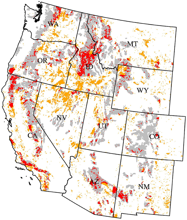
Figure 1. Study area spanning 11 states in the western USA. Areas spanned by MTBS burn polygons 1984–2018 are shown in red where they overlap USFS National Forest System (NFS) lands and in orange otherwise; unburned NFS lands are shown in gray.

At the time this research was undertaken, FIA plot data were publicly available for measurements taken in 2018 back through the year of initial implementation (which varied by state). All FIA plots are assessed for condition (e.g., forested vs. non-forested) and the attributes measured on forested conditions permit computation of live tree density over a range of age and size classes (seedlings, saplings, and larger trees) for each of the 4 subplots comprising an FIA plot (see Bechtold and Patterson 2005). Such data also exist for some regionally intensified FIA plot grids and regional post-fire FIA plot remeasurement designs, but these were not included in the analysis as they have variable spatial and temporal measurement intensities. For various reasons (e.g., presence of seasonal water, hazardous field conditions), vegetation data are not available for every subplot; such subplots were necessarily excluded from the analysis dataset and not utilized in averaging tree densities to a plot level. However, NFI subplot condition mapping procedures permitted the incorporation of data from subplots that were only partially measurable. The numbers of measurements of (at least) partially-forested FIA plots by state and year are summarized in Supplementary Figure 1.

Domains

This research centers on estimating post-fire tree density in forested areas of the western US experiencing wildland fire events. Thus, domains were defined using 1984–2018 burn perimeters obtained from the MTBS program (Eidenshink et al., 2007), which maps all wildland fires ≥404 ha in the western US. Also, in order to facilitate a focus on forested areas, where maintaining or re-establishing forest cover is a management objective, domains were restricted to the intersection of MTBS burn perimeters and USFS National Forest System (NFS) lands (excluding grasslands or other non-forest land designations, see Figure 1). Burned areas outside of these lands and burned areas on non-forested lands more generally were not considered parts of the domains of interest. Finally, US state boundaries were overlaid over the burn perimeters. This was done in part to account for differential sampling intensities over time across states (see Supplementary Figure 1), as well as to allow for estimation at a state-level resolution.

Given these constraints, the most finely resolved domains considered here consist of a complex of NFS lands within an individual western US state that are spanned by MTBS perimeters of a specific burn year. But also considered are aggregates of these domains taken over different time spans. Thus, allowing for a 2-year burn period, a domain can consist of NFS lands within a western US state spanned by MTBS perimeters from a given biennium; a 10-year burn period allows for domains consisting of NFS lands within an individual state spanned by MTBS perimeters from a given decade. In these instances, only non-overlapping time spans are considered; that is, in the 10-year case, we consider decadal domain burn periods ranging from 1990–1999 to 2000–2009.

The parameters of interest for each domain are taken as the mean tree densities at specified post-burn intervals. That is, as λ(d, l) defined by Equation (1) with y(x, l) denoting tree density (numbers of trees per ha) at location x at a temporal lag of l years post-fire. Below we consider only lags of 2 years or greater owing to the fact that data on first year germinants are not collected on FIA plots.

Domain Estimation

The FIA sample is distributed across all lands, while the domains of interest here span only burned, forested lands under NFS ownership. Therefore, the full FIA sample was first subset to plots falling within MTBS perimeters and within the states shown in Figure 1. The geographic coordinates of these plots and the standard cluster configuration were then used to determine the burned status of subplots. Data for subplots outside the bounds of any MTBS perimeters dating back to 1984 were dropped; measurement data for all remaining subplots were tied to the most recent MTBS burn and an associated fire-measurement lag computed. FIA condition mapping procedures then enabled elimination of subplots or portions of subplots classified to non-forest conditions (e.g., rangeland condition). Notably, subsetting to forested subplot data did not eliminate any plot measurements from our analysis set, it changed only the subplot support of those FIA plot measurements spanning multiple conditions. Finally, subplot measurement data were associated with the domains described above or with none of those domains (e.g., because a subplot was not located on NFS lands); data from the same domain and having the same lag were then aggregated to the plot level. All geospatial operations were undertaken in R (R Core Team, 2021).

Sample sizes available for direct estimation n(d, l) were determined from the number of FIA plot measurements falling within the domain d of interest and at the lag l of interest. In this, and in the subsequent estimators, plot-level records were treated the same irrespective of potentially differing numbers of subplots (e.g., because some subplots were outside the domain of interest or measured at a different lag). Plot-level compilations of trees per ha (all size classes, all species) were used for direct estimation of λ(d, l) via estimator (Equation 2). This domain sample mean ȳ(d, l) is not an unbiased (or conditionally unbiased) estimator of λ(d, l) under the FIA design. For instance, consider a domain known to completely encompass 10 hexagons comprising a 10-year remeasurement panel (see Bechtold and Patterson 2005) as well as portions of neighboring hexagons. Then, conditioning on a domain sample size of 1 also means conditioning on the location of the singular plot measurement coming from within one of the 10 completely spanned hexagons (and not from any of the incompletely spanned hexagons), meaning that the domain sample mean cannot be conditionally unbiased in general. Still, as with other ratio-type estimators the bias will decrease with increasing sample size. As an aside, we note that the domain sample mean (Equation 2) differs from the ratio estimation approach adopted by the FIA program. In this application, a y_k in Equation (2) is the number of trees on burned, partially-forested subplots of an FIA plot divided by the aggregate area of those burned, partially-forested subplots. The strategy advanced by Bechtold and Patterson (2005) is to instead (i) average the numbers of trees on burned forest land per unit plot area; (ii) average the areas of burned forest land per unit plot area; (iii) form a ratio of these two averages. Williams (2001) describes some of the key differences between these ratio estimators.

The standard error of ȳ(d, l) was estimated using

$\begin{array}{ll}\text{SE}\left[ȳ(d,l)\right]=\frac{{\widehat{\sigma }}_y(d,l)}{\sqrt{n(d,l)}}& (6)\end{array}$

where

$\begin{array}{ll}{\widehat{\sigma }}_y^2(d,l)=\frac{1}{n(d,l)-1}{\displaystyle \sum _{k\in s(d,l)}}{\left[y_k-ȳ(d,l)\right]}^2& (7)\end{array}$

is an estimator of the within-domain sample variance.

Direct estimates of λ(d, l) [where n(d, l) ≥ 1] and associated standard errors [where n(d, l) ≥ 2] were computed for all domains and all feasible lags. Tree density could not be estimated for all possible lags on all domains, however, because the annualized FIA program began only in 2001 (and only then for some states; see Supplementary Figure 1). Also, at the time of this research measurements were available only through 2018. Thus, for example, mean tree densities at the 5- and 10-year lags are estimable for the domain defined as NFS lands burned in California in 2000, but only at the 5-year lag for the domain defined as NFS lands burned in California in 2010. Variability in the numbers of domains for which tree density can be estimated by burn period and lag is summarized in Supplementary Figure 2 for domains of various burn interval lengths. It's also worth noting that for multi-year domains, lag remains constant and the applicable plot measurement years vary over the MTBS perimeters. For example in the case of the domain d comprised of NFS lands in ID burned in 2006 or 2007, the direct estimator of λ(d, l) for l = 10 uses only 2016 plot measurements for areas burned in 2006 fires and only 2017 measurements over the 2007 burns. This preserves the length of time elapsed between burns and corresponding plot observations.

Every direct domain and lag estimate was compared against two types of indirect estimates. The first type augmented the domain sample size by borrowing data from a broader spatial extent. Specifically, for a given domain d and lag l, all FIA plot measurements with the same lag l and falling within MTBS perimeters intersected by a spatial buffer extended around domain ${A}(d,l)$ were drawn into $\tilde{s}(d,l)$. Buffer distances ranging from 25 to 250 km were implemented in R (R Core Team, 2021). Note that under this procedure the augmented sample $\tilde{s}(d,l)$ can include plot data that are not within any domain of interest (i.e., in MTBS perimeters but outside the administrative state and/or NFS delineation), but only if the plot measurements were taken l years post-fire.

The second type of indirect estimate was obtained from augmented samples formed by borrowing data from a broader temporal extent. For a given domain d and lag l of interest, any FIA plot measurements made within the spatial extent ${A}(d,l)$ and at l ± δ years post-fire were drawn into $\tilde{s}(d,l)$. With this approach the augmented sample $\tilde{s}(d,l)$ can include only plot data from the same domain of interest [same MTBS perimeter(s)] but measurements taken prior or subsequently to the lag of interest. Thus, for a domain d defined as all 2010 MTBS burns on NFS lands in Montana and a lag of interest of l = 5 years, s(d, l) would consist only of plot data measured in 2015 within ${A}(d,5)$; but $\tilde{s}(d,l)$ would consist also of plot data measured in 2015 ± δ within the spatial extent ${A}(d,5)$ (provided 2015 − δ ≥ 2012 because only l≥2 year data are considered, and provided 2015 + δ ≤ 2018 because FIA measurements from 2019 or later were not available). Lag buffers δ ranging from 1 to 7 years were evaluated.

With both sample augmentation strategies, the indirect estimator (Equation 3) was applied. Furthermore, estimates of standard error were obtained similarly to direct estimation as

$\begin{array}{ll}\widehat{\text{SE}}\left[\widehat{ȳ}(d,l)\right]=\frac{{\widehat{\widehat{\sigma }}}_y(d,l)}{\sqrt{ñ(d,l)}}& (8)\end{array}$

where

$\begin{array}{ll}{\widehat{\widehat{\sigma }}}_y^2(d,l)=\frac{1}{ñ(d,l)-1}{\displaystyle \sum _{k\in \tilde{s}(d,l)}}{\left[y_k-\widehat{ȳ}(d,l)\right]}^2& (9)\end{array}$

Thus, the estimated standard error for the indirect estimator is a function of both a potentially larger sample size and of the variability within that larger sample. Relative standard error was obtained by relating $\widehat{\text{SE}}$ to estimated tree density.

MSE Estimation

Equation (8) can be used to estimate the precision of the indirect estimator, but makes no attempt to account for its inherent bias; a useful indicator of this estimator's accuracy would account for both. Equation (4) led to two estimators of the MSE of the indirect domain estimators (see Appendix B for details). The simplest, again suppressing the domain and lag indices d and l for brevity, takes the form

$\begin{array}{ll}\widehat{\text{MSE}}{\left[\widehat{ȳ}\right]}_1={(\widehat{ȳ}-ȳ)}^2-\frac{{\widehat{\sigma }}_y^2}{n}& (10)\end{array}$

This MSE estimator is based on an approximation suggested by Rao and Molina (2015, p. 44) but employs ȳ in place of a strictly unbiased domain estimator. It does not attempt to account for the covariance between the direct and indirect domain estimators. As such, it can be expected to be more appropriate in contexts where augmented sample sizes are consistently much larger than domain sample sizes. The other estimator evaluated here takes the form

$\begin{array}{ll}\widehat{\text{MSE}}{\left[\widehat{ȳ}\right]}_2={\left(\widehat{ȳ}-ȳ\right)}^2-\frac{{\widehat{\sigma }}_y^2}{n}\left[1-2\frac{n}{ñ}\right]& (11)\end{array}$

In this estimator the factor $\left[1-2\frac{n}{ñ}\right]$ results from the inclusion of an estimated covariance between $\widehat{ȳ}$ and ȳ. We note that $\widehat{\text{MSE}}{\left[\widehat{ȳ}\right]}_2\ge \widehat{\text{MSE}}{\left[\widehat{ȳ}\right]}_1$ (though neither estimator is guaranteed to be positive) and expect that $\widehat{\text{MSE}}{\left[\widehat{ȳ}\right]}_2$ will be more accurate when augmented samples are not substantially larger than the corresponding domain samples. Finally, as suggested by Marker (1995) we computed estimated squared bias as of the indirect domain estimator as

$\begin{array}{ll}\hat{\text{K}}\left[\widehat{ȳ}\right]=\widehat{\text{MSE}}{\left[\widehat{ȳ}\right]}_q-{\widehat{\widehat{\sigma }}}_y^2(d,l)& (12)\end{array}$

for q = 1, 2.

Estimates of MSE and squared bias were computed for each domain and lag individually, and also averaged over groups of proximate domains. The latter strategy was suggested by Gonzalez and Waksberg (1973) to reduce instability in MSE or squared bias estimates. In this study, we averaged MSE and squared bias estimates over all domains within the same state and having the same burn period length (e.g., any biennium for domains with 2-year burn periods), as well as over all estimation lags.

Results

Over the 11 states of the western USA shown in Figure 1, there were 4,778 FIA P2 plot locations falling at least partially within MTBS burn perimeters dating from 1984 to 2018. These locations provided 5,946 plot measurements from burned areas with measurement lags ranging from 2 to 35 years post-fire.

The distribution of domain sample sizes for domains of different temporal extents is shown in Figure 2. For domains spanning only a single burn year (e.g., all NFS lands burned in OR in 2000), sample sizes are almost so small as to prohibit direct estimation: in only 6% of cases (domains × lags) did the sample size exceed 5 observations. Even for domains spanning 4-years (e.g., all NFS lands burned in OR between 2000 and 2003), the median sample size is only 2 observations. This rises to 7 in the case of decadal domains (e.g., all NFS lands burned in OR between 2000–2009), the lowest temporal resolution considered to be of administrative utility.

FIGURE 2

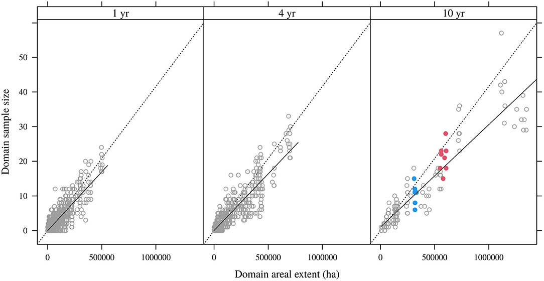
Figure 2. Domain sample sizes and areas for annual, quadrennial, and decadal domains, showing data for all lags. Dotted line is the nominal FIA sampling intensity; solid lines are linear regressions for particular lag buffers. Red symbols denote various lags for the OR 2000–2009 domain; blue symbols denote estimable lags for the ID 1990–1999 domain.

Though small, and inherently random, these domain sample sizes are governed in part by the FIA sampling intensity of approximately 1 plot measurement per 2,400 ha per decade. That nominal intensity is shown as the dotted line in Figure 2; realized intensities are captured by the solid lines that consistently fall short of the approximately 1:24,000 nominal rate.

Figure 2 also highlights two distinct domains for reference. Shown in red is the domain comprising OR NFS lands burned between 2000 and 2009 (lags 2–9 year). At lag 2 year, this domain spanned an areal extent of 605,690 ha, but with partial reburns the extent dropped to 550,806 ha at lag 9 year. Sample sizes ranged from 15 (lag 6 year) to 28 (lag 4 year), reflecting the generally high inter-annual variation in domain sample sizes. In blue is the domain comprising ID NFS lands burned between 1990 and 1999 (lags 14–19 years). This domain spanned an area of 332,272 ha at lag 14 year and captured sample sizes ranging from 6 to 15 observations.

Restricting attention to decadal domains, the relationship between area and estimated standard error of the domain sample means is shown in Figure 3. Domains with larger areal extents generally had larger sizes (see Figure 2) and smaller standard errors (Figure 3, left panel), though there is substantial variation around the latter trend. Moreover, standard errors could not even be computed for 15% of cases owing to domain sample sizes less than 2; over the remaining cases the median relative standard error was 47%. Figure 3 also shows the relationship between estimated standard errors (where these could be computed) and domain sample means. On the natural logarithm scale, there is a strong linear association between the domain sample mean and its estimate standard error.

FIGURE 3

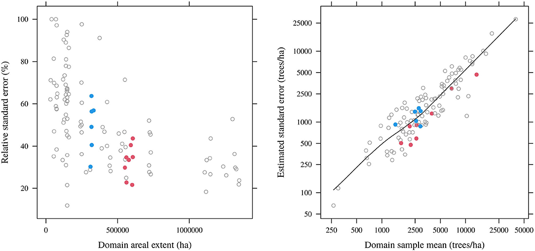
Figure 3. Relationships between estimated relative standard errors of domain sample means and domain areas (left) and between estimated standard errors and domain sample means (right; log scale). Only results for 10-year domains (any lags) and domain sample sizes above 2 are shown.

Borrowing data from an extended spatial extent generally augments the sample sizes available for indirect domain estimation (Figure 4). The dotted lines in Figure 4 correspond to the same nominal sampling intensity as in Figure 4, while the solid lines now show the realized augmented sampling intensities. As expected, the larger the spatial buffer and the larger the initial domain extent, the greater the increase in sample size. However, the spatial buffering operation yields erratic results at the domain level. For the domain spanning OR NFS lands burned between 2000 and 2009 (red symbols), spatial buffering greatly and consistently increases the sample sizes available for estimation. Yet the effect is much less pronounced for the domain spanning ID NFS lands burned between 1990 and 1999.

FIGURE 4

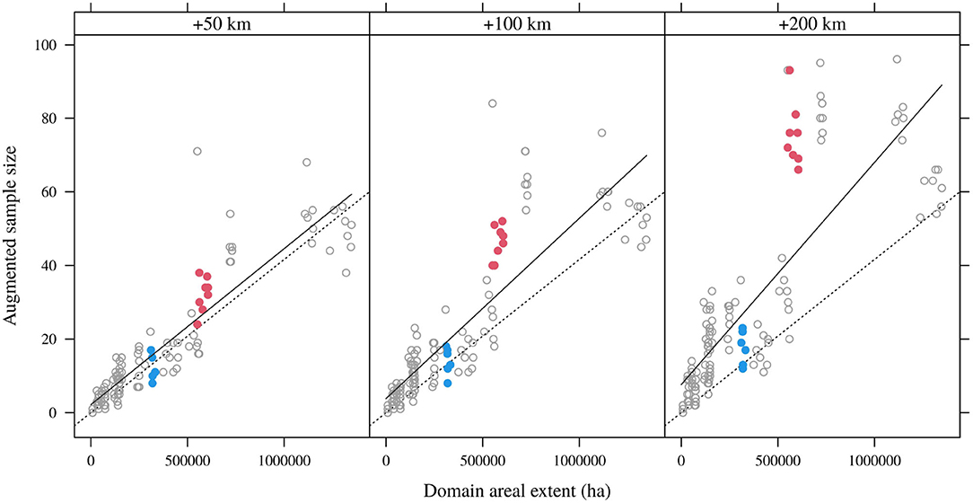
Figure 4. Augmented sample sizes and domain areas for 10-year domains (all lags) and different spatial buffers (50, 100, and 200 km). Dotted line is the nominal FIA sampling intensity; solid lines are linear regressions for particular spatial buffers.

The distribution of estimated standard errors for indirect estimates borrowing proximate spatial data, relative to those for direct estimates, is shown in Figure 5 for 10-year domains. Although the relative standard errors of indirect estimates are larger than those for the corresponding direct estimates in some cases (even with 200 km buffers), spatially augmented samples tend to reduce relative standard errors. The extent of the shift in the distribution of standard errors is a function of the magnitude of the spatial buffer, as expected. However, the magnitude of the shift is not pronounced and the median relative standard error using a 200 km buffer is still 38%. In addition, even at a 200 km buffer, 5% of cases (10-year domains × estimable lags) have augmented sample sizes less than 2 and thus do not permit estimation of standard errors.

FIGURE 5

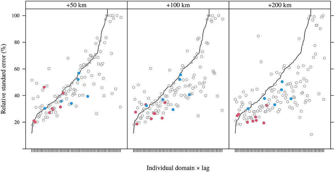
Figure 5. Estimated relative standard errors of augmented sample means for 10-year domains (all lags) under for different spatial buffers; domains and lags are ordered according to relative standard errors of domain means (as represented by the black curve). Horizontal axis labels are individual domain and lag identities and have been suppressed for clarity.

Relative to spatial buffering, borrowing data from an expanded temporal extent augments domain sample sizes at a consistent rate (Figure 6). The dashed lines in Figure 6 represent the nominal sampling intensity of a domain augmented according to the expanded temporal range of measurements. Specifically, one would expect approximately 1 FIA plot measurement at a given lag l within a domain of 24,000 ha; by extension, in allowing for plot measurement lags of l ± δ one would expect to collect 1 + 2δ plot measurements for a domain of that size. Mean augmented sample sizes (solid lines in Figure 6) fall short of the expected augmented sample sizes, but the sample augmentation effect is more consistent across domains than with spatial buffering. That is, with an expanded temporal extent there is less variability in the proportionate increases in sample sizes across domains, as indicated for the highlighted OR and ID domains.

FIGURE 6

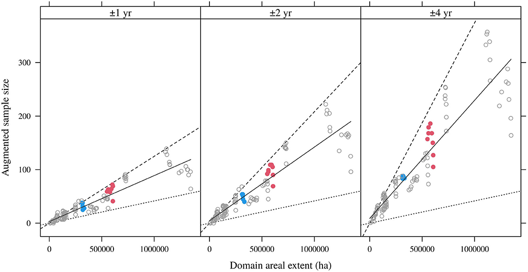
Figure 6. Augmented sample sizes and domain areas for 10-year domains (all lags) and different lag buffers (δ = 1, 2, 4 year). Dotted line is the nominal FIA sampling intensity r ≈ 1:24, 000; dashed lines are augmented intensities (2δ + 1)r; solid lines are linear regressions for particular burn intervals.

Corresponding to the more consistent sample augmentation of temporal buffering, the impacts on the distribution of estimated standard errors of indirect estimates were larger and more consistent (Figure 7). Comparison to Figure 5 also shows that relative standard errors of indirect estimates under l ± δ borrowing are generally lower than under space borrowing. At the least intensive lag-borrowing level (δ = 1 yr), they exceed the corresponding standard errors of the direct estimator much less frequently than under space borrowing, at even the largest buffer distance (200 km). Also, unlike under space borrowing (Figure 5). Figure 7 shows substantial reductions in relative standard errors of both domains represented by red and blue points, which consistently decline with increasing δ until they are approximately equal across lags for both domains at δ = 4 yr.

FIGURE 7

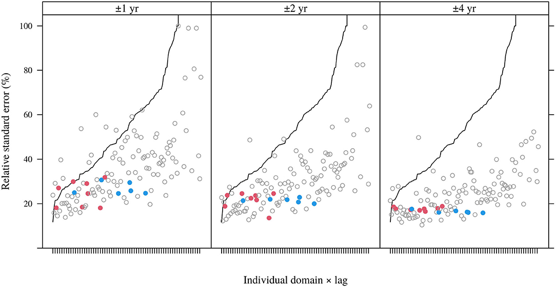
Figure 7. Estimated relative standard errors of augmented sample means for 10-year domains (all lags) under for different temporal buffers; domains and lags are ordered according to relative standard errors of domain means (represented by the black curve). Horizontal axis labels are individual domain and lag identities and have been suppressed for clarity.

Turning to MSE and bias estimation, for the decadal domains considered above MSE of the indirect estimators couldn't be estimated in 14% of cases (19 of 132 domains × lag combinations) regardless of temporal or spatial buffers employed. This was a result of domain sample sizes less than 2, which precluded estimation of ${\widehat{\sigma }}^2(d,l)$ and thus of $\widehat{\text{MSE}}{\left[\widehat{ȳ}\right]}_1$ or $\widehat{\text{MSE}}{\left[\widehat{ȳ}\right]}_2$. Even setting aside such cases, both MSE estimators frequently produced negative estimates when applied at the domain level. For example, for the indirect estimates employing data with a lag buffer of δ = 1 year, $\widehat{\text{MSE}}{\left[\widehat{ȳ}\right]}_2$ was negative in 41% of cases (domains × lags) while $\widehat{\text{MSE}}{\left[\widehat{ȳ}\right]}_1$ was negative in 71% of cases. As δ increased, the frequency of negative $\widehat{\text{MSE}}{\left[\widehat{ȳ}\right]}_1$ declined (though never fell below 50%), but the frequencies of negative $\widehat{\text{MSE}}{\left[\widehat{ȳ}\right]}_2$ increased to converge with those of $\widehat{\text{MSE}}{\left[\widehat{ȳ}\right]}_1$. Figure 8 shows estimated relative MSE (%) for the indirect domain estimator with δ = 2 year plotted against domain area (ha), computed individually for each 10 year domain × lag combination, using Equation (11). While variability declined with domain area, it is clear that both MSE estimators are too variable across domains and within domains across lags to be of operational utility at the domain level.

FIGURE 8

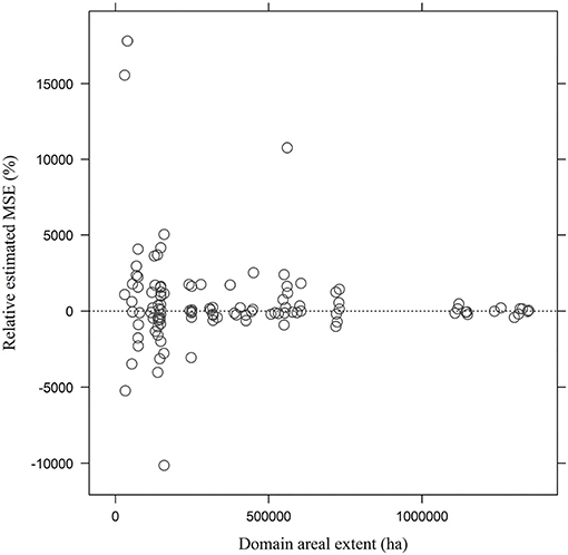
Figure 8. Estimated relative MSE (%) for the indirect domain estimator with δ = 2 plotted against domain area (ha), computed individually for each 10 year domain × lag combination using Equation (11).

Furthermore, both MSE estimators were still negative when averaged over proximate domains. Specifically, across different temporal buffers δ, $\widehat{\text{MSE}}{\left[\widehat{ȳ}\right]}_2$ yielded negative estimates for 20–40% of groups and $\widehat{\text{MSE}}{\left[\widehat{ȳ}\right]}_1$ for 50–90% of groups. Squared bias as estimated by Equation (12), which subtracts the variance of the indirect estimator from a corresponding MSE estimate, was necessarily negative even more often than either MSE estimator taken alone.

Discussion

The framework for indirect domain estimation we propose could be generalized to any probability sample of a target forest attribute (e.g., mean forest biomass density, total merchantable timber volume) distributed across spatiotemporal domains. Domains may span any time periods (for which requisite inventory data are available) and be comprised of contiguous or disjoint spatial polygons. It's worth remarking on the inherently complex nature of spatiotemporal domains comprised of burn perimeters intersecting a specific ownership category. Polygons are disjoint, often intersecting (reburns), and irregularly distributed in time and space according to neighborhood fire legacies.

When we expand domain delineations in space or time, the number of FIA P2 plot measurements will increase at a pace just below the nominal rate of approximately 1 measurement per 24,000 additional hectare-years (Figure 2). As we expand domains, however, they gradually lose administrative utility. For example, estimates of post-fire regeneration in areas burned over a reasonably narrow burn period length but extending over a vast geographic region (e.g., multiple states), or alternatively over a reasonably small geographic area but extending between 1984 and 2004 (20-year burn year window), would provide information of little utility to managers trying to optimize limited post-fire management resources for maximal regeneration impact.

Domain samples fluctuate around their anticipated sizes (given the nominal FIA sampling intensity and domain areas) owing in part to how the stratified random spatial distribution of plots intersects historic burn patterns. However, that the relationship between realized domain sample sizes and areas consistently falls short of its expectation must be due in large part to the fact that tree data are available only for FIA plots that are classified as partially forested. It may also be due in part to a tendency to fall short of annual plot remeasurement targets (see e.g., Roesch 2018). It is important to note that the consistent 1 observation per additional 24,000 ha⁻¹ yr⁻¹ burned area sample augmentation rate can only be expected to reliably emerge in years following the implementation of FIA's annualized inventory measurement protocols. This wasn't until 2001 at the earliest, 2011 in Wyoming, and with irregularities due to inconsistencies in funding in the interim (Supplementary Figure 1).

Our analysis of domain and augmented sample sizes and associated standard errors showed 10-year state-level domains to be the smallest spatiotemporal domains of administrative or management utility feasible for estimation of post-fire forest density using the domain estimators evaluated. As a general approach to estimation, direct FIA-based domain expansion estimation is unfeasible due to insufficiently small domain sample sizes and resultant high domain-level standard errors, even in 10-year domains. We note as well that we didn't account for the effects of retained plot size (e.g., only burned subplots) as implemented here on variance estimates. Hill et al. (2018) describe a methodology for incorporating differential plot sizes. Finally, though it wasn't an objective of this research, experimentation with other means of estimating the variance of domain estimates may be warranted (e.g., through the use of generalized variance functions as described by Wolter 2007, Chapter 7). A strong relationship between direct domain tree density estimates and their relative standard errors (Figure 3, right panel) was observed, as has been noted in other studies (e.g., Breidenbach et al. 2018).

Indirect estimators may offer an alternative. They are attractive in their potential to decrease domain-level standard errors. However, they rely on an implicit model that has the density of the attribute of interest changing slowly beyond the domain, at least relative to the variance of the attribute. We considered two strategies for borrowing data to augment domain samples for indirect estimation: borrowing in time (lag borrowing) and borrowing in space (space borrowing).

Under space borrowing, the rate of increase of the augmented sample size is dependent on the neighborhood fire legacy, the neighborhood land use patterns, and the overall sampling intensity. If many nearby forested hectares burned in the time range of interest, the augmented sample size will increase more quickly when data are drawn from a region only slightly expanded in space. Conversely, in areas with lower levels of nearby historic fire activity or lower levels of nearby forest land, one would need to expand further in space to obtain comparable increases in sample size. Yet borrowing extra-domain sample data in this way necessarily introduces bias to domain estimates. As plot observations from further away are selected for inclusion in the augmented domain sample, the biotic and abiotic environmental conditions of disparate forests may resemble those of the focal domain to a lesser extent. For example, borrowing in space can (and was observed to) draw on plot observations from distinct ecological conditions.

Another means of borrowing data that are proximate in space is to restrict the augmented sample to measurements (with appropriate postfire lag) from the same or similar ecological domains, regions or subsections (e.g., as delineated by Cleland et al. 1997). Nationwide availability of ecoregion designations of varied resolution would permit such restrictions. The capacity to augment the domain sample at a consistent rate, however, would still be governed by regional fire perimeter distributions in time and space. It would also then be impacted by regional landscape heterogeneity as exemplified by, for instance, varied ecoregions in mountainous terrain (with distinct forest and wildfire fuel type changes occurring over relatively short distances). An alternative approach wherein the augmented sample sizes could be fixed would be to borrow from the ideas underlying coarsened exact matching (see e.g., Van Deusen and Roesch 2013). That is, an initial spatial and/or ecological buffer could be evaluated and then, for domains still having an insufficient augmented sample size, the spatial buffer could be extended or the ecological classification coarsened. More generally, drawing data from outside the domain of interest but from regions that share other characteristics (e.g., ecological subsection) has parallels in the ideas underlying post-stratification. Yet post-stratified estimation is most commonly implemented as a strictly direct estimation approach (e.g., Haakana et al. 2020) without drawing on data from strata that extend beyond the domain of interest.

The spatial buffering algorithm utilized here can also be related to nearest neighbor techniques (e.g., McRoberts 2012) in that both define a neighborhood from which to borrow data. However, nearest neighbor techniques select a fixed number of observations using a neighborhood defined in a broader auxiliary space (typically not restricted to or even dependent on geographic variables), while under space borrowing the number of observations selected into the augmented sample is a random function of neighborhood fire legacy. For domains where few additional observations are obtained under space borrowing even with large buffer distances, nearest neighbor techniques may need to reach very far in geographic space to obtain the specified fixed number of neighbors, with the potential to increase estimation bias.

Adoption of the temporal buffering algorithm allows for the use of plot observations from the same geographic extent as the domain of interest but measured at differing lengths of time-since-disturbance. Though data from additional plot locations falling within that extent are introduced, this method borrows only in time. Other SAE applications in forest inventory have pooled data from multiple years to generate domain estimates for domains with fixed spatial extents and (usually implicit) multi-year temporal extents (e.g., Breidenbach and Astrup, 2012; McRoberts, 2012; Hill et al., 2018). Here, we explicitly borrow sample observations with measurement years other than those denoted by the spatiotemporal domain parameters and target estimation lag. Spatiotemporal disturbance domains require a high degree of specificity in domain definition, and by extension in the definition of the temporal component of the target attribute. This specificity led to the determination that to include observations with measurement years other than those specified by the relevant disturbance lag is to operate in the realm of indirect estimation. Thus, the general estimation strategy employed by Breidenbach and Astrup (2012) that integrates data measured between 2005 and 2010 to estimate a periodic mean is distinct from our lag-borrowing indirect estimation strategy. With δ = 2 year, the latter would draw on observations from 2005 to 2009 to indirectly estimate a target attribute in 2007, but on observations from 2006 to 2010 to indirectly estimate a target attribute in 2008.

Even in areas exhibiting highly unfavorable conditions for post-fire forest regeneration, some seeds will germinate, some seedlings will establish, and some patches of forest will eventually begin to regenerate over time. Thus, to include plots with measurement years earlier than specified by d and l in $\tilde{s}(d,l)$ is to include observations which may not capture the full extent of forest stand development in the focal domain, leading to negative bias. Conversely, to include plots with later measurement years is to include observations which may exaggerate the extent of true forest stand development in the focal domain, leading to positive bias.

As implemented in this study, lag borrowing augmented domain samples (Figure 6) and decreased relative domain standard errors (Figure 7) to a greater extent, and in a faster, more consistent manner, than space borrowing (Figures 4, 5). The smaller increases in precision of the indirect estimator achieved via space borrowing relative to lag borrowing largely reflect instances where few additional plots were obtained by space borrowing (e.g., as in the case of the domain represented by blue points in Figure 4). This could also result from instances where plots from adjacent ecoregions with markedly different regeneration conditions were selected, adding to within-sample variability. Space borrowing has been shown to be effective in domains whose spatiotemporal neighborhoods yield more observations available for sample augmentation, for instance the estimation of an attribute over a single time period distributed across most or all adjacent forested area (e.g., Breidenbach and Astrup, 2012; Magnussen et al., 2014a).

As methods for borrowing increase in complexity, so do their associated sources, and likely magnitudes, of bias. For this reason we evaluated explicit space and lag borrowing only. Overall, lag borrowing exhibited greater magnitude and consistency of increases in both augmented samples and precision of estimates relative to space borrowing. These facts combine to suggest lag borrowing to be a superior borrowing strategy to space-borrowing for indirect expansion estimation of post-fire tree density in western US-wide spatiotemporal domains with respect to domain-level standard errors. That said, estimation of the bias of indirect domain estimators remains a challenge. An obstacle in formulating estimators of the MSE or squared bias of an indirect domain estimator from Equations (4) to (5) is the difficultly of reliably estimating the variance of an unbiased domain estimator—for the absence of a precise direct estimator is generally what motivates indirect estimation in the first place. The MSE estimators proposed by Rao and Molina (2015) and Gonzalez and Waksberg (1973), and squared bias estimator proposed by Marker (1995), can be negative and yield widely disparate MSE estimates for a single domain at lags separated by just one or several years, as occurred in our application. This resulted from subtraction of the unstable and often large estimated variance of the direct domain estimator.

The MSE estimator we proposed, which accounts for the covariance between direct and indirect domain estimates, constituted some improvement but was still unstable and frequently negative (Figure 8). It was also very high in some domains, and in fact is necessarily larger than the other estimator investigated. As suggested by Gonzalez and Waksberg (1973) and Rao and Molina (2015), we also averaged $\widehat{\text{MSE}}{\left[\widehat{ȳ}\right]}_1$ and $\widehat{\text{MSE}}{\left[\widehat{ȳ}\right]}_2$ over proximate domains to improve stability, but this yielded only marginal improvements.

Indirect FIA-based expansion estimation of post-fire tree regeneration in US state-level domains is probably most feasible in domains with burn year periods of 10 years, owing to small augmented sample sizes in many domains of shorter burn period lengths. By δ = 2 yr, the vast majority of standard errors of indirect lag-borrowed estimates are substantially lower than their direct counterparts (Figure 7), suggesting δ = 2 or 3 as a potential starting point for operational domain estimation. This is with the understanding that we were unable to effectively characterize the bias of indirect estimates. Composite estimators (Rao and Molina, 2015) seek to balance the instability of an unbiased (or approximately unbiased) direct estimator with the bias of a more precise indirect estimator. Weights controlling the relative contributions of the component estimators are typically constructed using either domain sample sizes or their relative MSEs. Owing to our unreliable estimates of the MSE of the indirect estimator, we could not have constructed a composite estimator based on MSE. Though we could have devised weights using domain sample sizes, we did not expect the resultant composite estimates to be more precise than the indirect estimates based on lag borrowing alone, and in any case did not expect MSE estimation techniques to apply successfully to the composite estimator for the same reasons discussed above. These results point to the need for exploration of model-assisted or model-based SAE strategies that could draw on systematic associations (or effective post-stratifications) of postfire tree density as a function of auxiliary variables available across the population.

Conclusion

Direct FIA-based estimation of postfire tree density at particular times-since-disturbance is deemed unfeasible due to insufficiently small domain sample sizes. Indirect domain ratio estimators that borrow sample observations from outside a focal domain are alternatives to auxiliary-assisted methods and have the potential to consistently and rapidly augment decrease domain level standard errors. Borrowing in time proved to augment domain samples more consistently than borrowing in space. On the basis of relative standard errors alone, indirect estimation of postfire tree regeneration in 10-year state-level domains with δ = 2 or 3 presents a promising alternative to direct estimation.

As indirect estimators necessarily add bias to domain estimates, reliable estimators of MSE are required. MSE estimators of indirect domain estimators have been proposed and evaluated in the literature, and we evaluate a new MSE estimator that accounts for the covariance between direct and synthetic domain estimates. However, none of the MSE estimators evaluated performed adequately.

Our results highlight the difficulties of estimating MSE and squared bias, and point to the need for further experimentation with methods for estimating MSE, including potentially modeling MSE using appropriate covariates. Alternatively, unbiased SAE techniques that preclude the need for bias estimation, and that leverage auxiliary data, warrant inquiry in this context.

Data Availability Statement

True FIA plot center locations are confidential. Requests to access these datasets should be directed to https://www.fia.fs.fed.us/.

Author Contributions

GG and DA made major contributions to research and analysis. Both authors contributed to the article and approved the submitted version.

Conflict of Interest

The authors declare that the research was conducted in the absence of any commercial or financial relationships that could be construed as a potential conflict of interest.

Publisher's Note

All claims expressed in this article are solely those of the authors and do not necessarily represent those of their affiliated organizations, or those of the publisher, the editors and the reviewers. Any product that may be evaluated in this article, or claim that may be made by its manufacturer, is not guaranteed or endorsed by the publisher.

Acknowledgments

The availability of geospatial data used in this publication was made possible, in part, by an agreement from the United States Department of Agriculture's Forest Service (USFS). This publication may not necessarily express the views or opinions of the USFS. Support for this research was also provided by the Inland Northwest Growth & Yield Cooperative and by the USFS Rocky Mountain Research Station (20-JV-11221636-110).

Supplementary Material

The Supplementary Material for this article can be found online at: https://www.frontiersin.org/articles/10.3389/ffgc.2021.761509/full#supplementary-material

References

Baffetta, F., Fattorini, L., Franceschi, S., and Corona, P. (2009). Design-based approach to k-nearest neighbours technique for coupling field and remotely sensed data in forest surveys. Remote Sens. Environ. 113, 463–475. doi: 10.1016/j.rse.2008.06.014

CrossRef Full Text | Google Scholar

Bechtold, W. A., and Patterson, P. L. (2005). The Enhanced Forest Inventory and Analysis Program-National Sampling Design and Estimation Procedures. General Technical Report GTR-SRS-80, USDA Forest Service, Southern Research Station.

Google Scholar

Breidenbach, J., and Astrup, R. (2012). Small area estimation of forest attributes in the Norwegian national forest inventory. Eur. J. For. Res. 131, 1255–1267. doi: 10.1007/s10342-012-0596-7

CrossRef Full Text | Google Scholar

Breidenbach, J., Magnussen, S., Rahlf, J., and Astrup, R. (2018). Unit-level and area-level small area estimation under heteroscedasticity using digital aerial photogrammetry data. Remote Sens. Environ. 212, 199–211. doi: 10.1016/j.rse.2018.04.028

CrossRef Full Text | Google Scholar

Cleland, D. T., Avers, P. E., McNab, W. H., Jensen, M. E., Bailey, R. G., King, T., et al. (1997). National hierarchical framework of ecological units. Ecosyst. Manage. Appl. Sustain. For. Wildlife Resour. 20, 181–200.

PubMed Abstract | Google Scholar

Cordy, C. B. (1993). An extension of the Horvitz-Thompson theorem to point sampling from a continuous universe. Statist. Probability Lett. 18, 353–362.

Google Scholar

Coulston, J. W., Green, P. C., Radtke, P. J., Prisley, S. P., Brooks, E. B., Thomas, V. A., et al. (2021). Enhancing the precision of broad-scale forestland removals estimates with small area estimation techniques. Forestry 94, 427–441. doi: 10.1093/forestry/cpaa045

CrossRef Full Text | Google Scholar

Datta, G. S., Kubokawa, T., Molina, I., and Rao, J. N. K. (2011). Estimation of mean squared error of model-based small area estimators. Test 20, 367–388. doi: 10.1007/s11749-010-0206-2

CrossRef Full Text | Google Scholar

Eidenshink, J., Schwind, B., Brewer, K., Zhu, Z., Quayle, B., and Howard, S. (2007). A project for monitoring trends in burn severity. Fire Ecol. 3, 3–21. doi: 10.4996/fireecology.0301003

CrossRef Full Text | Google Scholar

Frank, B., and Monleon, V. J. (2021). Comparison of variance estimators for systematic environmental sample surveys: considerations for post-stratified estimation. Forests 12:772. doi: 10.3390/f12060772

CrossRef Full Text | Google Scholar

Gonzalez, M. E., and Waksberg, J. (1973). “Estimation of the error of synthetic estimates,” in First Meeting of the International Association of Survey Statisticians (Vienna), 18–25.

Grafström, A., Schnell, S., Saarela, S., Hubbell, S. P., and Condit, R. (2017). The continuous population approach to forest inventories and use of information in the design. Environmetrics 28:e2480. doi: 10.1002/env.2480

CrossRef Full Text | Google Scholar

Gregoire, T. G. (1998). Design-based and model-based inference in survey sampling: appreciating the difference. Can. J. For. Res. 28, 1429–1447. doi: 10.1139/x98-166

CrossRef Full Text | Google Scholar

Haakana, H., Heikkinen, J., Katila, M., and Kangas, A. (2020). Precision of exogenous post-stratification in small-area estimation based on a continuous national forest inventory. Can. J. For. Res. 50, 359–370. doi: 10.1139/cjfr-2019-0139

CrossRef Full Text | Google Scholar

Higuera, P. E., and Abatzoglou, J. T. (2021). Record-setting climate enabled the extraordinary 2020 fire season in the western United States. Glob. Chang Biol. 27, 1–2. doi: 10.1111/gcb.15388

PubMed Abstract | CrossRef Full Text | Google Scholar

Hill, A., Mandallaz, D., and Langshausen, J. (2018). A double-sampling extension of the German national forest inventory for design-based small area estimation on forest district levels. Remote Sens. 10, 1052–1078. doi: 10.3390/rs10071052

CrossRef Full Text | Google Scholar

Magnussen, S., Mandallaz, D., Breidenbach, J., Lanz, A., and Ginzler, C. (2014a). National forest inventories in the service of small area estimation of stem volume. Can. J. For. Res. 44, 1079–1090. doi: 10.1139/cjfr-2013-0448

CrossRef Full Text | Google Scholar

Magnussen, S., Næsset, E., and Gobakken, T. (2014b). An estimator of variance for two-stage ratio regression estimators. For. Sci. 60, 663–676. doi: 10.5849/forsci.12-163

CrossRef Full Text | Google Scholar

Marker, D. A. (1995). Small Area Estimation: A Bayesian Perspective (Ph.D. thesis). University of Michigan.

Google Scholar

McRoberts, R. E. (2012). Estimating forest attribute parameters for small areas using nearest neighbors techniques. For. Ecol. Manage. 272, 3–12. doi: 10.1016/j.foreco.2011.06.039

CrossRef Full Text | Google Scholar

R Core Team (2021). R: A Language and Environment for Statistical Computing. Vienna: R Foundation for Statistical Computing.

Google Scholar

Rao, J. N. K., and Molina, I. (2015). Small Area Estimation, 2nd Edn. Hoboken, NJ: Wiley.

Google Scholar

Roesch, F. (2018). Composite estimators for growth derived from repeated plot measurements of positively-asymmetric interval lengths. Forests 9, 427. doi: 10.3390/f9070427

CrossRef Full Text | Google Scholar

Särndal, C.-E., Swensson, B., and Wretman, J. (2003). Model Assisted Survey Sampling. New York, NY: Springer Science & Business Media.

Google Scholar

Ståhl, G., Saarela, S., Schnell, S., Holm, S., Breidenbach, J., Healey, S. P., et al. (2016). Use of models in large-area forest surveys: comparing model-assisted, model-based and hybrid estimation. For. Ecosyst. 3, 1–11. doi: 10.1186/s40663-016-0064-9

CrossRef Full Text | Google Scholar

Stevens-Rumann, C. S., Kemp, K. B., Higuera, P. E., Harvey, B. J., Rother, M. T., Donato, D. C., et al. (2017). Evidence for declining forest resilience to wildfires under climate change. Ecol. Lett. 21, 243–252. doi: 10.1111/ele.12889

PubMed Abstract | CrossRef Full Text | Google Scholar

Van Deusen, P., and Roesch, F. (2013). Trends and projections from annual forest inventory plots and coarsened exact matching. Math. Comput. For. Natural Resour. Sci. 5, 126–134.

Google Scholar

Williams, M. S. (2001). Comparison of estimation techniques for a forest inventory in which double sampling for stratification is used. For. Sci. 47, 563–576. doi: 10.1093/forestscience/47.4.563

CrossRef Full Text | Google Scholar

Wolter, K. M. (2007). Introduction to Variance Estimation, 2nd Edn. Springer.

Google Scholar

Appendix

Appendix A: Mean & Variance of the Direct Estimator

Adopting the continuous population framework of Cordy (1993), we consider equal probability sampling designs that can be described by specifying a constant inclusion density function π(x, t) = π(t) for all possible measurements locations over a land surface in a given year t. For such designs, the direct domain estimator (2) can be formulated as a ratio of the two Horvitz-Thompson domain estimators

$\begin{array}{ll}{\widehat{\tau }}_{\pi }(d,l)={\displaystyle \sum _{k\in s(d,l)}}\frac{y_k}{\pi (l)}=\frac{{\displaystyle {\sum }_{k\in s(d,l)}}{y}_k}{\pi (l)}& (\mathrm{A1a})\end{array}$

$\begin{array}{ll}{Â}_{\pi }(d,l)={\displaystyle \sum _{k\in s(d,l)}}\frac{1}{\pi (l)}=\frac{n(d,l)}{\pi (l)}& (\mathrm{A1b})\end{array}$

where π(l) is the inclusion density function at l years following the defining disturbance event. Estimators (A1) are unbiased for the total of y over ${A}(d,l)$ at year l from disturbance, and for the total area of ${A}(d,l)$, respectively. Yet the nonlinear combination of these estimators is generally biased for λ(d, l). The domain sample mean (2) can be described as “approximately unbiased” in the sense that its bias diminishes with increasing expected n(d, l) (see Särndal et al., 2003, p. 185), though this is of limited utility in a small area estimation context where we anticipate small n(d, l).

Cordy (1993) provides a number of general results concerning the bias and variance of estimators such as ȳ(d, l). In particular, his results allow that if the conditional inclusion density function π_n(x, l) given n(d, l) is positive for all measurement locations within ${A}(d,l)$, then

$\begin{array}{ll}\text{E}\left[\overline{y}(d,l)|n(d,l)\right]=\lambda (d,l)& (\mathrm{A2})\end{array}$

provided n(d, l) > 0. This conditional unbiasedness result holds for SRS because under that design

$\begin{array}{ll}{\pi }_n(\text{x},l)=\frac{n(d,l)}{\left|{A}(d,l)\right|}& (\mathrm{A3})\end{array}$

for all $\text{x}\in {A}(d,l)$. However, conditional unbiasedness does not extend to all equal probability designs. For example, conditional on the hexagonal tessellation employed by the FIA's unaligned systematic design it is possible to have π_n(x, l) = 0 for some $\text{x}\in {A}(d,l)$ given n(d, l). In particular, suppose ${A}(d,l)$ spans one entire FIA phase 1 hexagon (see Bechtold and Patterson, 2005) slated for measurement in year l as well as portions of several other phase 1 hexagons; if n(d, l) = 1 then the conditional inclusion density function will be positive over the completely subsumed hexagon but must be 0 over the other intersected hexagons. This will generally result in bias. The above also assumes that y_k = y(x_k, l_k) is a point-measurement (or a measurement employing protocols suitably adjusted for boundary overlap) and that one can thus ignore any boundary overlap effects (see e.g., Gregoire, 1998).

The variance of ȳ(d, l) for random n(d, l) has no analytically tractable form as it is a function of the variability of both estimators in (A1). From Cordy (1993), under SRS the conditional variance of ȳ(d, l) given n(d, l) can be written in the familiar form

$\begin{array}{l}\text{V}\left[\overline{y}(d,l)|n(d,l)\right]=\frac{1}{n(d,l)|A(d,l)|}{\displaystyle \underset{{A}(d,l)}{\int }{\left[y(\text{x},l)-\lambda (d,l)\right]}^2}\\ \text{ d}x=\frac{{\sigma }_y^2(d,l)}{n(d,l)}& (\mathrm{A4})\end{array}$

Furthermore, that variance can be (conditionally) unbiasedly estimated using

$\begin{array}{ll}\hat{\text{V}}\left[ȳ(d,l)\right]=\frac{1}{n(d,l)\left[n(d,l)-1\right]}{\displaystyle \sum _{k\in s(d,l)}}{\left[y_k-ȳ(d,l)\right]}^2=\frac{{\widehat{\sigma }}_y^2(d,l)}{n(d,l)}& (\mathrm{A5})\end{array}$

For spatially structured designs such as the USFS FIA, the variance will be a function of more complex pairwise inclusion density functions (see Cordy, 1993). Moreover, it may not be possible to derive (conditionally) unbiased variance estimators because the pairwise inclusion density function can be 0 for sets of proximate locations. In such settings, estimator (A5) has been recommended as a conservative variance estimator in the sense that it is expected to overestimate variability in cases where the spatial design effectively reduces sampling error (e.g., Baffetta et al., 2009; see also Wolter, 2007, pp. 47–48). Alternatively, variance estimation strategies developed for systematic designs (e.g., Frank and Monleon, 2021) could be evaluated.

Appendix B: Mean, Variance, & MSE of the Indirect Estimator

Certain properties of the indirect domain estimator (3) follow directly from the results of Appendix A. These are extended below suppressing the parenthetical domain and lag dependence notation (d, l) unless necessary.

Under SRS the conditional expectation of $\widehat{ȳ}$ is a function of the distribution of y over the expanded spatiotemporal region $\tilde{{A}}=\tilde{{A}}(d,l)$, i.e.,

$\text{E}\left[\widehat{\overline{y}}|\tilde{n}\right]=\frac{1}{\left|\tilde{{A}}\right|}{\displaystyle \underset{\tilde{{A}}}{\int }y}(x,l)\text{d}x=\frac{\left|{A}\right|}{\left|\tilde{{A}}\right|}\lambda +\frac{\left|\tilde{{A}}\right|-\left|{A}\right|}{\left|\tilde{{A}}\right|}\stackrel{°}{\lambda }=\tilde{\lambda }$

where $\tilde{\lambda }$ is the density of y over $\tilde{{A}}$ and $\stackrel{°}{\lambda }$ is the density of y over only the extra-domain region supplying additional data. The conditional bias of (3) as an estimator of λ will therefore be a function of the extent to which the density of y over the “small area” ${A}$ differs from that over the “large area” $\tilde{{A}}$. Additionally, under SRS the conditional variance of $\widehat{ȳ}$ can be written as

$\text{V}\left[\widehat{\overline{y}}|\tilde{n}\right]=\frac{1}{\tilde{n}\left|\tilde{{A}}\right|}{\displaystyle \underset{\tilde{{A}}}{\int }{\left[y(x,l)-\tilde{\lambda }\right]}^2}\text{d}x=\frac{{\tilde{\sigma }}_y^2}{\tilde{n}}$

where ${\tilde{\sigma }}_y^2$ is the variance in y over $\tilde{{A}}$. This conditional variance can be unbiasedly estimated using

$\begin{array}{ll}\hat{\text{V}}\left[\widehat{ȳ}\right]=\frac{1}{ñ\left[ñ-1\right]}{\displaystyle \sum _{k\in \tilde{s}}}{\left[y_k-\widehat{ȳ}\right]}^2& (\mathrm{A6})\end{array}$

conditional on the realized sample size ñ. As for the direct sample mean (2) these results do not extend generally to other (equal or unequal probability) spatial designs, but equation (A6) can again be applied as a conservative estimator of variance.

To describe the MSE of $\widehat{ȳ}$, it is useful to note that it can be broken down much like its expectation above

$\begin{array}{ll}\widehat{ȳ}=\frac{1}{ñ}{\displaystyle \sum _{k\in \tilde{s}}}{y}_k=\frac{1}{ñ}\left({\displaystyle \sum _{k\in s}}{y}_k+{\displaystyle \sum _{\begin{array}{c}k\in \tilde{s}\\ k\notin s\end{array}}}{y}_k\right)=\frac{n}{ñ}ȳ+\frac{ñ-n}{ñ}\ddot{ȳ}& (\mathrm{A7})\end{array}$

where $\ddot{ȳ}=\ddot{ȳ}(d,t)$ is the mean of the observations in $\tilde{s}$ but not in s (i.e., of the observations that have been borrowed from outside the domain of interest). Then, adopting the approach used by Rao and Molina (2015, p. 43), write the conditional MSE of the indirect estimator (3) given n as

$\begin{array}{l}\text{MSE}\left[\widehat{\overline{y}}|n\right]n=\text{E}\left[{\left(\widehat{\overline{y}}-\overline{y}\right)}^2|n\right]+\text{E}\left[{\left(\overline{y}-\lambda \right)}^2|n\right]\\ +2\text{E}\left[\left(\widehat{\overline{y}}-\overline{y}\right)\left(\overline{y}-\lambda \right)|n\right]n\\ =\text{E}\left[{\left(\widehat{\overline{y}}-\overline{y}\right)}^2|n\right]+\text{E}\left[{\left(\overline{y}-\lambda \right)}^2|n\right]\\ -2\text{E}\left[\overline{y}\left(\overline{y}-\lambda \right)|n\right]+2\text{E}\left[\widehat{\overline{y}}\left(\overline{y}-\lambda \right)|n\right]& (\mathrm{A8})\end{array}$

The second and third terms on the right hand side of (A8) relate to the variability of ȳ(d, t) while the last term connects to the association between ȳ(d, t) and $\widehat{ȳ}(d,t)$. Indeed, under SRS, (A8) can be simplified to

$\begin{array}{ll}\text{MSE}\left[\widehat{\overline{y}}|n\right]=\text{E}\left[{\left(\widehat{\overline{y}}-\overline{y}\right)}^2|n\right]-\text{V}\left[\overline{y}|n\right]+2\text{C}\left[\widehat{\overline{y}},\overline{y}|n\right]& (\mathrm{A9})\end{array}$

where $\text{C}\left[\widehat{\overline{y}},\overline{y}|n\right]$ denotes (conditional) covariance. Further simplification is possible under SRS by focusing on the covariance term

$\begin{array}{l}\text{C}\left[\widehat{\overline{y}},\overline{y}|n\right]=\text{E}\left[\widehat{\overline{y}}\left(\overline{y}-\lambda \right)|n\right]\\ =\text{E}\left\{\text{E}\left[\widehat{\overline{y}}\left(\overline{y}-\lambda \right)|n,\tilde{n},s\right]|n\right\}\\ =\text{E}\left\{\left(\overline{y}-\lambda \right)\text{E}\left[\widehat{\overline{y}}|n,\tilde{n},s\right]|n\right\}& (\mathrm{A10})\end{array}$

Substituting (A7), the inner expectation of (A10) becomes

$\text{E}\left[\widehat{\overline{y}}|n,\tilde{n},s\right]=\frac{n}{\tilde{n}}\overline{y}+\frac{\tilde{n}-n}{\tilde{n}}\text{E}\left[\ddot{\overline{y}}|n,\tilde{n},s\right]=\frac{n}{\tilde{n}}\overline{y}+\frac{\tilde{n}-n}{\tilde{n}}\stackrel{°}{\lambda }$

Thus,

$\begin{array}{l}\text{C}\left[\widehat{\overline{y}},\overline{y}|n\right]=\text{E}\left\{\left(\overline{y}-\lambda \right)\frac{n}{\tilde{n}}\overline{y}+\left(\overline{y}-\lambda \right)\frac{\tilde{n}-n}{\tilde{n}}\stackrel{°}{\lambda }|n\right\}\\ =\text{E}\left\{\frac{n}{\tilde{n}}|n\right\}\text{E}\left\{\left(\overline{y}-\lambda \right)\overline{y}|n\right\}+\stackrel{°}{\lambda }\text{E}\left\{\frac{\tilde{n}-n}{\tilde{n}}\left(\overline{y}-\lambda \right)|n\right\}\\ =\text{E}\left\{\frac{n}{\tilde{n}}|n\right\}\text{V}\left[\overline{y}|n\right]\end{array}$

Finally, substituting this last result into (A9) gives

$\begin{array}{ll}\text{MSE}\left[\widehat{\overline{y}}|n\right]=\text{E}\left[{\left(\widehat{\overline{y}}-\overline{y}\right)}^2|n\right]-\text{V}\left[\overline{y}|n\right]\left[1-2\text{E}\left\{\frac{n}{\tilde{n}}|n\right\}\right]& (\mathrm{A11})\end{array}$

Note that if ñ = n so that no observations are borrowed and that therefore $\widehat{\overline{y}}=\overline{y}$, then $\text{MSE}\left[\widehat{\overline{y}}|n\right]$ collapses to simply V[ȳ|n], as it should. However, if data are drawn from a much larger area such that ñ≫n then $\text{MSE}\left[\widehat{\overline{y}}|n\right]$ tends to $\text{E}\left[{\left(\widehat{\overline{y}}-\overline{y}\right)}^2|n\right]-\text{V}\left[\overline{y}|n\right]$. The latter expression is suggested as an approximation by Rao and Molina (2015, p. 44), but will be too small unless data are drawn from a substantially larger area than the domain of interest. Finally, note again that this expression applies in the case of SRS, but not more generally.

Expression (A11) suggests a simple sample-based estimator of the conditional MSE

$\begin{array}{ll}\widehat{\text{MSE}}\left[\widehat{\overline{y}}|n\right]={\left(\widehat{\overline{y}}-\overline{y}\right)}^2-\frac{{\widehat{\sigma }}_y^2}{n}\left[1-2\frac{n}{\tilde{n}}\right]& (\mathrm{A12})\end{array}$

This estimator differs from the framework suggested by Rao and Molina (2015, p. 44) only by the factor $\left[1-2\frac{n}{ñ}\right]$; this factor guarantees larger estimates of MSE, but still cannot guarantee non-negative estimates. We are unaware of any investigation of its sampling properties, however.