GREGORY: A Modified Generalized Regression Estimator Approach to Estimating Forest Attributes in the Interior Western US

1. Introduction

The US Forest Inventory and Analysis Program (FIA) is responsible for monitoring forest ecosystems across the United States. Established in 1930, the initial focus of this program was to estimate the extent and volume of merchantable trees for harvest. But today the extensive data collected nationwide are valuable for assessing biomass and carbon storage, fuels and fire risk, wildlife habitat, effects of insect and disease outbreaks, forest health and trends in forest conditions. Along with these new uses, FIA is experiencing a greater demand for estimates of forest attributes over smaller geographic areas. Specifically, the “Agricultural Act of 2014” (U.S. Department of Agriculture, 2014) calls for FIA to implement procedures to improve precision in sub-state estimates, pushing the inventory to provide information at scales beyond which it was originally intended. Producing reliable estimates for these smaller areas requires considering additional data sources and new estimation methods beyond FIA's current techniques.

One standard estimation approach is the generalized regression estimator (GREG), which has the capacity of combining inventory data and remote-sensing data using a wide range of predictive modeling techniques (Särndal et al., 1992; Breidt and Opsomer, 2017). The GREG is a direct estimator, since it only uses data within the domain of interest and is design-based in that randomness comes solely from sample selection. The GREG is asymptotically unbiased, regardless of how well the model captures the true relationship between the inventory and auxiliary data. This useful feature is why the estimator is classified as model-assisted and not model-based.

Using a variety of assisting models, the GREG has been applied and studied rather extensively in the forest inventory literature (Baffetta et al., 2009; McRoberts, 2010; Gregoire et al., 2011; Moser et al., 2017; McConville et al., 2020). A thorough summary of forest inventory estimators that utilize models, including model-assisted estimators like the GREG, can be found in Ståhl et al. (2016). Most of the focus in these articles is on large areas with adequate sample sizes within the domain of interest. For areas with few sampled ground plots, the model estimates may not capture the true relationship well and may be highly variable. A solution is to leverage sample data outside the domain of interest to estimate the GREG's assisting model, resulting in what is sometimes referred to as a modified GREG (Rao and Molina, 2015). Most commonly the entire sample across all domains of interest is used to fit the model for the modified GREG. Here we consider estimating the models over large homogeneous regions and then combining the model predictions within the domain of interest. We call this estimator GREGORY for GREG Over Resolutions of Y, where Y stands for the inventory data, to emphasize that the additional regions leveraged should depend on their homogeneity with the inventory data in the domain of interest. Although the GREGORY leverages data from outside the domain of interest, Rao and Molina (2015) still classify it as a direct estimator, since it only applies model parameter estimates to the plot data within the domain of interest and is still design-based in that randomness comes solely from sample selection. As with the GREG, the GREGORY is model-assisted, an important feature to national statistical agencies.

While the modified GREG, or GREGORY, has been proposed in the survey statistics literature (section 2.5 in Woodruff, 1966; Rao and Molina, 2015), it does not, to the best of our knowledge, appear to have been investigated deeply in the forest inventory literature. In this article, we hope to provide some insights into the utility of the GREGORY for forest estimation. Through a case study focused on estimating county level means of forest attributes in the US Interior West (IW), we attempt to measure how the estimator precision changes when the model-estimating now leverages additional data outside the domain of interest. Additionally, we investigate how precision gains from estimating the model over these broader samples change and the bias of the standard variance estimator as the sample size decreases.

We focus on a design-based, model-assisted approach for small domain estimation and consider only direct estimators in this article. Although a wide range of model-based methods and indirect estimators (Empirical Best Linear Unbiased Prediction, Hierarchical Bayes) exist, the design-based approach to estimation is still the prevailing choice for many national forest inventories because of its freedom from model assumptions. Therefore, it is important to understand the viability of a model-assisted estimator when the sample size is small and how leveraging more data impacts the performance of the estimator when compared to post-stratification, the standard estimation technique for larger regions.

2. Methods

In this article, our domains of interest are counties in the IW and we focus on estimating the county level mean of four forest inventory variables: basal area (square-foot per acre), count of trees per acre, above-ground biomass (pounds per acre), and net volume (cubic-foot per acre). These inventory variables are all strongly and positively correlated with one another (with Pearson correlation coefficients between 0.42 and 0.6 with count of trees per acre and 0.85 and above for all other combinations of variables). Let U_d denote the spatial domain of county d, which has been discretized into N_d units based on the resolution of the auxiliary data and is enumerated by {1, 2, …, N_d}. We write the true, unknown mean of U_d for a given inventory variable, y, as ${\mu }_{y_d}={N_d}^{-1}\sum _{i\in U_d}{y}_i$. Our goal is to estimate μ_yd for d = 1, 2, …, D where D equals the 280 counties with plots in the IW.

2.1. Data Sources

Computing the estimators requires data on the response variables, any predictor layers for estimating the assisting models (via GREG or GREGORY), a post-stratification layer for the PS estimator, and a layer depicting ecologically similar regions for leveraging data for the GREGORY. For county d, the set of sample plots is given by s_d, which is a subset of U_d, and the sample size is denoted by n_d. Field plot data were collected by FIA on a quasi-systematic sample of ground plots over a 10 year period (2007–2017). FIA data in the western US are collected on a 10-year measurement cycle. Specifically, plot data are collected under an annual, non-overlapping panel design, where each panel consists of one-tenth of the sample plots distributed roughly equidistant throughout the population (Reams et al., 2005). After 10 years, data on all plots have been collected and re-measurement of plots resumes in the first panel. With a base sampling intensity of one plot per every 6,000 acres, our IW sample represents one 10-year measurement cycle and includes data from 86,057 field plots. The plot data include our four response variables: basal area, count of trees per acre, above-ground biomass, and net volume, along with the RMRS-FIA post-strata classifications and weights. The current IW post-stratification scheme is a forest/non-forest classification based on a forest probability map (Blackard et al., 2008). This layer is no longer being maintained or updated, hence being phased out of FIA estimation processes. So this variable is not considered as potential auxiliary data in the GREG or GREGORY. The inventory data were downloaded on February 6, 2019 from the FIA database, version FIADB_1.8.9.99 (last updated Dec 3, 2018).

Our predictor variable comes from the 2016 National Land Cover Database (NLCD) Tree Canopy Cover (TCC) map, which provides estimates of the percent tree canopy cover for the entire IW at a resolution of 30 by 30 meters² (Yang et al., 2018). Therefore, the discretization of county d is done at a 30-m resolution and the population size, N_d, is given by the number of pixels from the NLCD TCC map in county d. In addition to the unit level pixel TCC data, denoted by {x_i}_i∈Ud, we extract the subset, {x_i}_i∈sd where unit i is the pixel that is spatially closest to the center of field plot i.

Since the GREGORY allows the assisting model to leverage data outside the domain of interest, we must also determine what subset of s should be used for each county. While the model could be estimated using s, the entire IW sample, we focus on estimating the model over the ecological provinces given by Cleland et al. (2007) since they delineate the landscape into ecological units across the conterminous US based on major vegetation cover types and land forms. See Figure 1 for the eco-provinces in the IW.

FIGURE 1

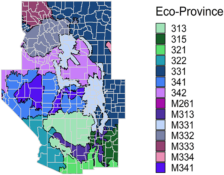
Figure 1. A map of counties in the Interior West, colored by eco-provinces.

FIA data retrievals and processing of auxiliary data were done through the R package FIESTA (Frescino et al., 2020). In summary, we have the following data for each county d and each response variable:

• {y_i, x_i, z_i, f_i}_i∈sd where the data for plot i includes y_i, the value of the forest inventory/response variable, x_i, the TCC value, z_i, the eco-province, and f_i, the post-strata classification.

• {x_i}_i∈Ud, the TCC values for each unit in county d.

• ${\left\{w_{pl}\right\}}_{l=1}^{14}$, a set of weights where each weight represents the proportion of county d in a given eco-province.

• ${\left\{w_{sl}\right\}}_{l=1}^2$, a set of weights where each weight represents the proportion county d in a given post-stratum.

2.2. Estimators

In this section, we formally introduce the GREG and its extension, the GREGORY. We also present the post-stratified estimator (PS), which is featured in our analyses since it is the standard estimator used in FIA's production processes. Additionally, we address variance estimation and provide two variance estimators. All data analysis was done in the statistical software package R (R Core Team, 2020) and the estimators were computed using the gregRy package (Olson and Wojcik, 2021).

2.2.1. The Generalized Regression Estimator

The GREG for μ_yd is given by

$\begin{array}{ll}{\widehat{\mu }}_{y_d,GREG}=\frac{1}{n_d}{\displaystyle \sum _{i\in s_d}}\left(y_i-\widehat{m}(x_i)\right)+\frac{1}{N_d}{\displaystyle \sum _{i\in U_d}}\widehat{m}(x_i)& (1)\end{array}$

where for county d, $\widehat{m}(x_i)$ is the model prediction for unit i based on the predictor vector $x_i^T=(1,x_i)$. When we assume a linear regression assisting model, then $\widehat{m}(x_i)=x_i^T\widehat{\beta }$ with estimated least squares regression coefficients, ${\widehat{\beta }}^T=({\widehat{\beta }}_0,{\widehat{\beta }}_1)$, given by

$\widehat{\beta }={\text{argmin}}_{\beta }{\displaystyle \sum _{i\in s_d}{\left(y_i-x_i^T\beta \right)}^2}.$

In Equation (1), the first term, the average residuals component, ensures that the estimator is asymptotically unbiased since it compensates for any under- or overestimation caused by the second term, which provides the average predicted value. This second term is commonly called the synthetic estimator (Rao and Molina, 2015). Notice that the GREG is only constructed using data within the domain of interest, U_d, and in particular that the estimated regression coefficients are computed using only s_d. When n_d is small, the variance of the estimated coefficients may be large, which in turn increases the variance of ${\widehat{\mu }}_{y_d,GREG}$. Another potential concern is bias. If n_d is small, the property of asymptotic unbiasedness of the estimator may no longer hold. The GREGORY attempts to overcome these issues by fitting the model using not just s_d but also using ecologically similar sample data.

2.2.2. The Generalized Regression Estimator Over Resolutions of Y

For the GREGORY, the estimator form is still given in Equation (1) but now the models are estimated over a larger region. To differentiate between the different data sources, we call the sample data used in estimation, s_d, the estimation sample while that used in modeling is called the modeling sample. For our data application, the resolution of the modeling samples are eco-provinces and so the estimated model prediction for unit i is given by a weighted sum of regression models,

$\widehat{m}(x_i)=x_i^T\left({\displaystyle \sum _{l=1}^P{w}_{pl}}\widehat{{\beta }_l}\right),$

where the estimated regression coefficient vector for province l come from

$\widehat{{\beta }_l}={\text{argmin}}_{\beta }{\displaystyle \sum _{i\in s}{\left(y_i-x_i^T\beta \right)}^2}I(z_i=l).$

Recall that z_i specifies the eco-province of unit i. By separating the estimation and modeling samples, we are able to estimate the models using larger sample sizes and eco-province samples that are likely more ecologically homogeneous than those created by the arbitrary political boundaries of counties. If an estimation sample is nested in a modeling sample, then $\widehat{m}(x_i)$ reduces to a single regression equation. While we focus on weighting simple linear regression models here, more nuanced correlation structures that allow for spatial and/or temporal autocorrelation could be incorporated through a mixed-model approach.

2.2.3. Post-stratification

The PS is a special case of a GREG where a single categorical predictor is used in the regression assisting model. In this case, the estimator of μ_yd simplifies to a weighted sum of post-strata means,

$\begin{array}{cc}\hfill {\widehat{\mu }}_{y_d,PS}=& {\displaystyle \sum _{j=1}^2}{w}_{sj}{ȳ}_j,\hfill \end{array}$

where ${ȳ}_j=n_{dj}^{-1}\sum _{i\in s_d}{y}_{i}I(f_i=j)$, the sample mean of y for post-stratum j and n_dj is the number of sampled plots in post-stratum j for county d. Recall that w_sj is the proportion of county d in post-stratum j.

2.2.4. Variance Estimation

Särndal et al. (1992) provide the standard variance estimator of the GREG,

$\begin{array}{ll}\hat{V}({\widehat{\mu }}_{y_d})=\left(1-\frac{n_d}{N_d}\right)\frac{1}{n_d}\frac{1}{n_d-1}{\displaystyle \sum _{i\in s_d}}{\left(y_i-\widehat{m}(x_i)\right)}^2,& (2)\end{array}$

which can also be used to estimate the variance of the GREGORY. However, the form of the variance estimator relies on large sample approximations and does not account for model estimation variation. Note that the model coefficients of the GREG are chosen to minimize the sum of the squared errors over s_d. Therefore, equation (2) will always report a smaller value for GREG than GREGORY, by construction. However, the true variance of the GREGORY may in fact be smaller than the variance of the GREG since its modeling sample is typically larger and therefore its model estimation variance is likely smaller. To compare the efficiency of the estimators, we want a variance estimator that accounts for both the variability in the residuals and the variability induced by fitting the model. Therefore, in our data application we estimate the variance of the estimators not using Equation (2) but using the following bootstrap variance estimator

${\hat{V}}_B({\widehat{\mu }}_{y_d})=\left(\frac{n_d}{n_d-1}\right)\left(\frac{N_d-n_d}{N_d-1}\right)\frac{1}{B-1}{\displaystyle \sum _{b=1}^B}{({\widehat{\mu }}_{y_d}^{(b)}-{\bar{\widehat{\mu }}}_{y_d})}^2$

where ${\widehat{\mu }}_{y_d}^{(b)}$ is the bth bootstrap estimate and ${\bar{\widehat{\mu }}}_{y_d}=B^{-1}\sum _{b=1}^B{\widehat{\mu }}_{y_d}^{(b)}$ is the average of the bootstrapped estimates. See Mashreghi et al. (2016) for more details on using bootstrap methods in survey estimation.

Returning to the standard variance estimator, it is important to understand the degree of its negative bias since it is commonly used in practice. For simple models and moderately large sample sizes where model estimation variability accounts for little of the overall variance, the standard variance estimator tends to be slightly negatively biased. For more complex models, Kangas et al. (2016) found that this variance estimator can significantly underestimate the true variance. In the simulation study, we explore and compare the bias of the standard variance estimator for both the GREG and the GREGORY across a range of sampling fractions. This allows us to study how the size of the modeling sample impacts the biasedness of the variance estimator.

3. Results

In the data application and simulation study, we compare how county level models vs. eco-province level models impact the model-assisted estimator, especially as we vary the sampling intensity within the counties. While we considered four response variables, we present the results for estimating the average trees per acre in this section. We found similar patterns for the other three response variables.

3.1. Case Study

Our data application investigates the impact of leveraging more data when estimating the model for a modified GREG. We focus on producing county level estimates of the mean trees per acre for the IW and compare the performance of the PS and GREG, which uses only data within the domain, to the GREGORY, which uses additional data from outside the domain. We also consider the modified GREG which uses the entire IW sample for model fitting.

The first step is to determine the resolution of the model samples for the GREGORY, which could range from using just the sampled plots in the county of interest to the entire set of sampled plots in the IW to something in between. Using just the sampled plots, as the GREG does, runs the risk of high variance in its estimates, especially for small sample sizes. On the other hand, using the entire sample, as the modified GREG does, could also be ill-advised if it means lumping together heterogeneous landscapes where the relationship between TCC and trees per acre may vary. And, though GREG is asymptotically unbiased, concerns of bias arise from the small sample sizes of areas being estimated. To reduce the bias of the eventual estimate in finite samples, it would be ideal to estimate GREGORY's model using plot data from areas that have a similar relationship between TCC and trees per acre as that found in the county of interest. Keeping this in mind, we constructed modeling samples based on ecology, in particular, the eco-provinces given by Cleland et al. (2007). When considering at what level to estimate our models, we were motivated to utilize the eco-province level after considering the different levels of ecologies used by FIA. The principal map unit design criterion for eco-provinces is the dominant potential natural vegetation, compared to more granular levels such as eco-sections, which are delineated by the physical and biological components of an ecology such as climate, physiography, lithology, soils, and potential natural communities (McNab et al., 2007).

Figures 2–4 allow for a spatial look at how the relative efficiencies of the estimators, given by the ratio of the estimated bootstrapped variances, compare to one another when estimating the average count of trees per acre for each county. A county is gray if all county plots had a response value of 0 and therefore a variance estimate of 0 for PS or GREG. GREGORY and modified GREG circumvent this issue by using data from outside of these problematic counties. As seen in Figure 2, the GREGORY has a lower variance estimate than the PS for most counties (71%). This trend was similar when comparing GREG to PS. However, we see from Figure 3 that GREG and GREGORY are roughly matched in the number of counties in which one outperforms the other (with GREGORY outperforming 53% of the time). This implies that constructing the model over a larger resolution did not, generally, reduce the variance of the estimates.

FIGURE 2

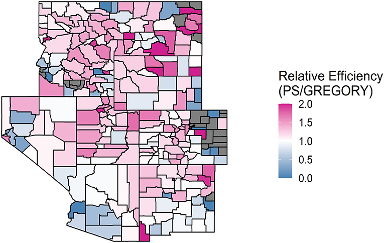
Figure 2. A map of the relative efficiencies of the PS to the GREGORY when estimating the average trees per acre for each county in the Interior West. Values above 1 indicate that the GREGORY is more efficient. Values greater than 2 were truncated to 2 to increase the readability of the map. A county is gray if the RE is 0, due to all plots containing values of 0 trees per acre.

FIGURE 3

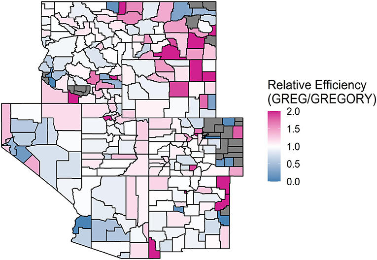
Figure 3. A map of the relative efficiencies of the GREG to the GREGORY when estimating the average trees per acre for each county in the Interior West. Values above 1 indicate that the GREGORY is more efficient. Values greater than 2 were truncated to 2 to increase the readability of the map. A county is gray if the RE is 0, due to all plots containing values of 0 trees per acre.

FIGURE 4

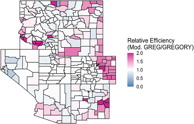
Figure 4. A map of the relative efficiencies of the modified GREG to the GREGORY when estimating the average trees per acre for each county in the Interior West. Values above 1 indicate that the GREGORY is more efficient. Values greater than 2 were truncated to 2 to increase the readability of the map.

We can expand the modeling sample even further, as the modified GREG does, and compare that to the GREGORY, as seen in Figure 4. While GREGORY only outperformed the modified GREG 54% of the time, the precision gains were rather large for some counties and the precision losses were not as extreme. On average, the estimated variance of the modified GREG is 1.14 times the estimated variance of the GREGORY, suggesting that building the model over ecologically homogeneous samples can improve the efficiency of the estimator.

It should be noted that we did see a higher degree of variability in the estimated slopes (${\widehat{\beta }}_1$) for the county level models than the eco-province level models (see Figure 5). We conjecture that this extra variability did not translate into higher variance estimates because the predictive accuracy of the estimated model is a much more dominant component of the variance. This actually provides justification for the standard variance estimator, given in Equation (2), only being a function of the prediction errors and not accounting for model estimation variability. In the next section, we conduct a simulation study to more concretely compare the variability and bias of the estimators as the sample size shrinks.

FIGURE 5

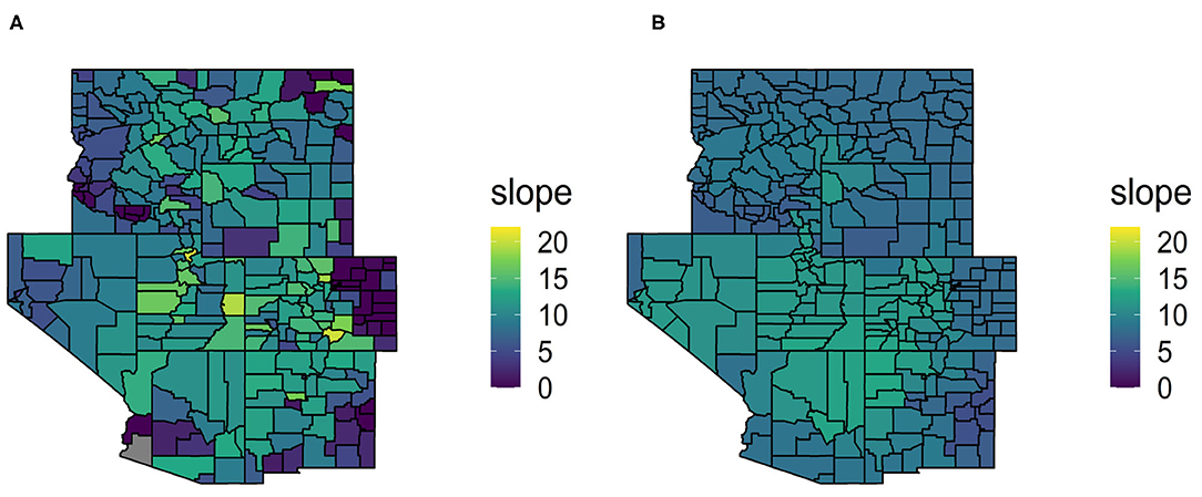
Figure 5. Map (A) contains the estimated slopes of the linear regression model of trees per acre based on TCC for each county in the GREG when the models are fit at the county level. Map (B) contains the estimated slopes for each county in the GREGORY when the models are fit at the province level.

3.2. Simulation Study

The application in the previous section compares estimated variances and so observed differences may be due to random variability and are not necessarily indicating that one estimator is truly more precise than another in a given county. To better understand how the modeling sample size impacts the estimator's bias and precision, we conducted a simulation study. We treated part of the IW as the true, finite population and drew 1000 Monte Carlo samples from the population. By using the plot data as the population, we know the true mean trees per acre for each county and therefore can obtain both the percent relative bias and the empirical mean squared error for the estimators, along with the percent relative bias of the standard variance estimator, by averaging across the samples. Due to the computational intensity of the bootstrap variance estimator, we only measure the bias of the standard variance estimator, given by Equation (2), in this study.

To ensure we had enough data and sampling variability, we selected for the population the 5 IW Mountain eco-provinces which each had at least 3,000 plots. Within these 5 eco-provinces, we selected the counties which had at least 200 plots and where a majority of the county plots were in the selected eco-provinces. It should be noted that we did not include plots from outside these 5 eco-provinces, even if they were in one of the selected counties. Table 1 contains information on the 37 counties that comprised the finite population. For each replicate sample, we randomly sampled p% of each county. To explore the effect of sampling intensity, we varied p from 2 to 10 in 0.5 increments.

TABLE 1

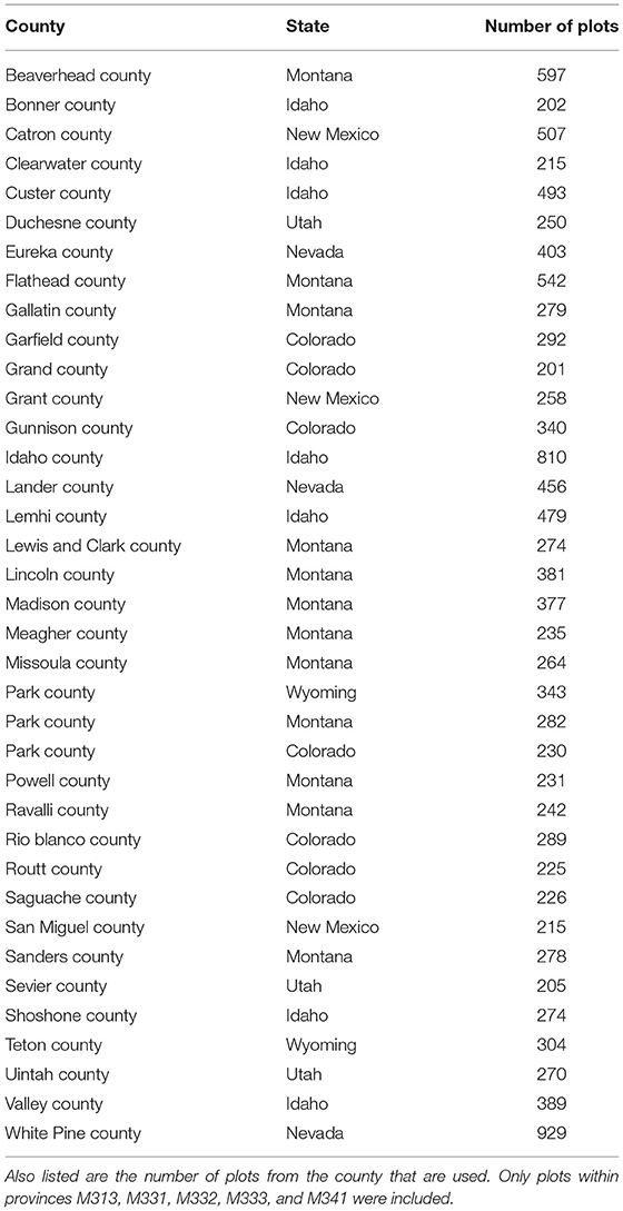
Table 1. Table of the counties included as domains in the simulation.

While the GREG and GREGORY are asymptotically unbiased, the estimators are applied in practice to samples with finite sample sizes. Therefore, it is important to study the degree of bias in the estimators and their variance estimators, especially as a function of sample size. Figures 6, 7 capture the percent relative bias of the estimators across the sampling fractions and sample sizes. Both estimators exhibit little bias for the moderate to large sampling intensities but for the smallest intensities the GREG's percentage relative bias across the 37 counties is rather variable, more so than the GREGORY's.

FIGURE 6

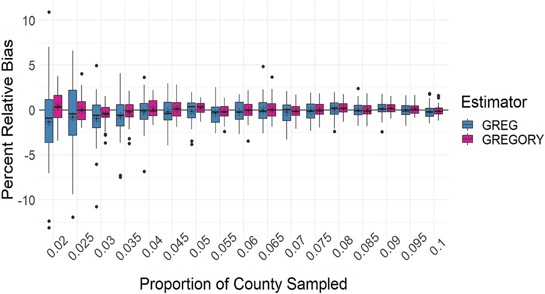
Figure 6. Boxplots of the percent relative bias of the county estimates of average trees per acre across the sampling intensities. The average percent relative bias is denoted by the stars.

FIGURE 7

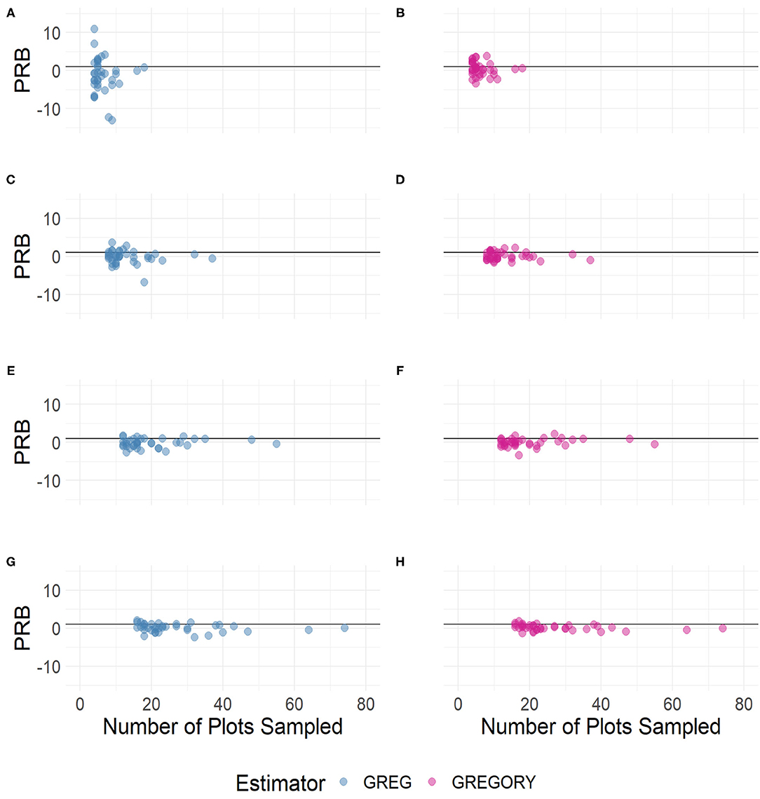
Figure 7. The percent relative bias of the county estimates of average trees per acre by sample size across the following sampling intensities: (A,B) 2%, (C,D) 4%, (E,F) 6%, and (G,H) 8%.

Figures 8, 9 compare the mean square error of the GREGORY and the GREG across the sampling fractions and sample sizes. For the lower sampling fractions, the GREG MSE is more variable and larger, on average, than the MSE of the GREGORY. From Figure 8, we see that the GREGORY is typically more efficient than the GREG for smaller sample sizes and then the estimators perform similarly once a county has at least 30–40 sampled plots. This result demonstrates an advantage to using GREGORY in settings where data are sparse.

FIGURE 8

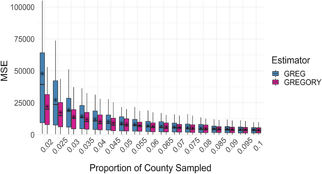
Figure 8. Boxplots of the mean squared error of the county estimates of average trees per acre across the sampling intensities. The average mean squared error is denoted by the stars.

FIGURE 9

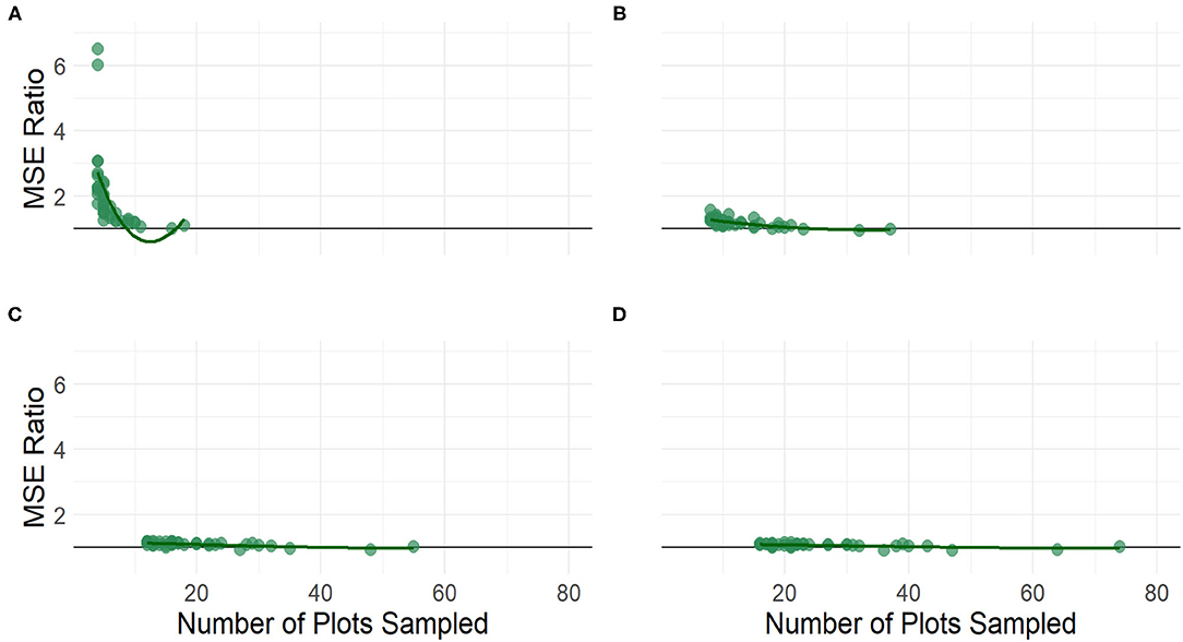
Figure 9. The MSE ratio of the GREG to the GREGORY when estimating the average trees per acre at the county level by sample size across the following sampling intensities: (A) 2%, (B) 4%, (C) 6%, and (D) 8%. A loess smoother is included.

The distributions of the percent relative bias of the standard variance estimator, given in Equation (2), are displayed in Figures 10, 11. The variance estimators for both the GREG and GREGORY are negatively biased for the smaller sampling intensities but the GREGORY is less so. And by a sampling fraction of around 6.5%, or a sample size of at least 20, the variance estimator of the GREGORY exhibits little bias, while the GREG variance maintains some amount of negative bias, even for the largest sample sizes.

FIGURE 10

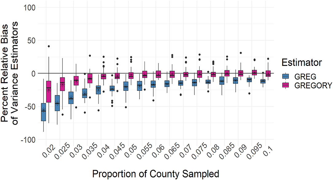
Figure 10. Boxplots of the percent relative bias of the standard variance estimator when estimating the average trees per acre across the sampling intensities. The average percent relative bias is denoted by the stars.

FIGURE 11

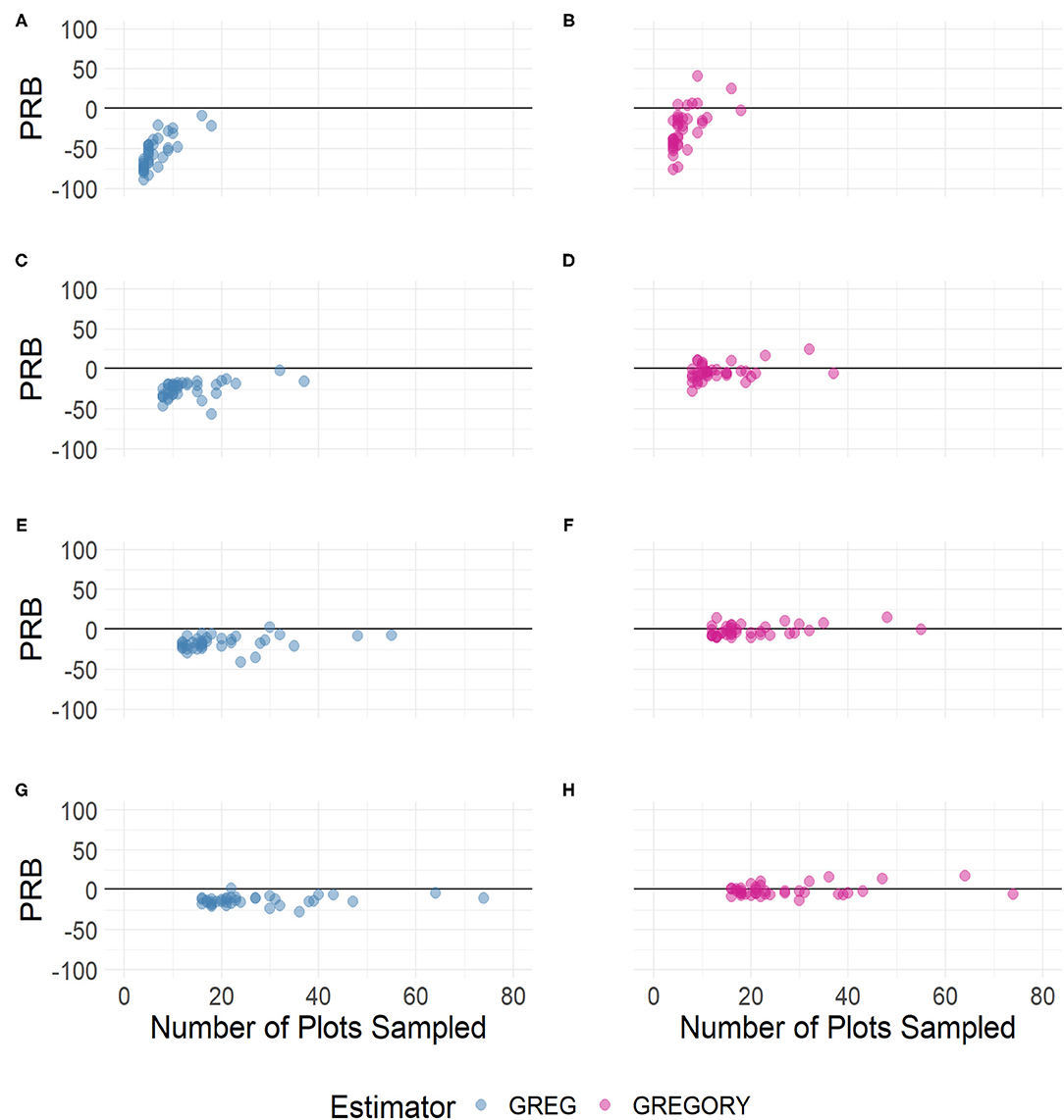
Figure 11. The percent relative bias of the county standard variance estimator when estimating the average trees per acre by sample size across the following sampling intensities: (A,B) 2%, (C,D) 4%, (E,F) 6%, and (G,H) 8%.

4. Conclusion

This paper considers how the variability of a direct estimator is impacted when the assisting model is built using data from a larger region, some of which falls outside the domain of interest. We found that efficiency gains are achieved from these larger modeling samples when the sample size within the domain of interest is small.

A key interest for a practitioner is under what conditions to use GREGORY instead of GREG. We believe this primarily comes down to four questions. First, does survey data exist beyond the domains of interest that samples similar domains? Here, we used eco-province boundaries to identify similar areas that resulted in less variable estimates and avoided the problem of introducing bias caused by modeling from completely different populations. If the entire sample region is ecologically similar, then the modified GREG, which utilizes all the sample data to fit the model, should be considered. Second, does borrowing over this larger region result in diverse models? In our case, adjacent eco-provinces in the Interior Western US are often dramatically different due to topography, but borrowing over a larger area that is quite homogeneous could have little impact on the performance of estimators. Third, are there domains of interest with small sample sizes? In our application in the Interior West, enough data were available and the GREG was adequate for the situation. However, our simulation results show that GREGORY generally produced less biased estimates and better relative precision than GREG as sample size decreased. And fourth, how will the uncertainty of the estimates be calculated? We found that the standard variance estimator exhibited less negative bias for the GREGORY and eventually showed little bias for moderate sample sizes. On the other hand, the standard variance estimator of the GREG continued to exhibit negative bias across all sampling intensities. Lastly, we'd note that for very small sample sizes, a practitioner should consider model-based methods which more directly leverage information from outside the domain as these methods are likely to be more efficient.

Whether fitting a GREG or a GREGORY, there are additional considerations for a practitioner about what assisting model to employ and what auxiliary data to incorporate. These choices should be guided by extensive exploratory data analyses and visualizations. For the GREGORY, we fit separate linear models for each eco-province and then for each county, weighted the eco-province estimated model coefficients by the proportion of the eco-province in the county. There are many other potential approaches, such as building a single model with eco-province indicator functions or taking a mixed-model approach with eco-province random effects. Time spent up front thinking about the model, how the estimated model coefficients may vary across subsets, the inclusion of relevant ancillary data, spatial variations in the data, and domain sample sizes may be profitable by increasing the precision of particular small area estimates, in addition to motivating the choice between GREG and GREGORY.

For understanding operational implications for FIA, GREGORY should be evaluated as an alternative to post-stratification for more response variables, over different geographic regions, and using alternative auxiliary information. Further, much work is underway to expand forest inventory capacity to address new user needs through small area estimation. Through GREGORY, new investigations can determine just how far FIA can push direct, model-assisted estimators suitable for generic inference to meet small domain needs before turning to model-based methods.

Data Availability Statement

The data analyzed in this study is subject to the following licenses/restrictions: the data include confidential plot data, which can not be shared publicly. FIA data can be accessed through the FIA DataMart (https://apps.fs.usda.gov/fia/datamart/datamart.html). Requests for data used here or other requests including confidential data should be directed to FIA's Spatial Data Services (https://www.fia.fs.fed.us/tools-data/spatial/index.php). Requests to access these datasets should be directed to https://apps.fs.usda.gov/fia/datamart/datamart.html, https://www.fia.fs.fed.us/tools-data/spatial/index.php.

Author Contributions

OW, SO, P-HN, KM, GM, and TF: conceptualization. OW, SO, P-HN, KM, and GM: methodology and review and editing. OW, SO, and P-HN: analysis and data visualization. TF: data curation. OW, SO, P-HN, and KM: writing. OW and SO: software. KM: supervision. GM: funding acquisition. All authors have read and agreed to the published version of the manuscript.

Funding

This work was supported by the USDA Forest Service, Forest Inventory and Analysis Program (via agreement 19-JV-11221638-112) and by Reed College.

Conflict of Interest

The authors declare that the research was conducted in the absence of any commercial or financial relationships that could be construed as a potential conflict of interest.

Publisher's Note

All claims expressed in this article are solely those of the authors and do not necessarily represent those of their affiliated organizations, or those of the publisher, the editors and the reviewers. Any product that may be evaluated in this article, or claim that may be made by its manufacturer, is not guaranteed or endorsed by the publisher.

Acknowledgments

The authors would like to thank the USDA Forest Service, Forest Inventory and Analysis Program for the data. The authors would also like to sincerely thank the handling editor and two reviewers for their thorough and constructive comments and suggestions. The reviews really helped us create a clearer and more complete final version of the article.

References

Baffetta, F., Fattorini, L., Franceschi, S., and Corona, P. (2009). Design-based approach to k-nearest neighbours technique for coupling field and remotely sensed data in forest surveys. Remote Sens. Environ. 113, 463–475. doi: 10.1016/j.rse.2008.06.014

CrossRef Full Text | Google Scholar

Blackard, J., Finco, M., Helmer, E., Holden, G., Hoppus, M., Jacobs, D., et al. (2008). Mapping US forest biomass using nationwide forest inventory data and moderate resolution information. Remote Sens. Environ. 112, 1658–1677. doi: 10.1016/j.rse.2007.08.021

CrossRef Full Text | Google Scholar

Breidt, F. J., and Opsomer, J. D. (2017). Model-assisted survey estimation with modern prediction techniques. Stat. Sci. 32, 190–205. doi: 10.1214/16-STS589

PubMed Abstract | CrossRef Full Text | Google Scholar

Cleland, D. T., Freeouf, J. A., Keys, J. E., Nowacki, G. J., Carpenter, C. A., and McNab, W. H. (2007). Ecological Subregions: Sections and Subsections for the Conterminous United States. Available online at: https://www.fs.fed.us/research/publications/misc/73326-wo-gtr-76d-cleland2007.pdf

Google Scholar

Frescino, T. S., Moisen, G. G., Patterson, P. L., Toney, C., and Freeman, E. A. (2020). “Demonstrating a progressive FIA through fiesta: a bridge between science and production,” in Brandeis, T. J., comp. Celebrating progress, possibilities, and partnerships: Proceedings of the 2019 Forest Inventory and Analysis (FIA) Science Stakeholder Meeting; November 19-21, 2019 (Knoxville, TN. e-Gen. Tech. Rep. SRS-256; Asheville, NC: US Department of Agriculture Forest Service, Southern Research Station), 199–200.

Google Scholar

Gregoire, T. G., Såthl, G., Nsset, E., Gobakken, T., Nelson, R., and Holm, S. (2011). Model-assisted estimation of biomass in a LiDAR sample survey in hedmark county, norway. Can. J. Forest Res. 41, 83–95. doi: 10.1139/X10-195

CrossRef Full Text | Google Scholar

Kangas, A., Myllymki, M., Gobakken, T., and Nsset, E. (2016). Model-assisted forest inventory with parametric, semiparametric, and nonparametric models. Can. J. Forest Res. 46, 855–868. doi: 10.1139/cjfr-2015-0504

CrossRef Full Text | Google Scholar

Mashreghi, Z., Haziza, D., and Lger, C. (2016). A survey of bootstrap methods in finite population sampling. Stat. Surveys 10, 1–52. doi: 10.1214/16-SS113

PubMed Abstract | CrossRef Full Text | Google Scholar

McConville, K. S., Moisen, G. G., and Frescino, T. S. (2020). A Tutorial on model-assisted estimation with application to forest inventory. Forests 11:244. doi: 10.3390/f11020244

CrossRef Full Text | Google Scholar

McNab, W. H., Cleland, D. T., Freeouf, J. A., Keys, J. E., Nowacki, G. J., and Carpenter, C. A. (2007). Description of ecological subregions: Sections of the conterminous united states. General Technical Report (GTR), U.S. Department of Agriculture, Forest Service.

Google Scholar

McRoberts, R. E. (2010). Probability-and model-based approaches to inference for proportion forest using satellite imagery as ancillary data. Remote Sens. Environ. 114, 1017–1025. doi: 10.1016/j.rse.2009.12.013

CrossRef Full Text | Google Scholar

Moser, P., Vibrans, A. C., McRoberts, R. E., Nsset, E., Gobakken, T., Chirici, G. O., et al. (2017). Methods for variable selection in LiDAR-assisted forest inventories. Forestry 90, 112–124. doi: 10.1093/forestry/cpw041

CrossRef Full Text | Google Scholar

Olson, S., and Wojcik, O. (2021). gregRy: GREGORY Estimation. Available online at: https://cran.r-project.org/web/packages/gregRy/index.html

R Core Team (2020). R: A language and environment for statistical computing. Vienna : R Foundation for Statistical Computing. Available online at: https://www.R-project.org/

Google Scholar

Rao, J. N., and Molina, I. (2015). Small Area Estimation. Hoboken, NJ: John Wiley & Sons.

Google Scholar

Reams, G. A., Smith, W. D., Hansen, M. H., Bechtold, W. A., Roesch, F. A., and Moisen, G. G. (2005). “The forest inventory and analysis sampling frame,” in The Enhanced Forest Inventory and Analysis Program—National Sampling Design and Estimation Procedures (Asheville, NC: US Dep't of Agriculture, Forest Service, Southern Research Station), 11–26.

Google Scholar

Särndal, C. E., Swensson, B., and Wretman, J. (1992). Model Assisted Survey Sampling. New York, NY: Springer-Verlag.

Google Scholar

Ståhl, G., Saarela, S., Schnell, S., Holm, S., Breidenbach, J., Healey, S. P., et al. (2016). Use of models in large-area forest surveys: comparing model-assisted, model-based and hybrid estimation. Forest Ecosyst. 3:5. doi: 10.1186/s40663-016-0064-9

CrossRef Full Text | Google Scholar

U.S. Department of Agriculture (2014). Farm Bill. Available online at: https://www.congress.gov/113/plaws/publ79/PLAW-113publ79.pdf

Woodruff, R. S. (1966). Use of a regression technique to produce area breakdowns of the monthly national estimates of retail trade. J. Am. Stat. Assoc. 61, 496–504.

Google Scholar

Yang, L., Jin, S., Danielson, P., Homer, C., Gass, L., Bender, S. M., et al. (2018). A new generation of the united states national land cover database: requirements, research priorities, design, and implementation strategies. ISPRS J. Photogrammetry Remote Sens. 146, 108–123. doi: 10.1016/j.isprsjprs.2018.09.006

CrossRef Full Text | Google Scholar