Reliably mapping low-intensity forest disturbance using satellite radar data

1. Introduction

Forests are the major component of the terrestrial ecosystem (Pan et al., 2013), covering 31% of Earth's total land area (FAO, 2020). They play a key role in modulating the climate system (Mitchard, 2018; Nunes et al., 2020) and provide an essential source of livelihood and socio-cultural identity to local communities. The tropical biome has the largest proportion of the world's forests and the richest biodiversity, hosting 50–90% of all terrestrial species (Hoang and Kanemoto, 2021). Unfortunately, tropical forest cover has been declining annually over the last 30 years (Hansen et al., 2013; FAO, 2020), contributing to anthropogenic greenhouse gas emissions (Federici et al., 2015), biodiversity losses (Giam, 2017), disturbances in the terrestrial water cycle (D'Almeida et al., 2007), and a potential increase of infectious diseases (Castro et al., 2019; Beuchle et al., 2021). Tropical deforestation is largely driven by the expansion of agriculture and tree plantations to meet the increasing demands of global supply chains, mainly in beef and oilseeds (Henders et al., 2015; Pendrill et al., 2019a,b). Knowledge of the spatiotemporal patterns of forest disturbance can greatly contribute toward the conservation efforts; however, forest-based interventions will ultimately be effective only if framed within a critical political ecology perspective, and when the current economic model—the main driver of global deforestation—is challenged (McAfee, 2012; Nielsen, 2014; Poudel et al., 2015; Bayrak and Marafa, 2016; Asiyanbi et al., 2017).

Satellite remote sensing is the most suitable tool for estimating rates and areas of forest canopy loss at large spatial scales and in remote regions (Achard et al., 2010). In the last decade, thanks to technical advancements in remote sensing technology and the availability of satellite imagery at high spatial and temporal resolutions, yearly maps of forest loss, and alert systems tracking forest disturbances in near real-time (NRT) have become operational at the national and global scale (Shimabukuro et al., 2006; Hansen et al., 2013, 2016; Vargas et al., 2019; Reiche et al., 2021). However, the extension and magnitude of finer disturbances, such as those caused by selective logging, is still largely uncertain (Bullock et al., 2020). Recent analyses of long-term disturbances in the Brazilian Amazon have found that forest degradation affects a larger area of land than deforestation (Matricardi et al., 2020). Qin et al. (2021) have estimated that, for the period 2010–2019, 73% of the overall above ground biomass (AGB) losses in the Brazilian Amazon came from forest degradation, and only 27% from deforestation. A 30 year (1990–2019) pantropical analysis of the JRC dataset on Tropical Moist Forest (TMF) by Vancutsem et al. (2021) has shown that during the past 5 years annual deforestation has declined by 5% while forest degradation has increased by 38%, becoming the main contributing factor to forest cover loss (+2.1 million ha/year compared with the period 2005–2014). While the rate of deforestation is affected by the outcome of national territorial policies, the same is not true for the degradation rates, whose patterns are more closely interrelated with the climatic conditions (Vancutsem et al., 2021). Indeed, the JRC-TMF dataset shows that, in the Brazilian Amazon, the area of forest degradation due to selective logging and forest fires remains stable or even increases over the years of decreasing deforestation (Beuchle et al., 2021). These results stress the importance of enhancing the detection accuracy of small-scale forest disturbances, shifting the focus of national policy to monitoring and curbing this form of environmental degradation, which often precedes outright deforestation (Matricardi et al., 2020). In the tropics, monitoring systems relying on optical satellite imagery, such as the Global Forest Watch (GFW) Humid Tropical Forest Alerts (Hansen et al., 2016) and the Brazilian Real-Time System for Detection of Deforestation (Shimabukuro et al., 2006), are inherently limited by cloud cover, cloud shadows, weather conditions, and rapid vegetation regrowth removing the transient signs of the disturbance events (Asner et al., 2004; Shimizu et al., 2019). For accurate monitoring of selective logging and small clearings, frequent and temporally consistent image acquisitions are needed (Herold et al., 2011). At present, Synthetic Aperture Radar (SAR) systems are the most promising tools for mapping forest disturbances in the tropics (Joshi et al., 2016; Bouvet et al., 2018a; Ballére et al., 2021; Reiche et al., 2021), thanks to the ability of the radar signal to penetrate through clouds and to its sensitivity to forest structural parameters (Mitchard et al., 2011b; Joshi et al., 2015). The European Space Agency (ESA) Sentinel-1 mission provides free-of-charge C-band SAR images at 10 m spatial resolution and at high temporal frequencies (6–12 days, depending on location and data type). Sentinel-1 operates at a frequency of 5.405 GHz, corresponding to a wavelength of ≈5 cm. Longer wavelength L-band SAR signal (≈23 cm) is considered more suitable for forest disturbance monitoring and AGB estimation than the shorter wavelength C-band SAR data (Mitchard et al., 2011b; Yu and Saatchi, 2016) because of the rapid signal saturation in high biomass forests (Le Toan et al., 1992; Imhoff, 1995; Joshi et al., 2017). However, recent work has demonstrated how the high spatial resolution combined with the frequent observations of Sentinel-1 can overcome the limitations of C-band radar, showing great potential for mapping small-scale disturbances in an accurate and timely manner (Bouvet et al., 2018b; Reiche et al., 2018, 2021; Hirschmugl et al., 2020; Ballére et al., 2021). Most approaches measured changes in SAR backscatter intensity over time, applying empirical thresholds to distinguish disturbed areas (Verhegghen et al., 2016; Deutscher et al., 2017; Lohberger et al., 2018). Bouvet et al. (2018a) introduced a novel method making use of the geometric effects of SAR shadowing to detect forest disturbances near forest edges. More recently, the first SAR-based alert system, the Radar for Detecting Deforestation (RADD) Forest Disturbance Alert, was developed for monitoring pantropical forests in NRT (Reiche et al., 2021). The RADD system makes use of a Bayesian approach and Gaussian Mixture Models derived from historical time series metrics to calculate the probability of change in each forest pixel (Reiche et al., 2018).

The methods mentioned above are increasingly refining the accuracy of forest disturbance detections in time and space. However, they do not provide information on changes in forest structure, for example related to biomass values or tree canopy heights. Previous research has related L-band backscatter signal to changes in AGB using a regional empirical regression model and bi-temporal ALOS PALSAR imagery (Ryan et al., 2012). Above ground biomass was estimated at the two time points, and then the difference in AGB was calculated by subtracting the two estimates. This method is polluted by error propagation as uncertainties from each map are summed up (Hirschmugl et al., 2020).

The study presented here employs a change detection method based on the cumulative sums (CuSums) of Sentinel-1 time series, to retrieve information on location, time, and magnitude of small-scale forest disturbance, including selective logging. The method was recently proposed for monitoring forest disturbances (Ruiz-Ramos et al., 2020) and tested on a tropical site with promising results (Ygorra et al., 2021). Here, we validate this novel approach on a unique, ground-measured dataset collected by the Forest Degradation Experiment (FODEX) in Gabon and Peru, using a combination of unoccupied aerial vehicle (UAV) Lidar, Terrestrial Laser Scanning (TLS), and forest inventory data of small-scale disturbances caused by selective logging. In this paper, we adopt the term “forest disturbance” to describe a decrease in forest cover, which may result in the full conversion of forested land into another land type (deforestation) or in an altered ecosystem that still retains the definition of forest (Houghton et al., 2012). This includes natural or anthropogenic causes, such as forest fires, selective logging, forest fragmentation, and edge effects. We prefer to use the term forest disturbance over forest degradation, as the former does not contain any attempt at classifying the fate and the nature of the change event, on which we may not have sufficient information (Beuchle et al., 2021; Reiche et al., 2021). As for “low-intensity disturbance,” we refer to an event that results in the removal of less than 50% of forest biomass per hectare (Houghton et al., 2012). In conclusion, the novelties of the present work are: (1) The validation of a SAR-based change detection algorithm on in-situ measurements of tropical forest loss; (2) the design of an empirically-derived, single change metric for retrieving information on location, time, and magnitude of the disturbance; (3) the possibility of scaling the algorithm on larger areas, which will be addressed in the Discussion section.

2. Materials and methods

2.1. Study areas

To ensure the reproducibility of the change detection algorithm, we located our study areas in two distinct tropical forest ecosystems, located in the rainforests of the Amazon basin (Peru) and Central Africa (Gabon) (Figure 1). While having distinct forest types and ecology, we set up experimental disturbance plots and collected as far as possible identical datasets before and after logging, to act as an ideal calibration and validation site for such algorithms.

FIGURE 1

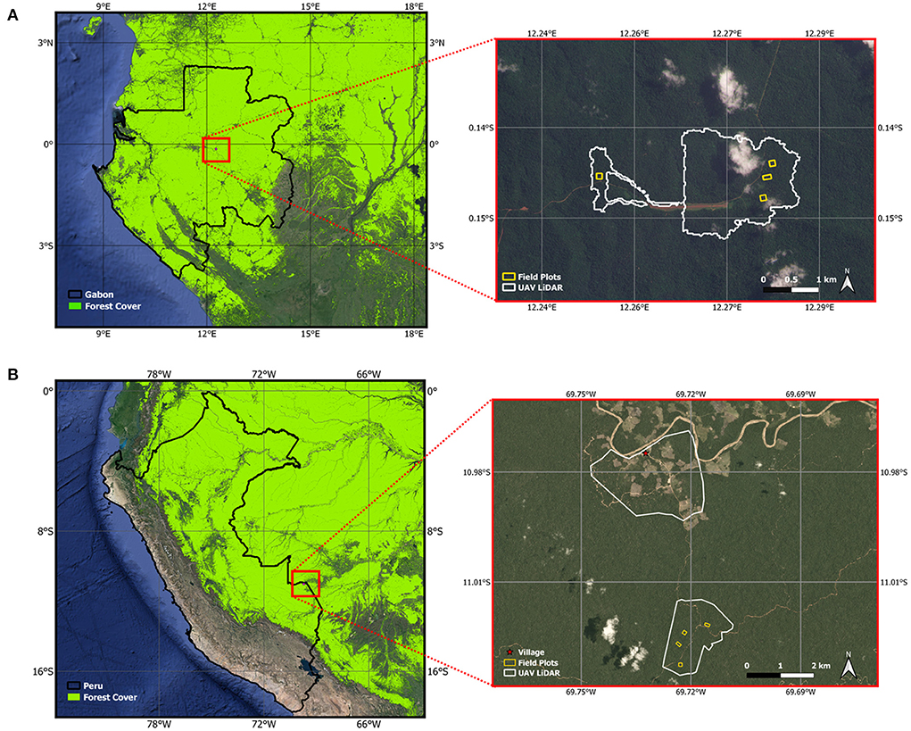
Figure 1. Location of the two study areas in (A) Gabon and (B) Peru. The left panels show the position of the field sites within the country boundaries. The layer in bright green is the primary humid tropical forest extent for the year 2001 from Turubanova et al. (2018). The right panels show the location of the forest plots (yellow boxes) and the area covered by the UAV LiDAR acquisitions (white). Both RGB images of the field sites date to May 2022 and are 3 m PlanetScope images acquired through Planet's Education and Research Program (Planet Team, 2017).

Gabon is the second most forested country in the world, with forests covering about 88% of its surface area (Poulsen et al., 2017). We established our field plots in the Ogooué-Ivindo province, in proximity of a disused airstrip (0.148°S, 12.264°E, Figure 1A) about 9 km North of the Ivindo village. The area is dominated by mixed lowland tropical forest, and is part of a logging concession managed by the French company Rougier Gabon, who harvests principally Aucoumea klaineana (Okoumé) for commercial timber. The logging concession is certified by the Forest Stewardship Council (FSC-C144419) (Carstairs et al., 2022). The climate in the region is sub-equatorial and is characterized by the alternation of two dry seasons (June–August and December–February) and two rainy seasons (September–November and March–April). The average annual temperatures is 24 °C while the annual rainfall is around 1,500 mm year⁻¹, as measured by the Tropical Rainfall Measuring Mission (TRMM 3B43) for the period going from 2009 to 2019 (Adler et al., 2003).

The second study region is located in the the southeastern Peruvian Amazon, in the Madre de Dios department. Madre de Dios is considered a biodiversity hotspot, with 40% of its territory covered by Natural Protected Areas and home to several Indigenous Communities, some of which live in voluntary isolation (Tarazona and Miyasiro-López, 2020). The presence of gold in the soil and river sediment, which is often illegally mined, makes this area particularly vulnerable to environmental degradation (Markham and Sangermano, 2018; Diringer et al., 2020). Deforestation and forest degradation rates have been exacerbated as a result of the construction of the Interoceanic Highway (2006–2012), opening up the area for further development, agriculture, and extractivist operations (Caballero Espejo et al., 2018). We established the field sites in the territory of the Indigenous Bélgica Yine Community (11.02 °S, 69.72 °W, Figure 1B), about 6 km South of the Bélgica village, in an area of planned logging operations. Since 2010, the Bélgica has contracted a logging company, MADERYJA, to carry out FSC-certified timber harvesting within their forest concession (Burga Cahuana, 2013). The area is characterized by lowland tropical rainforest with a well-drained forest floor (terra firme). The climate is warm and humid, with a dry season from May to October and a rainy season from November to April. According to the TRMM precipitation estimates, annual rainfall for this site is around 1,900 mm year⁻¹ for the decade 2009–2019 (Table 1).

TABLE 1

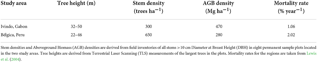
Table 1. Forest structure characteristics of each study site.

2.2. Field data

Four 1-ha Permanent Sample Plots were established in each logging concession and inventoried in two phases, before and after the extraction of selected trees. Standard forest inventory techniques from Phillips et al. (2001) were employed alongside TLS measurements, providing three dimensional models of each tree. We also used a LiDAR sensor mounted on a UAV to collect change data from the wider concession. In Peru the surveyed zone includes the village surroundings, where land conversion due to agricultural expansion is taking place during the dry season, giving areas with greater forest disturbance proportions than the plots (up to 100% AGB loss) (Figure 1B).

2.2.1. Forest inventory

In Gabon, we established four plots in the forested area surrounding a disused airstrip, at an altitude of 500 m and on flat ground, to facilitate the UAV operations (Figure 1A). The plots had an area within 10% of 1 ha and orientations spanning 0–10°North. The position of the plot corners were measured by a differential GPS and corrected using the coordinates of the integrated GNSS receiver of the TLS. Forest inventory campaigns took place in August 2019 and then in February 2020, to account for the removal of 18 trees operated by Rougier Gabon at the end of January 2020. In Peru, we delimited four plots in the forest in proximity of the road that connects Bélgica to Iñapari, at an altitude of 300 m above sea level (Figure 1B). The plots were chosen in consultation with community members and in areas that were rich in valuable timber species, especially for use in community buildings. The plots had an area within 10% of 1 ha and orientations spanning 0–40° North. Forest inventory data was collected in May 2019 and then in October 2020, to measure biomass change resulting from the extraction of 24 trees during the second half of July 2019. In both sites, trees were selectively removed according to FSC logging protocols, in different proportions for each plot, to reproduce a range of degradation events. The Diameter at Breast Height (DBH) of the removed trees ranged between 79–131 cm in Gabon and 50–129 cm in Peru. During the pre-logging campaigns, we adopted the RAINFOR inventory protocols Phillips et al. (2001) to identify, tag, and measure every living stem with DBH > 10 cm. The average DBH recorded was 30 cm in Gabon and 21 cm in Peru, with DBH values ranging between 10–160 and 10–158 cm, respectively. We also collected X and Y coordinates (≈±2 m) and determined tree species information with the assistance of local botanists. Each stem was visually inspected for damage and labeled according to the percentage of its remaining biomass (25, 50, 75, or 90%) as compared to an intact stem of the same size. During the post-logging inventories, as well as remeasuring all the remaining trees, we recorded the direction of tree felling and assessed the collateral damage caused by the logging activities, according to the damage classes described above. Wood density estimates were derived from a global wood density database using tree species information Chave et al. (2009). When possible, we used species-specific wood density values. When multiple wood density values were available for the same taxon, we reported the arithmetic mean. In cases where wood density values were unavailable for a species, we used the average across the genus (29% of the stems); and, where no values were available, we applied the plot average (25% of the stems) (Medjibe et al., 2013).

A pantropical allometric model from Chave et al. (2014) was used to derive total AGB of trees in each plot from DBH (D) and wood density (ρ) values, according to a regional environmental stress factor (E) that averaged −0.096 in Gabon and 0.068 in Peru (Chave, 2014). The equation is in the following form:

$\begin{array}{l}\text{AGB = exp}[-1.803-0.976(E-\text{ln}(\rho ))+2.673\text{ ln}(D)\\ -0.0299\times {\left[\text{ln}\left(D\right)\right]}^2]& (1)\end{array}$

Allometric estimates of AGB at individual tree scale are found to have large uncertainties (Chave et al., 2014) which tend to increase with tree size (Gonzalez de Tanago, 2018; Burt et al., 2021). On the other hand, TLS measurements are found to be in better agreement with the volume data from destructive harvest experiments, with a mean tree-scale relative error of 3% (Burt et al., 2021), thus providing more accurate estimates of AGB values.

2.2.2. Terrestrial laser scanning

Terrestrial Laser Scanning data were collected at the same time as the pre-logging campaigns using a Riegl VZ-400 scanner. The plots were subdivided in 10 × 10 m squares and two scans were obtained at every grid intersection point, following the procedures outlined in (Wilkes et al., 2017). The point clouds of the logged trees, extracted via the treeseg package (Burt et al., 2019), were used to calculate the quantitative structural models of tree volume (QSMs) (Raumonen et al., 2013; Calders et al., 2015). From the QSMs, the AGB of the logged trees was obtained by multiplying wood density by model volume. At the time of the analysis, processed TLS data volumes were only available for the logged trees, hence it was not possible to calculate the total AGB per plot using the TLS measurements. It is important to note that the logged trees in our experiment were, in most cases, the largest trees in the plots, with an average DBH of 102 cm (Gabon) and 79 cm (Peru). To increase accuracy and reduce allometric bias, we adopted TLS-derived biomass estimates for the logged stems. Total AGB change per plot was then calculated by summing the TLS-derived AGB of the logged trees plus the difference in allometric AGB of the remaining trees as measured by the forest inventory surveys (Table 2). Given their smaller sizes, we do not expect significant differences between AGB and TLS-derived estimates for the non-logged trees; on the other hand, if we use allometric equations for the logged trees, then the biomass removed per plot is overestimated by up to 29% in Peru and underestimated by up to 15% in Gabon, as compared to the values derived from the TLS measurements (Table S1, Figure S1).

TABLE 2

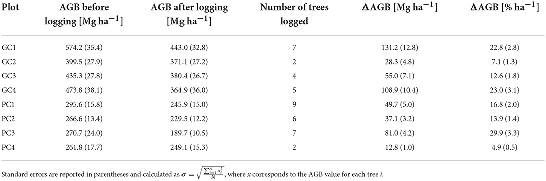
Table 2. Aboveground Biomass (AGB) before and after logging and Aboveground Biomass Change (ΔAGB) figures for eight 1-ha selectively logged plots located in Gabon (G) and Peru (P), obtained by field surveys and Terrestrial Laser Scanning (TLS).

2.2.3. UAV LiDAR

In Gabon, UAV LiDAR data were obtained in January 2020, prior to selective logging in the permanent plots, and then in January 2021, to measure the widespread disturbance resulting from commercial logging operations in proximity of the airstrip, which took place between November and December 2020. In Peru, the first UAV LiDAR campaign took place in May 2019 in conjunction with the pre-logging census. The post-logging LiDAR data were acquired in September 2021, accounting for changes in canopy cover due to selective logging in the study plots and agricultural encroachment in the forest fringes near the village area. For both Gabon censuses, and the first Peru census, a RIEGL miniVUX-1DL LiDAR mounted on a DELAIR DT26X fixed-wing UAV was flown at 140 m above the ground and at a speed of ≈17 ms⁻¹, yielding a point density of 240 pts m⁻². For the post-logging campaign in Peru a LiDAR RIEGL Minivux-2UAV mounted on a rotor craft was used for the UAV data collection, yielding a point density of 200 pts m⁻². Flight trajectories were corrected using post-processing kinematic (PPK) positioning from ground control points and a GNSS base station, resulting in a geometric accuracy of 1.8 cm (McNicol et al., 2021). Canopy height models (CHM) for a total area of 1,239 ha (354 ha in Gabon and 885 in Peru) were generated by taking the difference between the highest and lowest returns in a 25 cm cell and after noise filtering (McNicol et al., 2021). For each site, a ΔCHM raster was obtained by taking the difference between the pre- and post-logging CHMs. Losses in canopy cover were identified as in areas where ΔCHM decreased by 10 m or more (Figure 2).

FIGURE 2

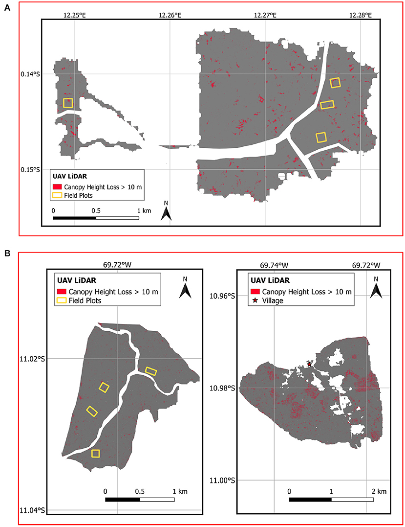
Figure 2. Canopy height change from UAV LiDAR measurements (gray image) showing losses in forest canopy height of more than 10 m (red). (A) Canopy height loss in Gabon from January 2020 to January 2021 indicating patches of disturbance in the study plots and in the surrounding concession; (B) Canopy height loss in Peru from May 2019 to September 2021, showing fine-scale losses in the area of the study plots (left panel) and more intensive, consistent patterns of forest to agriculture conversion in proximity of the village (right panel).

2.3. Sentinel-1 SAR data

The ESA Sentinel-1 mission provides dual-polarization SAR data at high spatial and temporal resolution. The Sentinel-1 constellation comprises two satellites: Sentinel-1A and Sentinel-1B, launched on 3rd April 2014 and 25th April 2016, respectively. Each satellite carries a SAR C-Band instrument onboard operating at a frequency of 5.405 GHz in four different modes. The preferred mode for land use applications is Interferometric Wide-swath (IW) with a ground resolution of 20 × 5 m and a swath width of 250 km. The repeat orbit cycle of each satellite is 12 days over the field sites. The data used in this study were acquired as VV-polarized, ground range detected (GRD) products in IW mode. The provided pixel size is 10 × 10 m. All images were retrieved in descending mode and using the same orbit for each study area (relative orbit number 80 for Gabon and 127 for Peru) to ensure a consistent radar geometry for all the scenes. All available imagery were retrieved from the geospatial cloud computing platform Google Earth Engine (GEE) (Gorelick et al., 2017) using the Python API. Sentinel-1 GRD scenes are provided by GEE already preprocessed and radiometrically calibrated to the backscatter coefficient σ^o in decibels (dB) (Google Earth Engine, 2021).

2.4. Change detection with cumulative sums

The CuSum algorithm is recognized as a powerful statistical method for detecting abrupt and systematic changes in time series data (Page, 1955; Taylor, 2008; Manogaran and Lopez, 2018). While being extensively used for monitoring market trends and industrial processes (Manly and Mackenzie, 2003), it has recently found applications in the environmental sciences for detecting seasonal climate changes (Manogaran and Lopez, 2018) and for monitoring deforestation and forest degradation in temperate (Kellndorfer et al., 2019; Ruiz-Ramos et al., 2020) and tropical forests (Ygorra et al., 2021). Results from Ruiz-Ramos et al. (2020) and Ygorra et al. (2021) have shown the robustness of this method for detecting cover changes in forest canopy, with overall accuracy of 77% and 91%, respectively. However, the data they used to obtain these numbers were produced by visual interpretation of optical satellite imagery, which presents many limitations. Even in 3 m resolution PlanetScope images, degradation effects preceding deforestation cannot be immediately detected, especially in the case of dense and multi-storied canopies. Moreover, and this is particularly relevant in tropical environments, canopy gaps can quickly recover in between two cloud-free images, resulting in a large underestimation of actual forest disturbances (Asner et al., 2004; Shimizu et al., 2019; Ygorra et al., 2021). By contrast in this study we use very high resolution (25 cm) in-situ data from UAV LiDAR to validate the CuSum method in its ability to detect subtle changes in forest canopy resulting from low-intensity logging.

2.4.1. CuSum implementation

Ygorra et al. (2021) found that in tropical forests the co-polarized backscatter (VV) showed best results, as compared to the cross-polarized channel (VH), and this was also confirmed by our preliminary tests. Therefore, time series data stacks were generated using the VV-polarized channel containing the spatial information (range and azimuth) and the temporal dimension for each pixel of the Sentinel-1 image over the study area and for a selected study period. The study period was set as the time of the UAV LiDAR acquisitions (January 2020–January 2021 for Gabon and May 2019–September 2021 for Peru). In order to capture all forest loss in the study period and build the control trend in absence of structural changes, the data cubes included all observations extending from at least 1 year before (reference or pre-change data) to at least 6 months after the UAV measurements (recovering or post-change data). For Gabon the data cube comprised a total of 89 scenes from 6th January 2019 to 21st December 2021; while for Peru a total of 127 scenes from 2nd January 2018 to 18th March 2022 were downloaded.

The cumulative sum of the residuals (CuSum) is defined as the CuSum of the difference between each pixel value and the mean of the timeseries:

$\begin{array}{ll}{R}_{sumj}={\displaystyle \sum _{j=1}^n}{\sigma }_{j,i}^o-\overline{{\sigma }_i^o}& (2)\end{array}$

where ${\sigma }_{j,i}^o$ is the value of each pixel i for each image j, n is the number of images, and $\overline{{\sigma }_i^o}$ is the mean of the time series over each pixel i. Iteratively, CuSum can be written as:

$\begin{array}{ll}{R}_{sumj}=({\sigma }_j^o-\overline{{\sigma }_j^o}+R_{j-1},j=1,2,3,...n)& (3)\end{array}$

where the starting value for the CuSum, R₀, is equal to zero.

Figure 3 compares the resulting CuSum curves for disturbed and undisturbed pixels in two of our field plots, where we have precise information on the location and timing of the change event. For undisturbed pixels, seasonal variations in canopy cover (i.e., phenology), or changes in the moisture content of vegetation result in small fluctuations in the CuSum curve, which, in the absence of structural changes, oscillates around a backscatter value of zero. On the other hand, the CuSum of logged pixels appear like a bell-shaped curve, steadily increasing until a sudden turn in direction. Since $\overline{{\sigma }_i^o}$ is the overall average, a sudden change in direction of the CuSum curve marks a shift or change in the average trend. A downward slope indicates a period of time where the values tend to be below the overall average (Taylor, 2008). Different studies have reported a decrease in the backscatter signal after forest disturbance (Joshi et al., 2015; Reiche et al., 2018; Kellndorfer et al., 2019; Silva et al., 2022), in agreement with what is observed here. As shown by Figure 3, the shift from a positive to a negative trend occurs in coincidence with the time of logging. Hence, the CuSum chart not only gives an indication of change, but it also provides information on when the change has occurred.

FIGURE 3

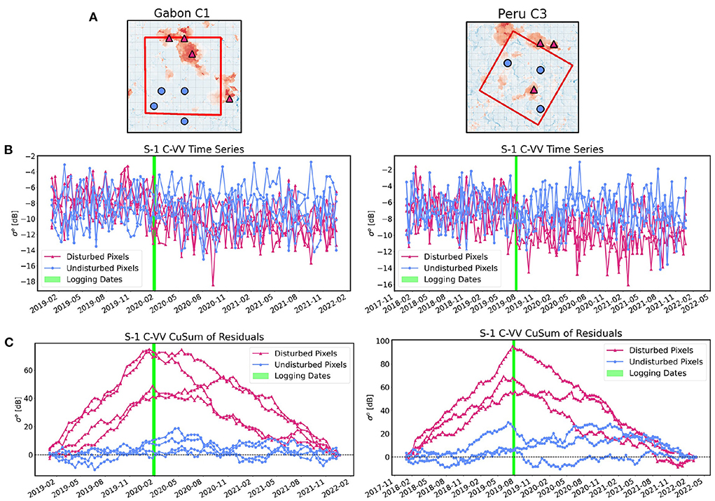
Figure 3. Comparison of disturbed and undisturbed pixels for selectively logged plots in (left) Gabon and (right) Peru. (A) Location of the disturbed pixels (purple triangles) and undisturbed pixels (blue circles) on the Canopy Height Change raster from the UAV LiDAR measurements. Disturbance areas on the LiDAR map are indicated in dark red. (B) Time series of Sentinel-1 (S-1) SAR backscatter values for the disturbed and undisturbed pixels. (C) CuSum curves for the disturbed and undisturbed pixels. Pixels where logging activities took place display a bell-shaped curve peaking around the time of logging (green line).

2.4.2. Threshold estimation and accuracy assessment

Figure 3C implies that it must be possible to distinguish between disturbed and undisturbed pixels by applying a threshold on the peak of the CuSum curve. In-situ data on canopy height loss from the UAV LiDAR measurements can be used as reference data to estimate the optimum value for this threshold, instead of adopting statistical methods (Ruiz-Ramos et al., 2020) or parameterized thresholds (Ygorra et al., 2021). The LiDAR-derived ΔCHM raster (Figure 2) was first resampled by averaging to cells of 10 × 10 m, to allow direct comparison with Sentinel-1 data. We considered a detection as a canopy reduction of 10 m or more and determined the threshold on the value of the CuSum peak, or R_{sum_max}, by matching LiDAR canopy height loss to R_{sum_max} values within the same cell. The overall accuracy of the method is defined as the ratio between the number of real detections and the total number of pixels:

$\begin{array}{ll}OverallAccuracy(OA)=\frac{TP+TN}{TP+TN+FP+FN}& (4)\end{array}$

where TP are the True Positive, i.e., pixels classified as canopy loss by both the LiDAR and the CuSum algorithm; TN are the True Negative, i.e., pixels classified as no change both by the LiDAR and the CuSum algorithm; FP are the False Positive, i.e., pixels classified as change by the CuSum algorithm but not by the LiDAR, and FN are the False Negative, i.e., pixels classified as change by the LiDAR but not by the CuSum algorithm. The threshold was determined as the value of R_{sum_max} that would minimize the False Negative and False Positive detections in the Sentinel-1 observations, in reference to the LiDAR data (Figure 4). Once a threshold on R_{sum_max} was applied, adjacent pixels were grouped into polygons to define the boundaries of each disturbance cluster. The same procedure was also applied to the UAV LiDAR data to extract polygons containing canopy loss values ≥10 m, which were then compared with the disturbance clusters from the CuSum algorithm. The total number of overlaps was calculated by counting the places where the geometries of the two layers intersected. Since the LiDAR data was collected at considerably higher resolution than Sentinel-1 images, small clusters in the LiDAR reference map were grouped into larger clusters by creating a 10 m buffer around each polygon. This step was necessary to avoid double counting LiDAR detections overlapping the same CuSum cluster. We used QGIS software (Polygonize plugin, QGIS version 3.10) to group raster pixels into polygons and to perform all vector operations. The overlap between the polygon datasets was performed using the overlay() method from the geopandas library implemented in Python.

FIGURE 4

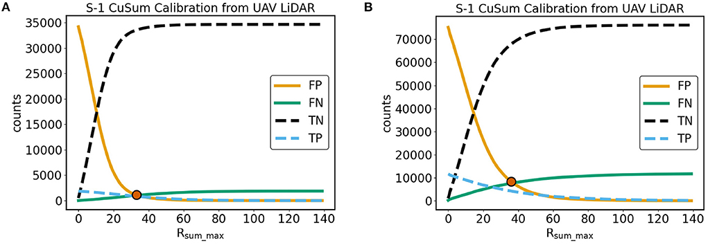
Figure 4. Calculating the value of the CuSum maximum (R_{sum_max}) from Sentinel-1 (S-1) time series that would minimize both False Positive (FP) and False Negative (FN) change detections in (A) Gabon and (B) Peru. The optimum value is indicated by a circle at the point of intersection between the FP and FN curves. Change is defined as a canopy height loss ≥ 10 m as derived from a UAV LiDAR ΔCHM raster resampled to 10 × 10 m pixels. The counts in Peru are double the size than Gabon as here the S-1 time series spans 2 years, consistently with the timeframe of the UAV LiDAR acquisitions. True Positive (TP) and True Negative (TN) curves are also shown in this Figure.

So far we have described CuSum curves peaking at positive values of σ^o, with a sudden shift in the negative direction at the time of logging (Figure 3). Certain pixels in our study areas, however, feature a diametrically opposite trend, with CuSum curves peaking at negative σ^o and then suddenly shifting in the positive direction, meaning an increase in backscatter signal after the change event. Figure 5 shows our study area in Gabon with the location of pixels featuring a negative or positive CuSum, after a threshold was applied on both negative and positive peak values, as found by the processing step outlined in Figure 4. Figure 5 shows how pixels with negative CuSum peaks are spatially symmetric to pixels with positive CuSum peaks. However, by overlaying the UAV LiDAR layer, we have found that only the positive CuSum pixels correspond to areas of canopy height loss (Figure 5C). Hence for this study we have only retained pixels with positive R_{sum_max} values (decreased backscatter), interpreting the latter as canopy gaps, or areas of SAR shadow (Bouvet et al., 2018a), and negative R_{sum_max} values (increased backscatter) as the border between standing forest and the clear-cut (Villard and Borderies, 2007).

FIGURE 5

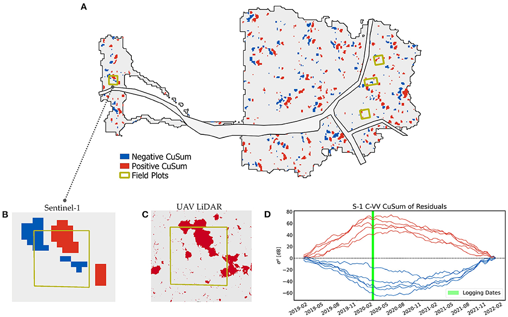
Figure 5. (A) Image of the study area in Gabon, showing in blue the location of pixels with negative CuSum curves and in red the location of pixels with positive CuSum curves, after applying a threshold of R_{sum_max} = 33 for the positive values and R_{sum_max} = -33 for the negative values; (B) Zoom on one of the field plots (Gabon C1), indicating how positive and negative values of R_{sum_max} are arranged symmetrically to each others; (C) The same plot, but with canopy height loss (≥ 10 m) from the UAV LiDAR appearing in red; (D) CuSum curves of five pixels with negative R_{sum_max} (blue lines) and five pixels with positive R_{sum_max} (red lines) selected from the same field plot in panel (B). The time series of the two types of pixels feature diametrically opposite trends, expressing in the time dimension the spatial symmetry that can be seen in (A,B).

Previous studies have found that a CuSum-based change detection method performed better when filtering or smoothing the time-series (Kellndorfer et al., 2019; Ruiz-Ramos et al., 2020; Ygorra et al., 2021). We have tested the detection accuracy of the CuSum algorithm by smoothing the Sentinel-1, VV-polarized time-series with spatiotemporal filters of increasing window sizes, where a size of 1 pixel means that no smoothing was applied. The algorithm was developed using the signal module in Python (Virtanen et al., 2020) and consists of convolving the original time series by a 3D kernel of size w × w × w, where w is the window size (in pixels). Results are shown in Table 3. As accuracy is found to worsen with increasing window size, we did not apply any boxcar filtering to the analysis.

TABLE 3

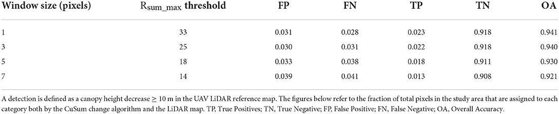
Table 3. Comparison between the CuSum algorithm and the UAV LiDAR reference map in the study area in Gabon, when boxcar filters of increasing window sizes are applied.

2.5. Biomass change estimation

Subsequently to selective logging, a reduction in forest cover amounting to a loss of 5–30% of initial biomass per hectare was field-measured across the eight study plots, corresponding to very low to low-intensity canopy disturbances. For this analysis we also selected four undisturbed plots (ΔAGB = 0%), two for each study site, in areas that did not experience logging activities. To encompass the full spectrum of forest disturbance, we added three plots in Peru that transitioned from forest to agricultural land (ΔAGB = 100%). The 0% and 100% biomass change plots were determined from empirical knowledge of the study area, in addition to visual inspection of the UAV LiDAR reference map and PlanetScope imagery.

Previous work had successfully correlated decreases in L-band radar backscatter to structural changes in vegetation cover (Mitchard et al., 2011a; Ryan et al., 2012; Joshi et al., 2015). However, biomass estimation in tropical forests is inherently limited by the saturation of the radar signal (Mermoz et al., 2015). Shorter wavelength C-band data is generally considered less useful because of even lower penetration depth, as compared to L-band radar (Le Toan et al., 2004; Woodhouse, 2017). On the other hand, Figure 3 shows CuSum curves of logged pixels peaking at different values of σ^o, possibly indicating a variation in the intensity of the change event. For this reason, we tested the sensitivity of the maximum of the CuSum curve, R_{sum_max}, to changes in the AGB values of the study plots, ΔAGB, before and after selective logging. After taking the average value of R_{sum_max} in each plot, we analyzed its relationship with ΔAGB using a linear regression model, taking ΔAGB (in units of % ha⁻¹) as the dependent variable and R_{sum_max} as the independent variable. The linear relationship between the two quantities is in the form y = mx+c. Substituting x with R_{sum_max} from the Sentinel-1 observations (resampled to 1 ha pixels), we obtain ΔAGB values for building a biomass change map of the two regions.

2.5.1. Tree cover loss map from global forest watch

As in-situ biomass change data is not available for the wider regions, we evaluated the performance of the biomass change map in its ability to detect forest loss by comparing it to the GFW Tree Cover Loss (TCL) product from Hansen et al. (2013) for the year 2020. The comparison was performed for the test region in Peru as this area experiences more widespread forest disturbance. Since TCL in the GFW dataset is defined as the complete removal of tree canopy at the Landsat pixel scale (30 m resolution) (Hansen et al., 2013) we compared this product with the ΔAGB map where we only retained values of 100% biomass loss. We resampled the GFW TCL dataset to 1 ha resolution and calculated the amount of 30 m pixels flagged as TCL to retrieve the total disturbance area.

3. Results

3.1. Spatiotemporal patterns of forest disturbance

The CuSum formula from Equation (2) was applied to the time series of VV-polarized Sentinel-1 images acquired over two study areas in Gabon and Peru. The maximum of the CuSum curve, R_{sum_max}, was chosen as the metric for detecting change. Using the UAV LiDAR acquisitions as a reference map, we determined a detection threshold of R_{sum_max} > 33 for Gabon and R_{sum_max} > 36 for Peru (Figure 4), with OA = 94% and OA = 82%, respectively. Figure 6 shows pixels classified as detections after the threshold on R_{sum_max} is applied, as compared to the UAV LiDAR reference map. Change pixels are found to be spatially distributed into clusters, displaying geometrical patterns of forest disturbances. By zooming over two selectively logged plots in each study area, it is possible to observe how the clusters obtained from the CuSum algorithm consistently match patches of canopy loss from the LiDAR measurements. In Gabon, during the study period going from January 2020 to January 2021, the CuSum method detected 240 disturbance clusters covering a total of 14.4 ha (4% of the study area), while field data from the LiDAR measurements estimated 317 clusters of canopy loss ≥ 10 m, for a total of 18.0 ha (5% of the study area). Seventy-eight percent of the disturbance clusters detected with the CuSum method overlapped the location of the LiDAR detections, with both maps having a minimum mapping unit of 0.01 ha (10 × 10 m pixel size). Increasing the minimum size of the CuSum disturbance clusters improved the probability of detection: 91% of the clusters with areas ≥ 0.02 ha matched the LiDAR reference data, while 100% of the clusters with areas ≥ 0.05 ha matched the location of the LiDAR detections. However, increasing the minimum mapping unit reduces the number of detections (Table 4). In Peru, the CuSum time series was filtered for the study period going from May 2019 to September 2021, to match the timeframe of the LiDAR acquisitions. In total, i.e., both in the village area and the field plot site, the CuSum algorithm detected 484 disturbance clusters, with a total area of 57.7 ha (7% of the study area), while the LiDAR reference map estimated 689 disturbance patches, giving a total of 84.8 ha (10% of the study area). 65% of the CuSum detections overlapped the location of the LiDAR disturbances. This figure increased to 90% when considering CuSum clusters ≥ 0.05 ha, and to 99% for CuSum clusters ≥ 0.1 ha (Table 4).

FIGURE 6

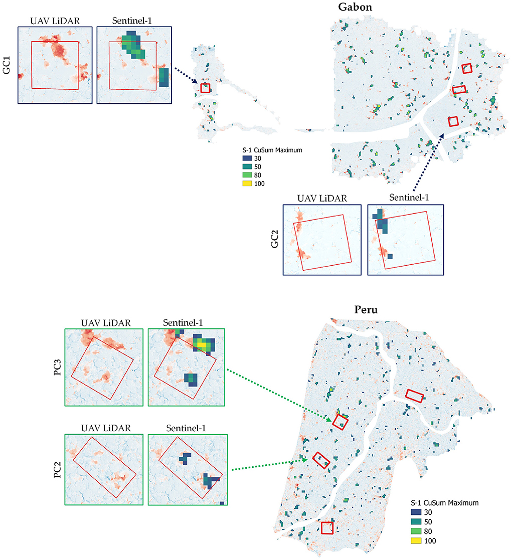
Figure 6. Results of the CuSum change detection algorithm showing the location of the forest disturbance pixels in the study areas in Gabon (top) and Peru (bottom). The inlets are zoomed views of two selectively logged plots for each study area. The left inlets are the UAV LiDAR reference map (25 cm resolution), with areas of canopy height loss appearing in red. The right inlets show clusters of disturbances pixels from the CuSum algorithm applied to Sentinel-1 data overlaid on the LiDAR reference map.

TABLE 4

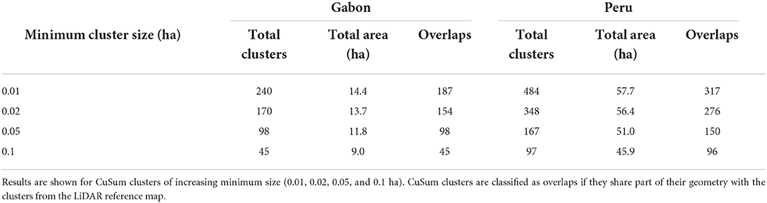
Table 4. Results from the CuSum change detection algorithm showing total number of disturbance clusters, total disturbance area, and total number of overlaps with respect to the LiDAR reference map (Gabon: 317 LiDAR clusters for a total area of 18.0 ha; Peru: 689 LiDAR clusters for a total area of 84.8 ha).

The position of R_{sum_max} in the CuSum chart corresponds to the moment in time immediately before backscatter intensity drops below the historical average. As a result, the time of the disturbance event was derived by selecting the date of the image that follows the date of the inflection point in the time series. Disturbance events were filtered to retain only change pixels within a single year. This was chosen as the year when selective logging occurred in the permanent sample plots, i.e., 2020 for Gabon and 2019 for Peru. Figure 7 shows the timing of the change detections, in units of Day of Year (DOY), in both our study areas. In Gabon, the field plots were selectively logged at the end of January 2020, while commercial logging operations in the surrounding area were carried out between November and December 2020, in coincidence with the second dry season (Figure 7A). In Peru, selected trees were extracted from the study plots during the second part of July 2019, while the rest of the area remained mostly undisturbed (Figure 7B). More significant patches of disturbance are observed near the village during a period going from June to August (Figure 7C). Indeed this time frame corresponds to the peak of the dry season, when forests fringes are cleared for agricultural fields and pasture. These observations have been further confirmed by inspection of PlanetScope imagery and conversations with the Bélgica community.

FIGURE 7

Figure 7. Dates of forest disturbance during the period of interest, determined as the year when the field sites were selectively logged. Dates are reported in Day of Year units (1–366); (A) Dates of forest disturbance in Gabon, for changes during the year 2020; (B) Dates of forest disturbance in Peru, showing changes occurred during the year 2019 in our study areas in proximity of the field sites and (C) near the village.

3.2. Retrieving the magnitude of the disturbance events

Relating the backscatter values of the CuSum maximum to the LiDAR-derived mean canopy height loss per pixel reveals an exponential decay relationship between the two quantities, implying that R_{sum_max} is sensitive to physical changes in forest canopy, from 10 m up to about 50 m in vertical drop (Figure 8). However, the large variations in R_{sum_max} magnitudes at pixel level makes it difficult to derive accurate values of forest canopy loss at this scale.

FIGURE 8

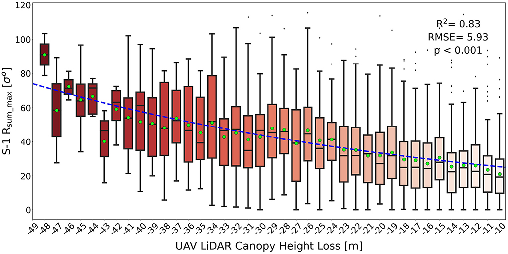
Figure 8. Distribution (boxplots) and means (green circles) of Sentinel-1 CuSum maximum backscatter for each UAV LiDAR measurement of canopy height loss in our study area in Gabon. Data is binned into intervals of canopy height loss of 1 m. The mean values of the distribution follow an exponential decay curve (blue dashed line) in the form y = ae^(−bx), where a = 18.67 and b = 0.03. The coefficient of determination R², the Root Mean Square Error (RMSE) and the p-value are shown on the plot.

On the other hand, a strong correlation between the remotely sensed R_{sum_max} and field-measured ΔAGB was found using a linear regression model with R² = 0.95 and RMSE = 7.90 (p < 0.001) (Figure 9). The CuSum algorithm was applied to Sentinel-1 VV-polarized time series acquired over an area ≈250 times larger than our study site in Gabon (99,938 ha in total) and ≈150 times larger than our study site in Peru (39,559 ha in total). Maps of biomass loss for the year 2020 were produced for both locations from the coefficients of the regression model (Figure 10). In Peru, where forest cut is more widespread, the GFW TCL map estimated a total disturbance area of 348 ha (0.9% of the total area) as compared to 504 ha (1.3% of the total area) from the CuSum-derived biomass map. Sixty-one percent of the detections from the GFW map were found to overlap with the observations of 100% tree canopy loss from the CuSum map. The overlap reached 83, 73, and 90% when AGB loss values from the CuSum map were extended to ΔAGB > 80%, ΔAGB > 60%, and ΔAGB > 50%, respectively (Figure S3).

FIGURE 9

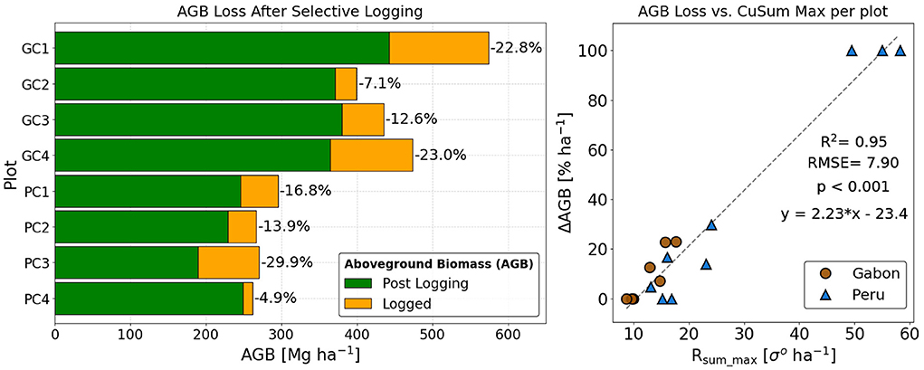
Figure 9. (left) AGB loss in Mg ha⁻¹ in the eight 1-ha selectively logged plots in Gabon (G) and Peru (P); (right) AGB loss (ΔAGB) vs. the maximum of the CuSum curve (R_{sum_max}) for plots in Gabon (brown circles) and Peru (blue triangles). In addition to the eight field-inventoried plots (right), four undisturbed plots (ΔAGB = 0%) and three fully deforested plots (ΔAGB = 100%) were added to the sample data.

FIGURE 10

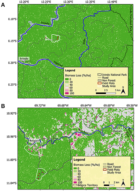
Figure 10. Maps of above ground biomass (AGB) loss (% per hectare) for two areas in (A) Gabon and (B) Peru, with the location of the study sites (white line) and the field plots (red boxes). Non- forest areas have been masked using the primary humid tropical forest extent for the year 2001 from (Turubanova et al., 2018).

3.3. Comparison to RADD alerts

In this section we compare the CuSum change detection algorithm to the RADD disturbance alerts (Reiche et al., 2021), as both are derived from Sentinel-1 data. Radar for Detecting Deforestation Alerts for South America are only available from 2020, hence we chose this year for performing the comparison. As we did with the CuSum layer, RADD alert pixels were grouped into disturbance clusters to allow direct comparison with our results. In our test site in Gabon, the RADD product is able to detect only seven disturbance clusters, as compared to 240 from the CuSum algorithm. All RADD alerts overlap the LiDAR reference map; however, none of the RADD alerts is able to detect logging in our field plots (Figure 11A). In Peru we could not perform the comparison with our selectively logged plots, as timber was extracted during 2019. For this comparison we selected the village site, as this area normally experiences agricultural expansion during each dry season. Here, RADD alerts are able to spot large and spatially continuous patches of deforestation, likely clear cuts for conversion into agriculture and pasture, omitting to detect more scattered and subtle changes (Figure 11B). In terms of total area, in our study site in Gabon, RADD is able to map 3% (0.5 ha) of the disturbance area detected by the UAV LiDAR reference map (18.0 ha), as compared to 80% coverage by CuSum (14.4 ha); in Peru, RADD is able to map 54% (42.5 ha) of the area detected by the LiDAR reference map (79.3 ha for the village site), as compared to 59% by CuSum (46.8 ha). This implies that, at least in our study sites, RADD Alerts are able to detect clear cuts, but are less sensitive to low-intensity forest disturbances.

FIGURE 11

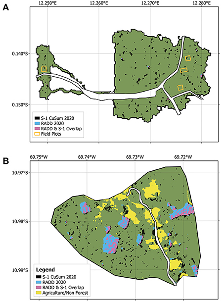
Figure 11. Comparison between RADD Alerts (blue) (Reiche et al., 2021) and CuSum change detection algorithm (black) for disturbances in the year 2020 in our study areas in (A) Gabon and (B) Peru. Overlapping areas between the two products are color coded in pink. The non-forest mask in (B) is the product of a land cover classification produced by the authors using PlanetScope 3m resolution imagery from 16th July 2019.

4. Discussion

This study provides the first ground truth validation of the CuSum change detection algorithm. This was successfully tested over tropical rainforests located in the Amazon (Peru) and Central Africa (Gabon). Highly accurate information on the spatiotemporal distribution and the magnitude of forest loss was derived by a combination of field-measured UAV LiDAR, TLS, and forest inventory data. We have adopted a single change metric, the maximum value of the CuSum distribution, to map the location, timing, and magnitude of forest canopy loss. The sites selected for this study presented different degrees of disturbances, from individual tree removal to clear cuts and forest fragmentation in proximity of an inhabited area. The CuSum algorithm was able to detect the full spectrum of the disturbances, with a 78% probability of detection over the study site in Gabon and 65% probability of detection over the study site in Peru, for patches as small as 0.01 ha in size and canopy disturbances of 10 m and greater in vertical drop, including variations in the understory vegetation. The probability of detection increased to 100% in Gabon and 90% in Peru when considering detections equal or greater than 0.05 ha in size. Sentinel-1 data analyzed with this algorithm exceeded our expectations in its ability to estimate the timing of disturbance events, such as selective logging in our study plots early in 2020 vs. the more widespread selective logging in the forest concession at the end of the same year (Figure 7A).

4.1. Reproducibility and generality

The results of this study indicate that the CuSum method is an effective, simple, and highly reproducible tool for monitoring forest structure dynamics, even in the case of low-intensity logging. Forest monitoring systems relying on optical imagery, such as the GFW Alerts (Hansen et al., 2016) and DETER in Brazil (Shimabukuro et al., 2006), are inherently limited by cloud coverage, which hampers the possibility of capturing the full extent of forest loss in tropical regions. Building on the freely available, temporally dense, and cloud-penetrating Sentinel-1 dataset, the CuSum method is suitable for mapping disturbances in a continuous manner and at pan-tropical scales (Ruiz-Ramos et al., 2020; Hethcoat et al., 2021). In particular, the algorithm was successfully tested in two contrasting tropical forest ecosystems, the Amazon and Central Africa rainforests, which greatly differ in species composition and stand structure. In both locations we used experimental data from UAV LiDAR to calibrate the algorithm to distinguish intact forest from disturbed forest, thus setting an empirical threshold on the change metric. Interestingly, we have found that the 95th percentile of the CuSum maximum distribution approximately corresponds to the value of this empirical threshold (Figure S4). This opens the possibility of extending the proposed method beyond the test sites, even in the absence of in-situ measurements of forest canopy loss. The detection accuracy of this approach needs to be further explored, and the analysis scaled to the regional level to evaluate the variability of the threshold in response to differences in forest structure and topography.

In terms of disturbance characteristics, the CuSum method was able to detect a variety of disturbance events ranging from small-scale logging for commercial timber extraction (e.g., in Gabon) to large area deforestation for subsequent agricultural use (e.g., near the village in Peru). This classification is only possible thanks to our detailed, first-hand knowledge of the study sites, as the CuSum method on its own does not provide any information on the underlying causes of the disturbance. For example, tree mortality, wind, and other natural factors are the likely causes of canopy losses observed in the area surrounding our field plots in Peru (Figure 6B). In this case, the location and size of the disturbance clusters does not provide any information on the nature of these events, making it difficult to distinguish them from the anthropogenic disturbances that occurred within and in close proximity of the study plots. There are cases where it is possible to identify the nature of the disturbances by looking at the shape and location of the clusters. For example, new logging roads and crop fields are easily recognizable, as they arrange themselves in geometric patterns and are usually connected to other features in the landscape. A caveat on scaling this methodology on a larger area is that automatic remote sensing approaches may not be sufficient for an accurate classification: fieldwork, knowledge of the study area, and image interpretation are still crucial to fully understand the dynamics on the ground (Myers, 2010; Reams et al., 2010; Beuchle et al., 2021).

4.1.1. Location accuracy vs. timely event detection

The majority of fine-scale disturbances in our study areas went undetected by the RADD product, which is currently the best SAR-based system for mapping forest disturbances across the tropics (Reiche et al., 2021). In our study site in Gabon (where RADD provides data for the year of the logging activities), RADD was able to detect only 2% of the disturbances measured by our reference map (7 RADD vs. 317 LiDAR detections)—as compared to 59% from CuSum (187 CuSum vs. 317 LiDAR detections)—missing all the selective logging in our core plots. However, we have not tested the performance of the CuSum method for NRT monitoring, which is the essential feature of the RADD Alert system. The potential of CuSum analysis for NRT has already been proposed by the literature (Ruiz-Ramos et al., 2020). As the success of the CuSum algorithm is ultimately linked to constructing an adequate picture of the pre- and post-disturbance trend, there is an intrinsic limitation on the minimum number of images required for capturing the point-wise change that we classify as a detection. In this study, we have tested the CuSum method on time series acquired using a repeat-track orbit and a descending acquisition mode, using a minimum of 12 months (≈ 30 images) for building the pre-disturbance dataset and a minimum of 6 months (≈ 15 images) for the post-disturbance trend. Enhancing NRT performance, for example by reducing the amount of images required to build the post-disturbance dataset, may also reduce the number of detections. Compared to the RADD system, the CuSum method is able to detect disturbances as small as 0.01 ha in size (as compared to 0.1 ha, the minimum mapping unit for RADD) and can provide accurate information on time and magnitude of the disturbance events. On the other hand, the intrinsic latency of the method may not make it suitable for NRT detections. However, while future work should explore the possibility of enhancing NRT capability of the CuSum algorithm, the two systems can complement each other in terms of usage and applications. For example, while RADD may be appropriate for mapping activities that require immediate intervention (such as illegal logging), the CuSum methodology can be used for building yearly maps of forest loss, providing more accurate figures on time and magnitude of the disturbance events for long-term monitoring and reporting purposes.

4.1.2. Potential for biomass change estimates

In this study, we explored for the first time the relationship between the CuSum method and forest physical parameters, using the same metric that was adopted for mapping location and time of the disturbances. A statistically significant relationship (R² = 0.95 and p < 0.001) was found between the CuSum maximum and field-measured AGB loss percentages at a 1 ha scale (Figure 9). The spread of R_{sum_max} values for the assumed 0% and 100% ΔAGB plots in Figure 9 is evidence that the plots were not field-inventoried, and hence the associated value of ΔAGB may be inaccurate. For example, plots that are not selectively logged will still experience small variations in forest biomass due to natural tree mortality. Despite the underlying noise, these plots adds evidence to the assumption that the magnitude of R_{sum_max} is directly correlated to the amount of biomass removed. Hence, a pan-tropical linear model was used for directly deriving maps of forest biomass change with values ranging from 0% (intact forest) to 100% change (deforestation). The maps show different levels of disturbance compared to each other, which can be explained by the distinctive characteristics of the two sites. In Gabon, this region is scarcely populated, the main human settlement being the village of Ivindo in the western corner, which is also the site of Rougier's logging camp. The rest of the area is dominated by a dense canopy cover and is largely part of Rougier's forest concession, bordered east by Ivindo National Park and south by the Ogooué River. Here, timber is logged on a rotational basis and at low-intensities, according to FSC-certified protocols. Limited patches of deforestation are observed in proximity of the village, likely caused by the logging camp activities, as it was observed during the field campaigns. The area in Peru, on the other hand, is characterized by a higher human presence, especially concentrated in and the around the town of Iñapari and the Bélgica village, with small, isolated households scattered along the Acre River, which marks the border between Peru and Brazil. Consistent patterns of forest disturbance are visible in proximity of human settlements and bordering grasslands and agricultural fields, indicating agricultural expansion into the forest fringes. Most of these patterns are concentrated along transport infrastructures, namely the Acre River and the road connecting Iñapari to Bélgica. However, land use in Bélgica's territory (dashed black line) is regulated and, with the exception of the area around the village which is allocated to agricultural/urban use, it is mainly divided between a protected area and a forest concession for low-intensity timber extraction. Indeed, the biomass change map shows a clear demarcation in land use as soon as the road from Iñapari enters Bélgica's territory (Figure 10B). These observations are in line with findings from previous studies (Hirschmugl et al., 2020), which report similar patterns of forest disturbances in test sites located in the forests of Peru and Gabon.

A lack of ground measurements of forest biomass change in these areas combined with the absence of remote sensing products on AGB loss figures makes it difficult to validate these maps; however, at least for deforestation rates (AGB Loss = 100%), we can compare our findings with the GFW dataset (Hansen et al., 2016). In Peru, where forest disturbance is more widespread, we found a 61% overlap between the two maps, for detections covering ≈1% of the overall study area. The overlap increased to 90% when the CuSum map included pixels containing at least 50% biomass loss (Figure S3). Different spatial resolutions—30 × 30 m for the original GFW dataset, resampled to 100 × 100 m for comparing purposes—and the geometric incongruency of the two sensors (Landsat for GFW vs. Sentinel-1 for our study) are limiting factors for this analysis, where we may be excluding pixels that are very close but not intersecting. The final result still shows the ability of the CuSum algorithm to correctly locate the deforestation areas, presenting itself as a complementary tool to optical datasets for monitoring forest loss.

4.1.3. Limitations and future work

This study presents a first empirical application of the CuSum method, showing the potential of this technique for future forest disturbance mapping. On the other hand, this work opens up further trajectories of research, which can refine the methodology presented here, or even translate the analysis to other areas of investigation where change detection methods are required.

In this work, we have only considered the co-polarized backscatter (VV), which is generally sensitive to surface or double-bounce scattering mechanisms between radar signal and measured target. On the other hand, the cross-polarized channel (VH) is useful to describe variations in the presence of multiple-bounce or volume scattering. A combination of co- and cross-polarized backscatter, such as the ratio of VH and VV backscatter, should be more sensitive to vegetation dynamics (Veloso et al., 2017). Ygorra et al. (2021) has concluded that the best detection of vegetation cover change is achieved when combining both VV and VH; hence, future work should look at adding information from the VH channel, and possibly testing the detection ability of the combined ratio (VH/VV). The number of detections may be further increased by combining both the positive and negative CuSum curves that were shown in Figure 5. Such analysis may also improve our understanding of the scattering mechanisms at play in the presence of the change event. In this study, we have focused on the detection of a single change event over the entire period of observation. Nonetheless, a pixel may experience multiple disturbances, especially over the course of a multi-year analysis. For example, different waves of selective logging may occur within the same pixel, leading to a clearing event or to conversion into another land use. A complete analysis of the disturbance trends should include the detection of these secondary change points. This can be achieved by dividing the time series before and after R_{sum_max} and repeating the analysis until the value of R_{sum_max} falls below the selected threshold.

Another direction of work should then focus on generalizing the algorithm beyond the availability of in-situ measurements, by improving the thresholding procedure and decoupling it from the empirical data, for example by using statistical inference as proposed here, or more advanced time series techniques. Furthermore, the ability to retrieve biomass loss estimates directly from the change metric should be refined by adding more ground measurements to the regression model covering the entire spectrum of forest disturbance rates; and by using ground measurements, including the low-magnitude AGB loss, to validate the final product. The output should be validated in different areas and for different magnitudes of biomass change, especially for the low-intensity variations. Adding calibration data at finer resolutions (< 1 ha), for example using the LiDAR metrics, would allow to retrieve estimates of biomass change potentially even at the original 10 m scale, providing better results for local and regional assessments of forest health.

Since the CuSum technique is essentially a change detection method, it can be exploited for monitoring other types of abrupt or sustained changes in land use, such as crop dynamics, floods, and soil cover changes (Ruiz-Ramos et al., 2020; Ygorra et al., 2021). It can be similarly implemented on other SAR-based datasets at different wavelengths, such as the upcoming ESA's Biomass P-band mission, NASA's NISAR L/S-band, and JAXA's ALOS-4 L-band, all planned for launch in 2023. Due to the nature of the field measurements, the analysis in this paper was limited to measures of forest loss; however, this does not exclude the possibility of using the same method for mapping forest regrowth. A very interesting line of research would be to observe the behavior of the CuSum distribution in the case of positive changes in stand volume or in canopy height, expanding the analysis to include estimates of forest gain, which are still excluded from current SAR-based monitoring systems.

5. Conclusions

This study presents a simple and effective methodology for detecting fine-scale disturbances in dense and multistoried tropical forests. A single metric based on the CuSums of VV-polarized Sentinel-1 time series was used to retrieve location, time, and magnitude of the disturbances. The results of the change detection algorithm were tested on highly detailed, in situ measurements of forest canopy loss retrieved with a combination of UAV LiDAR, TLS, and field inventory surveys, in the two distinct tropical forests located in Gabon and Peru. The probability of detection for this new method was 78% in the test site in Gabon and 65% in the test site in Peru, for disturbances as small as 0.01 ha in size and for drops in tree height as low as 10 m, including changes in understory vegetation. The timing of the detections matched the time when selective logging was carried out the field plots; in the wider concessions, it was consistent with the patterns of disturbances of the two test sites. The algorithm presented here was able to capture different intensities of forest degradation and deforestation, outdoing other forest monitoring tools such as the SAR-based RADD system and the Landsat-based GFW tool in capturing finer and more widespread tropical forest disturbances. In addition to other forest monitoring systems, the methodology outlined in this paper has the potential of retrieving the magnitude of the disturbance. A correlation between the change metric and biomass change was found with R² = 0.95 and R² = 0.83 for canopy height loss. Given the global coverage and free availability of Sentinel-1 data, the approach can be generalized to the regional scale and potentially used to quantify other types of forest dynamics, such as forest regrowth.

Data availability statement

The underlying data is available from the University of Edinburgh DataShare service (https://datashare.ed.ac.uk/handle/10283/4116). The script performing the change detection analysis is available on GitHub (https://github.com/chiaquino/S1_CuSum).

Author contributions

CA: conceptualization, software, validation, formal analysis, writing—original draft preparation, and visualization. EM: project administration and funding acquisition. CA and EM: methodology. CA, IM, HC, BP, MO, AM, CD, MT, PG, and FM: investigation. AB, MD, SM, BP, MT, PG, and FM: resources. CA, IM, HC, and AB: data curation. CA, EM, and MD: writing—review and editing. EM and MD: supervision. All authors reviewed the manuscript.

Funding

This research was funded by a European Research Council Starting Grant awarded to EM (The Tropical Forest Degradation Experiment—FODEX: 757526). MD was funded for capital equipment by UCL Geography and the UK NERC National Centre for Earth Observation.

Acknowledgments

We wish to thank La Comunidad Nativa de Bélgica for allowing us to conduct this research on their land and for their generous hospitality; the NGO AIDER for offering their invaluable help with preparation and field logistics with the Peruvian campaigns; Prof. Eric Cosio and Dr. Norma Salinas from the Pontificia Universidad Católica del Perú for their assistance with customs and logistics. We would like to thank the staff of Rougier Gabon, including Evanillho Téodoro Muaño Bondjale and Aimé Manfoumbi, for hosting us in Ivindo and supporting us with our fieldwork. We are very grateful to Alfred Ngomanda from the Centre National de la Recherche Scientifique et Technologique (CENAREST); to the Agence Nationale des Parcs Nationaux (ANPN); to Le Ministère des Eaux, des Forets, de la Mer, de l'Environnement du Gabon, and to the Institut de Recherche en Ecologie Tropicale (IRET) for their invaluable support to our research in Gabon. This research would have not been possible without the work of the field assistants. In particular, we would like to thank Luis Miguel Álvarez Mayorga, Roxana Sacatuma Cruz, José Sánchez Tintaya, Arturo Aspajo López, Leoncio Aspajo Lopez, Luis López Chapiama, and Kenny López Batista for the assistance in Peru; Joseph Amelim Boukandja and the community of Ivindo for assisting us with the fieldwork in Gabon.

Conflict of interest

Author FM was employed by Cotecmi S.A.C.

The remaining authors declare that the research was conducted in the absence of any commercial or financial relationships that could be construed as a potential conflict of interest.

Publisher's note

All claims expressed in this article are solely those of the authors and do not necessarily represent those of their affiliated organizations, or those of the publisher, the editors and the reviewers. Any product that may be evaluated in this article, or claim that may be made by its manufacturer, is not guaranteed or endorsed by the publisher.

Supplementary material

The Supplementary Material for this article can be found online at: https://www.frontiersin.org/articles/10.3389/ffgc.2022.1018762/full#supplementary-material

Table S1. Comparison between Aboveground Biomass change (ΔAGB) figures of eight 1-ha selectively logged plots located in Gabon (G) and Peru (P), where the AGB of the logged trees is calculated either using an allometric equation (Allometric ΔAGB) or Terrestrial Laser Scanning data (TLS ΔAGB). Allometric ΔAGB is calculated as the difference in AGB between the first and second inventory. TLS ΔAGB is the sum of the TLS volumes for the logged trees and the difference in AGB between the first and second inventory for the unlogged trees. Standard errors are reported in parentheses.

Figure S1. Comparison between Aboveground Biomass (AGB) values derived using allometric equations and AGB values derived from Terrestrial Laser Scanning (TLS) measurements for the logged trees in Gabon (blue triangles) and Peru (red circles).

Figure S2. Maps of the CuSum spatial results for the study in area in Gabon, showing the location of the detections from the CuSum method (red), the results from the LiDAR reference map (blue) and the overlaps between CuSum and LiDAR detections, for CuSum clusters of increasing size: (A) CuSum clusters ≥ 0.01 ha; (B) CuSum clusters ≥ 0.02 ha; (C) CuSum clusters ≥ 0.05 ha; (D) CuSum clusters ≥ 0.1 ha.

Figure S3. Comparing the GFW Tree Cover Loss product and the CuSum-derived aboveground biomass (AGB) loss map for the Peru test site, at different threshold of AGB loss: (A) AGB Loss = 100%, (B) CuSum AGB Loss > 80%; (C) CuSum AGB Loss > 60%; (D) CuSum AGB Loss > 50%.

Figure S4. Comparison of thresholding procedures for change detection. 1) Thresholding using UAV LiDAR data to calculate the value minimising both False Positive (FP) and False Negative (FN) detections yields R_{sum_max} = 33 for Gabon (top left) and R_{sum_max} = 36 for Peru (top right). 2) Thresholding using the 95th percentile of the R_{sum_max} distribution gives a value of R_{sum_max} = 31 for Gabon (bottom left) and R_{sum_max} = 42 for Peru (bottom right).

Figure S5. LiDAR vertical profile of the field site in Gabon, showing the presence of multi-storied forest canopies.

References

Achard, F., Stibig, H.-J., Eva, H. D., Lindquist, E. J., Bouvet, A., Arino, O., et al. (2010). Estimating tropical deforestation from earth observation data. Carbon Manage. 1, 271–287. doi: 10.4155/cmt.10.30

CrossRef Full Text | Google Scholar

Adler, R. F., Huffman, G. J., Chang, A., Ferraro, R., Xie, P.-P., Janowiak, J., et al. (2003). The version-2 global precipitation climatology project (GPCP) monthly precipitation analysis (1979present). J. Hydrometeorol. 4, 1147–1167. doi: 10.1175/1525-7541(2003)004<1147:TVGPCP>2.0.CO;2

PubMed Abstract | CrossRef Full Text | Google Scholar

Asiyanbi, A. P., Arhin, A. A., and Isyaku, U. (2017). REDD+ in West Africa: politics of design and implementation in Ghana and Nigeria. Forests 8:78. doi: 10.3390/f8030078

CrossRef Full Text | Google Scholar

Asner, G. P., Keller, M., Pereira Jr., R, Zweede, J. C., and Silva, J. N. M. (2004). Canopy damage and recovery after selective logging in Amazonia: field and satellite studies. Ecol. Appl. 14, 280–298. doi: 10.1890/01-6019

CrossRef Full Text | Google Scholar

Ballre, M., Bouvet, A., Mermoz, S., Le Toan, T., Koleck, T., Bedeau, C., et al. (2021). SAR data for tropical forest disturbance alerts in French Guiana: benefit over optical imagery. Remote Sens. Environ. 252:112159. doi: 10.1016/j.rse.2020.112159

CrossRef Full Text | Google Scholar

Bayrak, M. M., and Marafa, L. M. (2016). Ten years of REDD+: a critical review of the impact of REDD+ on forest-dependent communities. Sustainability 8:620. doi: 10.3390/su8070620

CrossRef Full Text | Google Scholar

BBurt, A., Boni Vicari, M., da Costa, A. C. L., Coughlin, I., Meir, P., Rowland, L., et al. (2021). New insights into large tropical tree mass and structure from direct harvest and terrestrial lidar. R. Soc. Open Sci. 8:201458. doi: 10.1098/rsos.201458

PubMed Abstract | CrossRef Full Text | Google Scholar

Beuchle, R., Achard, F., Bourgoin, C., Vancutsem, C., Eva, H., and Follador, M. (2021). Deforestation and Forest Degradation in the Amazon - Status and Trends up to Year 2020. JRC Publications Repository.

Google Scholar

Bouvet, A., Mermoz, S., Ballére, M., Koleck, T., and Le Toan, T. (2018a). Use of the SAR shadowing effect for deforestation detection with Sentinel-1 time series. Remote Sens. 10:1250. doi: 10.3390/rs10081250

CrossRef Full Text | Google Scholar

Bouvet, A., Mermoz, S., Le Toan, T., Villard, L., Mathieu, R., Naidoo, L., et al. (2018b). An above-ground biomass map of African savannahs and woodlands at 25m resolution derived from ALOS PALSAR. Remote Sens. Environ. 206, 156–173. doi: 10.1016/j.rse.2017.12.030

CrossRef Full Text | Google Scholar

Bullock, E. L., Woodcock, C. E., and Olofsson, P. (2020). Monitoring tropical forest degradation using spectral unmixing and Landsat time series analysis. Remote Sens. Environ. 238:110968. doi: 10.1016/j.rse.2018.11.011

CrossRef Full Text | Google Scholar

Burga Cahuana, C. (2013). Participation and Representation: REDD+ in the Native Communities of Belgica and Infierno in the Peruvian Amazon. Master's Thesis, University of Illinois at Urbana-Champaign.

Google Scholar

Burt, A., Disney, M., and Calders, K. (2019). Extracting individual trees from lidar point clouds using treeseg. Methods Ecol. Evol. 10, 438–445. doi: 10.1111/2041-210X.13121

PubMed Abstract | CrossRef Full Text | Google Scholar

Caballero Espejo, J., Messinger, M., Román–Dañobeytia, F., Ascorra, C., Fernandez, L. E., and Silman, M. (2018). Deforestation and forest degradation due to gold mining in the Peruvian amazon: a 34-year perspective. Remote Sens. 10:1903. doi: 10.3390/rs10121903

CrossRef Full Text | Google Scholar

Calders, K., Newnham, G., Burt, A., Murphy, S., Raumonen, P., Herold, M., et al. (2015). Nondestructive estimates of above-ground biomass using terrestrial laser scanning. Methods Ecol. Evol. 6, 198–208. doi: 10.1111/2041-210X.12301

CrossRef Full Text | Google Scholar

Carstairs, H., Mitchard, E. T. A., McNicol, I., Aquino, C., Burt, A., Ebanega, M. O., et al. (2022). An effective method for InSAR mapping of tropical forest degradation in hilly areas. Remote Sens. 14:452. doi: 10.3390/rs14030452

CrossRef Full Text | Google Scholar

Castro, M. C., Baeza, A., Codeço, C. T., Cucunubá, Z. M., Dal'Asta, A. P., Leo, G. A. D., et al. (2019). Development, environmental degradation, and disease spread in the Brazilian Amazon. PLOS Biol. 17:e3000526. doi: 10.1371/journal.pbio.3000526

PubMed Abstract | CrossRef Full Text | Google Scholar

Chave, J. (2014). Generic Tree Allometric Models. < Available online at: https://chave.ups-tlse.fr/pantropical_allometry.htm (accessed January 13, 2021). doi: 10.5585/riae.v13i4.2179

CrossRef Full Text | Google Scholar

Chave, J., Coomes, D., Jansen, S., Lewis, S. L., Swenson, N. G., and Zanne, A. E. (2009). Towards a worldwide wood economics spectrum. Ecol. Lett. 12:351–366. doi: 10.1111/j.1461-0248.2009.01285.x

PubMed Abstract | CrossRef Full Text | Google Scholar

Chave, J., RjouMchain, M., Brquez, A., Chidumayo, E., Colgan, M. S., Delitti, W. B. C., et al. (2014). Improved allometric models to estimate the aboveground biomass of tropical trees. Glob. Chang. Biol. 20, 3177–3190. doi: 10.1111/gcb.12629

PubMed Abstract | CrossRef Full Text | Google Scholar

D'Almeida, C., Vörösmarty, C. J., Hurtt, G. C., Marengo, J. A., Dingman, S. L., and Keim, B. D. (2007). The effects of deforestation on the hydrological cycle in Amazonia: a review on scale and resolution. Int. J. Climatol. 27, 633–647. doi: 10.1002/joc.1475

CrossRef Full Text | Google Scholar

Deutscher, J., Gutjahr, K., Perko, R., Raggam, H., Hirschmugl, M., and Schardt, M. (2017). “Humid tropical forest monitoring with multi-temporal L-, C- and X-band SAR data,” in 2017 9th International Workshop on the Analysis of Multitemporal Remote Sensing Images (MultiTemp) (Bruges), 1–4.

Google Scholar

Diringer, S. E., Berky, A. J., Marani, M., Ortiz, E. J., Karatum, O., Plata, D. L., et al. (2020). Deforestation due to artisanal and small-scale gold mining exacerbates soil and mercury mobilization in Madre de Dios, Peru. Environ. Sci. Technol. 54, 286–296. doi: 10.1021/acs.est.9b06620

PubMed Abstract | CrossRef Full Text | Google Scholar

FAO (2020). Global Forest Resources Assessment 2020: Key findings. Rome: FAO.

Google Scholar

Federici, S., Tubiello, F. N., Salvatore, M., Jacobs, H., and Schmidhuber, J. (2015). New estimates of CO2 forest emissions and removals: 1990–2015. For. Ecol. Manage. 352,89–98. doi: 10.1016/j.foreco.2015.04.022

CrossRef Full Text | Google Scholar

Giam, X. (2017). Global biodiversity loss from tropical deforestation. Proc. Nat. Acad. Sci. USA 114, 5775–5777. doi: 10.1073/pnas.1706264114

PubMed Abstract | CrossRef Full Text | Google Scholar

Gonzalez de Tanago, J., Lau, A., Bartholomeus, H., Herold, M., Avitabile, V., Raumonen, P., et al. (2018). Estimation of above-ground biomass of large tropical trees with terrestrial LiDAR. Methods Ecol. Evol. 9, 223–234. doi: 10.1111/2041-210X.12904

CrossRef Full Text | Google Scholar

Google Earth Engine (2021). Sentinel-1 Algorithms. Available online at: https://developers.google.com/earth-engine/guides/sentinel1 (accessed June 15, 2022).

Google Scholar

Gorelick, N., Hancher, M., Dixon, M., Ilyushchenko, S., Thau, D., and Moore, R. (2017). Google Earth Engine: Planetary-scale geospatial analysis for everyone. Remote Sens. Environ. 202, 18–27. doi: 10.1016/j.rse.2017.06.031

CrossRef Full Text | Google Scholar

Hansen, M. C., Krylov, A., Tyukavina, A., Potapov, P. V., Turubanova, S., Zutta, B., et al. (2016). Humid tropical forest disturbance alerts using Landsat data. Environ. Res. Lett. 11:034008. doi: 10.1088/1748-9326/11/3/034008

CrossRef Full Text | Google Scholar

Hansen, M. C., Potapov, P. V., Moore, R., Hancher, M., Turubanova, S. A., Tyukavina, A., et al. (2013). High-resolution global maps of 21st-century forest cover change. Science 342, 850–853. doi: 10.1126/science.1244693

PubMed Abstract | CrossRef Full Text | Google Scholar

Henders, S., Persson, U. M., and Kastner, T. (2015). Trading forests: land-use change and carbon emissions embodied in production and exports of forest-risk commodities. Environ. Res. Lett. 10:125012. doi: 10.1088/1748-9326/10/12/125012

CrossRef Full Text | Google Scholar

Herold, M., Román-Cuesta, R. M., Mollicone, D., Hirata, Y., Van Laake, P., Asner, G. P., et al. (2011). Options for monitoring and estimating historical carbon emissions from forest degradation in the context of REDD+. Carbon Balance Manag. 6:13. doi: 10.1186/1750-0680-6-13

PubMed Abstract | CrossRef Full Text | Google Scholar

Hethcoat, M. G., Carreiras, J. M. B., Edwards, D. P., Bryant, R. G., and Quegan, S. (2021). Detecting tropical selective logging with C-band SAR data may require a time series approach. Remote Sens. Environ. 259:112411. doi: 10.1016/j.rse.2021.112411

CrossRef Full Text | Google Scholar

Hirschmugl, M., Deutscher, J., Sobe, C., Bouvet, A., Mermoz, S., and Schardt, M. (2020). Use of SAR and optical time series for tropical forest disturbance mapping. Remote Sens. 12:727. doi: 10.3390/rs12040727

PubMed Abstract | CrossRef Full Text | Google Scholar

Hoang, N. T., and Kanemoto, K. (2021). Mapping the deforestation footprint of nations reveals growing threat to tropical forests. Nat. Ecol. Evol. 5, 845–853. doi: 10.1038/s41559-021-01417-z

PubMed Abstract | CrossRef Full Text | Google Scholar

Houghton, R. A., House, J. I., Pongratz, J., Werf, G. R. v. d., DeFries, R. S., Hansen, M. C., et al. (2012). Carbon emissions from land use and land-cover change. Biogeosciences 9, 5125–5142. doi: 10.5194/bg-9-5125-2012

PubMed Abstract | CrossRef Full Text | Google Scholar

Imhoff, M. L. (1995). Radar backscatter and biomass saturation: ramifications for global biomass inventory. IEEE Trans. Geosci. Remote Sens. 33, 511–518. doi: 10.1109/36.377953

CrossRef Full Text | Google Scholar

Joshi, N., Baumann, M., Ehammer, A., Fensholt, R., Grogan, K., Hostert, P., et al. (2016). A Review of the application of optical and radar remote sensing data fusion to land use mapping and monitoring. Remote Sens. 8:70. doi: 10.3390/rs8010070

PubMed Abstract | CrossRef Full Text | Google Scholar

Joshi, N., Mitchard, E. T., Woo, N., Torres, J., Moll-Rocek, J., Ehammer, A., et al. (2015). Mapping dynamics of deforestation and forest degradation in tropical forests using radar satellite data. Environ. Res. Lett. 10:034014. doi: 10.1088/1748-9326/10/3/034014

CrossRef Full Text | Google Scholar

Joshi, N., Mitchard, E. T. A., Brolly, M., Schumacher, J., Fernández-Landa, A., Johannsen, V. K., et al. (2017). Understanding “saturation” of radar signals over forests. Sci. Rep. 7:3505. doi: 10.1038/s41598-017-03469-3

PubMed Abstract | CrossRef Full Text | Google Scholar

Kellndorfer, J. (2019). “Using SAR data for mapping deforestation and forest degradation,” in The SAR Handbook. Comprehensive Methodologies for Forest Monitoring and Biomass Estimation, eds A. I. Flores-Anderson, K. E. Herndon, R. B. Thapa, and E. Cherrington (Hunstville, AL: Servir Global), 65–79.

Google Scholar

Le Toan, T., Beaudoin, A., Riom, J., and Guyon, D. (1992). Relating forest biomass to SAR data. IEEE Trans. Geosci. Remote Sens. 30, 403–411. doi: 10.1109/36.134089

CrossRef Full Text | Google Scholar

Le Toan, T., Quegan, S., Woodward, I., Lomas, M., Delbart, N., and Picard, G. (2004). Relating radar remote sensing of biomass to modelling of forest carbon budgets. Clim. Change 67, 379–402. doi: 10.1007/s10584-004-3155-5

CrossRef Full Text | Google Scholar

Lewis, S. L., Phillips, O. L., Sheil, D., Vinceti, B., Baker, T. R., Brown, S., et al. (2004). Tropical forest tree mortality, recruitment and turnover rates: calculation, interpretation and comparison when census intervals vary. J. Ecol. 92, 929–944. doi: 10.1111/j.0022-0477.2004.00923.x

CrossRef Full Text | Google Scholar

Lohberger, S., Stängel, M., Atwood, E. C., and Siegert, F. (2018). Spatial evaluation of Indonesia's 2015 fire-affected area and estimated carbon emissions using Sentinel-1. Glob. Chang. Biol. 24, 644–654. doi: 10.1111/gcb.13841

PubMed Abstract | CrossRef Full Text | Google Scholar

Manly, B. F., and Mackenzie, D. I. (2003). CUSUM environmental monitoring in time and space. Environ. Ecol. Stat. 10, 231–247. doi: 10.1023/A:1023682426285

CrossRef Full Text | Google Scholar

Manogaran, G., and Lopez, D. (2018). Spatial cumulative sum algorithm with big data analytics for climate change detection. Comput. Electr. Eng. 65, 207–221. doi: 10.1016/j.compeleceng.2017.04.006

CrossRef Full Text | Google Scholar

Markham, K. E., and Sangermano, F. (2018). Evaluating wildlife vulnerability to mercury pollution from artisanal and small-scale gold mining in Madre de Dios, Peru. Trop. Conserv. Sci. 11:1940082918794320. doi: 10.1177/1940082918794320

CrossRef Full Text | Google Scholar

Matricardi, E. A. T., Skole, D. L., Costa, O. B., Pedlowski, M. A., Samek, J. H., and Miguel, E. P. (2020). Long-term forest degradation surpasses deforestation in the Brazilian Amazon. Science 369, 1378–1382. doi: 10.1126/science.abb3021

PubMed Abstract | CrossRef Full Text | Google Scholar

McAfee, K. (2012). The contradictory logic of global ecosystem services markets. Dev. Change 43, 105–131. doi: 10.1111/j.1467-7660.2011.01745.x

PubMed Abstract | CrossRef Full Text | Google Scholar

McNicol, I. M., Mitchard, E. T. A., Aquino, C., Burt, A., Carstairs, H., Dassi, C., et al. (2021). To what extent can UAV photogrammetry replicate UAV LiDAR to determine forest structure? A test in two contrasting tropical forests. J. Geophys. Res. Biogeosci. 126:e2021JG006586. doi: 10.1029/2021JG006586

CrossRef Full Text | Google Scholar

Medjibe, V. P., Putz, F. E., and Romero, C. (2013). Certified and uncertified logging concessions compared in gabon: changes in stand structure, tree species, and biomass. Environ. Manage. 51, 524–540. doi: 10.1007/s00267-012-0006-4

PubMed Abstract | CrossRef Full Text | Google Scholar

Mermoz, S., Réjou-Méchain, M., Villard, L., Le Toan, T., Rossi, V., and Gourlet-Fleury, S. (2015). Decrease of L-band SAR backscatter with biomass of dense forests. Remote Sens. Environ. 159, 307–317. doi: 10.1016/j.rse.2014.12.019

CrossRef Full Text | Google Scholar

Mitchard, E. T. A. (2018). The tropical forest carbon cycle and climate change. Nature 559, 527–534. doi: 10.1038/s41586-018-0300-2

PubMed Abstract | CrossRef Full Text | Google Scholar

Mitchard, E. T. A., Saatchi, S. S., Lewis, S. L., Feldpausch, T. R., Gerard, F. F., Woodhouse, I. H., et al. (2011a). Comment on ‘A first map of tropical Africa's above-ground biomass derived from satellite imagery'. Environ. Res. Lett. 6:049001. doi: 10.1088/1748-9326/6/4/049001

CrossRef Full Text | Google Scholar

Mitchard, E. T. A., Saatchi, S. S., Lewis, S. L., Feldpausch, T. R., Woodhouse, I. H., Sonk, B., et al. (2011b). Measuring biomass changes due to woody encroachment and deforestation/degradation in a forest–savanna boundary region of central Africa using multi-temporal L-band radar backscatter. Remote Sens. Environ. 115, 2861–2873. doi: 10.1016/j.rse.2010.02.022

CrossRef Full Text | Google Scholar

Myers, A. (2010). Camp Delta, Google Earth and the ethics of remote sensing in archaeology. World Archaeol. 42, 455–467. doi: 10.1080/00438243.2010.498640

CrossRef Full Text | Google Scholar

Nielsen, T. D. (2014). The role of discourses in governing forests to combat climate change. Int. Environ. Agreem. Polit. Law Econ. 14, 265–280. doi: 10.1007/s10784-013-9223-4

CrossRef Full Text | Google Scholar

Nunes, L. J. R., Meireles, C. I. R., Pinto Gomes, C. J., and Almeida Ribeiro, N. M. C. (2020). Forest contribution to climate change mitigation: management oriented to carbon capture and storage. Climate 8:21. doi: 10.3390/cli8020021

CrossRef Full Text | Google Scholar

Page, E. S. (1955). A test for a change in a parameter occurring at an unknown point. Biometrika 42, 523–527. doi: 10.1093/biomet/42.3-4.523

CrossRef Full Text | Google Scholar

Pan, Y., Birdsey, R. A., Phillips, O. L., and Jackson, R. B. (2013). The structure, distribution, and biomass of the world's forests. Annu. Rev. Ecol. Evol. Syst. 44, 593–622. doi: 10.1146/annurev-ecolsys-110512-135914

CrossRef Full Text | Google Scholar

Pendrill, F., Persson, U. M., Godar, J., and Kastner, T. (2019a). Deforestation displaced: trade in forest-risk commodities and the prospects for a global forest transition. Environ. Res. Lett. 14:055003. doi: 10.1088/1748-9326/ab0d41

CrossRef Full Text | Google Scholar

Pendrill, F., Persson, U. M., Godar, J., Kastner, T., Moran, D., Schmidt, S., et al. (2019b). Agricultural and forestry trade drives large share of tropical deforestation emissions. Glob. Environ. Change 56, 1–10. doi: 10.1016/j.gloenvcha.2019.03.002

CrossRef Full Text | Google Scholar

Phillips, O., Baker, T., Feldpausch, T., and Brienen, R. (2001). “RAINFOR field manual for plot establishment and remeasurement,” in Pan-amazonia, 1st Edn. (The Royal Society), 1–30.

Google Scholar

Planet Team (2017). Planet Application Program Interface: In Space for Life on Earth. San Francisco, CA: Planet Team. Available online at: https://api.planet.com (accessed April 25, 2021).

Google Scholar

Poudel, M., Thwaites, R., Race, D., and Dahal, G. R. (2015). Social equity and livelihood implications of REDD+ in rural communities—a case study from Nepal. Int. J. Commons 9, 177–208. doi: 10.18352/ijc.444

CrossRef Full Text | Google Scholar

Poulsen, J. R., Koerner, S. E., Miao, Z., Medjibe, V. P., Banak, L. N., and White, L. J. T. (2017). Forest structure determines the abundance and distribution of large lianas in Gabon. Glob. Ecol. Biogeogr. 26, 472–485. doi: 10.1111/geb.12554

CrossRef Full Text | Google Scholar

Qin, Y., Xiao, X., Wigneron, J.-P., Ciais, P., Brandt, M., Fan, L., et al. (2021). Carbon loss from forest degradation exceeds that from deforestation in the Brazilian Amazon. Nat. Clim. Chang. 11, 442–448. doi: 10.1038/s41558-021-01026-5

CrossRef Full Text | Google Scholar

Raumonen, P., Kaasalainen, M., kerblom, M., Kaasalainen, S., Kaartinen, H., Vastaranta, M., et al. (2013). FFast automatic precision tree models from terrestrial laser scanner data. Remote Sens. 5, 491–520. doi: 10.3390/rs5020491

CrossRef Full Text | Google Scholar

Reams, G. A., Brewer, C. K., and Guldin, R. W. (2010). Remote sensing alone is insufficient for quantifying changes in forest cover. Proc. Nat. Acad. Sci. USA. 107:E145. doi: 10.1073/pnas.1008665107

PubMed Abstract | CrossRef Full Text | Google Scholar

Reiche, J., Hamunyela, E., Verbesselt, J., Hoekman, D., and Herold, M. (2018). Improving near-real time deforestation monitoring in tropical dry forests by combining dense Sentinel-1 time series with Landsat and ALOS-2 PALSAR-2. Remote Sens. Environ. 204, 147–161. doi: 10.1016/j.rse.2017.10.034

CrossRef Full Text | Google Scholar

Reiche, J., Mullissa, A., Slagter, B., Gou, Y., Tsendbazar, N.-E., Odongo-Braun, C., et al. (2021). Forest disturbance alerts for the Congo Basin using Sentinel-1. Environ. Res. Lett. 16:024005. doi: 10.1088/1748-9326/abd0a8

CrossRef Full Text | Google Scholar

Ruiz-Ramos, J., Marino, A., Boardman, C., and Suarez, J. (2020). Continuous forest monitoring using cumulative sums of Sentinel-1 timeseries. Remote Sens. 12:3061. doi: 10.3390/rs12183061

CrossRef Full Text | Google Scholar

Ryan, C. M., Hill, T., Woollen, E., Ghee, C., Mitchard, E., Cassells, G., et al. (2012). Quantifying small-scale deforestation and forest degradation in African woodlands using radar imagery. Glob. Change Biol. 18, 243–257. doi: 10.1111/j.1365-2486.2011.02551.x

CrossRef Full Text | Google Scholar

Shimabukuro, Y., Duarte, V., Anderson, L., Valeriano, D., Arai, E., Freitas, R., et al. (2006). Near real time detection of deforestation in the Brazilian Amazon using MODIS imagery. Ambi. Agua, 1, 37–47. doi: 10.4136/ambi-agua.4

CrossRef Full Text | Google Scholar

Shimizu, K., Ota, T., and Mizoue, N. (2019). Detecting forest changes using dense landsat 8 and Sentinel-1 time series data in tropical seasonal forests. Remote Sens. 11:1899. doi: 10.3390/rs11161899

CrossRef Full Text | Google Scholar

Silva, C. A., Guerrisi, G., Del Frate, F., and Sano, E. E. (2022). Near-real time deforestation detection in the Brazilian Amazon with Sentinel-1 and neural networks. Eur. J. Remote Sens. 55, 129–149. doi: 10.1080/22797254.2021.2025154

CrossRef Full Text | Google Scholar

Tarazona, Y., and Miyasiro-López, M. (2020). Monitoring tropical forest degradation using remote sensing. Challenges and opportunities in the Madre de Dios region, Peru. Remote Sens. Appl. Soc. Environ. 19:100337. doi: 10.1016/j.rsase.2020.100337

CrossRef Full Text | Google Scholar

Taylor, W. (2008). Change-Point Analysis: A Powerful New Tool For Detecting Changes. Taylor Enterprises, Inc.

Google Scholar

Turubanova, S., Potapov, P. V., Tyukavina, A., and Hansen, M. C. (2018). Ongoing primary forest loss in Brazil, Democratic Republic of the Congo, and Indonesia. Environ. Res. Lett. 13:074028. doi: 10.1088/1748-9326/aacd1c

CrossRef Full Text | Google Scholar

Vancutsem, C., Achard, F., Pekel, J.-F., Vieilledent, G., Carboni, S., Simonetti, D., et al. (2021). Long-term (1990–2019) monitoring of forest cover changes in the humid tropics. Sci. Adv. 7:eabe1603. doi: 10.1126/sciadv.abe1603

PubMed Abstract | CrossRef Full Text | Google Scholar

Vargas, C., Montalban, J., and Leon, A. A. (2019). Early warning tropical forest loss alerts in Peru using Landsat. Environ. Res. Commun. 1:121002. doi: 10.1088/2515-7620/ab4ec3

CrossRef Full Text | Google Scholar

Veloso, A., Mermoz, S., Bouvet, A., Le Toan, T., Planells, M., Dejoux, J.-F., et al. (2017). Understanding the temporal behavior of crops using Sentinel-1 and Sentinel-2-like data for agricultural applications. Remote Sens. Environ. 199, 415–426. doi: 10.1016/j.rse.2017.07.015

CrossRef Full Text | Google Scholar

Verhegghen, A., Eva, H., Ceccherini, G., Achard, F., Gond, V., Gourlet-Fleury, S., et al. (2016). The potential of Sentinel satellites for burnt area mapping and monitoring in the Congo Basin forests. Remote Sens. 8:986. doi: 10.3390/rs8120986

CrossRef Full Text | Google Scholar

Villard, L., and Borderies, P. (2007). Backscattering border effects for forests at C-band. PIERS Online 3, 731–735. doi: 10.2529/PIERS061006120418

CrossRef Full Text | Google Scholar

Virtanen, P., Gommers, R., Oliphant, T. E., Haberland, M., Reddy, T., Cournapeau, D., et al. (2020). SciPy 1.0: fundamental algorithms for scientific computing in Python. Nat. Methods 17, 261–272. doi: 10.1038/s41592-019-0686-2

PubMed Abstract | CrossRef Full Text | Google Scholar

Wilkes, P., Lau, A., Disney, M., Calders, K., Burt, A., Gonzalez de Tanago, J., et al. (2017). Data acquisition considerations for Terrestrial Laser Scanning of forest plots. Remote Sens. Environ. 196, 140–153. doi: 10.1016/j.rse.2017.04.030

CrossRef Full Text | Google Scholar

Woodhouse, I. H. (2017). Introduction to Microwave Remote Sensing. Boca Raton, FL: CRC Press. doi: 10.1201/9781315272573

CrossRef Full Text | Google Scholar

Ygorra, B., Frappart, F., Wigneron, J. P., Moisy, C., Catry, T., Baup, F., et al. (2021). Monitoring loss of tropical forest cover from Sentinel-1 time-series: a CuSum-based approach. Int. J. Appl. Earth Observ. Geoinform. 103:102532. doi: 10.1016/j.jag.2021.102532

CrossRef Full Text | Google Scholar

Yu, Y., and Saatchi, S. (2016). Sensitivity of L-band SAR backscatter to aboveground biomass of global forests. Remote Sens. 8:522. doi: 10.3390/rs8060522

CrossRef Full Text | Google Scholar