A combined approach for early in-field detection of beech leaf disease using near-infrared spectroscopy and machine learning

Introduction

Beech leaf disease (BLD) was first detected on American beech (Fagus grandifolia) in Ohio in 2012 and has since spread throughout the northeastern United States and into Canada (Ewing et al., 2019). There are two characteristic symptoms of BLD, including an interveinal darkening of the leaf (i.e., banded symptoms) and a complete darkening and thickening of the entire leaf (i.e., crinkled symptoms) (Fearer et al., 2022). The presence of a new subspecies of nematode, Litylenchus crenatae ssp. mccannii (LCM), is considered a necessary condition for symptom development (Carta et al., 2020) but it may not be sufficient to cause disease, because the nematodes used in the experiments by Carta et al. (2020) were extracted from symptomatic leaves. In previous work (Ewing et al., 2021) we found that such leaves also contained specific bacteria in the genera Wolbachia, Erwinia, Pseudomonas, and Paenibacillus, and one fungal species in the genus Paraphaeosphaeria, while LCM was found in both symptomatic and disease-free beech trees. These microbes may therefore be involved in BLD etiology as LCM associates, or perhaps LCM leaf damage may simply facilitate tissue colonization by these microbes (Ewing et al., 2021).

One of the most important factors to consider in the management of plant diseases is the interval of time between infection and symptom expression, also known as the latency period. Infected but asymptomatic trees can act as reservoirs and spreaders of inoculum, which means that they can be competent hosts (Gervasi et al., 2015). Therefore, management based on appearance of symptoms is almost invariably one step behind. For this reason, typically the true front of a disease center is beyond the limits of symptomatic trees, which can limit management effectiveness (Lee et al., 2015). This has been the case with most, if not all, past forest epidemics, such as chestnut blight and Dutch elm disease (Griffin, 2000; Martin et al., 2015). At the same time, treatment of asymptomatic trees within a certain distance from the front can be cost-prohibitive and ecologically unwarranted, given uncertainties on the locations of the true margins of an infestation. Consequently, once symptoms appear on trees, management options may be limited due to the extent of pathogen spread and establishment (Griffin, 2000; Martin et al., 2015). Thus, early disease detection is key to limit pathogen spread and develop targeted disease management approaches.

While early molecular detection methods can almost always be developed, they are very labor-intensive, expensive, and often limited by operational robustness, including the efficacy of DNA extractions and primer design and low sensitivity (Schaad and Frederick, 2002; Fang and Ramasamy, 2015). Near-infrared (NIR) spectroscopy, coupled with specific machine learning (ML) algorithms, offers a promising alternative to traditional disease detection techniques. ML is a form of artificial intelligence that is particularly useful for developing predictive models in large and complex datasets (Singh et al., 2016). The use of ML in assessing forest health has gained popularity in the last decade because, when coupled with remote sensing operations, it serves as powerful tool to predict environmental variables such as a forest’s carbon storage capacity and the effects of biotic and abiotic stressors (Mascaro et al., 2014; Schratz et al., 2021). In addition, while it has not yet been widely implemented in forest management, ML coupled with NIR spectroscopy shows promise for use as an early in-field detection tool for plant disease (Conrad et al., 2020). NIR spectroscopy is a type of vibrational spectroscopy that measures the radiation reflected by an object over the 750–2,500 nm region of the electromagnetic spectrum (Martinelli et al., 2015). The spectral signature of a leaf is influenced by variables in the optical, dielectric, or thermal characteristics of the vegetation elements, so the spectral signature of a stressed leaf will be different from that of a healthy leaf due to changes in the overall phytochemistry (Baret et al., 2007). This spectral signature is known as a chemical fingerprint (Fiehn, 2001). NIR spectroscopy specifically measures chemicals containing the groups -OH, -NH, and -CH, which are found in plants’ primary and secondary metabolites (Martinelli et al., 2015; Conrad et al., 2020). Therefore, the leaf’s spectral profile can be influenced by the activation of plant defense mechanisms, even at the pre-symptomatic stage (Gold et al., 2020). It is well known that plant defense chemicals containing -OH, -NH, and -CH groups, such as phenolics, flavonoids, and alkaloids, begin accumulating around the infection zone immediately following pathogen attack (Bois and Lieutier, 1997; Viiri et al., 2001; Bonello and Blodgett, 2003; Witzell and Martín, 2008). A study by Conrad et al. (2020) recently demonstrated that such phytochemical induction can be used to differentiate the NIR spectra from pathogen-free and pre-symptomatic rice plants (Oryza sativa) as early as one day post inoculation with the fungus Rhizoctonia solani.

There are no tools currently available for BLD management on a stand or landscape scale. The objective of this study was to design a pipeline for foliar NIR spectroscopy-based early in-field detection of BLD. The desired outcome from this work was a user-friendly approach that allows for real-time differentiation between visually identical American beech foliage from LCM-infected but asymptomatic trees (i.e., pre-symptomatic trees) and pathogen-free (naïve) trees, a challenge that would be most prominent outside the zone of infestation. To do so, we used asymptomatic leaves from symptomatic trees as proxies for pre-symptomatic trees and compared them to asymptomatic leaves from presumably naïve trees. Our hypothesis was that there would be no or very few LCM nematodes in leaves from naïve trees, and a significantly greater number of nematodes in leaves from pre-symptomatic trees, which would explain any differences in the NIR spectral profiles. To verify the pre-symptomatic and naïve status of the leaves, we utilized an LCM-specific quantitative PCR (qPCR) assay to assess the number of nematodes present in leaf samples. qPCR is a powerful tool used in microbial diagnostics as it provides the absolute quantity of target DNA in a specific sample in real time, based on the calibration curve generated from the quantification cycle (C_q) and serially diluted samples (Kralik and Ricchi, 2017). In this study, qPCR was used to verify that asymptomatic leaves from presumably naïve trees harbored lower population sizes of LCM than asymptomatic leaves from symptomatic trees.

Materials and methods

NIR spectral sampling

In 2021, American beech trees in six permanent BLD plots located in Ohio and Pennsylvania were chosen for collection of NIR spectra (Figure 1). Two plots in northeast Ohio and three plots in Pennsylvania were symptomatic and one plot in Ohio served as our distal-naïve site, as it is located well outside the current zone of infestation and contains only asymptomatic trees. The distances between the sites ranged from 0.6 to 269 miles. These sites were sampled in May and July of 2021. Given the great distance between some of the sites, we decided to only sample two new sites in northeast Ohio in September of 2021 that were approximately one mile apart (Figure 1: Kiwanis and Johnson sites) to eliminate geographic location as a confounding factor. The Kiwanis site was heavily infested with BLD while the Johnson site was asymptomatic but in the zone of infestation (hereafter referred to as local-naïve).

FIGURE 1

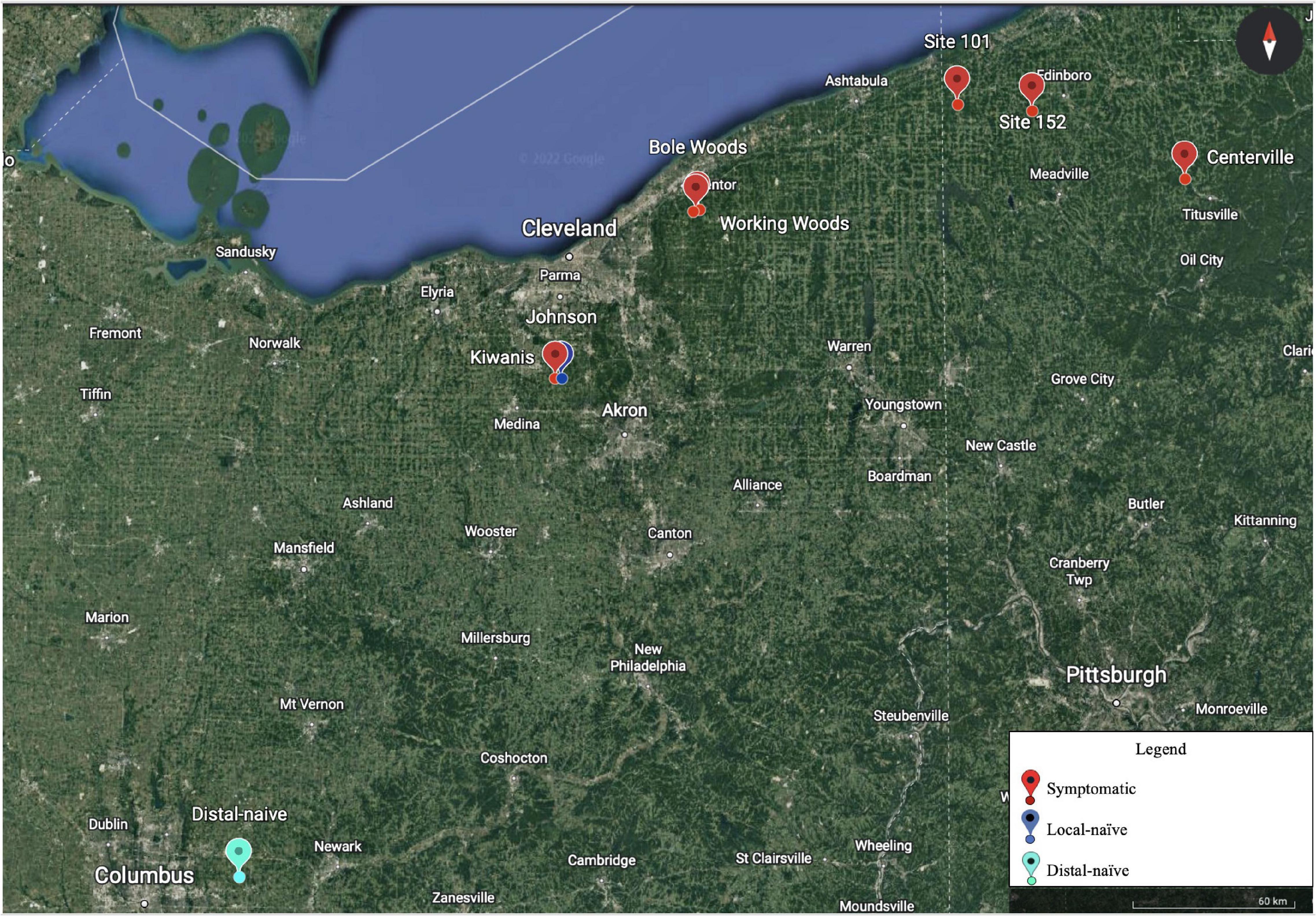
Figure 1. Eight sampling plots were chosen for the near-infrared (NIR) spectral collection over the various time points in Ohio and Pennsylvania. The symptom type of each plot is indicated by the color in the legend (Google Earth 9. 156. 0. 0, 2022).

In May and July, spectral measurements were taken from five asymptomatic leaves on each of ten symptomatic trees (hereafter referred to as pre-symptomatic) in the five symptomatic plots, except for the Centerville site which included 17 trees (N = 168 and 281 for May and July, respectively), and from ten healthy leaves on each of 20 trees from the distal-naïve plot (N = 180 and 200 for May and July, respectively). In September, spectral measurements were taken from 10 asymptomatic leaves on each of 10 symptomatic trees in the Kiwanis plot (N = 71) and 10 healthy leaves on each of 10 trees from the local-naïve plot (N = 100). Spectra were collected from easily accessible leaves in the lower canopy. However, due to varying levels of BLD severity in symptomatic plots and the inaccessibility of leaves of each symptom type in the lower canopy, it was not always possible to collect the same number of leaves from each tree, which is why the number of spectral samples vary between the months. In addition, spectra from sites 101 and Working Woods could not be collected in May due to unfavorable weather conditions. The spectra were collected at the top right portion of the adaxial side of each leaf to maximize consistency across samples. The NIR spectra were collected using a handheld NeoSpectra Scanner (Si-Ware Systems, Menlo Park, CA, United States) with a two-second collection time and a resolution of 16 nm as measured at 1,550 nm. The NeoSpectra Scanner has its own optical, mechanical, and electrical components combined on one chip that allows the quality and intensity of incident light to be consistent across readings (Si-Ware, 2021). The spectral range of the instrument is 1,350–2,500 nm. A two-second background measurement was collected between each tree using a white reference surface provided with the Scanner. The spectra were collected, visualized, and exported using the NeoSpectra Scan Android application (Si-Ware Systems).

Spectrum pre-processing

Following modified methods from Conrad et al. (2020), the raw NIR spectra were imported into R version 4.0.3 (R Core Team, 2021), and outliers were detected and trimmed using packages “fda.usc” and “fda” (Febrero-Bande and Oviedo la Fuenta, 2012; Ramsay et al., 2020). Outliers were identified based on the assumption that the depth of the spectral curve and the sample’s outlyingness are inversely related (Febrero-Bande and Oviedo la Fuenta, 2012Febrero-Bande and Oviedo de la Fuenta 2012). Additional outliers were identified and removed based on abnormal NIR reflectance intensities determined using boxplots. From the 348 spectra collected in May, seven spectra were identified as outliers and removed using the depth-based approach and two were removed based on abnormalities at the 1,843 and 1,692 nm wavelengths (N = 339). For the July dataset consisting of 481 spectra, 58 spectra were removed due to machine malfunction at site 101. In addition, 28 spectra were identified as outliers and removed using the depth-based approach and two outliers were removed based on abnormalities at the 1,349 and 1,877 nm wavelengths (N = 393). In September, four spectra were removed using the depth-based approach only (N = 167).

Machine learning

Spectra were transformed to the second derivative using the package “mdatools” with the following parameters: width of filter window = 15, porder = 2, and dorder = 2 (Conrad et al., 2020; Kucheryavskiy, 2020). All datasets were randomly split into training (70% of data) and testing (30%) sets using the package “caret” (Kuhn, 2020) (Supplementary Table 1). Supervised classification models were developed using SVM, with scaling, using the package “e1071” (Meyer et al., 2021) and random forest using packages “randomForest” (Liaw and Wiener, 2002) and “VSURF” (Genuer et al., 2019). Optimal parameters for both models were determined using a 10-fold cross validation (Supplementary Table 2). Model performance was evaluated using package “MLmetrics” (Yan, 2016) and assessed based on the total accuracy from the training and testing set and the 10-fold cross validated accuracy on the training set. In addition, receiver operating characteristic (ROC) curves were generated to evaluate the testing set accuracy using the package “ROCR” for SVM models and “pROC” for random forest models (Sing et al., 2005; Robin et al., 2011).

To avoid overfitting the models, three variable reduction methods were performed. The first method called “VarImp,” uses the “caret” package (Kuhn, 2020) to calculate the importance of each spectral band in influencing the response (symptom type), and the second uses the random forest model to identify spectral bands that are associated with the response using the package “VSURF” (Genuer et al., 2019). The “VSURF” method identifies two sets of variables: interpretation and prediction (Genuer et al., 2019). While both sets of variables are related to the response, the prediction variables are more refined than the interpretation variables as they eliminate any redundancy from the interpretation variables. Finally, a method using spectral resampling that reduces the total number of bands included in the analysis was performed using the package “prospectr” (Stevens and Ramirez-Lopez, 2020). We selected a bin size of five to reduce multicollinearity without adversely impacting the model performance by decreasing the number of bands too severely (Conrad et al., 2020). This reduced the total number of bands used in the analysis from 74 to 15.

Finally, we used sparse partial least squares discriminant analysis (sPLS-DA) to confirm the identities of important spectral bands across analyses using the package “mixOmics” (Rohart et al., 2017). A repeated five-fold cross-validation with 50 repeats of the training set was used to identify the optimal number of components and variables for each component that discriminated between the symptom types. The accuracy of the model was evaluated based on the proportion of samples correctly classified in the testing set and the balanced error rate (BER) of the predictions of the testing set.

To further confirm the differences in spectral profiles between symptom types in the September dataset, we also conducted an analysis of variance (ANOVA) using the package “stats” (R Core Team, 2021) on the average transformed reflectance values of the key bands shared by all of the variable reduction models that select for important wavelengths, including VarImp, VSURF, and sPLS-DA.

DNA extraction and qPCR

After the NIR spectra collection in September, the ten local-naïve and pre-symptomatic leaves as well as an additional five banded, five crinkled, and five pre-symptomatic leaves from trees in the other symptomatic plots and ten leaves from trees in the distal-naïve plot were collected and temporarily stored on ice before being placed in a –80°C freezer for long-term storage. The leaves were bulked per tree based on symptom type and ground in liquid nitrogen. In total, there were 20 distal-naïve, 46 pre-symptomatic, 10 local-naïve, 32 banded, and 16 crinkled samples used for DNA extractions. Total DNA was extracted from 50 mg of ground tissue using Qiagen’s DNeasy Plant Pro Kit (Qiagen, Germantown, MD, United States). The quality of the extracted DNA was confirmed using a NanoDrop UV 1000 Visible spectrophotometer (Thermo Fisher Scientific, Waltham, MA, United States).

To quantify LCM in each of the sample types, each sample was run in triplicate as technical replicates, along with a non-template control and a positive control using LCM DNA, for TaqMan^® determined using the equation qPCR using primers and probe that target a 122-bp region of the mitochondrial cytochrome c oxidase I specific to LCM (Marra et al., in preparation).

qPCR sensitivity and quantification

Standards were prepared in triplicate to generate two types of calibration curves for LCM DNA and nematode count. A 10-fold dilution series of extracted LCM DNA was used to generate a standard curve to quantify the amount of nematode DNA in each sample. Since we did not know the amount of DNA in a single LCM nematode, we quantified the number of nematodes per gram of leaf tissue by creating standards of 1, 10, and 100 nematodes. Nematodes were extracted from symptomatic leaves collected from West Rock Ridge State Park in New Haven, CT in September 2021. The nematodes were counted using a dissecting microscope and aliquoted into 100 μl of a potassium buffer saline (PBS) solution (pH of 7.0). The aliquots were added to 20 mg of ground naïve leaf tissue along with 500 μl of the DNeasy Plant Pro kit’s CD1 solution and 20 μl of Proteinase K and incubated at 56°C overnight. DNA extractions proceeded following the DNeasy Plant Pro Kit protocol.

To determine the amount of LCM DNA and individual nematodes present in each technical replicate, the C_q values from each standard were plotted against the corresponding log₁₀ value of the starting DNA concentration or nematode count to create two separate standard curves (Supplementary Figures 1, 2). The derived amount of DNA or number of nematodes was then averaged for the three technical replicates, with the number of nematodes rounded to the nearest whole number, and the standard error was reported. The equation of the standard curve was used to determine the coefficient of determination (R²), and the amplification efficiency was determined using the equation E = 10^(–1/m)–1 × 100%, where m is the slope of the standard curve. Because we did not use a standard DNA serial dilution for nematode counts and amplification efficiencies generally decrease when using individual organisms as standards (Zemb et al., 2020), especially when using an extreme variable such as a count of one nematode (Chowdhury and Yan, 2021), we expected the efficiency of the qPCR using the nematode count standards to be lower than the qPCR using the LCM DNA series. A Welch’s ANOVA was used to determine if there were significant differences in DNA concentration or nematode numbers at p = 0.05 based on symptom type. A Welch’s ANOVA was used due to the heteroscedasticity of the data (Moder, 2010). If a significant difference was found, a Tukey’s honestly significant difference (HSD) test was used to calculate pairwise comparisons at the 95% confidence level.

Results

May and July NIR spectral analysis

The average raw and second derivative transformed spectra for each symptom type from the May and July datasets can be found in Figure 2. The overall shape of the second derivative plots from both time periods are similar, but the intensities for the symptom types differ, specifically between the wavelengths 1,353–1,451 nm, 1,697–1,854 nm, and 1,854–2,043 nm. The trimmed spectral range for both the May and July analyses included 74 bands ranging from 1,349 to 2,581 nm. The number of bands was reduced further when using spectral resampling (15 bands) and variable selection techniques. For both the May and July datasets, VarImp reduced the number of bands to 20 and VSURF reduced the bands to 13 for the interpretation step variables while the prediction step reduced the number of bands to eight in May and nine in July (Supplementary Table 3). The sPLS-DA analysis also selected variables of importance for the optimal number of components for the May (five components) and July (three components) data (Supplementary Table 4). Only one band (2346) was shared in all analyses between the two time periods.

FIGURE 2

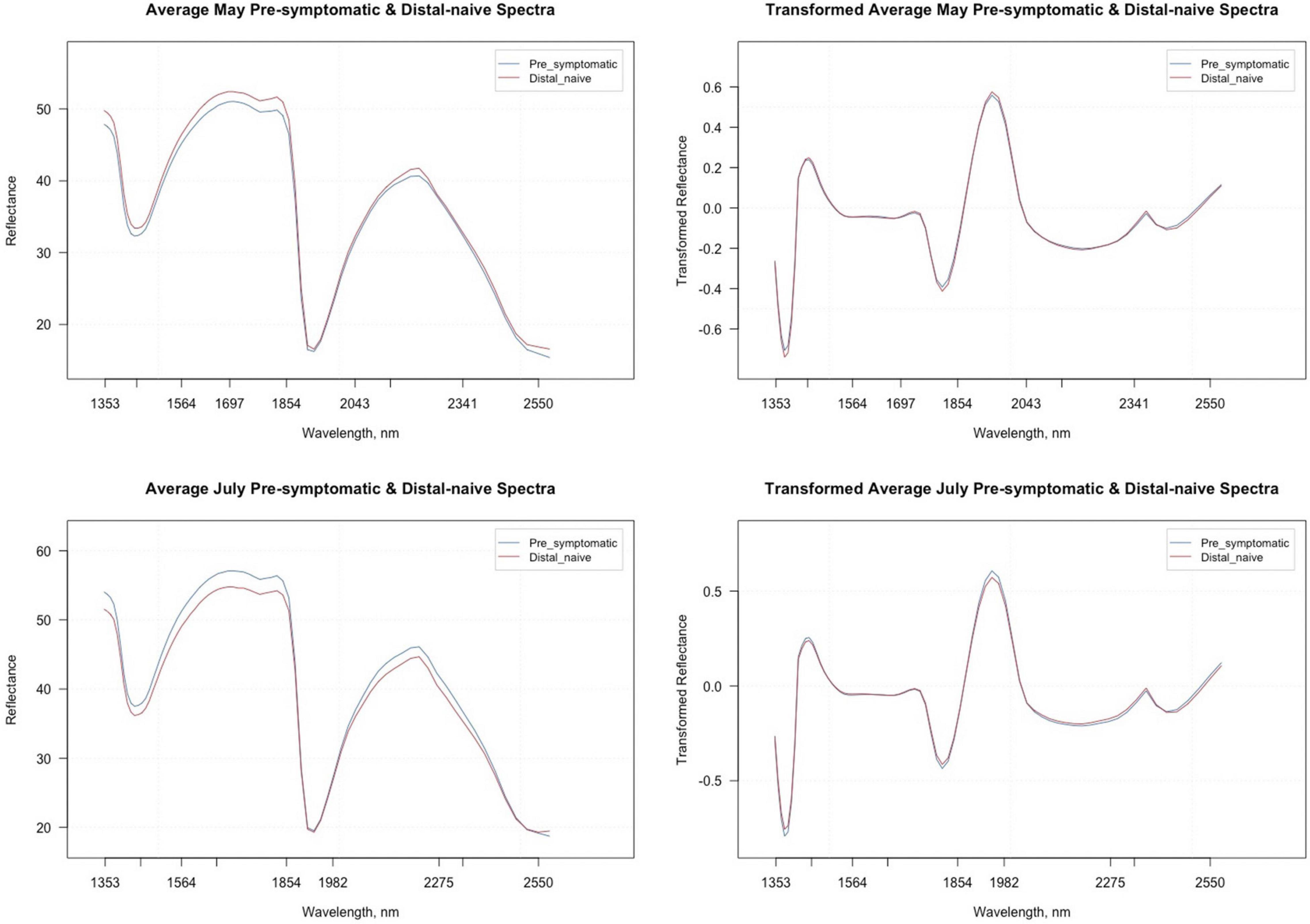
Figure 2. Average raw and second derivative transformed spectral signatures of pre-symptomatic (excluding the Kiwanis site) and distal-naïve samples in May and July.

All analyses using SVM had a 10-fold cross-validated accuracy greater than 90% and a testing accuracy greater than 85% for both the May and July datasets (Table 1). The SVM using all spectral bands had the greatest testing accuracy for both time points (91% for May; 100% for July) and the greatest 10-fold cross-validated accuracy for the July data (100%), while spectral resampling had the greatest 10-fold cross validated accuracy for the May data (97.5%). ROC curves assessing the testing accuracy of all SVM models for both time points can be seen in Figure 3. The accuracy of the models was lower when using random forest, but all analyses still had a 10-fold cross-validated accuracy and testing accuracy greater than 80% for both time points (Table 2). When using random forest, the model using all spectral bands had the greatest testing accuracy for July (94.9%) and both this model and the VSURF interpretation model had the greatest testing accuracy for the May data (90%). The VSURF interpretation step had the greatest 10-fold cross validated accuracy for the May data (94%) while the VSURF prediction step had the greatest for July (94.9%). ROC curves assessing the accuracy of the testing sets for all random forest models for both time points can be seen in Figure 4. The sPLS-DA showed similar total accuracies for both the May (86.1%) and the July (95.7%) testing sets (Table 3).

TABLE 1

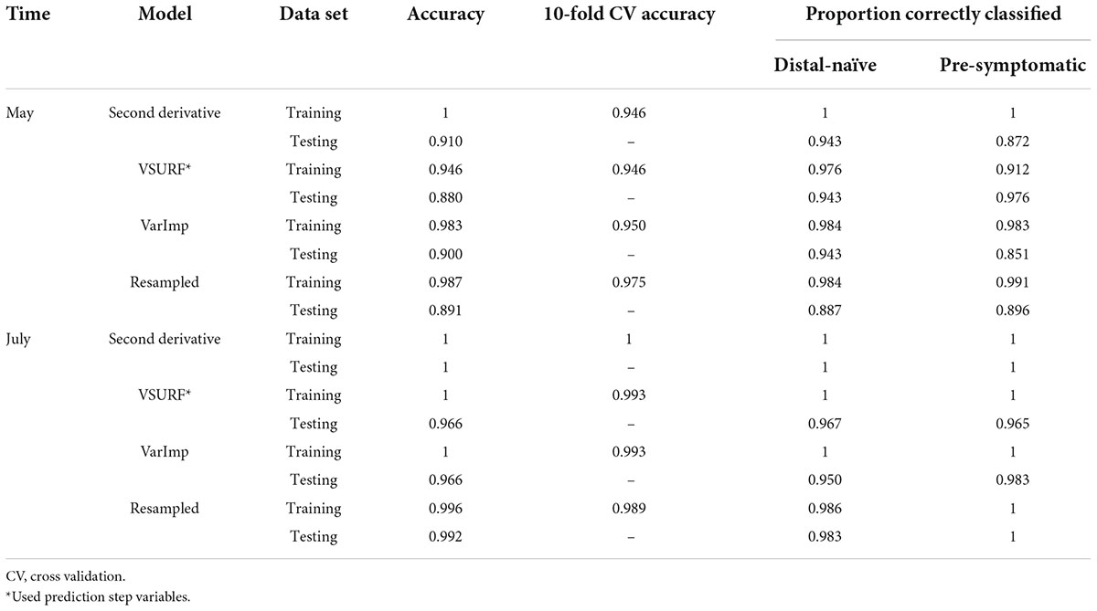
Table 1. Accuracies of the four distinct support vector machine (SVM) models used to classify leaf near-infrared (NIR) spectra based on tree symptom type for the May and July datasets.

FIGURE 3

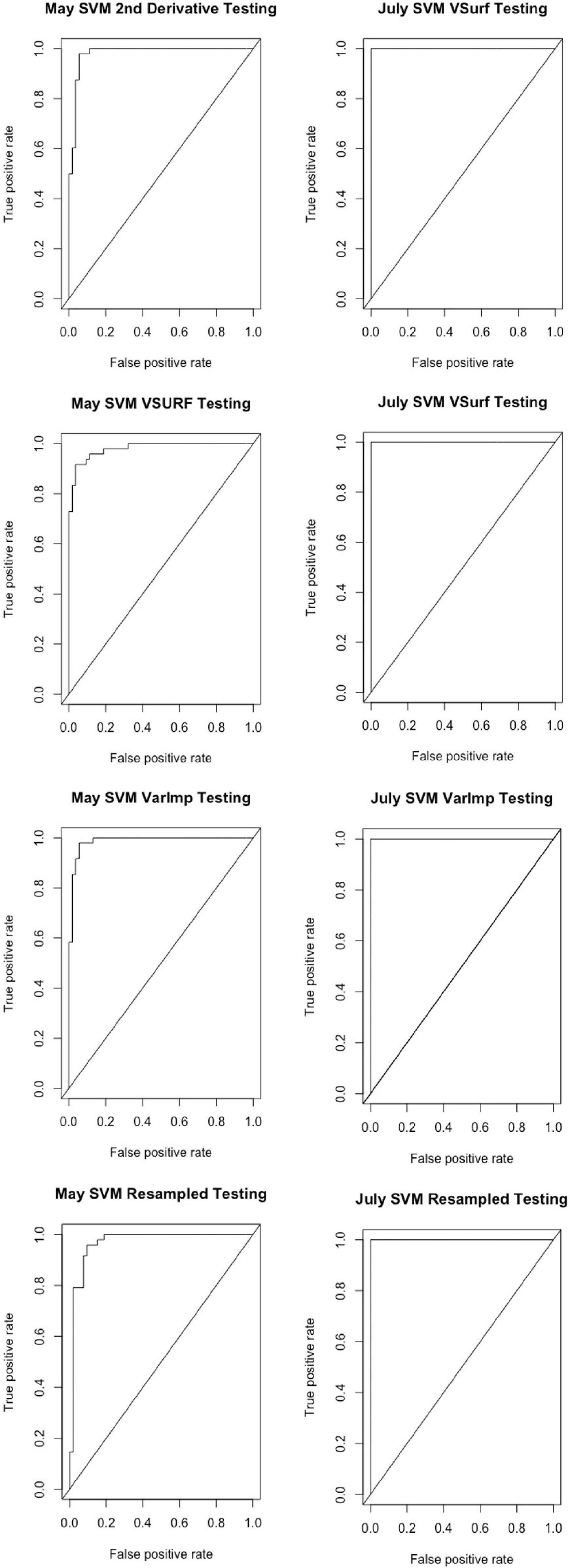
Figure 3. Receiver operating characteristic (ROC) curves derived from the testing of the support vector machine (SVM) models, showing the classification accuracy of spectra from pre-symptomatic (excluding the Kiwanis site) and distal-naïve samples for both the May (left) and July (right) datasets. The diagonal line represents perfect chance predictions.

TABLE 2

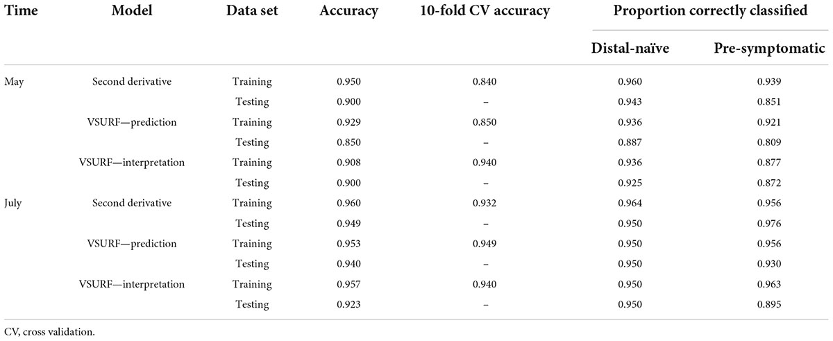
Table 2. Accuracies of the three distinct random forest models used to classify leaf near-infrared (NIR) spectra based on tree symptom type for the May and July datasets.

FIGURE 4

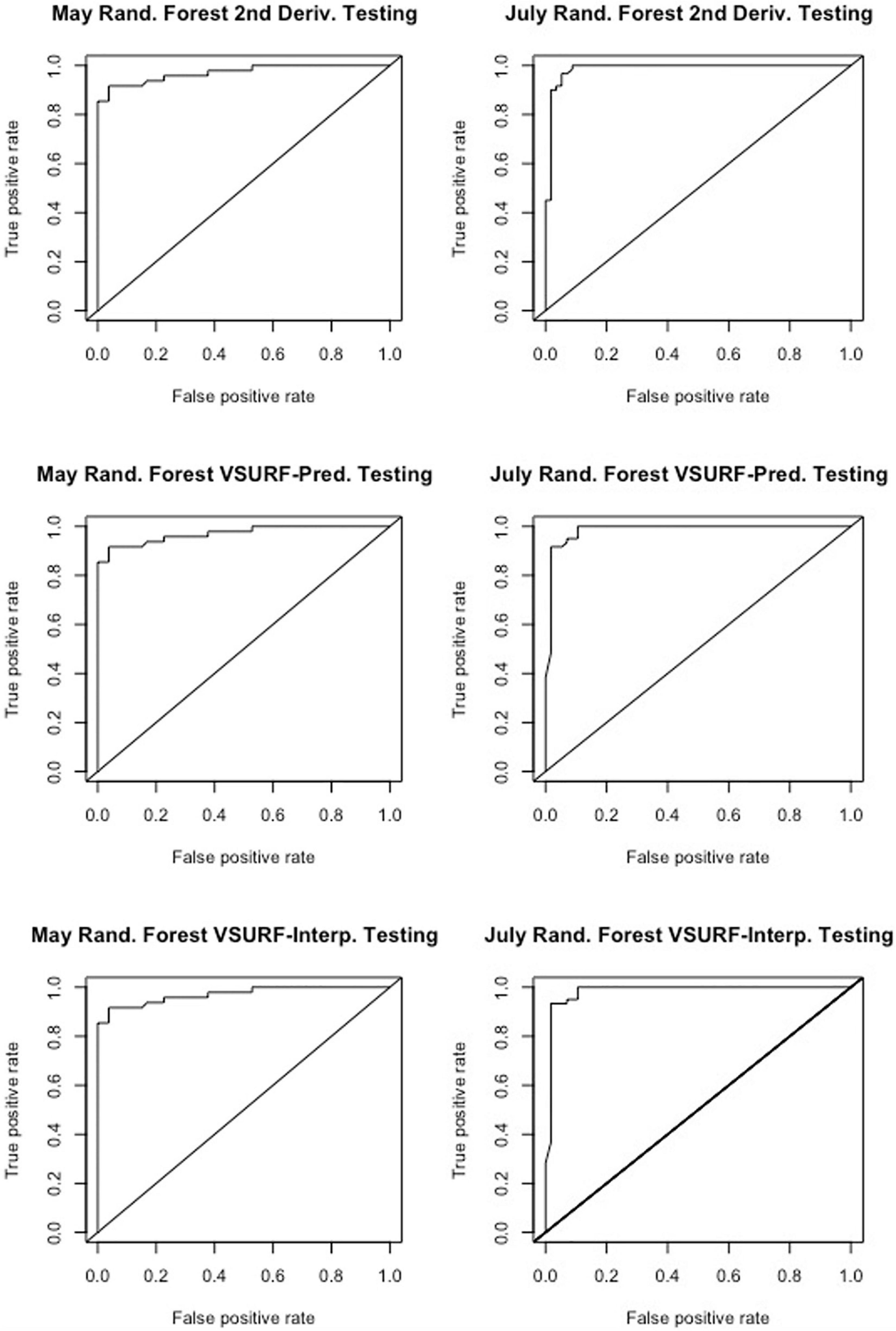
Figure 4. Receiver operating characteristic (ROC) curves derived from the testing of the random forest models, showing the classification accuracy of spectra from pre-symptomatic samples (excluding the Kiwanis site) and distal-naïve samples for the both the May (left) and July (right) datasets. The diagonal line represents perfect chance predictions.

TABLE 3

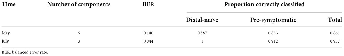
Table 3. Accuracies of the sparse partial least squares discriminant analysis (sPLS-DA) used to classify leaf near-infrared (NIR) spectra based on tree symptom type for the May and July datasets.

The average raw and second derivative transformed spectra for each plot location can be seen in Supplementary Figure 3. When using SVM with all spectral bands, the total 10-fold cross-validated and testing accuracies were greater than 90% for both the May and July datasets (Table 4). This strongly suggests that plot location does influence the leaf spectra.

TABLE 4

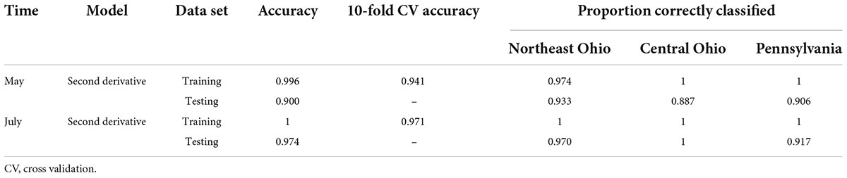
Table 4. Accuracies of the support vector machine (SVM) model used to classify leaf near-infrared (NIR) spectra based on site location for the May and July datasets.

September NIR spectral analysis

Figure 5 shows the average raw and second derivative transformed spectra for the local-naïve and pre-symptomatic leaves from the September collection time, which removes location as a confounding factor. When looking at the second derivative spectra, the spectral intensities between the two symptom types do not appear to differ from one another. The variable selection techniques reduced the total number of bands from 74 to 20 for VarImp, 25 for the VSURF interpretation step, and eight for the VSURF prediction step (Supplementary Table 3). The sPLS-DA analysis selected important variables for four components and shared many of the same bands as the variable selection techniques (Supplementary Table 4). Five bands were shared among all analyses (2,220, 2,400, 2,346, 1,750, and 1,424), and the ANOVA showed that the average transformed reflectance intensities of these bands were significantly different based on symptom type (p « 0.001).

FIGURE 5

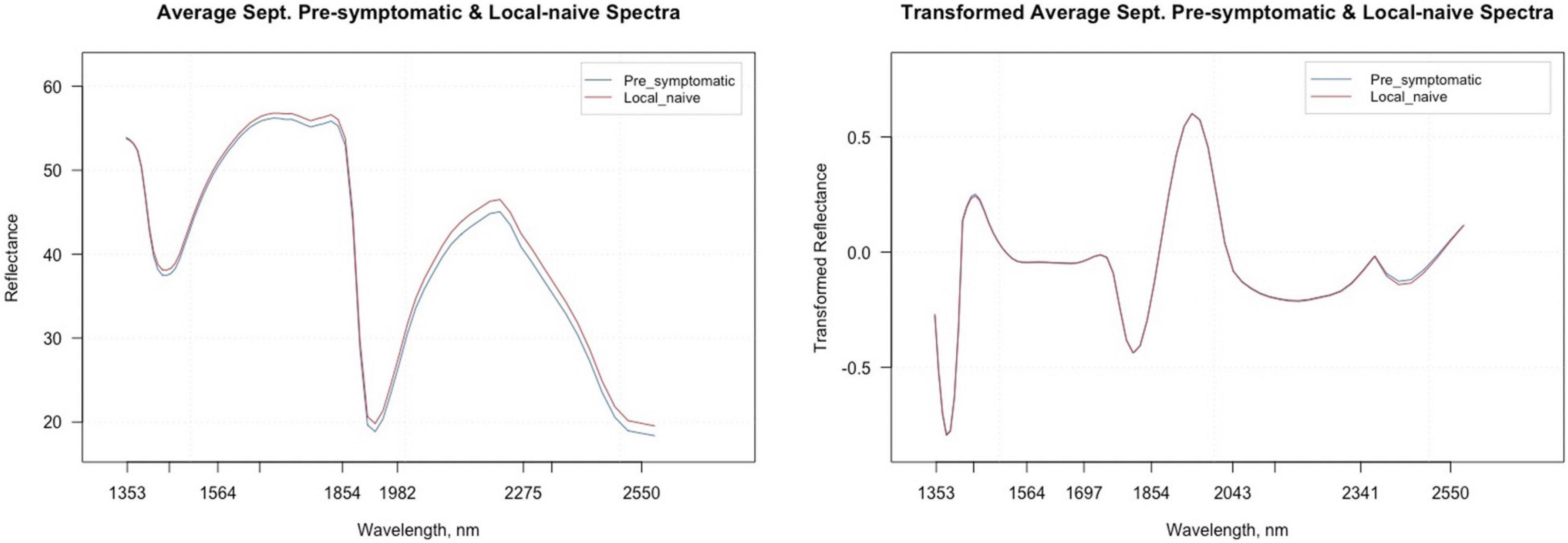
Figure 5. Average raw and second derivative transformed spectral signatures of pre-symptomatic samples from only the Kiwanis site and local-naïve samples in September.

All SVM analyses had a testing accuracy greater than 70% and a 10-fold cross-validated accuracy greater than 75% (Table 5). The model using all spectral bands had the highest testing accuracy (95.9%) while the resampled dataset had the highest 10-fold cross validated accuracy (96.6%). The random forest testing and 10-fold cross-validated accuracies were slightly higher than the SVM analyses (Table 6). The VSURF prediction step and interpretation steps had the greatest testing (79.6%) and 10-fold cross-validated (87.8%) accuracies for the random forest models, respectively. ROC curves evaluating the accuracy of the testing sets for all SVM and random forest models can be seen in Figure 6. For both SVM and random forest, the models were better at accurately classifying the spectra from local-naïve trees. Finally, the sPLS-DA analysis showed similar results as it was able to accurately classify 93.9% of the spectra in the testing set (Table 7).

TABLE 5

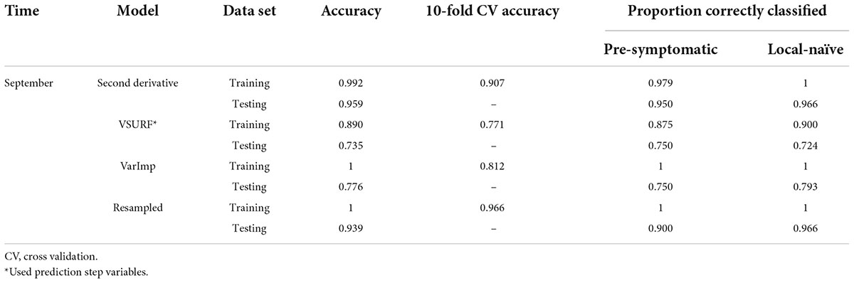
Table 5. Accuracies of the four distinct support vector machine (SVM) models used to classify leaf near-infrared (NIR) spectra based on tree symptom type for the September dataset.

TABLE 6

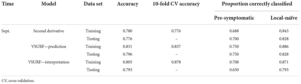
Table 6. Accuracies of the three distinct random forest models used to classify leaf near-infrared (NIR) spectra based on tree symptom type for the September dataset.

FIGURE 6

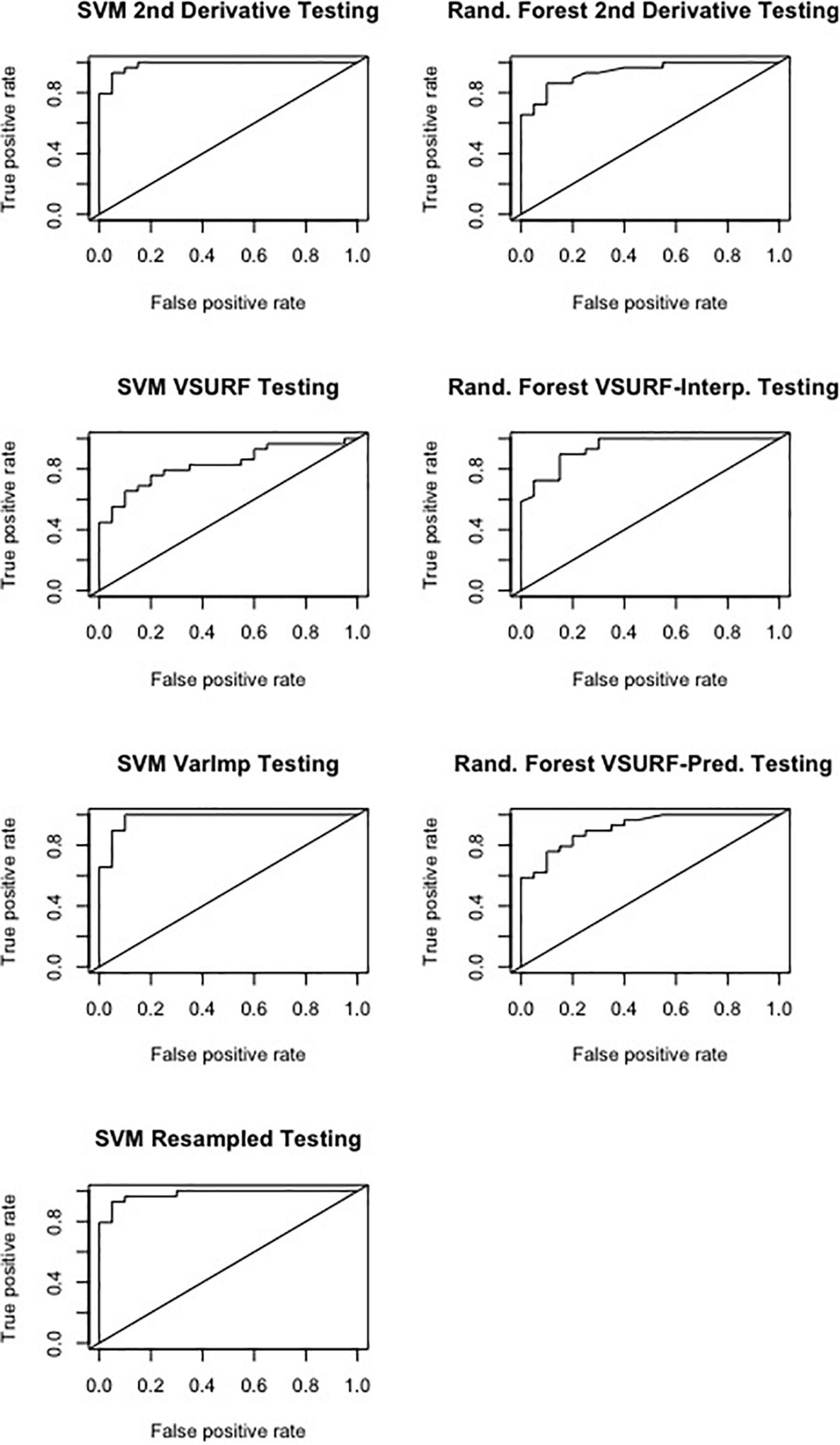
Figure 6. Receiver operating characteristic (ROC) curves derived from the testing of the support vector machine (SVM) (left) and random forest (right), showing the classification accuracy of spectra from pre-symptomatic samples from only the Kiwanis site and local-naïve samples for the September dataset. The diagonal line represents perfect chance predictions.

TABLE 7

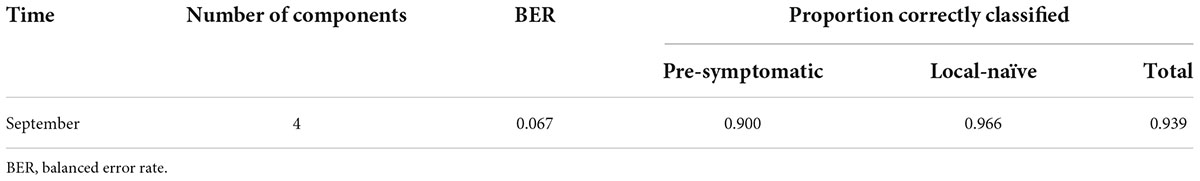
Table 7. Accuracy of the sparse partial least squares discriminant analysis (sPLS-DA) used to classify near-infrared (NIR) spectra based on tree symptom type for the September dataset.

qPCR results

The efficiency of the qPCR analysis when using the 10-fold dilution series of LCM DNA was 93.4% and the standard curve resulted in an R² value of 0.997 and a slope of –3.492 (Supplementary Figure 1). The qPCR detected LCM DNA in all 16 crinkled samples, 30 of the 32 banded samples, and 42 of the 46 pre-symptomatic samples while LCM DNA was only detected in four of the 20 distal-naïve samples and two of the ten local-naïve samples. The crinkled samples had the greatest average DNA concentration (39.2 ± 9.8 ng/μl; average C_q = 14.25 ± 0.34) while the distal-naïve samples had the lowest (1.66e-06 ± 9.79e-07 ng/μl; average C_q = 36.65 ± 0.64) (Figure 7A). There was a significant difference in the LCM DNA concentration based on symptom type (p « 0.001), but only the crinkled DNA concentration differed significantly from the other sample types based on the post-hoc test. There was also a slightly significant difference in DNA concentration (p = 0.0646) between the local-naïve samples (4.37e-06 ± 3.02e-06 ng/μl; average C_q = 35.32 ± 0.34) and the pre-symptomatic samples (0.008 ± 0.003 ng/ml; average C_q = 26.99 ± 0.59) from the Kiwanis site (Figure 8A).

FIGURE 7

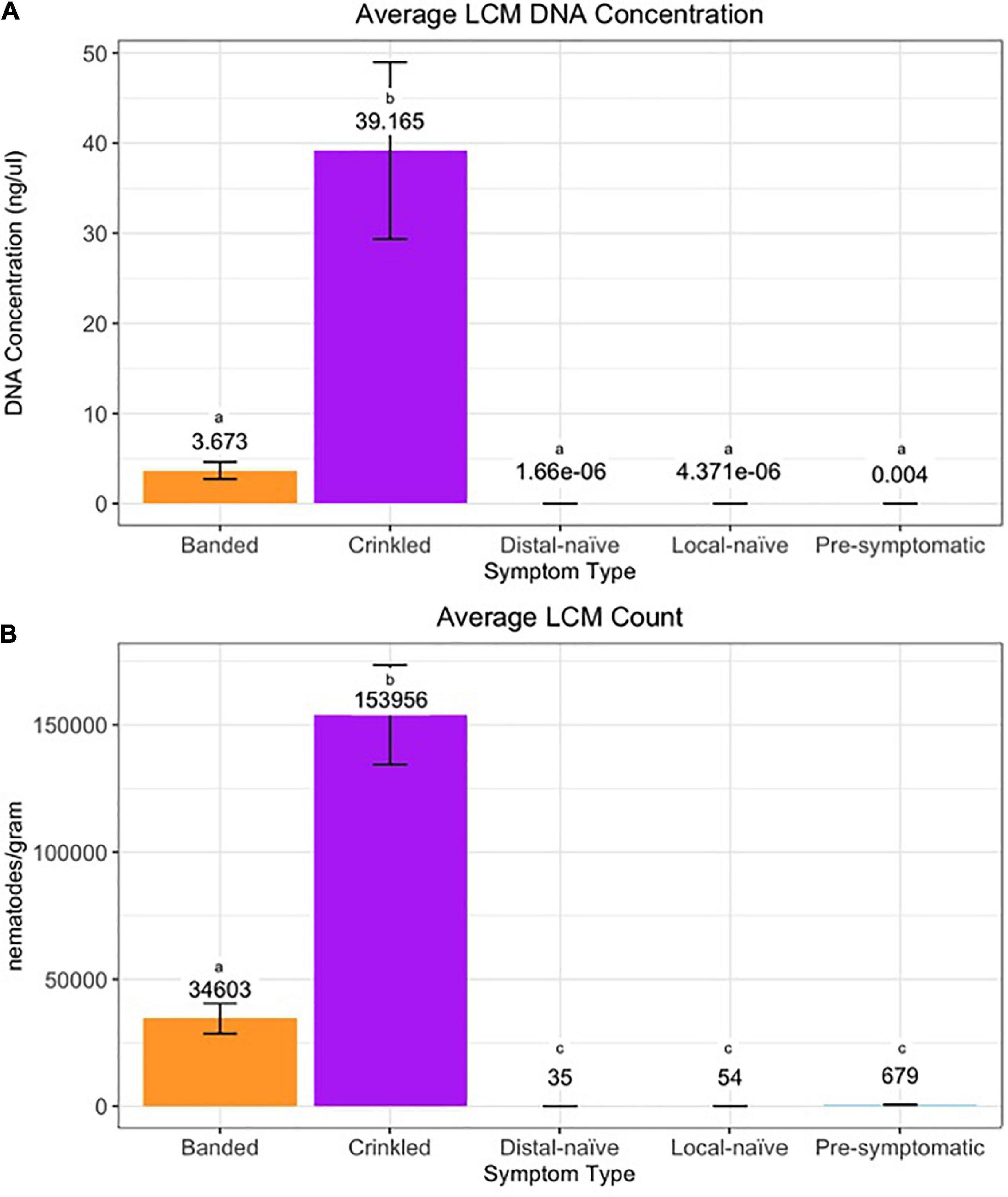
Figure 7. (A) DNA concentration and (B) count per symptom type of Litylenchus crenatae mccannii (LCM). Error bars represent the standard error. Actual DNA concentration and nematode counts are listed above the bars and significant differences (p < 0.05) between symptom types are represented by different letters.

FIGURE 8

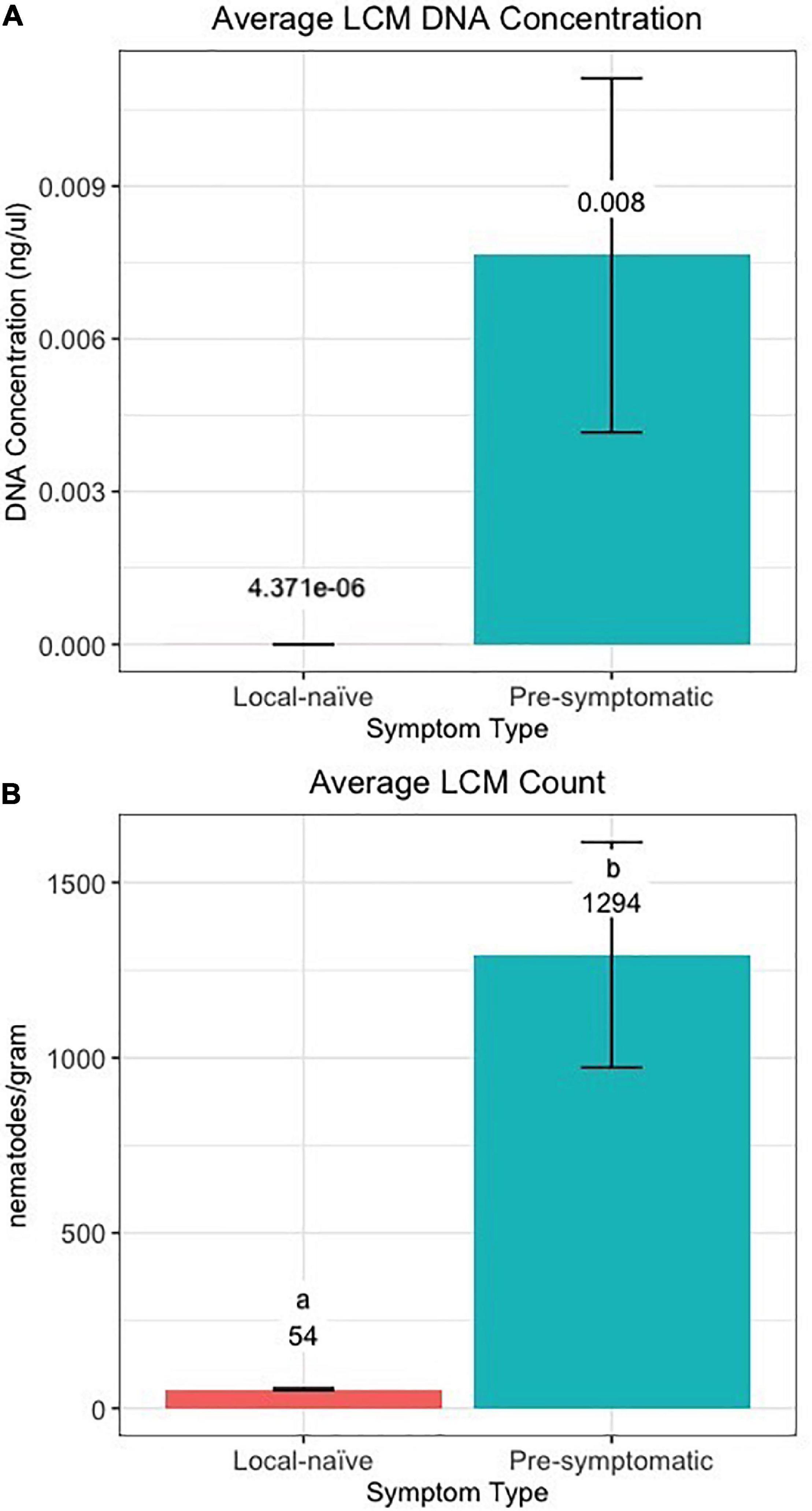
Figure 8. (A) DNA concentration and (B) count of Litylenchus crenatae mccannii (LCM) in local-naïve samples and pre-symptomatic samples from only the Kiwanis site. Actual concentration and nematode counts are listed above the bars and significant differences (p < 0.05) between symptom types are represented by different letters.

When we used individual nematodes and not a serial dilution of DNA, the qPCR efficiency was only 45%, and the standard curve resulted in an R² value of 0.877 and a slope of –6.240 (Supplementary Figure 2). Similar to the results from the qPCR based on pure DNA, crinkled samples had the greatest average number of nematodes (153,956 ± 19,552.9) per gram of leaf tissue while the distal-naïve (35 ± 2.9) and local-naïve (54 ± 3.2) samples had the least (Figure 7B). These differences were highly significant between sample types according to the ANOVA (p « 0.001), as shown in Figure 8B. The average nematode count was also significantly different between local-naïve samples and pre-symptomatic samples from the Kiwanis location (p = 0.002) (Figure 8B).

Discussion

The results of this study indicate that NIR spectroscopy coupled with ML can discriminate asymptomatic leaves of healthy trees and asymptomatic leaves of symptomatic trees, therefore showing promise as an early in-field BLD detection pipeline, which was the intended objective of this study. However, while spectra from pre-symptomatic leaves and distal-naïve leaves were discriminated with high accuracy in both the May and July datasets, the NIR spectra were also differentiated based on plot location, with equal or higher accuracies for location than symptom type. Thus, we could not conclude that the spectral differences in this dataset are due to the presence of LCM alone. This is not surprising, as climate and other environmental variables, as well as host genetics and the phytobiome, have all been shown to influence leaf chemical composition, and these factors are all affected by geographic location (Holdenrieder et al., 2004; Top et al., 2017; Liu et al., 2020). In a recent study focusing specifically on American beech trees, it was discovered that the microbiome, especially the mycobiome, of American beech leaves is significantly differentiated by geographic location (Ewing et al., 2021). Based on these results, we can conclude that tree location must be considered when using NIR spectral analysis for early disease detection.

However, the September analysis eliminated location, and presumably population genetics, as factors given that the Kiwanis and Johnson sites are adjacent. Again, the technology successfully discriminated between leaves from pre-symptomatic trees and leaves from local-naïve trees based on their NIR spectral profiles. In all SVM and random forest models, the testing accuracies ranged from 73.5 to 95.9%. These accuracies are comparable to other studies that have used NIR spectroscopy for early plant disease detection (Rumpf et al., 2010; Arens et al., 2016). For example, in the study that used NIR spectroscopy and machine learning algorithms to predict rice sheath blight before symptoms were expressed, the testing accuracies were between 60.4 and 88.6% (Conrad et al., 2020). These results suggest that chemical changes are occurring in asymptomatic American beech leaves following pathogen infection and indicate that NIR spectroscopy, combined with machine learning, has strong potential for use as a tool for pre-symptomatic disease detection.

Although no visual differences were noticeable between the average second derivative transformed spectra profiles for pre-symptomatic and local-naïve samples, there were five bands (2,220, 2,400, 2,346, 1,750, and 1,424 nm) that were shared across all variable selection models in the September dataset, and the average transformed reflectance of each band was significantly different based on symptom type as indicated by the ANOVA. The band at 2,346 was also shared among all analyses from the May and July datasets. The bands located at 2,400, 2,346, and 1,750 nm are closely related to bands previously reported to be associated with plant cellulose (Curran, 1989). In addition, the 2,220 nm band is near the band (2,180) associated with protein and nitrogen in plants according to Curran (1989). Therefore, it is possible that changes in the cell wall and/or increases in cellulose-degrading enzymes and nitrogen following attack from the BLD pathogen(s) could be responsible for the changes in spectral composition of the pre-symptomatic samples (Schultz et al., 2013; Malinovsky et al., 2014).

The 1,424 nm band is most closely related to band 1,420 nm, which is associated with lignin (Curran, 1989). Lignin is one of the most important specialized metabolites of plants and is an important barrier that protects against pests and pathogens (Liu et al., 2018). Lignin has also been associated with an increase in plant resistance as the cell wall accumulates large amounts of lignin following a pathogen infection, and it has been shown to reduce pathogen proliferation and movement (Liu et al., 2018). In one example, Mandal et al. (2013) confirmed that lignin concentrations were higher in tomato varieties that are resistant to the pathogen Ralstonia solanacearum compared to susceptible cultivars. More specific examples associated with resistance in trees include studies showing that enhanced lignin deposition is related to systemic induced resistance in Austrian pines (Pinus nigra) afflicted with the fungal pathogen Diplodia sapinea (ex Sphaeropsis sapinea) (Bonello and Blodgett, 2003; Bonello et al., 2006). Furthermore, when testing the antifungal properties of several phenolic compounds in Austrian pine, lignin showed the greatest antifungal activity and was also necessary for fungistatic inhibition against D. sapinea (Sherwood and Bonello, 2013).

Given this information, it is possible that lignin levels are higher in the local-naïve beech samples and serving as a barrier to LCM/pathogen infection, which could be responsible for the changes in the spectral profile compared to pre-symptomatic samples. While the exact BLD disease cycle has not been clearly defined, studies show that LCM overwinters in American beech buds as well as attached and detached leaves; live nematodes are found in leaves throughout the growing season with the greatest numbers found in late summer/early fall (Carta et al., 2020; Reed et al., 2020). Since BLD symptoms are present at bud break and do not progress throughout the season (Fearer et al., 2022), this suggests that LCM causes symptoms prior to bud break, which Carta et al. (2020) confirmed in their study, and LCM migration into the leaf occurs sometime before September (Reed et al., 2020). Therefore, it is possible that higher lignin levels in local-naïve leaves are preventing LCM/pathogen infection prior to bud break. However, a further detailed chemical analysis of beech bud and leaf tissues would have to be performed and the LCM life cycle as well as the BLD disease cycle would have to be better defined to validate these hypotheses.

Another hypothesis is that LCM load influences the leaf’s phytochemistry and may be the determining factor for early BLD detection using NIR spectroscopy. While LCM DNA was putatively detected in all symptom types using qPCR, the C_q values reported for the distal-naïve and local-naïve samples were greater than 35; these values are indistinguishable from zero and may be due to random late-cycle probe hydrolysis (Ruiz-Villalba et al., 2021). In addition, the low qPCR efficiency of the nematode count standard curve could lead to C_q-dependent biases when interpolating nematode counts from the standard curve (Ruiz-Villalba et al., 2021). Therefore, it is more likely that all distal-naïve and local-naïve samples are LCM-free. In any case, symptomatic samples had significantly more LCM DNA, and correspondingly higher nematode loads, than all asymptomatic samples (i.e., pre-symptomatic, distal-naïve, and local-naïve), and pre-symptomatic samples harbored more LCM than both distal-naïve and local-naïve samples, confirming our hypothesis. Most strikingly, pre-symptomatic samples from the Kiwanis site had significantly more LCM DNA, and correspondingly higher numbers of nematodes, than local-naïve samples from the Johnson site. This suggests that the higher numbers of nematodes in pre-symptomatic samples are responsible for the measured changes in the spectral profiles, and therefore, LCM count should be taken into consideration when building NIR/ML-based models to identify pre-symptomatic trees.

Conclusion

NIR/ML-based modeling seems to be a promising approach for early BLD detection. This study determined that the spectral profiles of visually identical American beech leaves can be discriminated based on the infection state of the tree and suggests that LCM population sizes influence these spectral differences. Based on these results, this approach appears to be a viable, early in-field disease detection tool for BLD. However, geographical distance between sampling locations must be taken into consideration prior to sampling to account for potential differences in host genetics and phenology. Specifically, models should be standardized for each general location and time of year. The system should be further verified on the ground by testing its predictive power using molecular confirmation of nematode load by way of the LCM-specific qPCR assay described in this study or similarly accurate methods. Only if the predictive power of the tool is confirmed on an operational basis can it be recommended for use by forest health managers.

Finally, further characterization of the leaf chemical composition of asymptomatic leaves from pre-symptomatic trees could help uncover the biological basis for potential resistance. Development of resistant germplasm by breeding and/or preserving resistant trees is critical to prevent the functional eradication of American beech in North American forests. Non-native pathogens will inevitably become permanent fixtures in our native ecosystems, and genetic resistance provides an invaluable tool for managing the diseases associated with these invaders (Conrad and Bonello, 2016; Showalter et al., 2018; Bonello et al., 2020).

Data availability statement

The raw data supporting the conclusions of this article will be made available by the authors, without undue reservation.

Author contributions

CF, PB, AC, JS, and CV contributed to the conception and design of the study. CF and CG conducted NIR spectra collection and performed the statistical analyses. CF performed qPCR and wrote first draft of the manuscript. All authors contributed to manuscript revision, read, and approved the submitted version.

Funding

Funding for this project was provided through USDA Forest Service cooperative agreement 19-DG-11132544-028.

Conflict of interest

The authors declare that the research was conducted in the absence of any commercial or financial relationships that could be construed as a potential conflict of interest.

Publisher’s note

All claims expressed in this article are solely those of the authors and do not necessarily represent those of their affiliated organizations, or those of the publisher, the editors and the reviewers. Any product that may be evaluated in this article, or claim that may be made by its manufacturer, is not guaranteed or endorsed by the publisher.

Acknowledgments

We thank Shane Allan and Elizabeth White for their assistance with the spectral collection and nematode counting. We also thank Constance Hausman and Daniel Volk at Cleveland Metroparks and David Burke at Holden Arboretum for providing plot locations. The use of trade names is for the information and convenience of the reader and does not imply official endorsement or approval by the USDA or the Forest Service of any product to the exclusion of others that may be suitable.

Supplementary material

The Supplementary Material for this article can be found online at: https://www.frontiersin.org/articles/10.3389/ffgc.2022.934545/full#supplementary-material

References

Arens, N., Backhaus, A., Döll, S., Fischer, S., Seiffert, U., and Mock, H.-P. (2016). Non-invasive presymptomatic detection of Cercospora beticola infection and identification of early metabolic responses in sugar beet. Front. Plant Sci. 7:01377. doi: 10.3389/fpls.2016.01377

PubMed Abstract | CrossRef Full Text | Google Scholar

Baret, F., Houlès, V., and Guérif, M. (2007). Quantification of plant stress using remote sensing observations and crop models: the case of nitrogen management. J. Exp. Bot. 58, 869–880. doi: 10.1093/jxb/erl231

PubMed Abstract | CrossRef Full Text | Google Scholar

Bois, E., and Lieutier, F. (1997). Phenolic response of Scots pine clones to inoculation with Leptographium wingfieldii, a fungus associated with Tomicus piniperda. Plant Physiol. Biochem. 35, 819–825.

Google Scholar

Bonello, P., and Blodgett, J. T. (2003). Pinus nigra-Sphaeropsis sapinea as a model pathosystem to investigate local and systemic effects of fungal infection of pines. Physiol. Mol. Plant Pathol. 63, 249–261. doi: 10.1016/j.pmpp.2004.02.002

CrossRef Full Text | Google Scholar

Bonello, P., Campbell, F. T., Cipollini, D., Conrad, A. O., Farinas, C., Gandhi, K. J. K., et al. (2020). Invasive tree pests devastate ecosystems—a proposed new response framework. Front. For. Glob. Chang. 3:2. doi: 10.3389/ffgc.2020.00002

CrossRef Full Text | Google Scholar

Bonello, P., Gordon, T. R., Herms, D. A., Wood, D. L., and Erbilgin, N. (2006). Nature and ecological implications of pathogen-induced systemic resistance in conifers: a novel hypothesis. Physiol. Mol. Plant Pathol. 68, 95–104. doi: 10.1016/j.pmpp.2006.12.002

CrossRef Full Text | Google Scholar

Carta, L. K., Handoo, Z. A., Li, S., Kantor, M. R., Bauchan, G., McCann, D., et al. (2020). Beech leaf disease symptoms caused by newly recognized nematode subspecies Litylenchus crenatae mccannii (Anguinata) described from Fagus grandifolia in North America. For. Pathol. 50:e12580. doi: 10.1111/efp.12580

CrossRef Full Text | Google Scholar

Chowdhury, I. A., and Yan, G. (2021). Development of real-time and conventional PCR assays for identifying a newly named species of root-lesion nematode (Pratylenchus dakotaensis) on soybean. Int. J. Mol. Sci. 22:5872. doi: 10.3390/ijms22115872

PubMed Abstract | CrossRef Full Text | Google Scholar

Conrad, A. O., and Bonello, P. (2016). Application of infrared and Raman spectroscopy for the identification of disease resistant trees. Front. Plant Sci. 6:1152. doi: 10.3389/fpls.2015.01152

PubMed Abstract | CrossRef Full Text | Google Scholar

Conrad, A. O., Li, W., Lee, D.-Y., Wang, G.-L., Rodrigues-Saona, L., and Bonello, P. (2020). Machine learning-based presymptomatic detection of rice sheath blight using spectral profiles. Plant Phenom. 2020:8954085. doi: 10.34133/2020/8954085

PubMed Abstract | CrossRef Full Text | Google Scholar

Curran, P. J. (1989). Remote sensing of foliar chemistry. Remote Sens. Environ. 30, 271–278. doi: 10.1016/0034-4257(89)90069-90062

CrossRef Full Text | Google Scholar

Ewing, C. J., Hausman, C. E., Pogacnik, J., Slot, J., and Bonello, P. (2019). Beech leaf disease: an emerging forest epidemic. For. Pathol. 49:e12488. doi: 10.1111/efp.12488

CrossRef Full Text | Google Scholar

Ewing, C. J., Slot, J., Benítez Ponce, M.-S., Rosa, C., Malacrinò, A., Bennett, A., et al. (2021). The foliar microbiome suggests fungal and bacterial agents may be involved in the beech leaf disease pathosystem. Phytobiomes J. 5, 335–349. doi: 10.1094/PBIOMES-12-20-0088-R

CrossRef Full Text | Google Scholar

Fang, Y., and Ramasamy, R. P. (2015). Current and prospective methods for plant disease detection. Biosensors 5, 537–561. doi: 10.3390/bios5030537

PubMed Abstract | CrossRef Full Text | Google Scholar

Fearer, C. J., Volk, D., Hausman, C. E., and Bonello, P. (2022). Monitoring foliar symptom expression in beech leaf disease through time. For. Pathol. 52:e12725. doi: 10.1111/efp.12725

CrossRef Full Text | Google Scholar

Febrero-Bande, M., and de la Fuenta, M. (2012). Statistical computing in functional data analysis: the R package fda.usc. J. Stat. Softw. 51, 1–28. doi: 10.18637/jss.v051.i04

CrossRef Full Text | Google Scholar

Fiehn, O. (2001). Combining genomics, metabolome analysis, and biochemical modelling to understand metabolic networks. Comp. Funct. Genomics 2, 155–168. doi: 10.1002/cfg.82

PubMed Abstract | CrossRef Full Text | Google Scholar

Genuer, R., Poggi, J.-M., and Tuleau-Malot, C. (2019). VSURF: Variable Selection Using Random Forests. R Package Version 1.1.0. Available online at: https://CRAN.R-project.org/package=VSURF.

Google Scholar

Gervasi, S. S., Civitello, D. J., Kilvitis, H. J., and Martin, L. B. (2015). The context of host competence: a role for plasticity in host-parasite dynamics. Trends Parasitol. 31, 419–425. doi: 10.1016/j.pt.2015.05.002

PubMed Abstract | CrossRef Full Text | Google Scholar

Gold, K. M., Townsend, P. A., Larson, E. R., Herrmann, I., and Gevens, A. J. (2020). Contact reflectance spectroscopy for rapid, accurate, and nondestructive Phytophthora infestans clonal lineage discrimination. Phytopathology 110, 851–862. doi: 10.1094/PHYTO-08-19-0294-R

PubMed Abstract | CrossRef Full Text | Google Scholar

Google Earth 9. 156. 0. 0 (2022). Beech Leaf Disease. 40°58’29”N, 81°11’41”W, Eye alt. 247 m. Borders and labels; landmarks; Water Layers. Washington, DC: Landsat/Copernicus, NOAA.

Google Scholar

Griffin, G. J. (2000). Blight control and restoration of the American chestnut. J. For. 98, 22–27. doi: 10.1093/jof/98.2.22

CrossRef Full Text | Google Scholar

Holdenrieder, O., Pautasso, M., Weisberg, P. J., and Lonsdale, D. (2004). Tree diseases and landscape processes: the challenge of landscape pathology. Trends Ecol. Evol. 19, 446–452. doi: 10.1016/j.tree.2004.06.003

PubMed Abstract | CrossRef Full Text | Google Scholar

Kralik, P., and Ricchi, M. (2017). A basic guide to real time PCR in microbial diagnostics: definitions, parameters, and everything. Front. Microbiol. 8:108. doi: 10.3389/fmicb.2017.00108

PubMed Abstract | CrossRef Full Text | Google Scholar

Kucheryavskiy, S. (2020). mdatools - R package for chemometrics. Chemom. Intell. Lab. Syst. 198:103937. doi: 10.1016/j.chemolab.2020.103937

CrossRef Full Text | Google Scholar

Kuhn, M. (2020). Caret: Classification and Regression Training. R package version 6.0-91. Available online at: https://CRAN.R-project.org/package=caret.

Google Scholar

Lee, J. A., Halbert, S. E., Dawson, W. O., and Singer, B. H. (2015). Asymptomatic spread of huanglongbing and implications for disease control. PNAS 112, 7605–7610. doi: 10.1073/pnas.1508253112

PubMed Abstract | CrossRef Full Text | Google Scholar

Liaw, A., and Wiener, M. (2002). Classification and regression by random Forest. R. News 2, 18–22.

Google Scholar

Liu, H., Brettell, L. E., and Singh, B. (2020). Linking the phyllosphere microbiome to plant health. Trends Plant Sci. 25, 841–844. doi: 10.1016/j.tplants.2020.06.003

PubMed Abstract | CrossRef Full Text | Google Scholar

Liu, Q., Luo, L., and Zheng, L. (2018). Lignins: biosynthesis and biological functions in plants. Int. J. Mol. Sci. 19:335. doi: 10.3390/ijms19020335

PubMed Abstract | CrossRef Full Text | Google Scholar

Malinovsky, F. G., Fangel, J. U., and Willats, W. G. T. (2014). The role of the cell wall in plant immunity. Front. Plant Sci. 5:178. doi: 10.3389/fpls.2014.00178

PubMed Abstract | CrossRef Full Text | Google Scholar

Mandal, S., Kar, I., Mukherjee, A. K., and Acharya, P. (2013). Elicitor-induced defense responses in Solanum lycopersicum against Ralstonia solanacearum. Sci. World J. 2013:561056. doi: 10.1155/2013/561056

PubMed Abstract | CrossRef Full Text | Google Scholar

Martin, J. A., Solla, A., Venturas, M., Collada, C., Dominguez, J., Miranda, E., et al. (2015). Seven Ulmus minor clones tolerant to Ophiostoma novo-ulmi registered as forest reproductive material in Spain. iForest - Biogeosci. For. 8, 172–180. doi: 10.3832/ifor1224-008

PubMed Abstract | CrossRef Full Text | Google Scholar

Martinelli, F., Scalenghe, R., Davino, S., Panno, S., Scuderi, G., Ruisi, P., et al. (2015). Advanced methods of plant disease detection. a review. Agron. Sustain. Dev. 35, 1–25. doi: 10.1007/s13593-014-0246-241

CrossRef Full Text | Google Scholar

Mascaro, J., Asner, G. P., Knapp, D. E., Kennedy-Bowdoin, T., Martin, R. E., Anderson, C., et al. (2014). A tale of two “forests”: random forest machine learning aids tropical forest carbon mapping. PLoS One 9:e85993. doi: 10.1371/journal.pone.0085993

PubMed Abstract | CrossRef Full Text | Google Scholar

Meyer, D., Dimitriadou, E., Hornik, K., Weingessel, A., and Leisch, F. (2021). e1071: Misc Functions of the Department of Statistics, Probability Theory Group (formerly: E1071). Vienna: TU Wien.

Google Scholar

Moder, K. (2010). Alternatives to F-test in one way ANOVA in case of heterogeneity of variances (a simulation study). Psychol. Test Assess. Model. 52, 343–353.

Google Scholar

R Core Team (2021). R: A Language and Environment for Statistical Computing. Vienna: R Core Team.

Google Scholar

Ramsay, J. O., Graves, S., and Hooker, G. (2020). fda: Functional Data Analysis. R Package Version 5.5.1. Available online at: https://cran.r-project.org/package=fda.

Google Scholar

Reed, S., Greifenhagen, S., Yu, Q., Hoke, A. J., Burke, D. J., Carta, L. K., et al. (2020). Foliar nematode, Litylenchus crenatae spp. mccannii, population dynamics in leaves and buds of beech leaf disase-affected trees in Canada and the US. For. Pathol. 50:e12599. doi: 10.1111/efp.12599

CrossRef Full Text | Google Scholar

Robin, X., Turck, N., Alexandre, H., Tilberti, N., Lisacek, F., Sanchez, J.-C., et al. (2011). pROC: an open-source package for R and S+ to analyze and compare ROC curves. BMC Bioinform. 12:77. doi: 10.1186/1471-2105-12-77

PubMed Abstract | CrossRef Full Text | Google Scholar

Rohart, F., Gautier, B., Singh, A., and Le Cao, K.-A. (2017). mixOmics: an R package for ’omics feature selection and multiple data integration. PLoS Comput. Biol. 13:e1005752. doi: 10.1371/journal.pcbi.1005752

PubMed Abstract | CrossRef Full Text | Google Scholar

Ruiz-Villalba, A., Ruijter, J. M., and van den Hoff, M. J. B. (2021). Use and misuse of Cq in qPCR data analysis and reporting. Life (Basel, Switzerland) 11:496. doi: 10.3390/life11060496

PubMed Abstract | CrossRef Full Text | Google Scholar

Rumpf, T., Mahlein, A.-K., Steiner, U., Oerke, E.-C., Dehne, H.-W., and Plümer, L. (2010). Early detection and classification of plant diseases with support vector machines based on hyperspectral reflectance. Comput. Electron. Agric. 74, 91–99. doi: 10.1016/j.compag.2010.06.009

CrossRef Full Text | Google Scholar

Schaad, N. W., and Frederick, R. D. (2002). Real-time PCR and its application for rapid plant disease diagnostics. Can. J. Plant Pathol. 24, 250–258. doi: 10.1080/07060660209507006

CrossRef Full Text | Google Scholar

Schratz, P., Muenchow, J., Iturritxa, E., Cortés, J., Bischl, B., and Brenning, A. (2021). Monitoring forest health using hyperspectral imagery: does feature selection improve the performance of machine learning techniques? Remote Sens. 13:23. doi: 10.3390/rs13234832

CrossRef Full Text | Google Scholar

Schultz, J., Appel, H., Ferrieri, A., and Arnold, T. (2013). Flexible resource allocation during plant defense responses. Front. Plant Sci. 4:324. doi: 10.3389/fpls.2013.00324

PubMed Abstract | CrossRef Full Text | Google Scholar

Sherwood, P., and Bonello, P. (2013). Austrian pine phenolics are likely contributors to systemic induced resistance against Diplodia pinea. Tree Physiol. 33, 845–854. doi: 10.1093/treephys/tpt063

PubMed Abstract | CrossRef Full Text | Google Scholar

Showalter, D. N., Villari, C., Herms, D. A., and Bonello, P. (2018). Drought stress increased survival and development of emerald ash borer larvae on coevolved Manchurian ash and implicates phloem-based traits in resistance. Agric. For. Entomol. 20, 170–179. doi: 10.1111/afe.12240

CrossRef Full Text | Google Scholar

Si-Ware (2021). NeoSpectra Scanner. Available online at: https://www.si-ware.com/products-and-software/neospectra-scanner.

Google Scholar

Sing, T., Sander, O., Beerenwinkel, N., and Lengauer, T. (2005). ROCR: visualizing classifier performance in R. Bioinformatics 21:7881. doi: 10.1093/bioinformatics/bti623

PubMed Abstract | CrossRef Full Text | Google Scholar

Singh, A., Ganapathysubramanian, B., Singh, A. K., and Sarkar, S. (2016). Machine learning for high-throughput stress phenotyping in plants. Trends Plant Sci. 21, 110–124. doi: 10.1016/j.tplants.2015.10.015

PubMed Abstract | CrossRef Full Text | Google Scholar

Stevens, A., and Ramirez-Lopez, L. (2020). An Introduction to the Prospectr Package. R Package Viggnette R Package Version 0.2.4.

Google Scholar

Top, S. M., Preston, C. M., Dukes, J. S., and Tharayil, N. (2017). Climate influences the content and chemical composition of foliar tannins in green and senesced tissues of Quercus rubra. Front. Plant Sci. 8:423. doi: 10.3389/fpls.2017.00423

PubMed Abstract | CrossRef Full Text | Google Scholar

Viiri, H., Annila, E., Kitunen, V., and Niemelä, P. (2001). Induced responses in stilbenes and terpenes in fertilized Norway spruce after inoculation with blue-stain fungus, Ceratocystis polonica. Trees 15, 112–122.

Google Scholar

Witzell, J., and Martín, J. A. (2008). Phenolic metabolites in the resistance of northern forest trees to pathogens — past experiences and future prospects. Can. J. For. Res. 38, 2711–2727. doi: 10.1139/X08-112

CrossRef Full Text | Google Scholar

Yan, Y. (2016). MLmetrics: Machine Learning Evaluation Metrics. R Package Version 1.1.1. Available online at: https://CRAN.R-project.org/package=MLmetrics.

Google Scholar

Zemb, O., Achard, C. S., Hamelin, J., De Almeida, M., Gabinaud, B., Cauquil, L., et al. (2020). Absolute quantitation of microbes using 16S rRNA gene metabarcoding: a rapid normalization of relative abundances by quantitative PCR targeting a 16S rRNA gene spike-in standard. Microbiologyopen 9:e977. doi: 10.1002/mbo3.977

PubMed Abstract | CrossRef Full Text | Google Scholar