Joint impacts of future climate conditions and invasive species on black ash forested wetlands

Introduction

Shifts in temperature and shifts in the timing, frequency, and quantity of precipitation associated with climate change are already impacting global wetland ecology and these impacts are expected to intensify into the future (Burkett and Kusler, 2000; Moomaw et al., 2018). In general, the Great Lakes region of North America is expected to see declining summer precipitation while total annual precipitation stays stable or increases (Hayhoe et al., 2010; Byun and Hamlet, 2018). These projected changes result in increased precipitation in the spring and winter months. Winter precipitation will also experience a phase change, seeing a reduction in the proportion of precipitation as snow, increased occurrence of rain-on-snow melt events in the winter and spring, and earlier snowmelt timing (Notaro et al., 2015). Our study area in the western Upper Peninsula of Michigan, United States is projected to receive increased winter precipitation and a slight decrease to slight increase in summer precipitation dependent on emissions scenarios and model (Byun and Hamlet, 2018). Based upon numerous downscaling scenarios across multiple general circulation models (GCMs), local conditions are expected to vary within a region and our study area is projected to have wetter summer conditions relative to much of the Great Lakes region (Byun and Hamlet, 2018). The shift in precipitation timing and magnitude, the reduction of total snowfall, and an earlier onset of snowmelt will reshape the annual hydrologic budget. These changes will alter wetland hydroperiods, with water availability increasing in the winter and spring and decreasing in the summer and early fall. Throughout the Great Lakes region, including our study area (Byun and Hamlet, 2018), summer temperatures are expected to increase 2–8°C (Hayhoe et al., 2010; Byun and Hamlet, 2018). The resulting increased evaporative demand is expected to outpace any projected increase in summer precipitation, leading to more frequent drought conditions and increased water stress on ecosystems (Byun and Hamlet, 2018).

Black ash (Fraxinus nigra Marsh.) is an important hardwood component of many forested wetlands in the northern United States and southern Canada. In addition to climate-change induced impacts, black ash wetlands face the loss of the major canopy species due to an invasive insect, Emerald ash borer (Agrilus planipennis Fairmaire, EAB). Emerald ash borer was first found in the United States in southeastern Michigan in 2002 (Haack et al., 2002). It is known to infest and cause high mortality in all ash native to North America (Herms and McCullough, 2014). As of this writing, EAB is present in 35 US states and five Canadian provinces and has invaded the western Upper Peninsula of Michigan in 2020 (APHIS, 2021). High mortality, the importance of ash in regional forested wetlands, and cultural significance of black ash in regional indigenous communities have led to research on the impacts of their loss and strategies to mitigate those impacts. Iverson et al. (2016) evaluated potential replacement species for black ash in the context of habitat availability, species migration, and replacement species susceptibility to climate change impact, providing a useful resource for climate-informed species replacements for black ash. However, black ash grows in a range of geomorphic settings, and local site conditions can have a strong influence on hydrology, forest structure, and wetland plant community (Kolka et al., 2018). Considering both Iverson et al. (2016) and Kolka et al. (2018), we can identify four necessary components to evaluate mitigation efforts in black ash wetlands: (1) climate-informed species selection, (2) species tolerance of local site conditions, (3) site conditions following EAB infestation, and (4) site conditions in a future climate.

Previous and ongoing work in Michigan and Minnesota has assessed mitigation for components 1–3 that inform the combined impact of climate change and EAB on black ash wetlands. Researchers in Michigan (Bolton et al., 2018), Minnesota (Looney et al., 2015), and Wisconsin (Bolton et al., 2018) planted seedlings to evaluate potential canopy species at the wetland rather than landscape level. The plantings in Looney et al. (2015) and Bolton et al. (2018) took place under simulated EAB infestation, where the seedlings were subjected to adverse conditions due to the hydrologic impact of the loss of black ash (Slesak et al., 2014; Van Grinsven et al., 2017), as well as the increased competition from herbaceous growth under increased light conditions (Looney et al., 2016, 2017; Davis et al., 2017). This present study aims to integrate the results of the mitigation assessments presented in these previous studies to enhance our understanding of components 3 and 4, and to specifically assess selection of climate-informed species.

Of particular importance for this study is that the above mitigation assessment research in black ash wetlands incorporated (1) evaluation of targeted planted species at the northern edge of their current range, evaluated impacts (2) under present-day site conditions and (3) under simulated-EAB site conditions. It was not feasible for these field studies to address the interaction of EAB and climate change on site conditions. Just as we have seen EAB impacts cascade through black ash ecosystems affecting hydrology, plant communities, and nutrient cycling, we can expect the future climate-driven changes to hydrology to result in similar cascades. Focusing on the future hydrologic characteristics of these wetlands will inform the impacts to other functions, given hydrology is the critical control on wetland ecosystems (Brinson, 1993). To understand future hydrologic conditions, we have developed wetland water level models and evaluated potential changes in water levels under future climate scenarios and potential changes in black ash stands as a result of EAB.

Wetland water levels in black ash wetlands in northern Minnesota and northern Michigan were significantly higher following girdling and cutting treatments where wetter site conditions in conjunction with delayed timing and decreased rates of drawdown during the growing season demonstrate the hydrologic conditions that will likely exist following the EAB-induced loss of ash (Slesak et al., 2014; Van Grinsven et al., 2017). Co-dominant canopy species in black-ash dominant wetlands, including red maple (Acer rubrum L.) and yellow birch (Betula alleghaniensis Britt.) were shown to have significantly lower sap flux when compared to black ash across the entire gradient of observed water level conditions (Shannon et al., 2018), and ultimately these lower rates contributed to the significantly lower site transpiration estimates detected in girdled and ash-cut treatments when compared to black ash control treatments in northern Michigan wetlands (Van Grinsven et al., 2017). Previous studies have also demonstrated high-interannual variation in seasonal wetland water level drawdown and rebound in black ash wetlands (Van Grinsven et al., 2017). Estimating the behavior of a highly variable system with a small number of weather sequences could lead to biased or high-variance results, making it difficult to draw proper conclusions about the combined impacts of climate change and EAB. Simulation studies of future conditions should be performed on a large number of weather sequences that represent the variability of observable weather under a given climate scenario. Stochastic weather generators (SWGs) provide a tool for generating synthetic time series of weather that simulate conditions under an observed or projected climate (Wilks and Wilby, 1999).

We have performed simulation experiments combining observed wetland hydrology and synthetic weather sequences to quantify the interactions of EAB and future climate scenarios. We developed wetland hydrology models for black ash forested conditions (current ash-dominated forested wetlands), non-forested conditions (herbaceous and shrub/scrub wetlands), and alternate-forested conditions (forested wetlands comprised of current co-dominant species). Specifically, we used overstory and understory plant community composition observed in black ash wetlands before and after simulated-EAB site conditions (Looney et al., 2015; Davis et al., 2017) to develop the wetland hydrology models for black ash forested, alternate-forested, and non-forested wetland condition classes, respectively. We evaluated each class of wetland model under two potential future climate scenarios for the end of the twenty-first century (2070–2099). The two future scenarios are defined by a moderate representative concentration pathway (RCP 4.5) projected using a less sensitive GCM, and a business-as-usual representative concentration pathway (RCP 8.5) projected using a more sensitive GCM (van Vuuren et al., 2011). GCMs were considered as more or less sensitive based on the magnitude of projected change under a given RCP scenario (Byun and Hamlet, 2018). The two-scenario “bookend” approach provides a range of potential future conditions as opposed to an ensemble approach which masks some of the uncertainty in potential future conditions by reporting the mean of possible scenarios (Swanston et al., 2016). As a result, each class of wetland model, including black ash forested, alternate-forested, and non-forested, were evaluated for each ‘bookend’ model, respectively, resulting in a total of six model evaluations.

We expect that the interaction of hydrologic impacts of EAB and climate change will result in a tempering of the two individual impacts in this region. While simulation of post-EAB conditions have led to increased water levels and reduced drawdown rates in the growing season, future climate conditions in the region will result in reduced water availability during that same period. These two opposing drivers should result in some moderation to both impacts.

Materials and methods

Study sites and data

Wetland water levels measured from 2012 to 2020 at eight black ash-dominated wetlands in the western Upper Peninsula of Michigan, United States were used to develop and evaluate our wetland hydrologic models (Figure 1 and Table 1). The wetlands range in size from 0.29 to 1.54 ha and 30–80% of the basal area consists of black ash with histosol soils over an unconsolidated mineral layer located at an average depth of 118.8 cm (Davis et al., 2017; Van Grinsven et al., 2017). The region has average minimum and maximum annual temperatures of −11.3 and 18.2°C and an average annual precipitation of 101 cm for the climate period of 1980–2009 at the Bergland Dam (46°35′13′′N, 89°32′51′′W) meteorological station (Arguez et al., 2012). Wetland water levels were continuously monitored in 2′′ inner-diameter driven wells from 2012 to 2020 and logged every 15 min using Solinst Levellogger Junior pressure transducers (Solinst, Ontario, CA, United States), with more details available in Van Grinsven et al. (2017). Barometric compensation was performed using data from Solinst Levellogger Junior pressure transducers deployed at a subset of study wetlands. Compensated water levels were corrected for temperature differentials as in Shannon et al. (2022). Following an initial control period of two growing seasons, all of the wetlands used in this study were treated to simulate the impacts of an EAB infestation. All ash trees greater than 1” in diameter were girdled in three sites and all ash trees greater than 1” in diameter were hand-felled and left on site in the remaining five sites (Table 1).

FIGURE 1

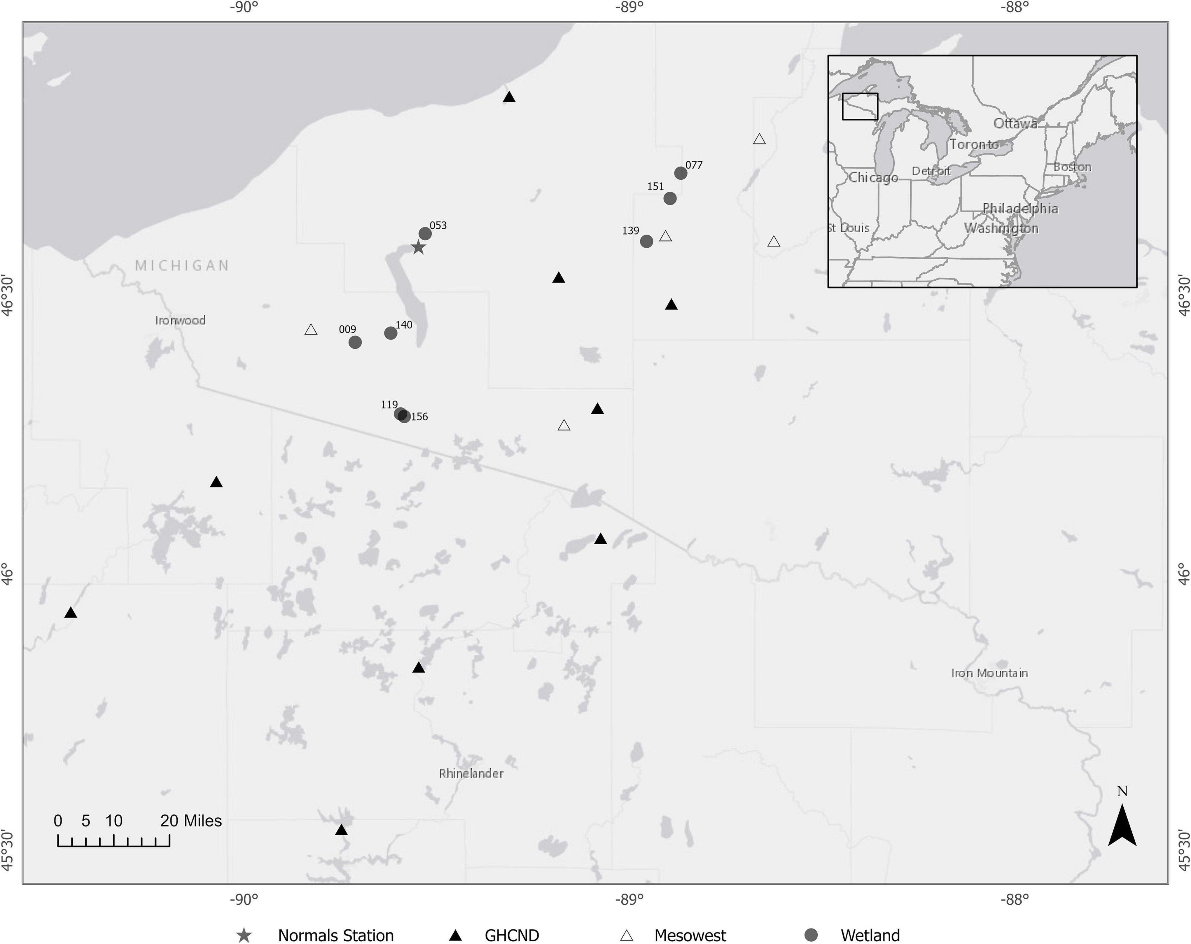
Figure 1. Map of study site and meteorological stations of Global Historic Climate Network—Daily (GHCND), Mesowest, and Norms Station used for data retrieval. Coordinates are in meters, UTM Zone 16N.

TABLE 1

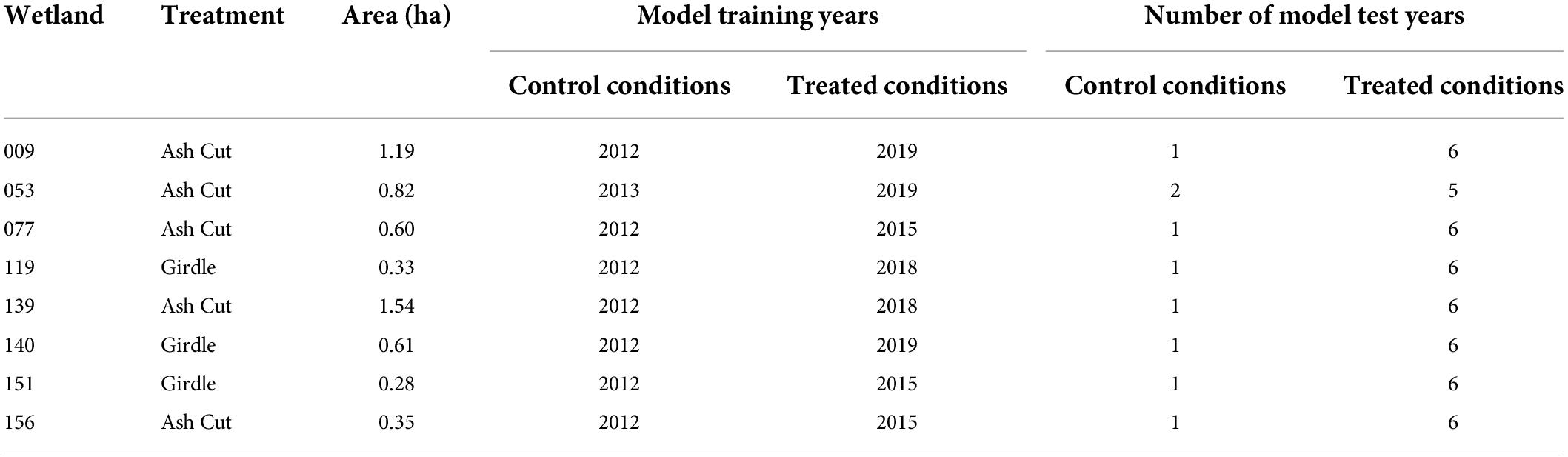
Table 1. Wetland size and treatment for field-study sites and 2012–2020 water year records used to develop wetland water level models.

Daily precipitation, daily minimum/maximum temperatures, and solar radiation observations were retrieved from existing meteorological stations. Daily precipitation and daily minimum/maximum temperature were used as inputs to the wetland water level models described below, and to derive daily solar radiation, potential evapotranspiration (PET), precipitation as snowfall and as rain, and snowmelt. Precipitation records were retrieved from the National Centers for Environmental Information Hourly Precipitation Dataset (Hourly Precipitation Data [HPD], 2021) and summed to daily values using the stations USC00201088 (Bruce Crossing, MI, United States), USC00204328 (Kenton, MI, United States), USC00475352 (Mercer Ranger Station, WI, United States), USC00206215 (Ontonagon, MI, United States), USC00476398 (Park Falls, WI, United States), USC00476518 (Phelps, WI, United States), USC00476939 (Rainbow Reservoir Lake, Tomahawk, WI, United States), USC00477140 (Rice Reservoir, Tomahawk, WI, United States), and USC00208680 (Watersmeet Fish Hatchery, Watersmeet, MI, United States) (Figure 1). Daily minimum and maximum temperatures were taken from the Global Historical Climatology Network (GHCND) dataset (Menne et al., 2012a,b) for the same stations, which were collocated stations for HPD and GHCND. Where data were missing, values were filled using inverse distance weighting using additional data retrieved from the Mesowest (Horel et al., 2002) network stations BPLM4 (Baraga Plains, MI), KTNM4 (Kenton, MI), PIEM4 (Pelkie, MI), WKFM4 (Wakefield, MI), WMTM4 (Watersmeet, MI). Solar radiation data were also retrieved from the listed Mesowest stations. The solar radiation and temperature data were used to fit the Bristow-Campbell method coefficients to estimate solar radiation from latitude and daily temperature range using the PIEM4 Mesowest site (Bristow and Campbell, 1984; Bojanowski, 2016). Bristow-Campbell solar radiation was used to calculate potential evapotranspiration (PET) via the modified Hargreaves-Samani equation (Hargreaves and Allen, 2003). Precipitation was partitioned into snowfall, rain, and snowmelt inputs using the CemaNeige snow accounting routine (SAR) (Valéry et al., 2014). The CemaNeige SAR is temperature-index based and accounts for accumulation, snowpack cold content, and snowmelt through a thermal state weighting coefficient and a degree-day melt coefficient. The CemaNeige SAR is implemented in the R package airGR (Coron et al., 2017).

Ecosystem specific yield

The link between hydrology drivers (rainfall, snowmelt, PET) and daily water level response has been shown to be non-linear and varying with stage (White, 1932; Loheide, 2008). In wetland systems the relationship between the driver magnitude and response magnitude has been termed the ecosystem specific yield (E_Sy) (McLaughlin and Cohen, 2014). E_Sy has previously been empirically derived as the ratio between precipitation inputs and water level rise ($\frac{P}{\mathrm{\Delta }WL}$) (McLaughlin and Cohen, 2014). The relationship between empirical E_Sy and water level can then be modeled to provide a continuous estimate of E_Sy. Models used to depict the relationship between E_Sy and water level include exponential (McLaughlin and Cohen, 2014; Watras et al., 2017), quadratic (McLaughlin and Cohen, 2014), and step-wise regression (McLaughlin and Cohen, 2014). Identifying E_Sy using the rainfall-rise ratio can be difficult in the presence of confounding hydrologic variation such as surface water connectivity and low-frequency seasonal changes in water availability (Zhu et al., 2011; Watras et al., 2017). Both factors were present in our study wetlands and there was no clear relationship that adequately represented the function relating $\frac{P}{\mathrm{\Delta }WL}$ and water level (Shannon et al., 2022), requiring an alternative approach. Shannon et al. (2022) developed an alternative using an inverse analog to $\frac{P}{\mathrm{\Delta }WL}$, deriving E_Sy from the ratio of cumulative water availability (Equation 1) and water level. The first step is to fit a quadratic curve to the relationship between a year-to-date water availability index from the beginning of the growing season (April 1st) to the point of minimum wetland water level (Supplementary Figure 1), where

$W{A}_{YTD}=P_{YTD}+M_{YTD}-PE{T}_{YTD},(1)$

and, WA_YTD, P_YTD, M_YTD, and PET_YTD are year-to-date water availability index, rainfall, snowmelt, and potential evapotranspiration, respectively. In developing this index, it is assumed that PET_YTD = cAET_YTD, where c is a constant representing a stable relationship between PET and actual evapotranspiration (AET). This assumption is supported by the hydrology of these wetlands, from spring through much of the growing season these sites are not water-limited (Van Grinsven et al., 2017). Empirical E_Sy was then considered as the first derivative of the curve, which has the form $\frac{\mathrm{\Delta }WL}{\mathrm{\Delta }WA}$, or the cumulative water level change per unit change in cumulative water availability. In the models described below, E_Sy is used to determine the actual water level change per unit of individual drivers [precipitation/snow melt/evapotranspiration (ET)]. This approach resulted in an asymptotic relationship between E_Sy and water level, suggesting agreement with the exponential forms in McLaughlin and Cohen (2014) and Watras et al. (2017). Defining E_Sy as $\frac{\mathrm{\Delta }WL}{\mathrm{\Delta }WA}$ provided additional data used in fitting the relationship between E_Sy and water level compared to the rainfall/rise method because it allows the use of days without rainfall in model development. Models for E_Sy were fit using the year with the greatest water level drawdown for each wetland to capture the widest range of E_Sy variation. Each wetland had the same basic form of E_Sy function. The functions were fit using a single hierarchical model with each of the coefficients allowed to vary independently within sites using the brms package in R (Bürkner, 2017, 2018). The structure of the E_Sy function requires that a lower bound be placed on E_Sy predictions to avoid values less than or equal to zero. The minimum value of E_Sy was determined as E_Sy at the wetland threshold water level (see “Wetland hydrology models” below).

Wetland hydrology models

Wetland water levels were simulated on a continuous basis using daily inputs. For each daily step, wetland water level change was determined as a function of the previous day’s water level, daily rainfall (R), daily PET, daily snowmelt (M), and estimated streamflow (Q) (Box 1 and Table 2). Threshold wetland water levels (WL_con) for surface water connectivity were estimated separately from the control and treatment period as the mode of the wetland water level record for the period. This is similar to definition of h_crit from McLaughlin et al. (2019) whose wetland surface water connectivity was also determined from wetland water level records. The initial water level for each year of simulation was set at WL_con, which assumes that dormant-season precipitation and snowmelt have filled the wetland basin to its maximum sustainable level. Streamflow was assumed to occur whenever wetland water levels were at or above the threshold water level. Each simulated daily water level step was used to estimate ${\widehat{E}}_{Sy}$, for the next day to serve as a multiplier for water level response to rainfall, PET, and snowmelt components. Each driver (R, PET, M, Q) has a coefficient (described in Table 2) allowing for wetland specific responses to meteorologic and physical drivers (fitting described below). β _AET adjusts PET to calculate estimated AET and β _–AET is the reduction in AET between the control and treatment periods. β _–AET controls for the change in AET after treatment when the black ash forest canopy was replaced by a shift to obligate- and facultative-wet herbaceous species (Davis et al., 2017). A first order autoregressive coefficient was also fit for precipitation to simulate slow-flow contributions to wetland water levels.

Box 1 Pseudocode representation of daily water level model implementation using variable definitions from Table 2.

TABLE 2

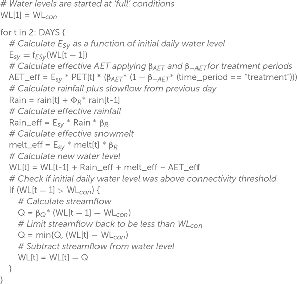
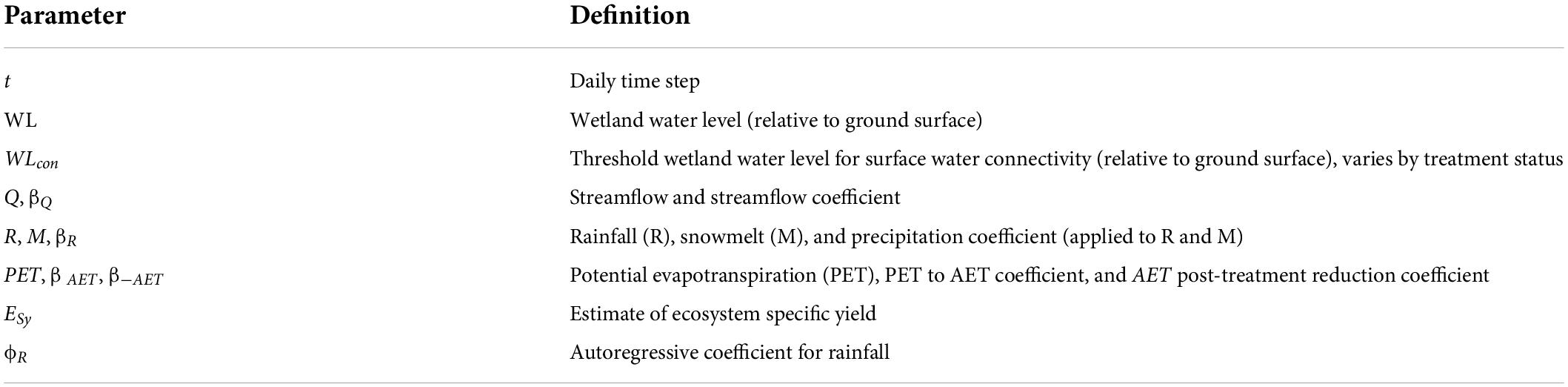
Table 2. Parameter notation and description for wetland water level models.

Training data for wetland water level models was selected for each wetland as the year with the greatest water level drawdown within each of the control and treatment periods, all other years of data from 2012 to 2020 were used for wetland model evaluation (Table 1). Wetland parameters were fit using a mixed effect modeling approach implemented as partial pooling of the population and individual wetland variance with the variational inference algorithm implemented in the probabilistic programming language Stan (Stan Development Team, 2022). Use of partial pooling reduced the potential to over-fit the individual wetland models to the training data available for each wetland. A joint model was fit to the control and treated conditions applying β _–AET to only treated data to reduce PET, while pooling fitting information between the control and treated conditions for all other parameters. This approach used data from both the control and treatment period to estimate the majority of the parameters, effectively doubling the available information for fitting. Wetlands with intermittent surface water connectivity show limited response to meteorologic drivers when above WL_con (McLaughlin et al., 2019). To account for the lack of response when wetland water levels were at or above WL_con, observation weights were adjusted asymmetrically during model fitting. Water levels at or above WL_con were given an initial 1/n weighting (identical to an unweighted model), but when water levels were below WL_con, the initial weights increased with the square of the difference between water level and WL_con. This weighting structure gave increased weight to the drawdown portions of the hydroperiod, reducing the impact of surface-flow related water level fluctuations around WL_con on model fitting. Median parameter estimates from the posterior distribution at the site-level were used in further analysis regarding model evaluation and simulation of future conditions. Parameter estimates and WL_con by treatment period can be found in Supplementary Table 1.

In addition to black ash and non-forested conditions, we simulated reforested black ash wetlands under one set of many potential future forest compositions. For the selected alternate-forest conditions, we assumed that a mix of the current co-dominant species, red maple and yellow birch, would become established with similar stand basal area as the present forests. Alternate-forested simulations were performed using the same parameters as the control period with a reduction of β _AET. This reduction is separate from the β _–AET term above, which is fit to observed data from non-forested conditions. The reduction of β _AET for alternate-forested conditions was a function of water level and current proportion of site basal area as black ash:

${\mathrm{\beta }}_{\text{A}\text{E}\text{T},\mathrm{alternate}-\mathrm{forest}}={\mathrm{\beta }}_{\text{A}\text{E}\text{T}}*[(1-B{A}_{\text{a}\text{s}\text{h}})+B{A}_{\text{a}\text{s}\text{h}}*$

${[1.45077-0.05869*(\mathrm{WL}-{\mathrm{WL}}_{\mathrm{con}})]}^{-1}]$

where, BA_ash is the proportion of wetland basal area represented by black ash. This equation is derived from previous work showing a water level-dependent difference in sap flux between black ash and current co-dominant species (Shannon et al., 2018).

Weather sequences under alternative climate scenarios

Future climate conditions were simulated by running wetland models under projected future (2070–2099) scenarios. For an unbiased comparison between current and future conditions, current climate scenarios are represented by hindcasted GCM historical climate scenarios (1980–2009) rather than observed conditions during the study period. Daily climate was projected for each combination of scenario (more sensitive GCM under higher forcing and less-sensitive GCM under lower forcing) and period (1980–2009, 2070–2099). Performance of GCMs in the North American Great Lake region varies mostly due to the unaccounted regional climate impact of the Great Lakes (Notaro et al., 2015; Rood and Briley, 2018). GCM model selection was guided by performance and sensitivity of the models to climate change in the Great Lakes region (Byun and Hamlet, 2018). Based on the results of Byun and Hamlet (2018), we chose to use the General Fluid Dynamics Lab Coupled Model (GFDL-CM3) and National Center for Atmospheric Research Community Earth System Model (CCSM4) GCMs downscaled by the localized constructed analogs method (LOCA) (Gent et al., 2011; Griffies et al., 2011; Pierce et al., 2014). LOCA downscaled data were retrieved from the downscaled CMIP3 and CMIP5 Climate and Hydrology Projections archive.¹ Both GFDL-CM3 and CCSM4 were shown to perform well for the Great Lakes region, and CCSM4 and GFDL-CM3 represent models that show less and more sensitive responses to a given RCP forcing, respectively [Figure 5 in Byun and Hamlet (2018)]. The two future climate scenarios used for simulations were the CCSM4 under RCP 4.5 and GFDL-CM3 under RCP 8.5. We refer to CCSM4 under RCP 4.5 as the warm & dry scenario with mean summer temperatures projected to increase 1.9°C and mean summer precipitation is projected to decrease by 2.6 cm relative to CCSM4 hindcasts of the 1980–2009 period. We refer to GFDL-CM3 under RCP 8.5 as the hot & wet scenario with mean summer temperatures projected to increase 8.9°C and mean summer precipitation is projected to increase by 6.2 cm relative to GFDL-CM3 hindcasts of the 1980–2009 period. Inspection of LOCA daily simulations of GFDL-CM3 and CCSM4 for the 1980–2009 period show excellent alignment with regionally observed conditions during the same period (Supplementary Figure 2). There appears to be fewer dry days in the LOCA dataset relative to the observed dataset. Monthly and seasonal precipitation totals showed good agreement between the LOCA and observed datasets and no bias-correction was performed.

The objective of simulating wetland conditions under climate scenarios is to understand the expected response and the range of possible responses. The 30-year periods of daily projections under LOCA downscaling provide a representation of the normal climate variation under each scenario (Baddour and Kontongomde, 2007). Quantifying the range of weather patterns under each climate scenario and the corresponding wetland response is best performed with many more years of simulation using stochastic processes (Wilks, 2012). While the LOCA downscaled-GCM data represents a model of physical processes, stochastic weather generators (SWGs) are statistical models used to generate additional weather series that are drawn from the distributions of the original modeled data. We followed the generalized linear model (GLM) based SWG with seasonal conditioning described in Verdin et al. (2015), which is a type of the more general Richardson SWG (Richardson, 1981). Details of SWG implementation can be found in the Supplementary Material Section “Stochastic weather generator–Methods.” Synthetic weather series of minimum and maximum temperatures, and precipitation were generated for all simulation data, and were used to calculate PET, snowfall, and snowmelt. The combination of SWG predicted synthetic series, and calculated values were used as inputs to the wetland hydrology models.

The LOCA-downscaled projected daily data from the coordinates of the Bergland Dam meteorological station were used to fit SWGs for each climate scenario. Each SWG was used to simulate 10,000 individual annual synthetic weather series with seasonal conditioning drawn randomly from the 30 years of projection data. Conditioning the models on individual years of observed data is intended to increase interannual variability, which can otherwise be limited in SWGs (Wilks and Wilby, 1999).

Data analysis

Results of this research consists solely of simulation data to draw conclusions from modeled wetland water levels driven by synthetic weather series generated from parametric descriptions of LOCA downscaled GCM projections. To avoid a false sense of dichotomy about the future climate and wetland conditions, we report our results by contrasting the probability of observing certain wetland conditions under different vegetation types and climate scenarios and account for the uncertainty inherent from these simulations by including the entire the distribution of simulation results (McElreath, 2020). This means that tests for statistical significance are not presented for most analysis results, but rather effect sizes are compared. As an exception, the performance of water level models is evaluated using a mixed-effects linear model to demonstrate no statistical difference between observed and modeled water levels. All simulation and analysis were carried out using the R statistical computing language (R Core Team, 2019).

Future hydrologic conditions

Observed water levels from 2012 to 2020 within these wetlands show high interannual variation under field control and treatment conditions. Rather than considering this low-signal, high-variance variable, we expand the concept of WL_con and define three critical ecohydrological thresholds (CEHTs) to a measure the impact of vegetation and climate changes. CEHTs were set to capture wetland connectivity to the downstream hydrologic network via streamflow and subsurface flow, inundation when wetland water levels were at or near the soil surface with surface water likely in microtopographic hollows, and drawdown when wetland water levels dropped far below the surface of the wetland (Table 3). Wetland water table levels were compared to these thresholds and the number of days that a wetland was above or below a given threshold could be used to calculate the probability of occurrence of that CEHT. We chose to calculate and compare these probabilities at the monthly scale, though they could be computed for other time scales from daily to annually.

TABLE 3

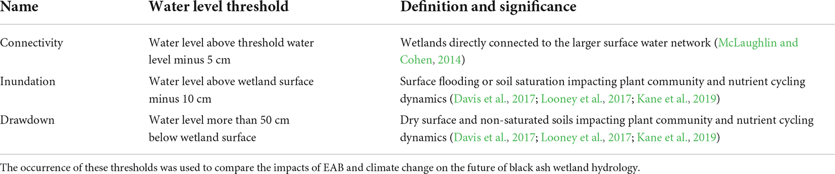
Table 3. Water level thresholds and definition of three conditions considered as critical ecohydrological thresholds.

Wetland model performance

Wetland water level model performance was evaluated using the retained independent testing datasets (all years 2012–2020 not included as training years in Table 1). Model performance was assessed using observed meteorologic conditions, in contrast to simulation results, which relied on hindcast climate conditions. We calculated R² as a metric for the relationship between observed and modeled values. R² cannot be used to evaluate the accuracy of the models because consistent over- or under-predictions can still result in high R² values (Krause et al., 2005). The median error of daily modeled water level was used to measure model bias and the root median squared error (RMedSE) of the daily modeled water level to assess overall predictive accuracy. RMedSE was used in place of RMSE because we expect some outlier errors where regionally-informed local rainfall records do not match actual rainfall within study wetlands. Relative RMedSE was calculated as the RMedSE relative to the observed annual range in daily wetland water levels to provide additional context on the scale of the errors. In addition to the overall accuracy of the models, we want to accurately capture the probability of occurrence of the CEHTs. We tested the predicted probabilities of inundation, connectivity, and drawdown to the observed probabilities of the same conditions using a linear mixed effects model with dependent variable as the probability of occurrence, population effects of observed/predicted and wetland status, and a group effect for wetland (Lenth, 2021). Summary and statistical tests were performed using estimated marginal means (Bates et al., 2015). Directly proving the theoretical basis of the approach used to calculate E_Sy is outside the scope of this study and would be best performed with a purpose-designed experiment or simulation. To assess the application of the approach, we compare quantile regressions (τ = 0.5) between the daily water level change and WA_YTD (Equation 1) using adjusted (the product of driver and E_Sy) and unadjusted (no E_Sy) drivers.

Partitioning impacts between sources

Comparisons of the combined and separate impacts of EAB and climate change were performed against modeled baselines rather than field-study observed conditions. Comparing to modeled future simulated baselines with each alternative vegetation condition ensures that comparisons are not biased by the relationship between wetland meteorology and SWG weather sequences, avoiding the potential of identifying model artifacts as meaningful when comparing observed and modeled results. The distribution of modeled wetland water levels was evaluated for each future vegetation and climate scenario combination. The 10,000 simulations for each combination were summarized by simulated day of year to compute the median and the 67% highest density credible intervals (HDCIs) (McElreath, 2020) for each combination. HDCIs are potentially asymmetric intervals that contain the stated proportion of all observations. They differ from confidence intervals by providing information about the most probable range for results rather than identifying the range of values that would be expected to contain the true mean. This approach was used to quantify future conditions and baseline scenarios for comparison and benchmarking. Modeled baselines provide consistency between the baseline, or control, period and alternative vegetation cover and climate scenarios, which is critical for drawing meaningful conclusions. Apart from the advantage of consistency, modeled baselines can also provide a flexible tool to answer more questions about the drivers of the observed changes. Different baselines can be computed from the simulations by combining the six vegetation-climate combinations. To evaluate total impact of EAB and climate change, future non-black ash conditions were compared to black ash under the current climate. Alternative baseline comparisons included comparing each vegetation cover to itself under alternative climate scenarios, and comparing vegetation covers to each other within a climate scenario. These two alternative baselines allowed us to determine how much of the observed total impact was attributable to either climate projects or EAB using the same set of 10,000 simulations.

Results

Ecosystem specific yield

The results of a quantile regression of pooled data (used only to validate E_Sy development but not used elsewhere in this study) explain daily change in wetland water level as a function of PET, P, and M (Equation 1 and Figure 2). We found that pseudo-R² of the model improved from 0.63 to 0.74 when the product of the inputs and modeled ecosystem specific yield are used. The difference between pseudo-R² is large enough to be of note, but more importantly we can see that water level drawdown is extremely underestimated by the unadjusted model (Figures 2A,B). Our results show that periods with the highest drawdown are not correctly modeled using the raw inputs. Prediction is improved during these periods of high drawdown when the E_Sy adjusted hydrologic inputs are used. Periods of high drawdown generally occurred mid-season when water levels were farther below the surface, corresponding to higher expected E_Sy estimates.

FIGURE 2

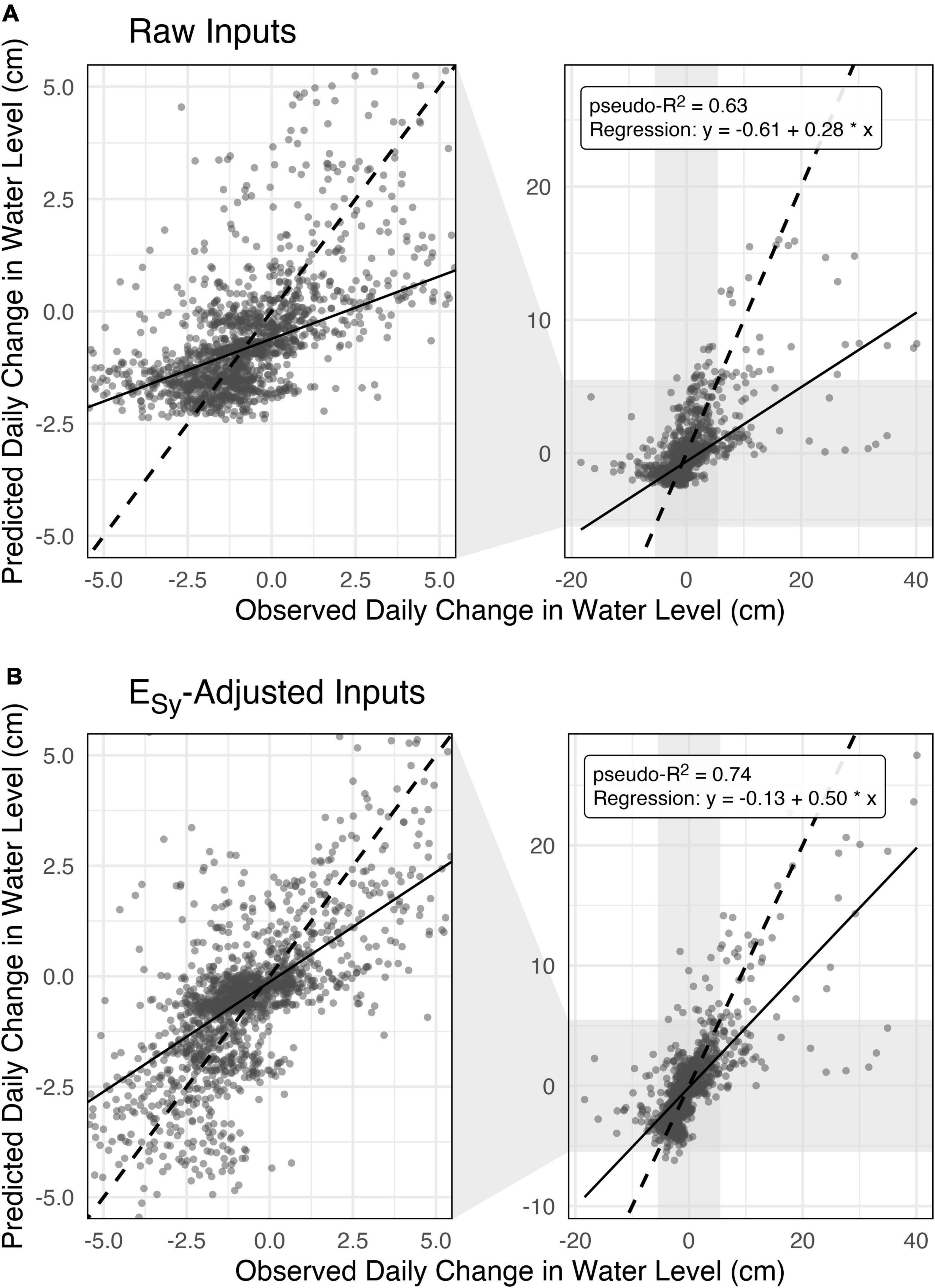
Figure 2. Predictions of daily change in water level using a quantile regression with observed daily water level as the dependent variable and potential evapotranspiration (PET), rainfall, and snowmelt as the independent variables. The model was fit two times, once with raw hydrologic inputs (A) and once with inputs adjusted by ecosystem specific yield (B). The right panels show the full dataset while the left panels zoom in on an interval [-5, 5] for both the observed and predicted water levels. The dashed line shows a 1:1 line and the solid line shows a quantile regression (τ = 0.5) between predicted and observed water levels.

Wetland water level model performance

Wetland water level models performed well for most wetlands with median errors between 0 and −10 cm, R² of 0.75–0.90, and RMedSE values of less than 7.5 cm (Figure 3B). Predicted water levels at two wetlands, 119 and 156, had R² below 0.6 for most of the withheld training years, which was chosen as a threshold for unsatisfactory model results based on work by Moriasi et al. (2015). Models at these wetlands showed similar rates of bias or error relative to the other wetlands. Both of these sites are closed basins with no surface outlet and site 119 was shown to have different source water characteristics from other sites, showing much less connectivity to groundwater sources (Van Grinsven et al., 2017). Site 053 had good correlation between predicted and observed water levels, but variable performance on the magnitude of predictions (Figures 3A,B). Mean and median model performance was similar for both control and treatment conditions for all model metrics (Supplementary Table 2). Median errors less than zero show that the models had an overall negative bias, which indicates drier simulated wetland conditions than were observed (Figure 3A). The median rRMedSE is moderate for both Control and Treated condition models (∼15%), but notable outliers were present at wetlands 053 and 077 (Figure 3D and Supplementary Table 2).

FIGURE 3

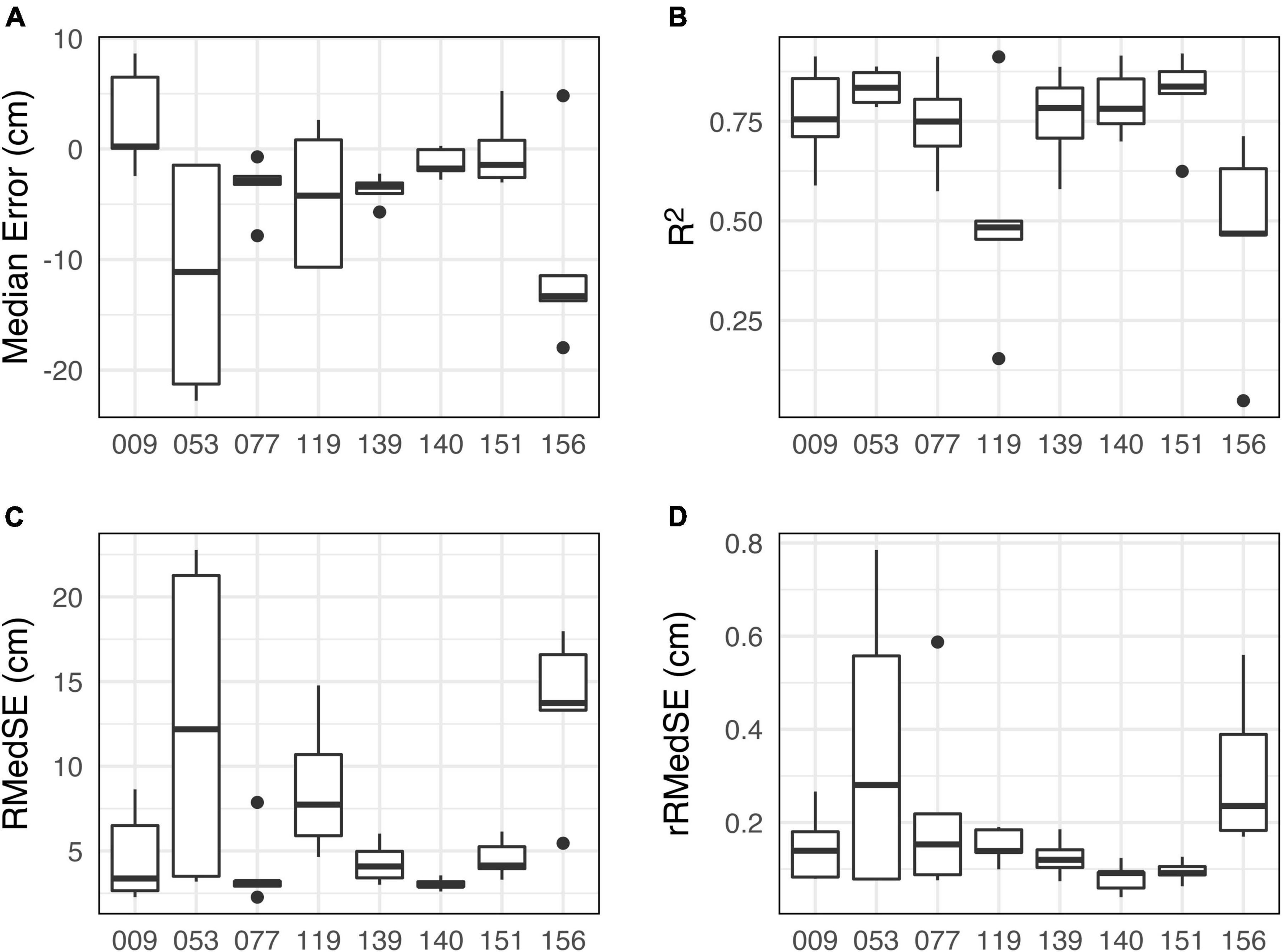
Figure 3. Wetland model performance metrics. Individual metrics were calculated for each site-year combination for all withheld test years (control and treatment conditions) and are presented within sites. Evaluated metrics include median error (A), R² (B), root median squared error (RMedSE, C), and root median squared error relative to the annual range of daily wetland water level within that year (rRMedSE, D).

When compared to observed wetland water levels, modeled wetland water levels showed no significant (α = 0.05) difference in probability of occurrence of CEHTs (Figure 4 and Supplementary Table 3). The range of site-level probability of each level of interest was similar between modeled and observed data (Figure 4). Though not significant, these results show a slight systematic bias toward drier conditions in the modeled wetland water levels. This bias was consistent for both the control and treatment conditions. All remaining comparisons of current conditions to combinations of future vegetation conditions and climate scenarios use modeled current conditions and not observed current conditions. This comparison ensures that the described model bias does not impact results, but it does create a disconnect between observed conditions and expected changes.

FIGURE 4

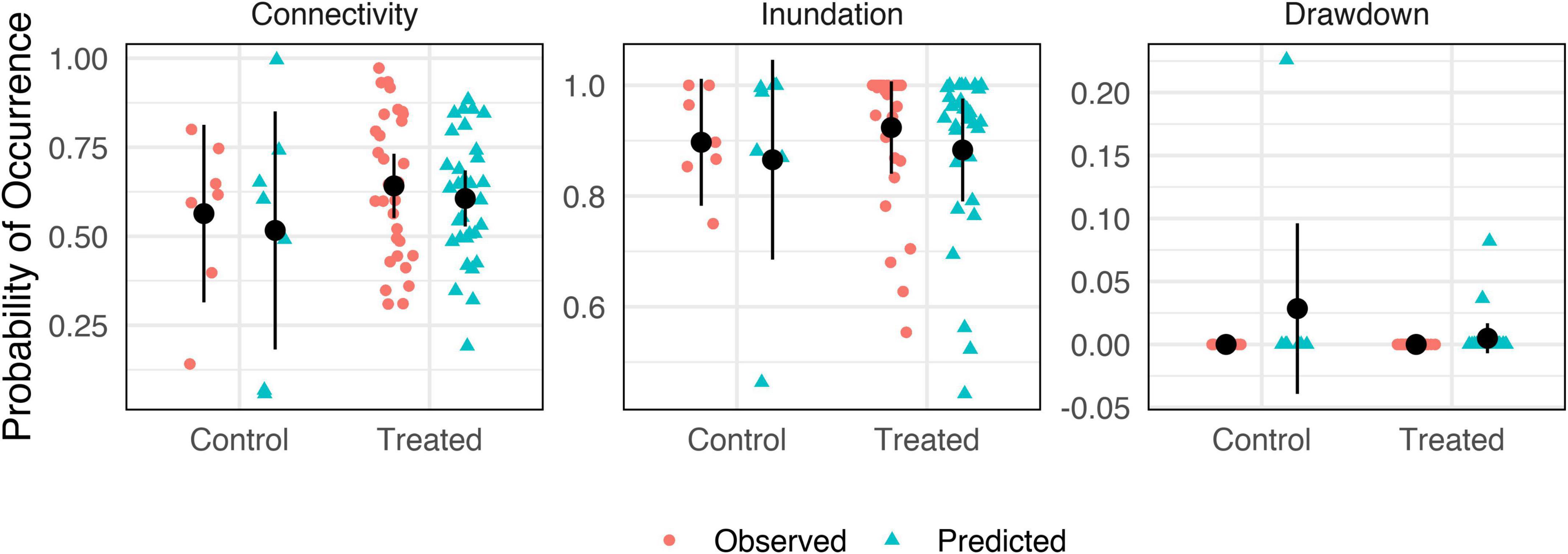
Figure 4. Tests comparing predicted probability of occurrence for critical ecohydrological thresholds (CEHT). Reported values show the seasonal probability of daily water level exceeding the respective CEHT. Control and treated conditions refer to observed control and treated conditions or predicted modeled black ash and modeled non-forested conditions. Black point and error bar represent estimated marginal mean and its 95% confidence interval. Individual points represent data observed or simulated for 1 year at one site. All data presented were derived only from the withheld test period for each wetland.

Future hydrologic conditions

Synthetic weather generators were shown to be representative of the LOCA downscaled data (Supplementary Material Section “Stochastic weather generators–Results”). Changes in wetland water levels under future climate conditions were highly variable across both scenarios and both vegetation types (Figure 5). The reported probability is the proportion of observations where daily water level surpasses each threshold out of all modeled daily water levels in a month (∼240,000). The median probability and a range representing 67% of all observations (highest density continuous intervals, HDCI) are shown as point and line estimates for the warm & dry and hot & wet future climate scenarios. Modeled black ash conditions are also reported as the median and 67% HDCI, represented as a crossbar and shaded area.

FIGURE 5

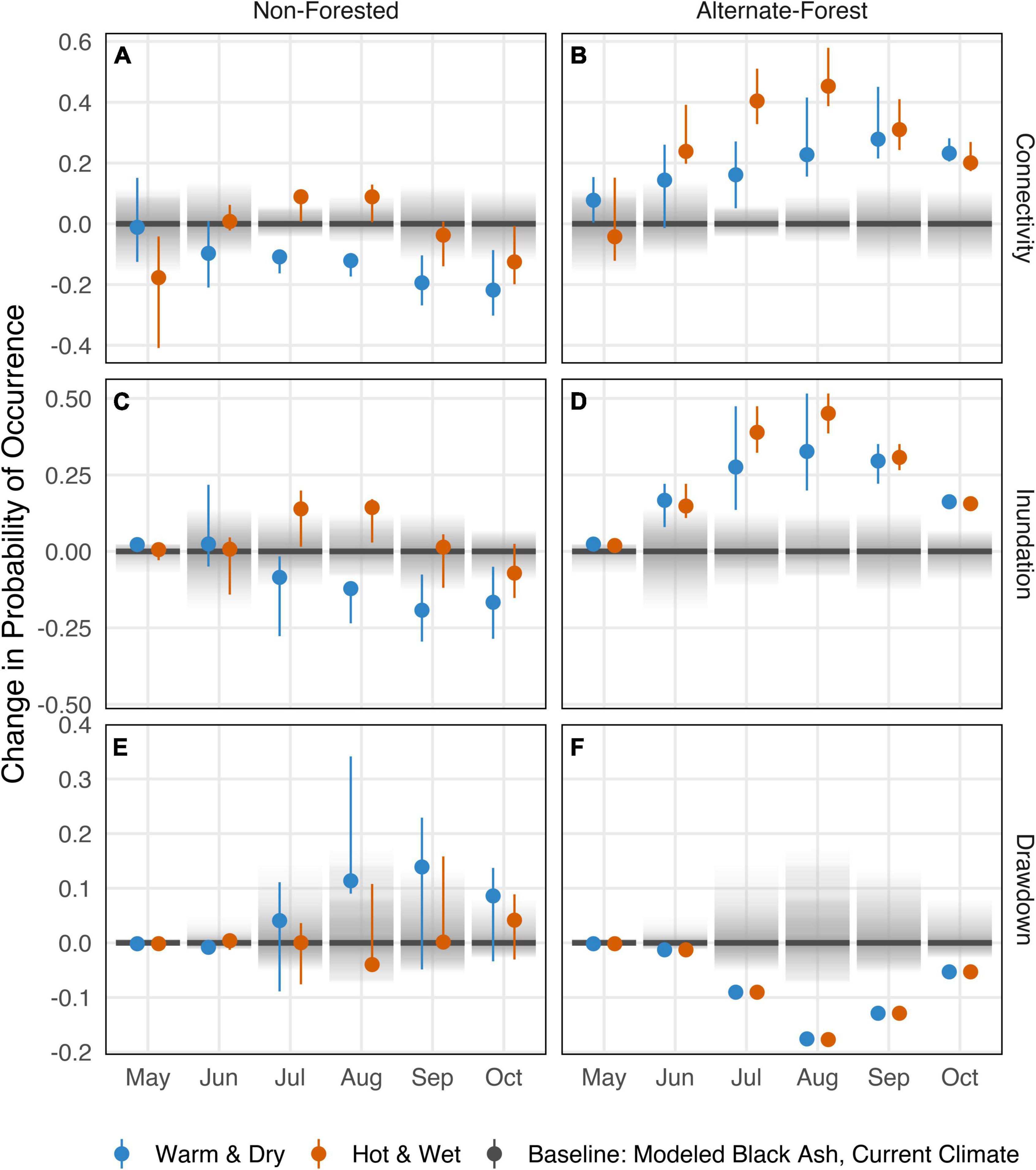
Figure 5. Change in probability of water levels above (connectivity, inundation) or below (drawdown) ecohydrologically significant thresholds (CEHT) under future vegetation (non-forested or alternate-forested) and climate scenarios relative to baseline of black ash under a current climate where each combination of CEHT and future vegetation condition is identified in panels (A–F). Probability of occurrence is the proportion of days in each month that simulated water levels reached and exceeded each threshold. Values are reported as the median (point/bar) and the bounds of a 67% highest density continuous interval (HDCI, an interval, potentially asymmetric, that contains 67% of simulated values). For some combinations of vegetation conditions and climate scenarios the HDCI may be indistinguishable from the point estimate because of the small range covered by the HDCI. Blue and orange colors represent warm & dry and hot & wet future climate scenarios, respectively. Gray shaded area represents 67% HDCI of model simulations for control black ash conditions under the current climate (baseline condition) and the black crossbar represents the baseline monthly median probability (centered to zero).

For non-forested conditions, the results of both climate scenarios primarily showed a decrease in probability of connectivity relative to current wetland conditions, except for the hot & wet scenario in June, July and August, which showed an increased probability of connectivity (Figure 5A). In July, August, September, and October, the warm & dry climate scenario consistently showed wetlands as drier than current conditions: lower median probabilities of connectivity and inundation, higher probability of drawdown, and little-to-no overlap with the HDCI of current conditions (Figures 5A,C,E). The hot & wet climate scenario showed slightly wetter wetlands in July and August, connectivity (+), inundation (+), drawdown (−) than current conditions, though there is considerable overlap between future and current climate scenarios. Alternate-forested conditions were consistently wetter than current conditions under both climate scenarios, with a significant increase in connectivity and inundation and decrease in drawdown, particularly during July-September period (Figures 5B,D,F). Changes to wetland hydrology were consistently wetter under the alternate-forested conditions and both climate scenarios, while the non-forested conditions showed variable results between the two climate scenarios. Currently these wetlands have a hydroperiod with high water levels in May at the start of the growing season, a drawdown period of variable strength, and then a rapid rebound in water levels at the end of the growing season mid-September to October. Increased June-August connectivity and inundation in the alternate-forested conditions under both climate scenarios and the non-forested conditions under the hot & wet scenario show dampening of that hydroperiod trend. On the other hand, non-forested conditions under the warm & dry scenario showed an amplification of the current hydroperiod, with drawdown increasing and connectivity/inundation decreasing through the growing season and not rebounding until October or later (Figures 5A,C,E).

Within a given vegetation condition, inundation results in Figures 5C,D closely resemble the patterns observed in the connectivity results in Figures 5A,B. This is in line with fit model parameters that showed maximum sustained water levels were above the surface for almost every wetland and treatment combination (Supplementary Table 1). For connectivity/inundation, the non-forested conditions under the hot & wet climate scenario showed more overlap with current conditions than the warm & dry scenario (Figures 5A,C). This is in contrast to the alternate-forested conditions, where the hot & wet scenario showed a larger increase in probability of connectivity/inundation (Figures 5B,D). Under both climate scenarios the alternate-forest conditions showed a lower probability of drawdown than under baseline conditions, with almost no overlap with current conditions from July through October (Figure 5F). Drawdown events were very unlikely with near zero probability of occurring under alternate-forested conditions under both climate scenarios. Probability of drawdown in non-forested conditions increased in both magnitude and variability in August and September under the warm & dry future climate scenario, and increased in variability in the same period under the hot & wet future climate scenario. Differences from current conditions were greatest in August under the warm & dry climate scenario (Figures 5E,F).

Partitioning driver impact

To isolate the impact of climate change, we compared the simulations under the current climate to simulations under future climate scenarios for each vegetation class (black ash forested, alternate-forested, and non-forested) condition (Figure 6). To isolate the impact of changes to vegetative cover driven by EAB, we compared the simulations of the black ash forested class to simulations of alternative vegetation conditions, including the alternate-forested and non-forested condition classes, for each climate scenario (Figure 7). Climate impacts were similar for black ash and non-forested conditions under both future climate scenarios, with decreasing connectivity/inundation and increasing drawdown (Figure 6). Alternate-forested conditions show much less change under both future climate scenarios compared to simulations under the current climate (Figure 6). We also found that under current climate scenarios, non-forested conditions were closer to baseline black ash conditions under the same climate scenario than alternate-forested conditions (Figure 7). However, under future climate scenarios both non-forested and alternate-forested conditions showed little agreement with black ash wetland conditions and were consistently more likely to have connected and/or inundated conditions and less likely to see drawdown below 50 cm (Figure 7).

FIGURE 6

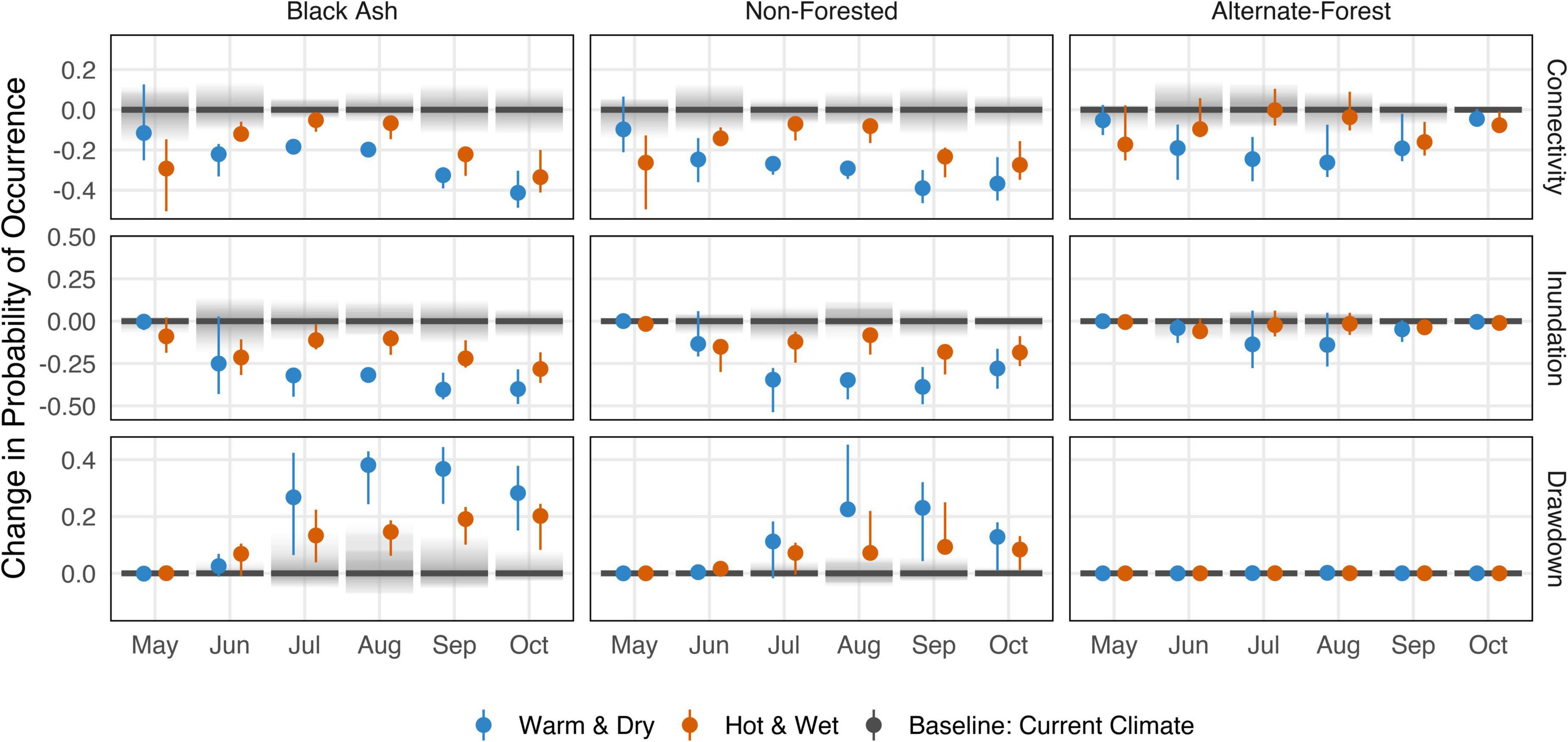
Figure 6. Change in probability of occurrence for critical ecohydrological wetland water levels (connectivity, inundation, drawdown) under combinations of vegetative cover (black ash, alternate-forested, non-forested) and climate conditions (warm & dry, hot & wet) relative to the respective vegetative cover under current climate baseline. Each column compares simulated wetland response within a fixed vegetation condition across multiple climate scenarios. Values are reported as the median (point/bar) and the bounds of a 67% highest density continuous interval (HDCI, an interval, potentially asymmetric, that contains 67% of simulated values). For some combinations of vegetation conditions and climate scenarios the HDCI may be indistinguishable from the point estimate. Blue and orange colors represent warm & dry and hot & wet future climate scenarios, respectively. Gray shaded area represents HDCI of modeled baseline.

FIGURE 7

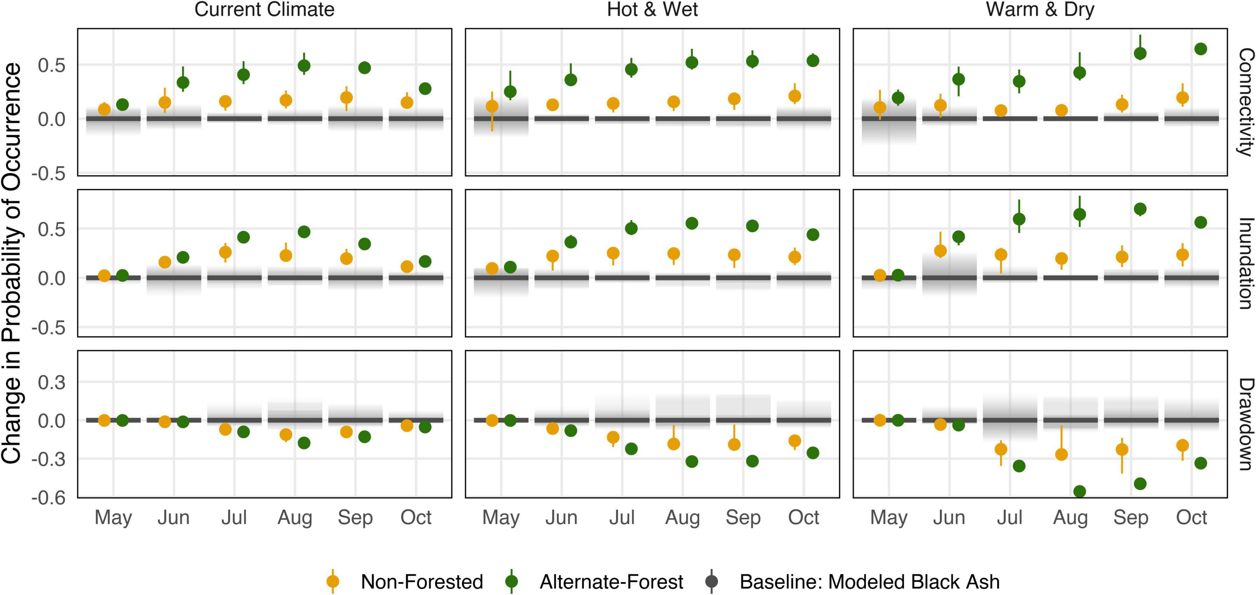
Figure 7. Change in probability of occurrence for critical ecohydrological wetland water levels (connectivity, inundation, drawdown) under combinations of vegetative cover (black ash, alternate-forested, non-forested) and climate conditions relative to the respective climate scenario (warm & dry, hot & wet) under black ash cover. Each column compares simulated wetland response within a fixed climate scenario across multiple potential vegetative covers. Differences within a column represent the impact of EAB and potential management decisions. Values are reported as the median (point/bar) and the bounds of a 67% highest density continuous interval (HDCI, an interval, potentially asymmetric, that contains 67% of simulated values). For some combinations of vegetation conditions and climate scenarios the HDCI may be indistinguishable from the point estimate. Green and yellow colors represent alternate-forested and non-forested vegetation conditions, respectively. Gray shaded area represents HDCI of modeled baseline.

The direction of impact due to EAB-induced vegetation change is the opposite of both climate scenarios for both vegetation conditions (Figure 8). The impact attributable to vegetation change to non-forested conditions is of similar magnitude as the impact attributed to climate changes, but the alternate-forest scenario has a larger magnitude impact than the climate impact under either future climate scenario (Figure 8). The entirety of the decrease in the probability of drawdown under alternate-forested conditions is attributed to vegetation change (Figure 8).

FIGURE 8

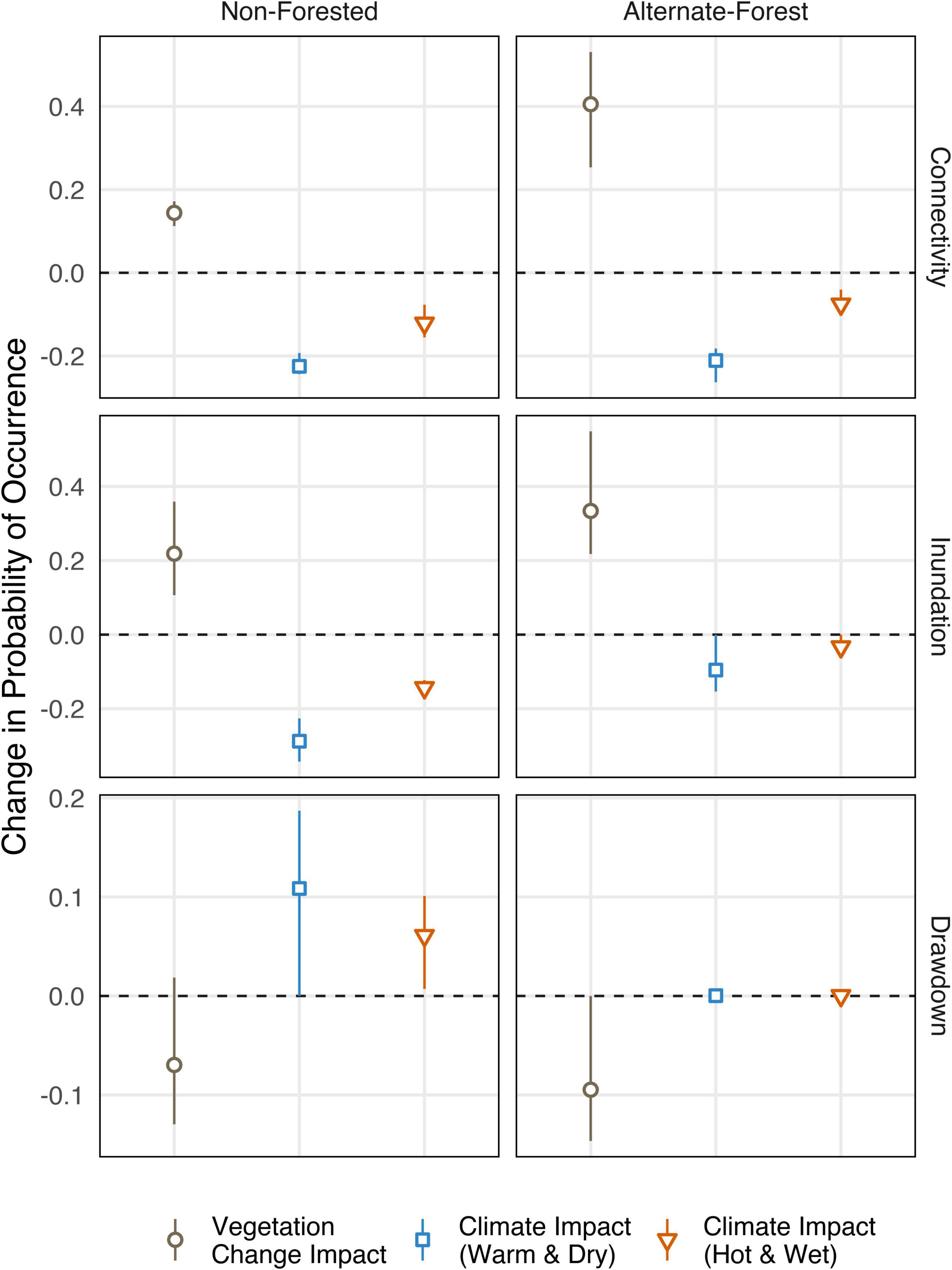
Figure 8. Expected change in probability of occurrence for critical ecohydrological water levels that can be attributed to future climate scenarios or vegetation change due to emerald ash borer (EAB) impact and management response. Vegetation impact values represent the difference between simulated black ash forests and each alternative vegetative condition under current climate conditions. Climate impacts represent the difference between each alternative vegetative condition under the current climate and future climate (warm & dry or hot & wet) scenarios. Differences are calculated using the daily values from July through September, highlighting growing season impacts. Values are reported as the median (point) and the bounds of a 67% highest density continuous interval (HDCI, an interval, potentially asymmetric, that contains 67% of simulated values). For some combination of vegetation conditions and climate scenarios the HDCI may be indistinguishable from the point estimate.

Discussion

Ecosystem specific yield

The approach used to calculate E_Sy, relating the magnitude of water level change to the drivers of that change, was adapted from and provides an alternative to approaches used to calculate E_Sy presented in previous research (McLaughlin and Cohen, 2014; Watras et al., 2017). The results of our comparison agree with others (McLaughlin and Cohen, 2014; Watras et al., 2017) who found that the impact of E_Sy increases as water levels decreased and that flooded conditions approach an E_Sy of 1 (Supplementary Figure 1). This relationship results in the largest adjustment to inputs during mid-season periods, explaining the differences observed between Figures 2A,B. Shannon et al. (2022) demonstrated that ET estimates derived using this approach perform comparably to other methods for calculating E_Sy (Soylu et al., 2012; McLaughlin and Cohen, 2014; Watras et al., 2017). Those results showed that calculated ET was correlated with daily PET estimates from nearby meteorological stations. Our results here together with those in Shannon et al. (2022), showing general agreement with the rainfall/rise method, provide empirical evidence that this alternative formulation captures the variation of E_Sy with wetlands. Thus, this alternative method can be used in scenarios where the rainfall-runoff ratio approach is masked by outside influences such as low-frequency hydrologic signals (Zhu et al., 2011) and surface water connectivity (Watras et al., 2017).

Wetland models

Wetland water level model performance provided reliable results to observe changes in the hydrographs of black ash wetlands and compare the probability of occurrence for CEHTs. The models showed good correlation between observed and modeled water levels (Figure 3A and Supplementary Table 2). The two wetlands with the lowest performance had the least responsive wetland water levels, remaining consistently inundated, suggesting that from both absolute and relative standpoint, the wetland models as developed captured wetland water levels more accurately for wetlands with greater variation in annual wetland water levels. Wetland model performance decreased sharply when wetland water levels were above WL_con, which is expected based on the lack of stream-gage results. We believe this issue has no impact on our results as analysis did not require daily water depth accuracy, but instead focused on the probability of exceeding WL_con as one of the CEHTs. Improving this component of the model would have required a combination of streamflow measurements during surface water connectivity or an approach analogous to separation of baseflow and quickflow in streams. Some wetlands (e.g., 053) showed high variability in performance during the test period (Figure 3). We believe much of this variability can be attributed to the use of off-site meteorological data during model evaluation. Storm systems, especially convective rain events in the growing season, can be highly variable over short distances (Osborn et al., 1979), such that off-site meteorological data may miss (or include) storms that are important to restoring wetland water levels in the summer. Additionally, wetland 053 was uniquely positioned on the landscape (along a ridge top) and therefore may have had different groundwater connectivity and flow dynamics than the other wetlands in this study.

Importantly for our conclusions, the wetland models performed well in predicting the probability of occurrence of CEHT levels. The probability of occurrence of connectivity, inundation, and drawdown was found not to be different between the observed and modeled data in the test periods (Figure 4 and Supplementary Table 3). Also, there is no significant systematic model bias (positive or negative) in the probabilities. Although no significant systematic model bias was identified for CEHT analysis, Figure 4 does indicate a bias toward drier simulations when daily water level measurements are compared. Therefore, the use of a modeled control baseline is an important safeguard against drawing conclusions from potential model artifacts. Comparing the systematically-biased results could exaggerate or mask the real expectation of wetter or drier wetland conditions.

Future hydrologic conditions and drivers

These simulation results aim to help relate potential future conditions to current conditions in dry, wet, or “normal” years. This work allows researchers and managers to answer questions such as: What will these sites look like in a “normal” year in the future? How will these sites respond to wet/dry conditions in the future? For example, we could expect that during a “normal” (median) year under the hot & wet future climate scenario a non-forested wetland on these sites would have a similar probability of surface inundation as a black ash wetland does today in a wet year (higher end of HDCI) (Figure 5C). In general, black ash wetlands that remain forested under potentially less inundation-adapted species can be expected to have wetter conditions relative to today under each of our simulated climate conditions. Each combination of climate and vegetation scenario can be used to influence management approaches and timing in responding to EAB in black ash wetlands.

The combined impact of EAB and climate is shown as the difference between future climate conditions and black ash conditions under historical climate (Figure 5). We were able to draw additional information about the individual effects of future climate and vegetative cover on wetlands by altering how we calculated the baseline. We found that EAB impacts lead to slightly wetter conditions under non-forested conditions and the present climate (Figure 7). This result agrees with observed water level response analysis in Van Grinsven et al. (2017), where absolute water level response to simulated post-EAB conditions resulted in wetter conditions and significantly lower growing season drawdown rates. A modeled alternate forest composition (alternate-forested) shows that EAB impact alone would lead to dramatically wetter conditions following invasion and death of black ash (Figure 7). This result is expected as we modeled our alternate-forested conditions based on previous work showing that co-dominant hardwoods had significantly lower seasonal transpiration estimates than black ash (Shannon et al., 2018). Under non-forested conditions, we found that the isolated impact of future climate scenarios would lead to much drier sites (Figure 6). Connected/inundated conditions would be less prevalent under non-forested conditions than the alternate-forested conditions. The probability of surface water connectivity or inundation occurring are dramatically decreased under both climate scenarios and the probability of wetland water levels dropping below 50 cm increases under non-forested conditions (discussed below in Reduced Evaporation and Non-Canopy Transpiration). Alternate-forested conditions show no change in the probability of drawdown relative to current conditions, and only slight decreases in connectivity and inundation under the warm & dry scenario (Figure 6), indicating the vegetation change to alternate-forested swamps the impact of future climate scenarios (Figure 8). The probability of each CEHT is not symmetrical around the median, indicating that for each comparison it is important to note if the conditions are likely to be wetter or drier than looking at the median alone would suggest (Figures 5–7).

Our hypothesis that EAB and climate change would counteract each other is supported by our results showing total impacts on non-forested conditions are often within the HDCI of current conditions (Figure 5). The dynamics of wetland water levels are complex and climate change and invasive species can each have major consequences (Burkett and Kusler, 2000; Moomaw et al., 2018). In summarizing our findings, we expect that wetlands that transition from black ash forests to non-forested sites become wetter, but the effects of increased summer evaporative demand will balance the wetter conditions over time (Figure 5 and Supplementary Figure 4). Our synthetic weather series indicated less summer precipitation under the warm & dry scenario, while under the hot & wet scenario we observed an increase in large storms (Supplementary Figure 4). If management or natural regeneration leads to establishment of future forests with lower site transpiration rates, the probability of high-water conditions in these wetlands can be expected to remain stable or increase in frequency, while dry conditions (water levels more than 50 cm below the surface) become rarer (Figures 5–7). Under both vegetation conditions, the warm & dry climate scenario resulted in a lower probability of connectivity relative to the hot & wet climate scenario (Figure 5), suggesting that in these systems the decrease in precipitation under the warm & dry scenario has a stronger influence than the increased evaporative demand of the hot & wet scenario. Our results also suggest that the impact of climate change alone in this region will lead to consistently drier conditions in most types of wetlands (Figure 7).

Future climate

The future climate scenarios used in this study represent future conditions under a less (warm & dry) or more (hot & wet) sensitive future climate conditions (Swanston et al., 2016). The warm & dry scenario summer is projected to be slightly drier than observed conditions, with similar PET (Table 4). When summer water deficit is calculated as P-PET, we see that, within a given year, conditions will show a decrease in water availability. The hot & wet scenario is a much wetter projection than both the observed climate and future warm & dry climate (Table 4). There is little to no overlap in the 67% HDCIs for summer precipitation between the hot & wet and other scenarios. However, a commensurate increase in summer evaporative demand may lead to only slightly wetter summer conditions under the hot & wet scenario. Spring and early summer water levels are currently strongly influenced by the snowfall and melt regimes (Van Grinsven et al., 2017). The Great Lakes region, including our study area, is expected to see less precipitation as snowfall and earlier snowmelt (Byun and Hamlet, 2018). This shift will result in spring melt becoming disconnected from the start of the growing season. Annual water deficits within these wetlands will be larger than the growing-season only water deficits in Table 4.

TABLE 4

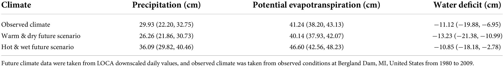
Table 4. Summer June/July/August precipitation, potential evapotranspiration, and water deficit (P–PET) for the climate scenarios in this study. Reported values are the median and bounds of the 67% highest density continuous interval of seasonal total precipitation by observed or projection year.

Each of our 10,000 simulations were run as individual years which results in no simulated long-term droughts and wet spells. We deliberately chose to use single-year simulations because of the length of available training data. During our study, the region was in the process of transitioning from a relatively dry period to a relatively wetter period (Supplementary Figure 5). Our training data are primarily drawn from the drier portion of the study period. Without longer-periods of training data we did not capture both the intra- and inter-annual dynamics of wetland hydrology. If we assumed all 10,000 years of synthetic weather series were contiguous weather records, the longest period of drought years (annual precipitation less than annual PET) was 7 and 9 years for the warm & dry and hot & wet climate scenarios, respectively. By using single-year simulations we are implicitly assuming that fall and winter (SON and DJF) precipitation is high enough to recharge the local hydrology driving these wetlands, restarting the cycle at or near maximum wetland water levels. When we consider only fall and winter precipitation, we found 0, 8.7, and 10.1% of synthetic weather series had totals below the tenth percentile of observed data, warm & dry, and hot & wet climate scenarios, respectively. Synthetic (and LOCA) winters were wetter than observed winters, supporting the assumption that dormant-season precipitation would be enough to recharge wetland water levels.

Interaction of actual evapotranspiration and ecosystem specific yield

It is expected that vegetation conditions with lower transpiration rates have lower rates of water level drawdown and therefore increased water levels. In these wetlands this effect is compounded by the dynamics of E_Sy. E_Sy increases in magnitude as water levels decline (Supplementary Figure 1B), which is the result of reduced soil pore space and wetland geometry where a smaller volume of change results in a large water level difference as effective wetland area decreases with wetland water level (McLaughlin and Cohen, 2014). The effect is that the same AET results in smaller changes to wetland water levels under wet conditions than dry conditions. In this way the impact of EAB may result in a feedback loop in which water levels remain elevated:

1. Actual evapotranspiration begins to draw down water levels, E_Sy is low,

2. Water levels decline slowly because of reduced AET and low E_Sy,

3. At the peak of the growing season, E_Sy is lower than under black ash, resulting in smaller water level changes per unit AET, and AET is reduced relative to PET because of the high water levels,

4. Mid-season drawdown is reduced by sustained low E_Sy and suppressed AET,

5. E_Sy remains low.

Under the current black ash conditions, E_Sy increases more rapidly due to higher black ash AET. The increase in E_Sy accelerates the impact of higher AET, creating faster and larger declines in wetland water level throughout the growing season (Figure 9). This feedback loop may partially explain the persistence of hydrologic impact following EAB disturbance observed in Michigan and Minnesota (Diamond et al., 2018; Kolka et al., 2018). In effect, the impact of EAB may shock these systems into an alternative stable state of elevated water levels (Scheffer and Carpenter, 2003). Our results indicate that future climate scenarios will likely have a large enough impact to again shock these systems out of a stable state. However, we cannot say from these simulations whether the wetlands will reach a new stable state under future climate conditions or what that state would be.

FIGURE 9

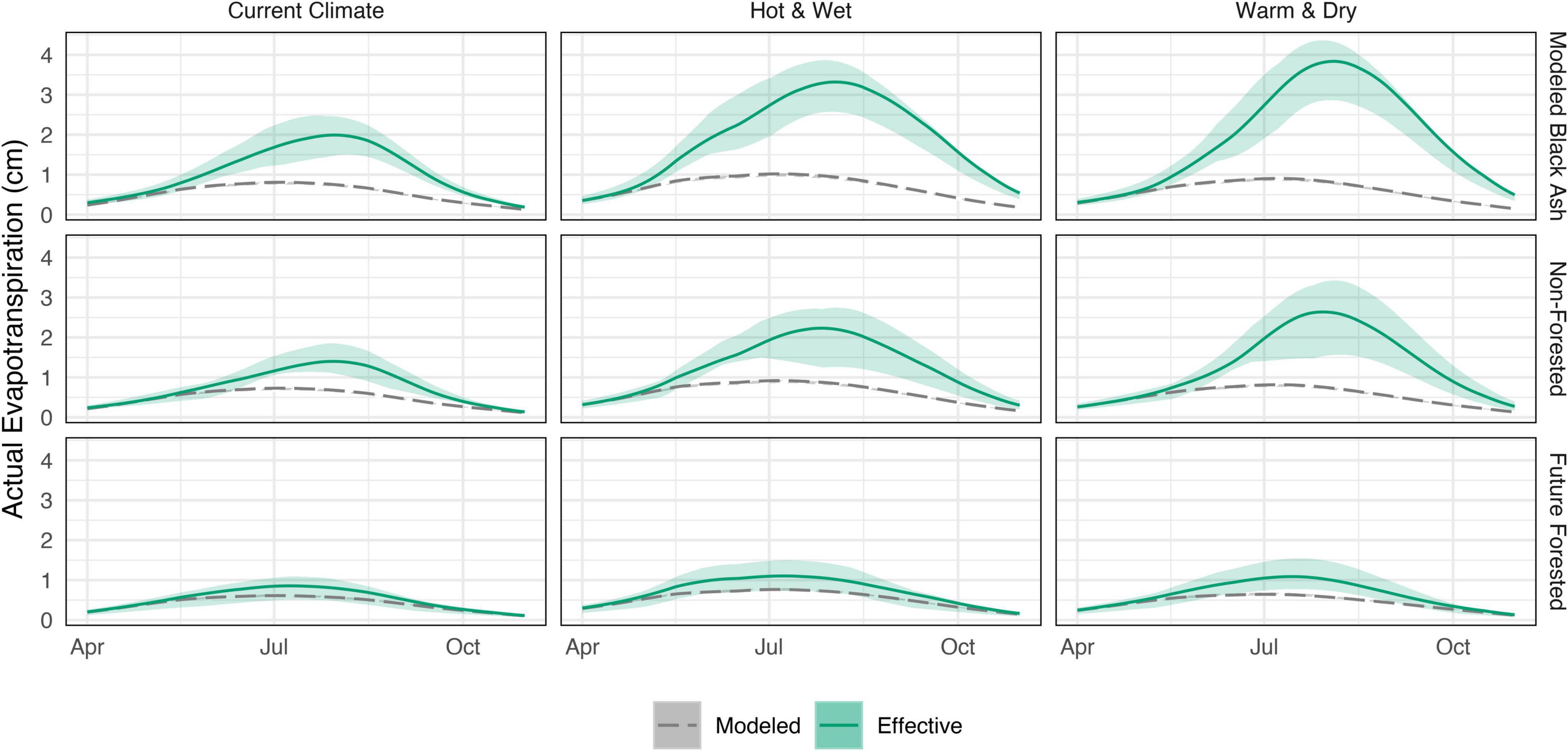
Figure 9. Modeled and effective actual evapotranspiration under various climate scenarios and vegetation conditions. Modeled actual evapotranspiration (AET) is the synthetic potential evapotranspiration (PET) multiplied by the model coefficient used in the relevant wetland model. Effective AET is the modeled AET times the value of ecosystem specific yield (ESy) predicted from the contemporaneous water level, showing the magnitude of water level change. The difference between the two values demonstrates the two-stage impact of reduced ET, where AET and E_Sy are reduced. Effective AET is shown in green with 67% HDCI as a shaded ribbon around the median line. Modeled AET is in gray, but has low variability around daily estimates masking the shaded gray areas.

Reduced evaporation and non-canopy transpiration

We observed wetter conditions under our alternate-forest simulations relative to both black ash and non-forested simulations under all climate scenarios (Figures 5, 7). Two factors are likely contributing to this result. The first is that our alternate-forest composition is known to have lower transpiration rates than the existing black ash canopy (Shannon et al., 2018). As a model choice, we opted to assume that the next most dominant canopy species would be the likely replacement canopy species. The alternate-forest we modeled is a narrow range of potential future forest compositions. Natural regeneration or planting efforts may lead to alternate-forested species composition that more closely matches the evaporative potential of the current black ash canopy. The non-forested conditions used to fit the wetland models consisted of species that shifted in composition toward facultative and obligative wet species (Davis et al., 2017). Secondly, the alternate-forested conditions may have a lower total AET than the non-forested conditions. In black ash wetlands in Minnesota, simulated post-EAB conditions (girdled and standing ash) were found to have higher water levels than sites where the ash stems were harvested and removed (Diamond et al., 2018). The authors attributed the result to reduced solar energy and wind-driven boundary layer mixing due to the still standing stems leading to limited AET. Our conditions have a notable difference from that study in that we are assuming there are living trees on site. However, a closed canopy would have the same effect of reducing open water evaporation and understory transpiration. With sufficiently reduced canopy transpiration the effect of certain forest compositions could result in reduced overall AET.

The contrast between the non-forested and alternate-forested simulated hydrology suggests an important management tool. Iverson et al. (2016) and the work from Looney et al. (2015) and Bolton et al. (2018) laid out a framework and results for evaluating potential replacement species considering site conditions of black ash wetlands. The results presented here show the opportunity for management decisions that consider the impact of future vegetation on site hydrologic conditions. The general trend of drier future conditions can be to some degree counteracted by management for cover with lower evapotranspiration rates. Drier conditions are not always preferable across the landscape and this tactic could be used to retain water on the landscape, creating refugia of standing water or cool moist soils for flora and fauna. Although much of the region is expected to have drier summers, our localized study area is expected to have wetter summers. The impact of climate change in other areas of the region would become even more pronounced because summer precipitation is expected to remain constant or decrease, further increasing the water deficit created by increased evaporative demand. Vegetation conditions would still amplify or counteract climate impacts, and in some areas may become even more important to providing wet or moist refugia on the landscape. Following the EAB-induced loss of black ash, the vegetation conditions of existing black ash-dominated wetlands, as detailed in Looney et al. (2015) and Davis et al. (2017) will likely result in a non-forested (herbaceous or scrub/shrub) or an alternate-forested (comprised of co-dominant canopy species or planted alternatives) wetland. Results presented here suggest that these non-forested wetlands may in fact become even drier than what would result from the influence of the projected drier climate independently, and therefore the expected increased ET may result in a net loss of existing wetland area over time. Whereas, the alternate-forested wetlands are expected to have higher water tables and have wetter site conditions, and these projected wetter conditions may counteract the influence of a drying climate and ultimately result in a lesser net loss of wetland area.

The response of each species and plant community will show individual climate change responses that are not captured in these models and may be non-linear (Short, 2016). Yuan et al. (2019) show that Earth system models participating in the CMIP5 project that vapor pressure deficit (VPD) will continue to increase until 2100, and this projected increase in VPD will likely have negative impacts on vegetation growth in the future as evidenced by the comparison of VPD and normalized differenced vegetation index (NDVI) trends between 1999 and 2015. While the Great Lakes region appears to match the global scale projection of increasing VPD and decreasing NDVI (Yuan et al., 2019), the vegetation response of wetland adapted forested and non-forested species may not be as negatively affected by increasing VPD as is expected in regional- to global-scale upland areas if water levels in the wetlands remain elevated. Based upon the modeled results presented here, the wetter and higher water levels expected in the alternate-forested condition in conjunction with the projected increasing VPD will likely result in greater transpiration (Shannon et al., 2018) but may not necessarily negatively influence forested vegetative growth if a persistent supply of water is available to match the expected increased stomatal conductance. Whereas the drier and lower water tables expected in the non-forested conditions may – similar to the expected regional-scale projections—negatively affect vegetative growth due to limited water supply. Beyond the potential for unforeseen vegetation responses to future climates is the uncertainty of future climate conditions. The authors of the fourth national climate assessment have highlighted that early climate predictions have under-predicted contemporary shifts in response to climate change (Wuebbles et al., 2017). Unfortunately, this statement means that our models built on those simulations may be underestimating the magnitude of future changes and thus our results may be viewed as the lower envelop of potential changes for the region.

Conclusion

Our research has shown that changes in evaporative demand and precipitation regimes will likely result in drier conditions on what are now black ash wetlands. In addition, the functional loss of black ash due to emerald ash borer presents challenges and opportunities for the future of these wetlands. A large extent of forested wetlands may require intervention to retain desired benefits or features they currently provide. These interventions can be used to drive sites toward wetter conditions, retaining water on the landscape that may otherwise be lost under a changing climate.

To implement long-term management objectives in forested wetlands requires a deep understanding of the systems. We have shown that changes in AET can interact with ecosystem specific yield to create feedback loops that may push disturbed black ash wetlands toward new hydrologic steady states. This underscores that knowledge of species adaptation to wet conditions and capacity to respond quickly to drying conditions is critical for projected future site conditions. The transition from black ash to alternative vegetative cover can counteract or amplify the impacts of future conditions with higher evaporative demand. The magnitude of the impact of transition to less inundation-adapted species may be much larger than that of climate change on these systems. Existing results suggesting alternative species should be reevaluated in light of the counteracting effect of climate change on EAB-disturbed black ash wetland hydrology.

Data availability statement

The datasets presented in this study can be found in online repositories. The names of the repository/repositories and accession number(s) can be found at: https://github.com/jpshanno/climate_response.

Author contributions

JS conceived of the experimental and simulation design and led the development and analysis of the wetland model, stochastic weather generator, and simulations. FL and RK provided critical feedback and improvements to the experimental design and manuscript. MV provided critical feedback to the manuscript and analysis and correction of wetland water levels. All authors contributed to the article and approved the submitted version.

Funding

This work was supported by the U.S. Forest Service, Grant/Award Numbers: 17-JV-11 242307-133 and 21-JV-11242307-050, the Graduate School Finishing Fellowship, Michigan Technological University, Michigan Technological University Ecosystem Science Center (ESC), and the USDA National Institute of Food and Agriculture (NIFA) McIntire Stennis Project (Grant Contract Number: NI22MSCFRXXXG027, Proposal: 2109065).

Acknowledgments

JS would like to thank Amy Marcarelli for feedback on this research during his dissertation defense and Andrew Verdin for providing background and example code for stochastic weather generators.

Conflict of interest

The authors declare that the research was conducted in the absence of any commercial or financial relationships that could be construed as a potential conflict of interest.

Publisher’s note

All claims expressed in this article are solely those of the authors and do not necessarily represent those of their affiliated organizations, or those of the publisher, the editors and the reviewers. Any product that may be evaluated in this article, or claim that may be made by its manufacturer, is not guaranteed or endorsed by the publisher.

Supplementary material

The Supplementary Material for this article can be found online at: https://www.frontiersin.org/articles/10.3389/ffgc.2022.957526/full#supplementary-material

Footnotes

1. ^ http://gdo-dcp.ucllnl.org/downscaled_cmip_projections/

References

APHIS (2021). Initial County EAB Detection in North America. Available Online at: http://www.emeraldashborer.info/documents/MultiState_EABpos.pdf [accessed January 4, 2021].

Google Scholar

Arguez, A., Durre, I., Applequist, S., Vose, R. S., Squires, M. F., Yin, X., et al. (2012). NOAA’s 1981 U.S. Climate Normals: an overview. Bull. Am. Meteorol. Soc. 93, 1687–1697. doi: 10.1175/BAMS-D-11-00197.1

PubMed Abstract | CrossRef Full Text | Google Scholar

Baddour, O., and Kontongomde, H. (eds). (2007). The Role of Climatological Normals in a Changing Climate. WCDMP-No. 61, WMO-TD No. 1377. Geneva: World Meteorological Organization.

Google Scholar

Bates, D., Mächler, M., Bolker, B., and Walker, S. (2015). Fitting linear mixed-effects models using lme4. J. Stat. Softw. 67, 1–48. doi: 10.18637/jss.v067.i01

CrossRef Full Text | Google Scholar

Bojanowski, J. S. (2016). Sirad: Functions for Calculating Daily Solar Radiation and Evapotranspiration. Available Online at: https://CRAN.R-project.org/package=sirad

Google Scholar

Bolton, N., Shannon, J., Davis, J., Grinsven, M., Noh, N. J., Schooler, S., et al. (2018). Methods to improve survival and growth of planted alternative species seedlings in black ash ecosystems threatened by emerald ash borer. Forests 9:146. doi: 10.3390/f9030146

CrossRef Full Text | Google Scholar

Brinson, M. M. (1993). A Hydrogeomorphic Classification for Wetlands. Wetlands Research Program Technical Report WRP-DE-4 WRP-DE-4. Vicksburg, MS: US Army Corps of Engineers Waterways Experiment Station. 101.

Google Scholar

Bristow, K. L., and Campbell, G. S. (1984). On the relationship between incoming solar radiation and daily maximum and minimum temperature. Agric. For. Meteorol. 31, 159–166. doi: 10.1016/0168-1923(84)90017-0

CrossRef Full Text | Google Scholar

Burkett, V., and Kusler, J. (2000). Climate change: potential impacts and interactions in wetlands of the United States. J. Am. Water Resour. Assoc. 36, 313–320. doi: 10.1111/j.1752-1688.2000.tb04270.x

CrossRef Full Text | Google Scholar

Bürkner, P.-C. (2017). brms: an R package for bayesian multilevel models using stan. J. Stat. Softw. 80, 1–28. doi: 10.18637/jss.v080.i01

CrossRef Full Text | Google Scholar

Bürkner, P.-C. (2018). Advanced bayesian multilevel modeling with the R package brms. R J. 10, 395–411. doi: 10.32614/RJ-2018-017

CrossRef Full Text | Google Scholar

Byun, K., and Hamlet, A. F. (2018). Projected changes in future climate over the midwest and great lakes region using downscaled Cmip5 Ensembles: projected climate changes over the midwest and great lakes region. Int. J. Climatol. 38, e531–e553. doi: 10.1002/joc.5388

CrossRef Full Text | Google Scholar

Coron, L., Thirel, G., Delaigue, O., Perrin, C., and Andréassian, V. (2017). The suite of lumped gr hydrological models in an R package. Environ. Model. Softw. 94, 166–171. doi: 10.1016/j.envsoft.2017.05.002

CrossRef Full Text | Google Scholar

Davis, J. C., Shannon, J. P., Bolton, N. W., Kolka, R. K., and Pypker, T. G. (2017). Vegetation responses to simulated emerald ash borer infestation in Fraxinus nigra dominated wetlands of Upper Michigan, USA. Can. J. For. Res. 47, 319–330. doi: 10.1139/cjfr-2016-0105

CrossRef Full Text | Google Scholar

Diamond, J. S., McLaughlin, D. L., Slesak, R. A., D’Amato, A. W., and Palik, B. J. (2018). Forested versus herbaceous wetlands: can management mitigate ecohydrologic regime shifts from invasive emerald ash borer? J. Environ. Manag. 222, 436–446. doi: 10.1016/j.jenvman.2018.05.082

PubMed Abstract | CrossRef Full Text | Google Scholar

Gent, P. R., Danabasoglu, G., Donner, L. J., Holland, M. M., Hunke, E. C., Jayne, S. R., et al. (2011). The community climate system model version 4. J. Clim. 24, 4973–4991. doi: 10.1175/2011JCLI4083.1

PubMed Abstract | CrossRef Full Text | Google Scholar

Griffies, S. M., Winton, M., Donner, L. J., Horowitz, L. W., Downes, S. M., Farneti, R., et al. (2011). The GFDL Cm3 coupled climate model: characteristics of the ocean and sea ice simulations. J. Clim. 24, 3520–3544. doi: 10.1175/2011JCLI3964.1

PubMed Abstract | CrossRef Full Text | Google Scholar

Haack, R. A., Jendek, E., Liu, H., Marchant, K. R., Petrice, T. R., Poland, T. M., et al. (2002). The emerald ash borer: a new exotic Pest in North America. Newsl. Mich. Entomol. Soc. 47, 1–5.

Google Scholar

Hargreaves, G. H., and Allen, R. G. (2003). History and evaluation of Hargreaves evapotranspiration equation. J. Irrig. Drain. Eng. 129, 53–63. doi: 10.1061/(ASCE)0733-94372003129:1(53)

CrossRef Full Text | Google Scholar

Hayhoe, K., VanDorn, J., Croley, T., Schlegal, N., and Wuebbles, D. (2010). Regional climate change projections for Chicago and the US great lakes. J. Great Lakes Res. 36, 7–21. doi: 10.1016/j.jglr.2010.03.012

CrossRef Full Text | Google Scholar

Herms, D. A., and McCullough, D. G. (2014). Emerald ash borer invasion of North America: history, biology, ecology, impacts, and management. Annu. Rev. Entomol. 59, 13–30. doi: 10.1146/annurev-ento-011613-162051

PubMed Abstract | CrossRef Full Text | Google Scholar

Horel, J., Splitt, M., Dunn, L., Pechmann, J., White, B., Ciliberti, C., et al. (2002). Mesowest: cooperative mesonets in the Western United States. Bull. Am. Meteorol. Soc. 83, 211–226.

Google Scholar

Hourly Precipitation Data [HPD] (2021). Hourly Precipitation Data [HPD] Network, Version 2.R2. Asheville, NC: NOAA National Centers for Environmental Information.

Google Scholar

Iverson, L., Knight, K. S., Prasad, A., Herms, D. A., Matthews, S., Peters, M., et al. (2016). Potential species replacements for black ash (Fraxinus nigra) at the confluence of two threats: emerald ash borer and a changing climate. Ecosystems 19, 248–270. doi: 10.1007/s10021-015-9929-y

CrossRef Full Text | Google Scholar

Kane, E. S., Veverica, T. J., Tfaily, M. M., Lilleskov, E. A., and Meingast, K. M. (2019). Reduction-oxidation potential and dissolved organic matter composition in northern peat soil: interactive controls of water table position and plant functional groups. J. Geophys. Res. Biogeosci. 124, 3600–3617. doi: 10.1029/2019JG005339

CrossRef Full Text | Google Scholar

Kolka, R., D’Amato, A., Wagenbrenner, J., Slesak, R., Pypker, T., Youngquist, M., et al. (2018). Review of ecosystem level impacts of emerald ash borer on black ash wetlands: what does the future hold? Forests 9:179. doi: 10.3390/f9040179

CrossRef Full Text | Google Scholar

Krause, P., Boyle, D. P., and Bäse, F. (2005). Comparison of different efficiency criteria for hydrological model assessment. Adv. Geosci. 5, 89–97. doi: 10.5194/adgeo-5-89-2005

CrossRef Full Text | Google Scholar

Lenth, R. V. (2021). Emmeans: Estimated Marginal Means, Aka Least-Squares Means. Available Online at: https://github.com/rvlenth/emmeans

Google Scholar

Loheide, S. P. (2008). A method for estimating subdaily evapotranspiration of shallow groundwater using diurnal water table fluctuations. Ecohydrology 1, 59–66. doi: 10.1002/eco.7

CrossRef Full Text | Google Scholar

Looney, C. E., D’Amato, A. W., Fraver, S., Palik, B. J., and Reinikainen, M. R. (2016). Examining the influences of tree-to-tree competition and climate on size-growth relationships in hydric, multi-aged Fraxinus nigra stands. For. Ecol. Manag. 375, 238–248. doi: 10.1016/j.foreco.2016.05.050

CrossRef Full Text | Google Scholar

Looney, C. E., D’Amato, A. W., Palik, B. J., and Slesak, R. A. (2015). Overstory treatment and planting season affect survival of replacement tree species in emerald ash borer threatened Fraxinus nigra forests in Minnesota, USA. Can. J. For. Res. 45, 1728–1738. doi: 10.1139/cjfr-2015-0129

CrossRef Full Text | Google Scholar

Looney, C. E., D’Amato, A. W., Palik, B. J., Slesak, R. A., and Slater, M. A. (2017). The response of Fraxinus nigra forest ground-layer vegetation to emulated emerald ash borer mortality and management strategies in Northern Minnesota, USA. For. Ecol. Manag. 389, 352–363. doi: 10.1016/j.foreco.2016.12.028

CrossRef Full Text | Google Scholar

McElreath, R. (2020). Statistical Rethinking: A Bayesian Course with Examples in r and Stan, 2nd Edn. Boca Raton, FL: Chapman & Hall/CRC.

Google Scholar

McLaughlin, D. L., and Cohen, M. J. (2014). Ecosystem specific yield for estimating evapotranspiration and groundwater exchange from diel surface water variation: ecosystem s y for estimating et and groundwater exchange. Hydrol. Process. 28, 1495–1506. doi: 10.1002/hyp.9672

CrossRef Full Text | Google Scholar

McLaughlin, D. L., Diamond, J. S., Quintero, C., Heffernan, J., and Cohen, M. J. (2019). Wetland connectivity thresholds and flow dynamics from stage measurements. Water Resour. Res. 55, 6018–6032. doi: 10.1029/2018WR024652

CrossRef Full Text | Google Scholar

Menne, M. J. I, Durre, B., Korzeniewski, S., McNeal, K., Thomas, X., Yin, S., et al. (2012a). Global Historical Climatology Network - Daily (GHCN-Daily), Version 3.28-Upd-2021031419. Asheville, NC: NOAA National Centers for Environmental Information.

Google Scholar

Menne, M. J., Durre, I., Vose, R. S., Gleason, B. E., and Houston, T. G. (2012b). An overview of the global historical climatology network-daily database. J. Atmos. Ocean. Technol. 29, 897–910. doi: 10.1175/JTECH-D-11-00103.1

PubMed Abstract | CrossRef Full Text | Google Scholar

Moomaw, W. R., Chmura, G. L., Davies, G. T., Finlayson, C. M., Middleton, B. A., Natali, S. M., et al. (2018). Wetlands in a changing climate: science, policy and management. Wetlands 38, 183–205. doi: 10.1007/s13157-018-1023-8

CrossRef Full Text | Google Scholar

Moriasi, D. N., Gitau, M. W., Pai, N., and Duggaupati, P. (2015). Hydrologic and water quality models: performance measures and evaluation criteria. Trans. ASABE 58, 1763–1785. doi: 10.13031/trans.58.10715

CrossRef Full Text | Google Scholar

Notaro, M., Bennington, V., and Vavrus, S. (2015). Dynamically downscaled projections of lake-effect snow in the great lakes basin. J. Clim. 28, 1661–1684. doi: 10.1175/JCLI-D-14-00467.1

PubMed Abstract | CrossRef Full Text | Google Scholar

Osborn, H. B., Renard, K. G., and Simanton, J. R. (1979). Dense networks to measure convective rainfall in the Southwestern United States. Water Resour. Res. 15, 1701–1711.

Google Scholar

Pierce, D. W., Cayan, D. R., and Thrasher, B. L. (2014). Statistical downscaling using localized constructed analogs (LOCA). J. Hydrometeorol. 15, 2558–2585. doi: 10.1175/JHM-D-14-0082.1

PubMed Abstract | CrossRef Full Text | Google Scholar

R Core Team (2019). R: A Language and Environment for Statistical Computing. Vienna: R Foundation for Statistical Computing.

Google Scholar

Richardson, C. W. (1981). Stochastic simulation of daily precipitation, temperature, and solar radiation. Water Resour. Res. 17, 182–190. doi: 10.1029/WR017i001p00182

CrossRef Full Text | Google Scholar

Rood, R., and Briley, L. (2018). Great Lakes Ensemble April 2017 - April 2018 Progress Report. Ann Arbor, MI: Great Lakes Integrated Sciences + Assessments.

Google Scholar

Scheffer, M., and Carpenter, S. R. (2003). Catastrophic regime shifts in ecosystems: linking theory to observation. Trends Ecol. Evol. 18, 648–656. doi: 10.1016/j.tree.2003.09.002

CrossRef Full Text | Google Scholar

Shannon, J., Liu, F., Van Grinsven, M., Kolka, R., and Pypker, T. (2022). Magnitude, consequences, and correction of temperature-derived errors for absolute pressure transducers under common monitoring scenarios. Hydrol. Process. 36, e14457. doi: 10.1002/hyp.14457

CrossRef Full Text | Google Scholar

Shannon, J., Van Grinsven, M., Davis, J., Bolton, N., Noh, N. J., Pypker, T., et al. (2018). Water level controls on sap flux of canopy species in black ash wetlands. Forests 9:147. doi: 10.3390/f9030147

CrossRef Full Text | Google Scholar

Short, F. T. (2016). Impacts of climate change on submerged and emergent wetland plants. Aquat. Bot. 135, 3–17. doi: 10.1016/j.scitotenv.2018.06.080

PubMed Abstract | CrossRef Full Text | Google Scholar

Slesak, R. A., Lenhart, C. F., Brooks, K. N., D’Amato, A. W., and Palik, B. J. (2014). Water table response to harvesting and simulated emerald ash borer mortality in black ash wetlands in Minnesota, USA. Can. J. For. Res. 44, 961–968. doi: 10.1139/cjfr-2014-0111

CrossRef Full Text | Google Scholar

Soylu, M. E., Lenters, J. D., Istanbulluoglu, E., and Loheide, S. P. (2012). On evapotranspiration and shallow groundwater fluctuations: a Fourier-based improvement to the White method. Water Resour. Res. 48:W06506. doi: 10.1029/2011WR010964

CrossRef Full Text | Google Scholar

Stan Development Team (2022). Stan Modeling Language Users Guide and Reference Manual, 2.29. Available Online at: https://mc-stan.org

Google Scholar

Swanston, C. W., Janowiak, M. K., Brandt, L. A., Butler, P. R., Handler, S. D., Shannon, P. D., et al. (2016). Forest Adaptation Resources: Climate Change Tools and Approaches for Land Managers, 2nd Edn. Newtown Square, PA: U.S. Department of Agriculture.

Google Scholar

Valéry, A., Andréassian, V., and Perrin, C. (2014). ‘As simple as possible but not simpler’: what is useful in a temperature-based snow-accounting routine? Part 1 comparison of six snow accounting routines on 380 catchments. J. Hydrol. 517, 1166–1175. doi: 10.1016/j.jhydrol.2014.04.059

CrossRef Full Text | Google Scholar

Van Grinsven, M. J., Shannon, J. P., Davis, J. C., Bolton, N. W., Wagenbrenner, J. W., Kolka, R. K., et al. (2017). Source water contributions and hydrologic responses to simulated emerald ash borer infestations in depressional black ash wetlands. Ecohydrology 10:e1862. doi: 10.1002/eco.1862

CrossRef Full Text | Google Scholar

van Vuuren, D. P., Edmonds, J., Kainuma, M., Riahi, K., Thomson, A., Hibbard, K., et al. (2011). The representative concentration pathways: an overview. Clim. Change 109, 5–31. doi: 10.1007/s10584-011-0148-z

CrossRef Full Text | Google Scholar

Verdin, A., Rajagopalan, B., Kleiber, W., and Katz, R. W. (2015). Coupled stochastic weather generation using spatial and generalized linear models. Stoch. Environ. Res. Risk Assess. 29, 347–356. doi: 10.1007/s00477-014-0911-6

CrossRef Full Text | Google Scholar

Watras, C. J., Morrison, K. A., Rubsam, J. L., and Buffam, I. (2017). Estimates of evapotranspiration from contrasting Wisconsin peatlands based on diel water table oscillations. Ecohydrology 10:e1834. doi: 10.1002/eco.1834

CrossRef Full Text | Google Scholar

White, W. N. (1932). A Method of Estimating Ground-Water Supplies Based on Discharge by Plants and Evaporation from Soil: Results of Investigations in Escalante Valley, Utah, Vol. 659. Washington, DC: U.S. Government Printing Office.

Google Scholar

Wilks, D. S. (2012). Stochastic weather generators for climate-change downscaling, part II: multivariable and spatially coherent multisite downscaling: stochastic weather generators for climate-change downscaling. Wiley Interdiscip. Rev. Clim. Change 3, 267–278. doi: 10.1002/wcc.167

CrossRef Full Text | Google Scholar

Wilks, D. S., and Wilby, R. L. (1999). The weather generation game: a review of stochastic weather models. Prog. Phys. Geogr. 23, 329–357. doi: 10.1177/030913339902300302

CrossRef Full Text | Google Scholar

Wuebbles, D. J., Fahey, D. W., and Hibbard, K. A. (2017). Climate Science Special Report: Fourth National Climate Assessment, Vol. I., Washington, DC: U.S. Global Change Research Program.

Google Scholar

Yuan, W., Zheng, Y., Piao, S., Ciais, P., Lombardozzi, D., Wang, Y., et al. (2019). Increased atmospheric vapor pressure deficit reduces global vegetation growth. Sci. Adv. 5:eaax1396. doi: 10.1126/sciadv.aax1396

PubMed Abstract | CrossRef Full Text | Google Scholar

Zhu, J., Young, M., Healey, J., Jasoni, R., and Osterberg, J. (2011). Interference of river level changes on riparian zone evapotranspiration estimates from diurnal groundwater level fluctuations. J. Hydrol. 403, 381–389. doi: 10.1016/j.jhydrol.2011.04.016

CrossRef Full Text | Google Scholar