Using essential biodiversity variables to assess forest ecosystem integrity

1. Introduction

Forests are complex ecosystems, and their physical, biological, and functional components interact with each other (Hansen et al., 2021), which is fundamental to maintaining ecosystem resilience and the capacity to provide ecosystem services (Watson et al., 2018). However, anthropogenic drivers such as land-use change threaten forests and exacerbate climate change and biodiversity loss (Díaz et al., 2019). Additionally, biodiversity loss may not be effectively reverted, focusing only on forest cover loss without considering other components of ecosystem functioning. For instance, fragmentation may lead to reduced habitat for animal species and significant degradation of the forest ecosystem (Morris, 2010), resulting in reduced functioning of the systems on which humans and other organisms depend (Grantham et al., 2020). Therefore, projects related to climate mitigation and biodiversity loss focus not only on one specific ecosystem service but also include the components of ecosystem integrity to deliver long-term benefits for people and the environment.

The protection of forests and the assessment and monitoring of ecosystem integrity across scales are some of the key targets of international frameworks such as the Post-2020 Global Biodiversity Framework and the United Nations 2030 Agenda (CBD/SBSTTA/24/3/Add.2, 2021). Ecosystem integrity has been defined as “a measure of ecosystem structure, function and composition relative to the reference state of these components being predominantly determined by the extant climatic–geophysical environment” (Hansen et al., 2021). It describes how complete, healthy, and resilient an ecosystem is to both natural and human perturbations (Seddon et al., 2021). The structure of the forest encompasses the three-dimensional architecture of individual plants and the connection of their attributes (Hansen et al., 2021), while the function characterizes the movement or storage of energy or matter within an ecosystem (Bellwood et al., 2019). The composition describes how a forest’s natural features are distributed within the ecosystem (genetic diversity, species richness, and community assemblages).

In recent decades the number of open-source satellite image collections has increased tremendously, which resulted in a growing number of high-quality biological remote-sensing products (de Paula et al., 2019). One well-known example is the Global Forest Cover Change map by Hansen et al. (2013). These remote sensing products are also known as Earth Observations (EO) and are particularly useful due to their global coverage and high temporal resolution (Skidmore and Pettorelli, 2015). The potential of EOs to measure and monitor biological products globally has not gone unnoticed. In 2013, the Group on Earth Observations Biodiversity Observation Network (GEO BON) set up a new framework to develop Essential Biodiversity Variables (EBVs) (Pereira et al., 2013). EBVs can be a combination of in-situ and remotely sensed data, or they can be derived from either (Giuliani et al., 2017; Schmeller et al., 2017; Kissling et al., 2018). There are currently 20 EBVs in six classes, including genetic composition, species populations, species traits, community composition, ecosystem function and structure (Hansen et al., 2021). Since the introduction of this concept, global political frameworks have proposed EBVs as the basis for monitoring advancements towards biological targets (Geijzendorffer et al., 2016). However, researchers have emphasized the importance of continuous testing of the application of EBVs across different scales and ecosystems (Pereira et al., 2013).

Reliable and consistent monitoring of forest ecosystem integrity is crucial to mitigating climate change and biodiversity loss (Keenan et al., 2015). Integrating different EBVs to monitor ecosystems globally may enable the development of a more consistent, accurate and scalable framework for sustainable management and global collaboration (Reddy, 2021). Although scientists have attempted to quantify ecosystem integrity, few studies have explored how EBVs can be organized in an effective workflow to create a composite index describing forest ecosystem integrity and differentiate between plots at the local and global scale (Hansen et al., 2021). Here, we build on previous studies defining forest ecosystem integrity by using available EBVs to present and test a framework which assesses forest ecosystem integrity of plots at the global scale. Using readily available EBVs to assess and monitor ecosystem integrity will help scientists and policymakers to acquire comparable information more easily on the state of ecosystems. Ultimately, knowing where ecosystem integrity is high or low may also help land managers and conservationists prioritize areas of high importance.

2. Materials and methods

2.1. Measuring ecosystem integrity

To assess forest ecosystem integrity, we developed an Ecosystem Integrity Index score (EII_score) for forested plots based on the aggregation of spatially explicit EBVs representing structure, function, and composition, the three components defining ecological integrity. Our framework is consistent with previous definitions of ecosystem integrity, such as the one provided by Hansen et al. (2021). We focused on forested ecosystems across the globe (Hansen et al., 2013), as EBVs of forested ecosystems are the most readily available compared to other ecosystems.

The first component of ecosystem integrity, structure, is designed to capture aspects of ecosystems related to vegetation structure and spatial configuration, including fragmentation. The second component, function, captures the amount of specific ecosystem function variables such as energy flow and nutrient cycling. The third component captures ecosystem composition, which accounts for species abundance and community composition.

Here we used the following indicators to characterize the elements of ecosystem integrity: the Biodiversity Intactness Index (BII, Newbold et al., 2016) representing the element composition, Net Primary Productivity (NPP, Running and Zhao, 2019) describing the element function, and Loss in Forest Connectivity (LFC, Grantham et al., 2020) representing the element structure (Table 1). Each EBV was selected according the following criteria: ability to describe of the ecosystem integrity components, resolution, open access and publication date.

TABLE 1

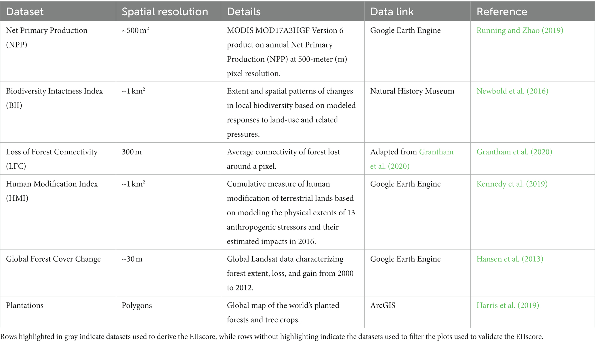
Table 1. Datasets used to calculate the EII_score with their respective resolution, a brief description of what the data entails and the reference.

The BII is defined as the average richness- and area-weighted impact of a set of activities on the populations of a given group of organisms in a specific area (Scholes and Biggs, 2005; Newbold et al., 2016) based on the Projecting Responses of Ecological Diversity In Changing Terrestrial Systems (PREDICTS) database (Hudson et al., 2017) with the most recent update occurring in October 2021 (Phillips et al., 2021). Newbold et al. (2016) developed hierarchical mixed-effects models that considered four human-pressure variables, including land use, land-use intensity, human population density and distance to the nearest road to explain differences in local biodiversity among sites. Biodiversity is measured as sampled species richness and abundance based on the PREDICTS database. Further details are provided in Newbold et al. (2016). The resolution of the BII is 1 km².

NPP is a well-known representation of the net input of carbon to vegetation impacted inter-alia by climate (e.g., solar inputs, precipitation), soil quality, and nutrient status (Walker et al., 2021), with a well-known relationship to biomass production (Vicca et al., 2012) and carbon-use efficiency (DeLucia et al., 2007).

LFC represents the average connectivity of a forest around a pixel and was estimated following Grantham et al. (2020). The method compares currently observed forest extent with potential forest extent given human modification to the landscape to ensure that areas with naturally low connectivity are not penalized. The final estimate ranges from 0 to 1, so low values represent the least loss and high values represent the greatest loss.

As both NPP and LFC have different resolutions (1 km²) from the BII, we used a bilinear method (Gorelick et al., 2017) to resample the pixel size of NPP and LFC to 1 km². This step was necessary to enable us to perform zonal statistics and derive the EII. Our EII has therefore a pixel size of 1 km².

The EII_score of any given forested land can be calculated using three EBVs, e.g., BII, NPP and LFC. First, (i) we calculate the global 90th percentile values for each of the three EBVs considering only the global intact forest area (Hansen et al., 2013) that has a Global Human Footprint Index value (Kennedy et al., 2019) of less than 0.4 and which is outside plantations mapped by Harris et al. (2019). Then, (ii) for each pixel, we calculate the relative value of each EBV by dividing the pixel value by the corresponding global 90th percentile value (Figure 1), with pixels with value above 90th percentile were given the value of 1. Subsequently, (iii) we calculate the EII value for each pixel in the study forest plots by taking the mean of the relative BII, NPP and LFC values. Note, using this methodology, EII values should only be calculated for forested areas where the BII, NPP and LFC values are known. Finally, (iv) the EII_score of the plot is found by taking the sum of all EII pixels in that given plot (Figure 1). Throughout this paper, we use two different notations: EII and EII_score. With EII, we refer to the index at the pixel level and with EII_score to the index at the plot level.

FIGURE 1

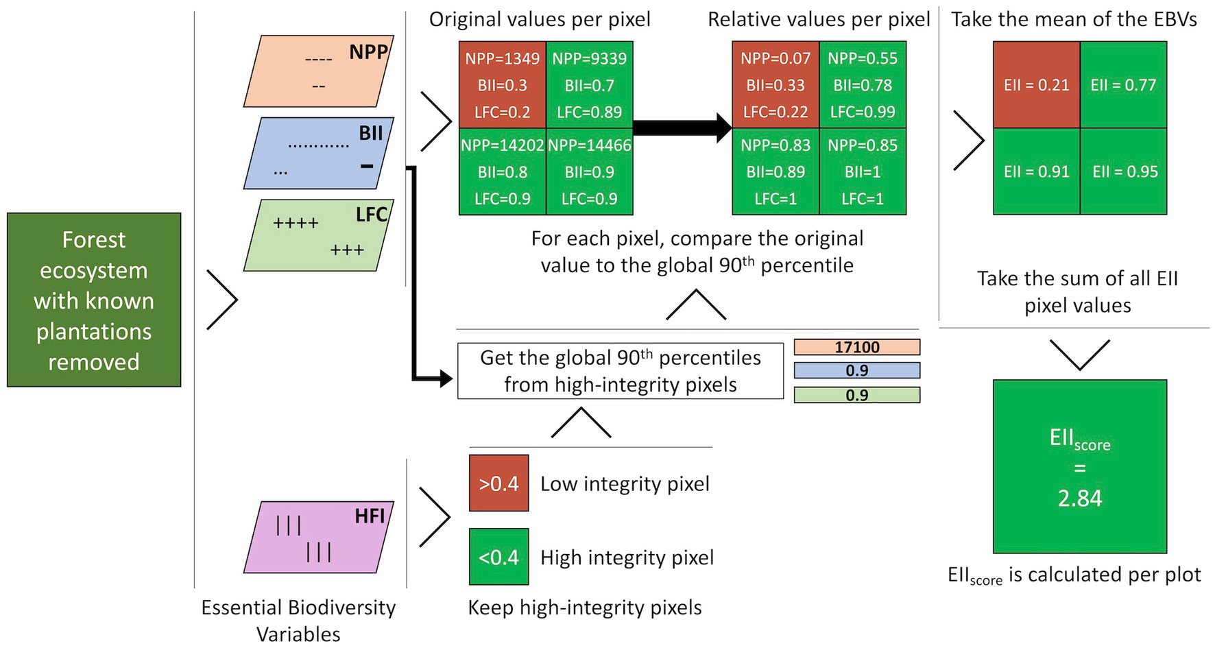
Figure 1. Visual representation of the workflow used to calculate the EII_score for forested plots. NPP is the Net Primary Product, BII is the Biodiversity Intactness Index, LFC is the Loss of Forest Connectivity, and HFI is the Human Footprint Index. EII is the ecosystem integrity index. The EIIscore, NPP, BII, LFC, and HFI all have a pixel size of 1 km². Note values shown are for this example only and are not real values from the sampled lands in this study.

2.2. Extracting validation plots

To validate the EII_score, we first extracted 333 plots (polygons) of 5 km² through stratified sampling. We hypothesized that different forest conditions could affect ecosystem integrity (Potapov et al., 2011). The plots were selected in two categories; 166 plots were assigned the “Top” category with high-quality forests, and 167 lower-quality forests were assigned the “Down” category. The high-quality forest plots were selected so that they would contain forest cover classified with no forest conversion or degradation by Potapov et al. (2011), while lower-quality forest plots were selected to have forests classified by Potapov et al. (2011) that have not experienced loss and have at least 30% forest cover by Hansen et al. (2013), however, are classified as deforested or partially deforested by Potapov et al. (2011).

All plots were extracted outside of plantations (Harris et al., 2019), protected areas (UNEP-WCMC and IUCN, 2022) and islands (Sayre et al., 2019), were located below 1,000 m altitude (Sayre et al., 2019) and not located in Antarctica. Each plot was extracted by hand through Google Earth Engine, was automatically assessed for suitability and manually assessed through visual confirmation (Supplementary Figure 1). Suitability was acknowledged when more than 90% of the plot was covered with intact forest (Hansen et al., 2013).

For each of the plots, the mean biomass density according to Global Ecosystem Dynamics Investigation (GEDI) L4B product (Dubayah et al., 2022) and the mean canopy height (Potapov et al., 2021) were recorded to compare the relationship between the EII_score and these variables.

2.3. Statistical analyses

Using the 333 plots mentioned above, we tested for significant differences between areas of high integrity (“Top”) and low integrity (“Down”). After testing for normality of the data through a Shapiro–Wilk test and visual assessment of the Q-Q plots and histograms, we determined that the data were non-normally distributed, despite transformations and removal of outliers. Thus, we moved on with a nonparametric Kruskal Wallis test using R (package stats v4.1.1) to test if the response variable (EII_score) could be explained by the explanatory variable (Categories: ‘Top’, ‘Down’).

2.4. Sensitivity and validation analyses

We performed a sensitivity analysis to assess to what extent the results for the EII_score are sensitive to the weight used to define the importance of the different indicators making up the EII. To assess the sensitivity of EII_score to weight, we compared the degree of concordance between plot ranking estimated by the EII_score considering BII, NPP and LFC having the same weight to the median plot ranking estimated by considering the following weight possibilities: BII has weight 0, BII has weight ½, LFC has weight 0, LFC has weight ½, NPP has weight 0, and NPP has weight ½. The benefit of the EII_score is that it provides a single and simple measure that can be used to monitor progress and inform management planning without having to measure the full array of metrics related to forest integrity. Such benefit of an ecosystem integrity composite index and exercise of validation considering the correlation with other metrics has been previously used for other ecosystem integrity indices, such as the forest landscape integrity index (Duncanson et al., 2022). Here, we present an example of a validation exercise demonstrating how EII_score is correlated with field measurements related to forest conditions, specifically canopy height and biomass. All these analyses were done considering each of our 333 plots.

Using a Kendall Tau correlation test (R package stats v4.1.1), we estimated if there was a significant correlation between our EII_score and the validation datasets of biomass and canopy height. All data were tested for normality with a Shapiro–Wilk test (R package stats v4.1.1). A visual analysis of the residual distribution was done before moving on to a parametric or non-parametric test.

We also validated our EII against the forest landscape integrity index from Grantham et al. (2020), which is a well-validated index of forest modification, and therefore, forest integrity. We extracted the average values of our index (EII) and the average values of the forest landscape integrity index (FLII) from Grantham et al. (2020) by forested biomes. We extracted only values of both indices that overlapped with the map of intact forest landscapes (Potapov et al., 2017). With this analysis, we provide a better representation of our index across biomes. As our EII includes an indicator, the LFC, which is also included in the FLII, we performed a sensitivity analysis to prevent a potential similarity between EII and FLII due to the influence of LFC. We calculated global maps of the EII considering the absolute relative change for each indicator (BII, LFC, and NPP), highlighting which has the lowest deviation from the EII at every geographical point. This approach captures the magnitude of deviation without bias towards its direction. By analyzing the geographical distribution of these deviations, we can discern if a particular indicator consistently dominates or if the influence is balanced among all three.

3. Results

Model results from our plots (n = 333) revealed that the EII_score strongly related to the categories of forest condition (Down: n = 167, Top: n = 166). Furthermore, the EII_score was not sensitive to weight but was sensitive to plot size. Forest condition metrics, including biomass and canopy height, were correlated with the EII_score. Forests with high ecosystem integrity are located particularly in the Boreal forests and in the tropical rain forests in South America, Africa and Asia (Figure 2).

FIGURE 2

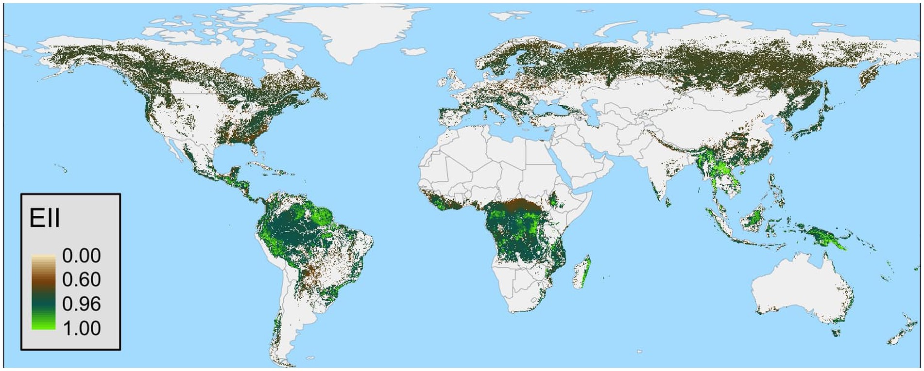
Figure 2. Global map of the ecosystem integrity index. The map is not in the original resolution of 1km² for representation proposal.

3.1. Assessment of ecosystem integrity index

Our results showed a significant difference between EII_score in the forest condition categories ‘Top’ and ‘Down’ (χ2 = 19.193, df = 1, p < 0.001). We found that Top category has significantly higher values of the EII_score, with a mean of 5.88 (CI: 5.53–6.23), whereas the Down category has a mean of 4.97 (CI: 4.67–5.26) (Figure 3).

FIGURE 3

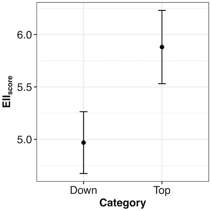
Figure 3. Mean (± 95% confidence intervals) of the EII_score for the 227 plots by forest condition category type (levels: Down, Top). A lower EII_score indicates that the structure, function, and composition were lower, whereas a higher EII_score means those predictors were higher. Confidence intervals are of similar size. EII is the ecosystem integrity index.

3.2. Assessment of sensitivity and validation

We used the Kendall concordance coefficient to verify if the median rank of all plots across the six different weight possibilities (y-axis in Figures 4A,B) changed, considering the situation where all indicators have the same weight (EII_score reference weight x-axis in Figures 4A,B). Considering Top category, we did not find a significant change in the rank of the plots when using different weights for the indicators (Kendall coefficient = 0.93, P ~ 0). Similarly, we did not find a significant change in the rank of the plots when using different weights for the indicators considering the Down category (Kendall coefficient = 0.92, P ~ 0) (Figure 4).

FIGURE 4

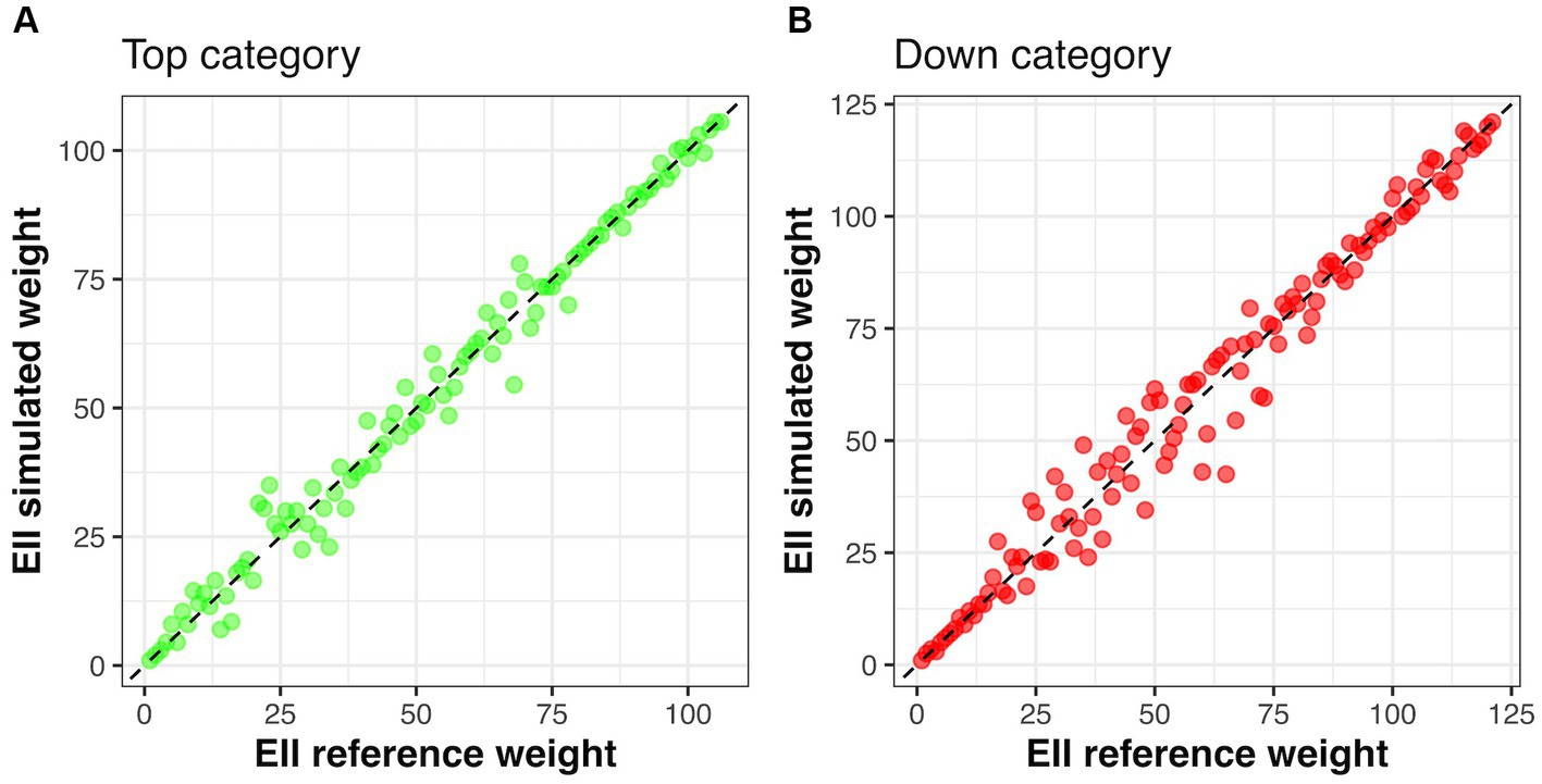
Figure 4. The relationship among the median rank of each plot with a given category compared to the reference estimation of EII_score where the three indicators have the same value. (A) shows the relationship considering plots within the category top and (B) plots within the category down. Note that most points in both figures align with a 1:1 dashed line, which indicates that plots did not change their original rank (EII_score reference weight – all indicators have the same weight) in relation to the median across a plot rank considering six possibilities of weights (EII_score simulated rank) as explained in the text. EII is the ecosystem integrity index.

Metrics related to field measurements of forest conditions, like biomass and canopy height, can be described by the EII_score in the 333 plots. The positive term of biomass (z = 2.859, p = 0.004) and the Kendall concordance coefficient (τ = 0.194) illustrate the weak but significant correlation with the EII_score (Figure 5A). Confidence intervals around the trend are smaller in areas with lower biomass; thus, the EII_score is more likely to give accurate results in areas with biomass up to 200 Mg ha⁻¹. Canopy height, like biomass, was positively correlated (z = 3.610, p < 0.001) with the EII_score in the plots and the Kendall concordance coefficient (τ = 0.245) showed a weak correlation, too (Figure 5B). The confidence intervals around the trend for the EII_score compared to canopy height are relatively small, particularly between the 10–20 m height range.

FIGURE 5

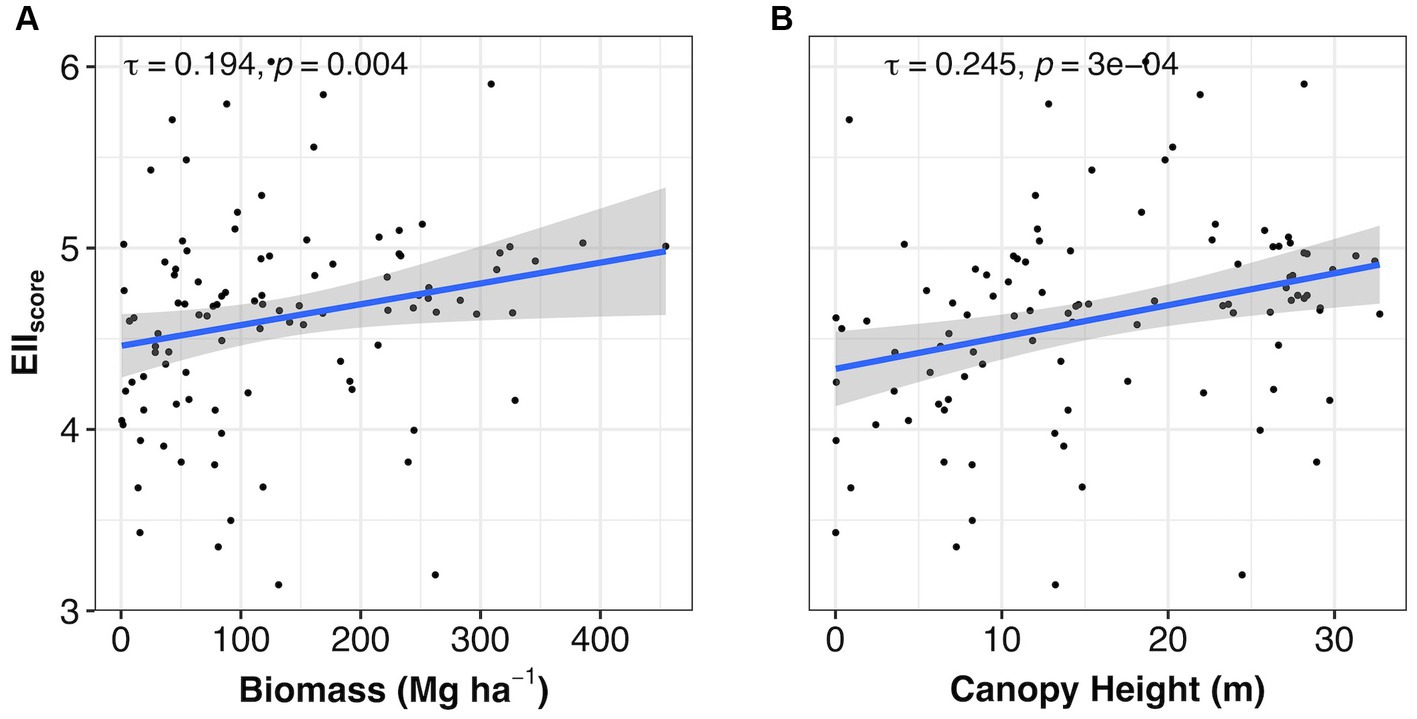
Figure 5. Relationship of the EII_score with (A) biomass and (B) canopy height for the 227 plots. The raw values (as jitter) and the effects with their respective confidence intervals (95%) are shown. Additionally, the Kendall Tau coefficient and the respective value of p are given. A lower EII_score indicates the structure, function and composition were lower, whereas a higher EII_score means those predictors were higher. EII is the ecosystem integrity index.

We found a strong agreement between the average values of our EII across forested biomes with the FLII (Figure 6). Our results also confirmed that the concordance between the EII and the LFII is not driven by any single indicator (Supplementary Figure S4).

FIGURE 6

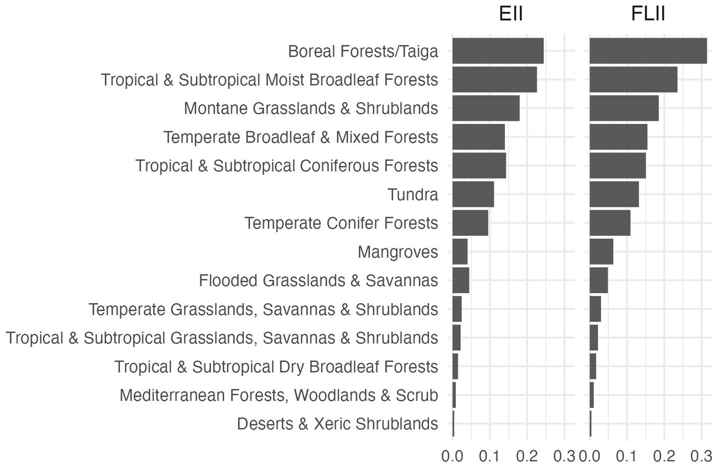
Figure 6. Average values of the ecosystem integrity index (EII) and the forest landscape integrity index (FLII) from Grantham et al. (2020). Note that the average values per biome are almost the same for both indices.

3.3. Uncertainty

The individual components of the EII_score (i.e., BII, NPP, and LFC) all contain inherent uncertainty and variability derived from measurement errors associated with spatial and temporal scales across datasets. In addition, each of the underlying components were developed for other purposes. Thus, qualitative uncertainty is also associated with combining and applying these individual components in different contexts and answering different questions. Underlying uncertainties associated with each individual component apply equally to the EII_score.

The 333 plots were assessed for differences between the “Top” and “Down” classifications. A significant difference between the two categories was apparent but came with inherent uncertainty. Confidence intervals for the EII_score, which were developed graphically using the R package ggplot2 (v. 3.3.6), represent the confidence that the total sum of EII_score values of all the pixels in a “Top” or “Down” category land falls within a certain range. The results showed us that there was a 95 percent chance that our output was correct and that the EII_score was significantly different in the “Top” category compared to the “Down” category. Despite this certainty, the underlying variables increased the uncertainty of our results.

The primary uncertainty associated with the BII is that the species population sampling is not comprehensive. In practical terms, species may or may not be observed at any given sampling location for reasons other than that they were not actually present. Related to species absence/presence is species misidentification. Another uncertainty is that the data in the PREDICTS database (Hudson et al., 2017) are for individual species and, by definition, do not address the impacts of human activities on species interactions or the importance of trophic relationships. Finally, these data are designed to be used in localized contexts, while the EII_score is used to make global-level inferences.

The loss in forest connectivity is calculated as the ratio between the current forest configuration around each pixel to the potential forest configuration (Grantham et al., 2020). As the current forest configuration is represented by the forest cover maps from Hansen et al. (2013), likely, uncertainties associated with the estimation of forest cover maps (e.g., cloud cover, edge effects, changing land use at differing spatial and temporal scales) are introduced when estimating the loss in forest connectivity.

4. Discussion

The EII_score provides an indication of how forest ecosystems across the world perform, considering ecological integrity. Our index is built on the efforts to operationalize the concept of ecosystem integrity across scales using satellite-based EOs and essential EBVs (Hansen et al., 2021). However, our approach differs from previous studies as we not only produced a global map of EII_score, but we also developed a scalable workflow that estimates EII_score at local scales but can easily be applied at larger scales. Our index showed an important property: it is insensitive to the weight used for the indicators of ecosystem integrity (structure, function, and composition). Overall, our results suggest that our index provides a reliable picture of the plots’ performance that is not driven by the importance (weight) assigned to the EII_score indicators. However, it can be used to identify the importance of area-based conservation efforts. Both characteristics are important in the context of ongoing efforts to support the monitoring and reporting of progress within the Post-2020 Global Biodiversity Framework.

The EII_score differentiated pristine from degraded forests globally, indicating that the combination of EBVs used in this study can capture different aspects of ecosystem integrity. Previous studies have emphasized the need to reconnect forested habitats to protect threatened species (e.g., Newmark et al., 2017) and thus highlight the need for an index that can measure and monitor multiple interdependent ecosystem characteristics. This study focused on differences in ecosystem integrity among plots on the global scale. Based on such an assessment, policymakers and institutions facilitating monetary incentives to conserve forested lands can make key policy decisions related to the conservation of ecosystems. However, we recognize that measuring the EII_score at other scales (e.g., global, biome, political region, ecoregion) is fundamental to halting forest integrity reduction (Keenan et al., 2015). For example, local forest management strategies will need to calculate the EII_score over much smaller scales to facilitate comparisons across forests with similar characteristics. Our EII_score has a resolution of 1 km², which is why we recommend using the EII_score only over large, forested areas to increase the variety of pixels. Additionally, this coarse resolution has resulted in some regions being assigned forest pixels even though no forest exists. This results from edge effects, which occur on the edges of plots. Edge effects are a result of pixels being square and the size of their resolution. Pixels can not be split or cut off, so sometimes the edge of a pixel falls inside or outside a plot of interest. In this example, some areas have forests, but on the edge of the forests, there is some overlap of forest pixels into areas without forests. When more detailed EBVs regarding biodiversity become available, we will be able to improve the quality of the resolution and thus reduce the edge effects.

Weights may have an impact on the value of a composite index, as weighting is strongly related to how the information conveyed by the different dimensions is aggregated into a composite index. Here we used only one indicator to represent each of the components of ecosystem integrity and considered our main underlying objective that each indicator has the same importance to ecosystem integrity. Indeed, we did not find a significant difference between the median EII_score using equal weight compared to the six possibilities of assigning different weights to the EII_score indicators. It is likely that we could have found a different result if we had used more indicators that are interrelated or if we had used more possibilities of weight distribution among the indicators than the six we used here. Note that when one indicator has weight 0, the other two indicators have weight ½, and when one indicator has weight ½, the other two indicators have weight ¼. Additionally, we tested for linearity of the EII_score with plot size (Supplementary Methods). Finally, we acknowledge that the EII_score may correlate with a broad range of metrics related to forest integrity and anthropogenic pressures. Examples of these metrics include measures related to forest condition (e.g., canopy height, biomass, structural complexity), forest ecosystem state (e.g., species diversity and abundance), and the intensity of anthropogenic pressures (e.g., land conversion). However, independently of the method used to assign a weight, weighting implies a ‘subjective’ evaluation. Like the choice for weight, we also chose to sum the pixel values to get a plot’s EII_score. As expected, we thus also found a linear relationship between the EII_score and plot size (Supplementary Figure 2). Therefore, we encourage future studies to use other indicators to assess ecosystem integrity and use different weighting distributions among those indicators. This will improve our knowledge about casual relationships among ecosystem integrity indicators and their application in different contexts.

We found that the EII_score was consistent with positive forest condition trends, including biomass and canopy height. This result thus supports the idea that our EII_score can distinguish between a healthy, thriving forest and a degraded forest (Shapiro et al., 2021). Forest degradation is often a product of human modification through, for example, land-use change, leading to forest fragmentation and resulting in reduced functioning with biodiversity loss and decreased ecosystem services (Potapov et al., 2012; Chaplin-Kramer et al., 2015; Haddad et al., 2015; Betts et al., 2019). Monitoring forests using EOs will help scientists and policymakers to identify degradation patterns and act upon them to halt or even reverse the trend. Although the results are consistent, the confidence intervals in plots with high biomass are still large making the EII_score less trustworthy in such areas. The high variation may be because the indicators we chose are not necessarily the best ones to capture this specific dimension of the ecosystem. Previous literature has found that old-growth forests could generate relatively lower values of NPP (Wang et al., 2011), while these forests have been used as indicators of high ecological integrity (DellaSala et al., 2022). Biomass, like NPP, is related to forest age (Wang et al., 2011), so this could have influenced our results.

As originally calculated (Scholes and Biggs, 2005) for one specific region (Africa), the BII provided confidence intervals consistently within 10% of the reported best estimate. Subsequently, Hui et al. (2008) conducted a more detailed analysis to disaggregate the uncertainty across taxonomic groups and biomes and found similar overall uncertainty but were able to identify mammals as the taxonomic group with the highest uncertainty as well as degraded areas and savannas.

Globally, large climatic and water availability gradients result in two orders of magnitude variation in field-measured NPP for any vegetation type on an annual scale (Running et al., 2004; Running and Zhao, 2019). Interannual variability in vegetation response to precipitation and temperature variation is estimated at 20–30% (Running et al., 2004). Validation studies show that MODIS data can largely duplicate field observations and capture observed variability in field data. Unquantifiable sources of error in MODIS data include the effects of poor weather station coverage (Zhao et al., 2006), extreme weather events, and cloud contamination, which has been estimated to differ across ecoregions.

A future next step in the development of the approach presented here is to include optimization algorithms to classify areas of high integrity within ecoregions. Our approach was based on the overlap across different global layers and EBVs to extract averaged values per pixel. Using optimization algorithms would make it possible to directly maximize the search for high-integrity pixels and simultaneously other ecosystem services or species richness. Further work should consider how businesses can use the EII_score to account for the risks and impacts of their operations on biodiversity and ecosystem services. These may include assessing the risks across a business portfolio, considering the implementation of certain projects, or producing a business counterfactual for EII_score so that the company can compare its nature and biodiversity impact against a standard baseline. From conservation and management perspectives, the EII_score can be a valuable metric to assess how different project interventions can deliver the best results considering nature conservation and social benefits for the local populations directly related to those projects.

Finally, in our study, we have used EBVs which have global coverage, but it is important to consider that there are still global biases in the availability of EBVs (Peterson and Soberón, 2018). Therefore, it is important that future studies using EBVs to account for ecosystem integrity consider carefully spatial and temporal resolutions of EBVs in order to continue improving their use to support efforts to monitor nature state such as the recently agreed Kuming-Montreal Global Biodiversity Framework. This also brings the opportunity for collaboration among countries and initiatives such as the GEOBON (The Group on Earth Observations Biodiversity Observatory Network) and fosters data availability and training capacity necessary at the global scale.

5. Conclusion

This study relied on integrating global EBVs to develop and test a framework to assess and monitor forest ecosystem integrity and health from local to global scales. Data availability, scalability, and functionality will be essential in the new Post-2020 Global Biodiversity Framework context. Therefore, the proposed methodology and EII are easily implementable and can be applied across multiple scales. The EIIscore can be used as a valuable metric for countries and businesses to quantify the impact of their actions on biodiversity and forest health monitoring. Still, further research is needed to improve methodology limitations and understand underlying dataset uncertainties. We expect that our study adds to the ongoing efforts to provide a solid ground for decision-making questions impacting the climate and biodiversity in the context of the recently agreed Kunming-Montreal Global Biodiversity Framework.

Data availability statement

Publicly available datasets were analyzed in this study. The data and the code used in this study can be found at: https://github.com/single-earth/ecosystem-integrity-index.

Author contributions

AD and KV designed the study, analyzed the data, and wrote the article. KM produced the dataset and contributed to the writing of the article. M-LB, LB, KG, DK, ML, and KV contributed to the writing of the article.

Acknowledgments

We thank Merit Valdsalu and Andrus Aaslaid, the founders of Single Earth, and all other colleagues who contributed to discussions during the development of this paper.

Conflict of interest

The authors declare that the research was conducted in the absence of any commercial or financial relationships that could be construed as a potential conflict of interest.

Publisher’s note

All claims expressed in this article are solely those of the authors and do not necessarily represent those of their affiliated organizations, or those of the publisher, the editors and the reviewers. Any product that may be evaluated in this article, or claim that may be made by its manufacturer, is not guaranteed or endorsed by the publisher.

Supplementary material

The Supplementary material for this article can be found online at: https://www.frontiersin.org/articles/10.3389/ffgc.2023.1098901/full#supplementary-material

References

Bellwood, D. R., Streit, R. P., Brandl, S. J., and Tebbett, S. B.. (2019). The meaning of the term ‘function’ in ecology: A coral reef perspective. Functional Ecology 33, 948–961.

Google Scholar

Betts, M. G., Wolf, C., Pfeifer, M., Banks-Leite, C., Arroyo-Rodríguez, V., Ribeiro, D. B., et al. (2019). Extinction filters mediate the global effects of habitat fragmentation on animals. Science 366, 1236–1239. doi: 10.1126/science:aax9387

PubMed Abstract | CrossRef Full Text | Google Scholar

Chaplin-Kramer, R., Ramler, I., Sharp, R., Haddad, N. M., Gerber, J. S., West, P. C., et al. (2015). Degradation in carbon stocks near tropical forest edges. Nat. Commun. 6, 1–6. doi: 10.1038/ncomms10158

PubMed Abstract | CrossRef Full Text | Google Scholar

CBD/SBSTTA/24/3/Add.2 (2021). Scientific and technical information to support the review of the proposed goals and targets in the updated zero draft of the post-2020 Global Biodiversity Framework. Subsidiary Body on Scientific, Technical and Technological Advice.

Google Scholar

de Paula, M. D., Giménez, M. G., Niamir, A., Thurner, M., and Hickler, T. (2019). Combining European earth observation products with dynamic global vegetation models for estimating essential biodiversity variables. Int. J. Digit. Earth 13, 262–277. doi: 10.1080/17538947.2019.1597187

CrossRef Full Text | Google Scholar

DellaSala, D. A., Mackey, B., Norman, P., Campbell, C., Comer, P. J., Kormos, C. F., et al. (2022). Mature and old-growth forests contribute to large-scale conservation targets in the conterminous United States. Front. Forests Global Change 5:979528. doi: 10.3389/ffgc.2022.979528

CrossRef Full Text | Google Scholar

DeLucia, E. H., Drake, J. E., Thomas, R. B., and Gonzalez-Meler, M. (2007). Forest carbon use efficiency: is respiration a constant fraction of gross primary production? Glob. Chang. Biol. 13, 1157–1167. doi: 10.1111/j.1365-2486.2007.01365.x

CrossRef Full Text | Google Scholar

Díaz, S., Settle, J., Brondízio, E.S., Ngo, H.T., Guèze, M., Agard, J., et al. (2019). The global assessment report on biodiversity and ecosystem services of the intergovernmental science-policy platform on biodiversity and ecosystem services: summary for policy makers. Bonn, Germany: IPBES Secretariat. 56

Google Scholar

Dubayah, R.O., Armston, J., Healey, S.P., Yang, Z., Patterson, P.L., Saarela, S., et al. (2022). GEDI L4B gridded aboveground biomass density, Version 2. ORNL DAAC, Oak Ridge, Tennessee, USA

Google Scholar

Duncanson, L., Kellner, J. R., Armston, J., Dubayah, R., Minor, D. M., Hancock, S., et al. (2022). Aboveground biomass density models for NASA’s Global Ecosystem Dynamics Investigation (GEDI) lidar mission. Remote Sens. Environ. 270:112845. doi: 10.1016/j.rse.2021.112845

CrossRef Full Text | Google Scholar

Geijzendorffer, I. R., Regan, E. C., Pereira, H. M., Brotons, L., Brummitt, N., Gavish, Y., et al. (2016). Bridging the gap between biodiversity data and policy reporting needs: an essential biodiversity variables perspective. J. Appl. Ecol. 53, 1341–1350. doi: 10.1111/1365-2664.12417

CrossRef Full Text | Google Scholar

Giuliani, G., Chatenoux, B., De Bono, A., Rodila, D., Richard, J. P., Allenbach, K., et al. (2017). Building an earth observations data cube: lessons learned from the swiss data cube (SDC) on generating analysis ready data (ARD). Big Earth Data 1, 100–117. doi: 10.1080/20964471.2017.1398903

CrossRef Full Text | Google Scholar

Gorelick, N., Hancher, M., Dixon, M., Ilyushchenko, S., Thau, D., and Moore, R. (2017). Google earth engine: planetary-scale geospatial analysis for everyone. Remote Sens. Environ. 202, 18–27. doi: 10.1016/j.rse.2017.06.031

CrossRef Full Text | Google Scholar

Grantham, H. S., Duncan, A., Evans, T. D., Jones, K. R., Beyer, H. L., Schuster, R., et al. (2020). Anthropogenic modification of forests means only 40% of remaining forests have high ecosystem integrity. Nat. Commun. 11, 5978–5910. doi: 10.1038/s41467-020-19493-3

PubMed Abstract | CrossRef Full Text | Google Scholar

Haddad, N. M., Brudvig, L. A., Clobert, J., Davies, K. F., Gonzalez, A., Holt, R. D., et al. (2015). Habitat fragmentation and its lasting impact on Earth’s ecosystems. Sci. Adv. 1:e1500052. doi: 10.1126/sciadv.1500052

PubMed Abstract | CrossRef Full Text | Google Scholar

Hansen, A. J., Noble, B. P., Veneros, J., East, A., Goetz, S. J., Supples, C., et al. (2021). Towards monitoring forest ecosystem integrity within the post-2020 global biodiversity framework. Conserv. Lett. 14:e12822. doi: 10.1111/conl.12822

CrossRef Full Text | Google Scholar

Hansen, M. C., Potapov, P. V., Moore, R., Hancher, M., Turubanova, S. A., Tyukavina, A., et al. (2013). Data from: high-resolution global maps of 21st-century forest cover change. Science 342, 850–853. doi: 10.1126/science.1244693

CrossRef Full Text | Google Scholar

Harris, N., Goldman, E., and Gibbes, S. (2019). Data from: spatial database of planted trees (SDPT) version 1.0. Global Forest watch. Available at: www.globalforestwatch.org (Accessed August 2022).

Google Scholar

Hudson, L. N., Newbold, T., Contu, S., Hill, S. L., Lysenko, I., De Palma, A., et al. (2017). The database of the PREDICTS (projecting responses of ecological diversity in changing terrestrial systems) project. Ecol. Evol. 7, 145–188. doi: 10.1002/ece3.2579

PubMed Abstract | CrossRef Full Text | Google Scholar

Hui, D., Biggs, R., Scholes, R. J., and Jackson, R. B. (2008). Measuring uncertainty in estimates of biodiversity loss: the example of biodiversity intactness variance. Biol. Conserv. 141, 1091–1094. doi: 10.1016/j.biocon.2008.02.001

CrossRef Full Text | Google Scholar

Keenan, R. J., Reams, G. A., Achard, F., de Freitas, J. V., Grainger, A., and Lindquist, E. (2015). Dynamics of global forest area: results from the FAO Global Forest Resources Assessment 2015. For. Ecol. Manag. 352, 9–20. doi: 10.1016/j.foreco.2015.06.014

CrossRef Full Text | Google Scholar

Kennedy, C. M., Oakleaf, J. R., Theobald, D. M., Baurch-Murdo, S., and Kiesecker, J. (2019). Data from: managing the middle: a shift in conservation priorities based on the global human modification gradient. Glob. Chang. Biol. 25, 811–826. doi: 10.1111/gcb.14549

PubMed Abstract | CrossRef Full Text | Google Scholar

Kissling, W. D., Ahumada, J. A., Bowser, A., Fernandez, M., Fernández, N., García, E. A., et al. (2018). Building essential biodiversity variables (EBV s) of species distribution and abundance at a global scale. Biol. Rev. 93, 600–625. doi: 10.1111/brv.12359

PubMed Abstract | CrossRef Full Text | Google Scholar

Morris, R. J. (2010). Anthropogenic impacts on tropical forest biodiversity: a network structure and ecosystem functioning perspective. Philos. Transact. R. Soc. B Biol. Sci. 365, 3709–3718. doi: 10.1098/rstb.2010.0273

PubMed Abstract | CrossRef Full Text | Google Scholar

Newbold, T., Hudson, L. N., Arnell, A. P., Contu, S., De Palma, A., Ferrier, S., et al. (2016). Data from: has land use pushed terrestrial biodiversity beyond the planetary boundary? A global assessment. Science 353, 288–291. doi: 10.1126/science.aaf2201

PubMed Abstract | CrossRef Full Text | Google Scholar

Newmark, W. D., Jenkins, C. N., Pimm, S. L., McNeally, P. B., and Halley, J. M. (2017). Targeted habitat restoration can reduce extinction rates in fragmented forests. Proc. Natl. Acad. Sci. 114, 9635–9640. doi: 10.1073/pnas.1705834114

PubMed Abstract | CrossRef Full Text | Google Scholar

Pereira, H. M., Ferrier, S., Walters, M., Geller, G. N., Jongman, R. H. G., Scholes, R. J., et al. (2013). Essential biodiversity variables. Science 339, 277–278. doi: 10.1126/science.1229931

CrossRef Full Text | Google Scholar

Peterson, A. T., and Soberón, J. (2018). Essential biodiversity variables are not global. Biodiversity and Conservation 27, 1277–1288.

Google Scholar

Phillips, H., De Palma, A., Gonzalez, R. E., Contu, S., Hill, S. L. L., Baselga, A., et al. (2021). Data from: the biodiversity intactness index – country, region and global-level summaries for the year 1970 to 2050 under various scenarios. Nat. Hist. Museum. doi: 10.5519/he1eqmg1

CrossRef Full Text | Google Scholar

Potapov, P., Hansen, M. C., Laestadius, L., Turubanova, S., Yaroshenko, A., Thies, C., et al. (2017). The last frontiers of wilderness: tracking loss of intact forest landscapes from 2000 to 2013. Sci. Adv. 3:e1600821. doi: 10.1126/sciadv.1600821

CrossRef Full Text | Google Scholar

Potapov, P., Laestadius, L., and Minnemeyer, S. (2011). Data from: global map of forest landscape restoration opportunities. World Resources Institute: Washington, DC.

Google Scholar

Potapov, P., Li, X., Hernandez-Serna, A., Tyukavina, A., Hansen, M. C., Kommareddy, A., et al. (2021). Data from: mapping and monitoring global forest canopy height through integration of GEDI and Landsat data. Remote Sens. Environ. 253:112165. doi: 10.1016/j.rse.2020.112165

CrossRef Full Text | Google Scholar

Potapov, P. V., Turubanova, S. A., Hansen, M. C., Adusei, B., Broich, M., Altstatt, A., et al. (2012). Quantifying forest cover loss in Democratic Republic of the Congo, 2000–2010, with Landsat ETM+ data. Remote Sens. Environ. 122, 106–116. doi: 10.1016/j.rse.2011.08.027

CrossRef Full Text | Google Scholar

Reddy, C. S. (2021). Remote sensing of biodiversity: what to measure and monitor from space to species? Biodivers. Conserv. 30, 2617–2631. doi: 10.1007/s10531-021-02216-5

CrossRef Full Text | Google Scholar

Running, S. W., Nemani, R. R., Heinsch, F. A., Zhao, M., Reeves, M., and Hashimoto, H. (2004). A continuous satellite-derived measure of global terrestrial primary production. Bioscience, 54:, 547–560. doi:10.1641/0006-3568(2004)054[0547,ACSMOG]2.0.CO;2, doi: 10.1641/0006-3568(2004)054[0547:ACSMOG]2.0.CO;2

CrossRef Full Text | Google Scholar

Running, S., and Zhao, M. (2019). Data from: MOD17A3HGF MODIS/Terra net primary production gap-filled yearly L4 global 500m SIN grid V006. NASA EOSDIS Land Processes DAAC. doi: 10.5067/MODIS/MOD17A3HGF.061

CrossRef Full Text | Google Scholar

Sayre, R., Noble, S., Hamann, S., Smith, R., Wright, D., Breyer, S., et al. (2019). A new 30 meter resolution global shoreline vector and associated global islands database for the development of standardized ecological coastal units. J. Operat. Oceanogr. 12, S47–S56. doi: 10.1080/1755876X.2018.1529714

CrossRef Full Text | Google Scholar

Schmeller, D. S., Mihoub, J. B., Bowser, A., Arvanitidis, C., Costello, M. J., Fernandez, M., et al. (2017). An operational definition of essential biodiversity variables. Biodivers. Conserv. 26, 2967–2972. doi: 10.1007/s10531-017-1386-9

CrossRef Full Text | Google Scholar

Scholes, R. J., and Biggs, R. (2005). A biodiversity intactness index. Nature 434, 45–49. doi: 10.1038/nature03289

PubMed Abstract | CrossRef Full Text | Google Scholar

Seddon, N., Smith, A., Smith, P., Key, I., Chausson, A., Girardin, C., et al. (2021). Getting the message right on nature-based solutions to climate change. Glob. Chang. Biol. 27, 1518–1546. doi: 10.1111/gcb.15513

PubMed Abstract | CrossRef Full Text | Google Scholar

Shapiro, A. C., Grantham, H. S., Aguilar-Amuchastegui, N., Murray, N. J., Gond, V., Bonfils, D., et al. (2021). Forest condition in the Congo Basin for the assessment of ecosystem conservation status. Ecol. Indic. 122:107268. doi: 10.1016/j.ecolind.2020.107268

CrossRef Full Text | Google Scholar

Skidmore, A. K., and Pettorelli, N. (2015). Agree on biodiversity metrics to track from space: ecologists and space agencies must forge a global monitoring strategy. Nature 523, 403–405. doi: 10.1038/523403a

PubMed Abstract | CrossRef Full Text | Google Scholar

UNEP-WCMC and IUCN. (2022). Protected planet: The world database on protected areas (WDPA), September 2022, Cambridge, UK: UNEP-WCMC and IUCN. Available at: www.protectedplanet.net (Accessed September 2022).

Google Scholar

Vicca, S., Luyssaert, S., Peñuelas, J., Campioli, M., Chapin, F. S., Ciais, P., et al. (2012). Fertile forests produce biomass more efficiently. Ecol. Lett. 15, 520–526. doi: 10.1111/j.1461-0248.2012.01775.x

PubMed Abstract | CrossRef Full Text | Google Scholar

Walker, A. P., Kauwe, M. G. D., Bastos, A., Belmecheri, S., Georgiou, K., Keeling, R. F., et al. (2021). Integrating the evidence for a terrestrial carbon sink caused by increasing atmospheric CO2. New Phytol. 229, 2413–2445. doi: 10.1111/nph.16866

PubMed Abstract | CrossRef Full Text | Google Scholar

Wang, S., Zhou, L., Chen, J., Ju, W., Feng, X., and Wu, W. (2011). Relationships between net primary productivity and stand age for several forest types and their influence on China’s carbon balance. J. Environ. Manag. 92, 1651–1662. doi: 10.1016/j.jenvman.2011.01.024

PubMed Abstract | CrossRef Full Text | Google Scholar

Watson, J. E., Evans, T., Venter, O., Williams, B., Tulloch, A., Stewart, C., et al. (2018). The exceptional value of intact forest ecosystems. Nat. Ecol. Evolut. 2, 599–610. doi: 10.1038/s41559-018-0490-x

PubMed Abstract | CrossRef Full Text | Google Scholar

Zhao, M., Running, S. W., and Nemani, R. R. (2006). Sensitivity of Moderate Resolution Imaging Spectroradiometer (MODIS) terrestrial primary production to the accuracy of meteorological reanalyses. J. Geophys. Res. Biogeo. 111:G1. doi: 10.1029/2004JG000004

CrossRef Full Text | Google Scholar