A rapid approach for ecological assessments in Carolina Bay wetlands that were previously converted to agriculture

Introduction

Creation of new wetlands, enhancement of existing wetlands, and restoration of previously converted wetlands are all ways to mitigate wetland loss or degradation (United States Army Corps of Engineers, 2002). Wetland mitigation is used to replace wetlands that were impacted by various forms of development and agriculture to the degree that some or all wetland functions were lost (United States Department of Agriculture – Natural Resources Conservation [USDA-NRC], 1994; National Research Council [NRC], 1995). Restoring wetlands that were converted to agriculture involves plugging drainage ditches and planting vegetation similar to reference wetland communities (Ewing et al., 2005). Restoring wetlands is expensive. The United States Department of Agriculture [USDA] (2002) reported that restoring one hectare of a wetland costs approximately $3,000. In North Carolina (NC), over $500 million have been spent restoring wetlands since 2003 (NC Department of Environmental Quality [NCDEQ], 2013). When wetland restoration projects fail, developers may not be reimbursed for the costs of the restoration, and the permits that were issued to allow filling of a protected wetland may be revoked. Therefore, it is critical that restoration projects be evaluated with scientific methods in order to justify the costs spent on them.

The criteria needed to assess a restoration have not been defined for all wetlands (National Research Council [NRC], 1995). It is generally agreed that returning hydrology to its original state is the most critical facet of the wetland restoration process (Kusler and Kentula, 1990). Hydrology controls many wetland processes such as C sequestration (Mitsch and Gosselink, 2007) and plant community type (De Steven and Lowrance, 2011). The US Army Corps of Engineers (USACE) has defined wetland hydrology as: saturation, flooding or ponding occurring within 30 cm of the surface for at least 14 consecutive days during the growing season in 5 or more years out of 10 (US Army Corps of Engineers [USACE], 2005). Establishing wetland vegetation that is similar to the original vegetation is also desirable.

Ideally, a restored wetland should meet specific properties defined for the type of wetland, as well as its time since restoration because the properties can vary with time (e.g., tree height and litter thickness increase). Evaluating wetland conditions that change with time can be done with an ecological assessment (Moon and Wardrop, 2013). Ecological assessments compare the restored wetland to a reference site using properties related to wetland functions (Moon and Wardrop, 2013). This is usually done using indicators of wetland functions that can be assessed in the field (Fennessy et al., 2007; Wardrop et al., 2013). Indicators include vegetation-based characteristics (e.g., tree basal area), soil properties (e.g., litter accumulation), and hydrologic features related to periods of saturation or inundation. Effective and reliable indicators are dynamic and change with time since restoration, require a short amount of time and money to measure, relate to essential wetland functions, and experience no seasonal or spatial variability (Fennessy et al., 2001; Schloter et al., 2003; Gil-Sotres et al., 2005).

Carolina Bays are a unique type of wetland found in the Southeastern United States Coastal Plain (Sharitz and Gibbons, 1982). The bays have an elliptical shape, are orientated northwest to southeast, are closed or open depressions, and contain a sand rim that is most noticeable on southeast portion of the bays. Most Carolina Bays in the Southeastern United States are found within North and South Carolina, but they do occur as far north as New Jersey and as far south as northern Florida (Prouty, 1952). Previous work in a restored Carolina Bay wetland showed that changes in litter thickness, tree basal area, height, and diameter at breast height (DBH) significantly differed across different saturation regimes in the wetland (Moritz et al., 2022). We hypothesized that measurements of litter layer thickness, and tree basal area and height could also be used to assess wetland restoration projects, because these factors change with age of the restored wetland.

The objectives of this study were to: (1) develop chronosequences (i.e., timelines) for litter layer thickness, and tree basal area and height in restored Carolina Bays that were previously converted to agriculture, and (2) develop an empirical method to estimate saturation periods during the growing season based on field measurements for sites that contain no groundwater data. The results of the study would be used to propose a rapid assessment tool (RAT) to evaluate restored Carolina Bays using an ecological approach. The RAT must use properties that are easily measured on site, require no laboratory analyses, can be collected during a single site visit, and are quantitative.

Materials and methods

Study locations

Nine Carolina Bay Mitigation Sites in NC that had been in agricultural production were used in this study (Figure 1 and Table 1). These restoration sites ranged in age from 0 (not yet restored) to 23 years. These sites were selected because the NC Department of Environmental Quality, Division of Mitigation Services (NCDEQ-DMS) supervised the restorations and considered them examples of where hydrology, plants, and soils were adequately restored, or had the potential to be adequately restored where restoration had not yet begun. Three natural organic soil based Carolina Bays were used as reference sites (Figure 1). These were previously characterized by Dimick et al. (2010), Caldwell et al. (2011), and Ewing et al. (2012). This population of bays included both mineral and organic soils (Table 1).

FIGURE 1

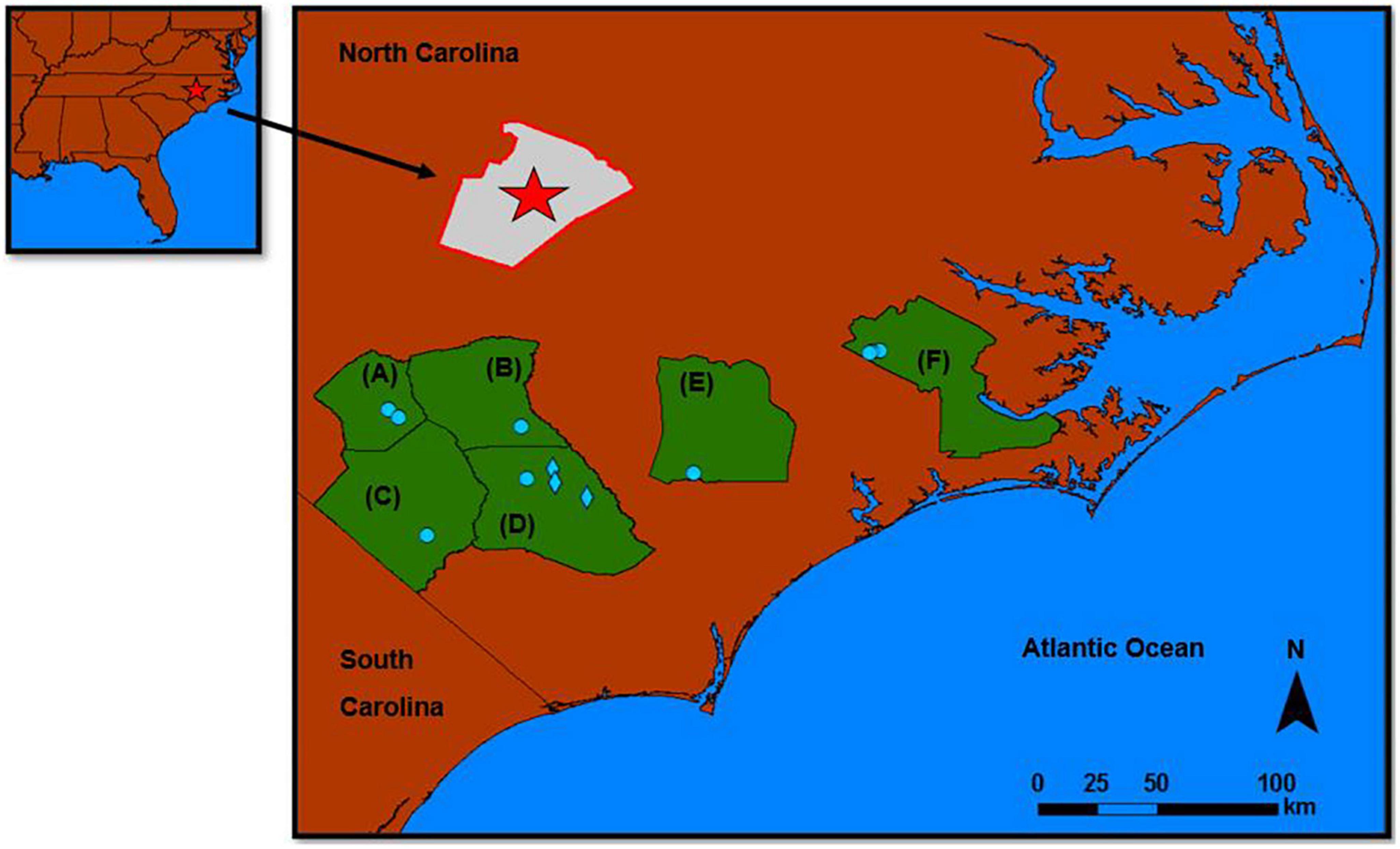
Figure 1. Locations of the Carolina Bay research sites in relation to Raleigh, NC (red star). Mitigation sites are shown as blue circles and reference sites are shown as blue diamonds. (A) Hoke County–Arabia Bay and Hillcrest Bay, (B) Cumberland County–Barra Farms (Harrison Bay), (C) Robeson County–Juniper Bay, (D) Bladen County–Dowd Dairy and Reference Bays (Causeway, Charlie Long-Millpond, and Tatum-Millpond Bays), (E) Duplin County–Twin Bays, and (F) Craven County -Dover Bay and Sliver moon 1 and 2.

TABLE 1

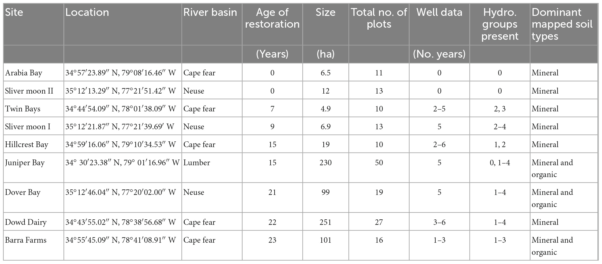
Table 1. Site characteristics for nine Carolina Bay mitigation sites.

Water table levels were monitored at the restoration sites using wells that were constructed and installed following the US Army Corps of Engineer guidelines (US Army Corps of Engineers [USACE], 2005). Water table measurements were recorded daily using automated groundwater gauges. In general, 5 years of well data were collected at the sites and the maximum consecutive days of saturation within 30 cm of the soil surface during the growing season in 5 years of 10 (50% probability) were reported. An average of the 5 years of hydrologic data was computed and each well location was categorized into one of the four Hydrologic Groups as defined by Moritz et al. (2022). Saturation periods for the Groups were: (1) < 14 (non-wetland areas), (2) 14–50, (3) 51–100, and (4) 101+ days of saturation. In most cases, the average period of saturation was obtained from 5 years of well data obtained from the NCDEQ-DMS database (NC Department of Environmental Quality [NCDEQ], 2020; Table 1).

Soil sampling

The study sites were sampled in 2019 and 2020. For each site, the well data were first examined to place each well into one of the four Hydrologic Groups. Points were georeferenced in ArcMap (Esri, 2016) from site maps found within the NCDEQ-DMS mitigation reports and from Ewing et al. (2012). The plots were located in the field using a global navigation satellite system with a Trimble: Nomad and a Trimble: GeoXT (Trimble Inc., Sunnyvale, CA, USA). In general, five plots within each Hydrologic Group were sampled at each site location. Most of the plots were placed within 2 m of a well or an old well location if the well had been removed. In a few cases, a given Hydrologic Group at a site contained only three wells. Two more plots were then identified approximately 30 to 500 m away from a well by extrapolating hydrologic data across the site using a 2-D spline analysis in ArcMap based on the techniques used by Moritz et al. (2022). Sites that had not been restored were sampled along transects positioned across a soil map unit and/or were sampled at proposed well locations.

For sampling plots that were not inundated, two to three soil pits were dug (30 cm wide and 30 cm deep) 1 m apart with a spade. Saturated organic and/or mineral soils, which could not be sampled by spade, were sampled with a McCauley auger and/or an open bucket auger. Soil profiles were described by soil horizon on vertical sections removed from the pits and/or from soil carefully removed from the augers. Profile descriptions included horizon depth, Munsell color of the matrix, soil texture, and redoximorphic features. These data were used to determine whether hydric soil field indicators were present, and only the occurrence of the field indicators will be reported here.

Litter thickness was measured at each pit location before the pit was dug. In general, sites that had been restored for ≤ 9 years had not reached tree crown closure, and the litter layer did not fully cover the ground. Litter thickness in these areas was generally measured at 1/3 the length to the full length of the lowest main branch on the nearest tree, located near the center of the plot. Site microtopography, and disturbance within the plot were also determined where the litter layer was measured. For sampling sites that were inundated, two to three auger borings were made 1 m apart with an open bucket auger and/or a McCauley auger down to 30 cm. When litter thickness was assessed underwater, the top of the litter layer was determined by hand and the depth to the original soil surface was measured by tape.

Anaerobic and hydrologic determination

US Army Corps of Engineers [USACE] (2010) wetland hydrology field indicators were identified at the plots at time of sampling. The total number of all hydrology indicators found, as well as the specific indicators that were found in at least 50% of the plots within a given Hydrologic Group were used in our analyses. Indicator of Reduction in Soils (IRIS) tubes were installed with a push probe at selected plots within each Hydrologic Group at the restored sites to confirm that saturation and anaerobic conditions occurred at the sites. Five IRIS tubes were inserted into the soil over an area that was < 2 m in diameter and near the sampling plots (Berkowitz, 2009). In general, the IRIS tubes were left in the ground for about 8 months at Juniper Bay. The remaining six sites that were restored (Table 1) had tubes left in the ground for about 6 months. The average area of Fe-oxide paint removed was estimated by eye to a depth of 30 cm.

Vegetation assessments

Vegetation was assessed in each of the five plots per Hydrologic Group at a site. Basal area was determined in a variable radius plot using a 10-factor prism on trees with a diameter at breast height (DBH) ≤ 5 cm. Tree species were identified on all trees within the variable radius plot. A tree species was considered dominant if the given species composition was > 19.4% across all plots for a given Hydrologic Group, within a given site. Fixed radius plots with a radius of 5.64 m (1/100 ha) were used to determine species for shrubs, vines, saplings, and seedlings that were needed to confirm wetland hydrology field indicator (D5), FAC-neutral test (US Army Corps of Engineers [USACE], 2010). Graminoids were also noted and were dominantly Carex spp., Juncus spp., and Typha spp. Indicator statuses for plants were determined using the USDA-NRCS PLANTS database search engine (United States Department of Agriculture – Natural Resources Conservation [USDA-NRC], 2020).

Potential tree height was determined for a healthy tree within a plot. The potential tree height is the representative tree height on a healthy tree that was a dominant species within the plot. Potential tree height was determined by taking one-half of the sum of the slope (in percent) from eye level to the top of the tree and from the base of the tree at a point 15 m from the tree (DeYoung, 2018). A healthy tree was chosen based on it representing a dominant tree species in the plot, the tree did not have a broken top, the crown was not forked, and the tree was straight. Percent slope was quantified using a clinometer. Variables related to aboveground biomass and litter layer thickness (i.e., variables related to organic carbon) were measured at all plots, not selected plots described above.

Reference Carolina Bays

Three organic soil based Carolina Bays located in Bladen County, NC that had not burned or been logged for at least 65 years were used as reference sites (Dimick et al., 2010). Previous work characterized the hydrology (Caldwell et al., 2011), soils (Ewing et al., 2012), and vegetation (Dimick et al., 2010). The Bays were named Charlie Long−Millpond Bay (34°46′04.96″ N, 78°33′36.24″ W), Tatum Millpond Bay (34°43′00.09″ N, 78°33′05.95″ W), and Causeway Bay (34°39′41.92″ N, 78°25′45.13″ W) (Figure 1).

Statistical analyses

The total number of hydrology indicators and IRIS tube Fe-oxide paint removal were analyzed using analysis of variance (ANOVA) in SAS 9.4 using the PROC GLM function with Tukey Kramer’s multiple comparison procedure to test pairwise differences between the Hydrologic Groups (SAS, 2013). Least-square means (LSMEANS) were used because the data were not balanced. Within site comparisons between Hydrologic Groups and between site comparisons within a given Group with C-based variables (i.e., litter thickness, potential tree height, and tree basal area) were also analyzed using ANOVA with Tukey Kramer’s multiple comparison procedure using LSMEANS.

Litter layer thickness, and tree basal area and height were regressed across short-term chronosequences (0–23 years) for each Hydrologic Group using the PROC GLM function in SAS (SAS Institute, 2013, Cary, NC). Measured variables were transformed by taking the square-root of the measured value to help stabilize the variance and/or increase the accuracy of the model. All regressions were fixed to zero to mimic natural conditions at the time of restoration. Multiple zero points (i.e., data from sites that have not been restored, 24 data points) were not inserted into the model(s) to avoid high leverage from the zero points.

Predicted values for ages 1 to 25 years from each short-term chronosequence, for a given variable from each Hydrologic Group, were also analyzed through ANOVA using the PROC GLM function in SAS 9.4 (SAS Institute, 2013, Cary, NC). Hydrologic Groups were used as a class. Tukey Kramer’s multiple comparison procedure was used to compare LSMEANS between the Groups to see if the regression slopes between the Hydrologic Groups were significantly different.

Regressions to estimate the maximum consecutive days of saturation during the growing season were created using PROC GLM in SAS (SAS Institute, 2013, Cary NC). The total number of hydrology indicators, age of restoration, litter layer thickness, tree basal area, potential tree height, and the presence of organic soils and/or soils with a histic epipedon based on definition 1b (i.e., surface organic thickness ranges from 20 to 40 cm, Soil Survey Staff, 2014) were used as predictors in the regressions.

Folded F-tests, plotting the residuals against the fitted values, and/or Q-Q plots were assessed to see if the data contained a constant variance and to see if the data were normal. Square-root transformations were used to help stabilize the variance within the chronosequences. All comparisons were made at the 0.05 level unless noted otherwise.

Results

Hydrology and vegetation

Hydrologic and soil properties are summarized in Table 2. The average maximum consecutive days of saturation during the growing season were used to define Hydrologic Groups. The total number of hydrology field indicators increased in going from Hydrologic Group 1 (3 indicators) to Hydrologic Group 4 (8 indicators). Hydrology indicators A3 (saturation), D2 (geomorphic position), and D5 (FAC-neutral test) were found in at least 50% of the plots in all Hydrologic Groups.

TABLE 2

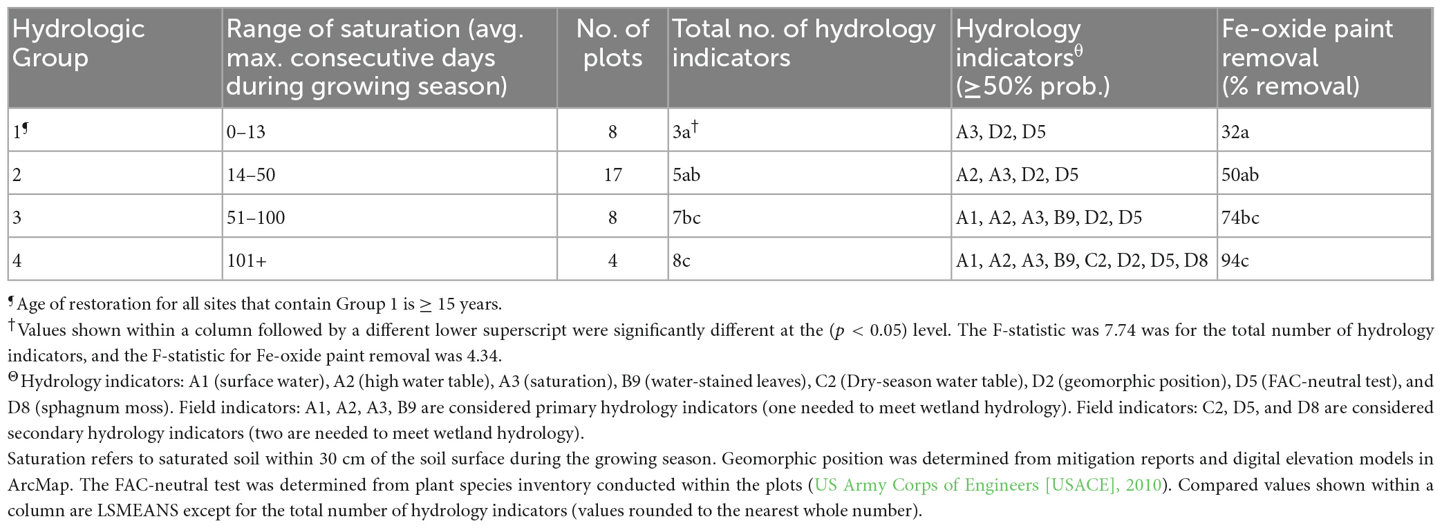
Table 2. Summary of hydrologic and soil properties found in plots where IRIS tubes were installed.

The IRIS tubes confirmed that saturation and anaerobic conditions occurred in the soils examined (Table 2) across all Hydrologic Groups. In general, the higher percentage of Fe-oxide paint removal corresponds to longer periods of anaerobic conditions and Fe reduction. Plots that experienced saturation durations for > 100 days had significantly (p < 0.05) more Fe oxide paint removed (94% removal) from the IRIS tubes than areas that experienced saturation periods < 51 days (32 and 50% removal). Hydrologic Group 3 experienced significantly (p < 0.05) more Fe oxide paint removal (74% removal) than Group 1 (32% removal). These results confirmed that durations of saturation and anaerobic conditions increased progressively from Hydrologic Groups 1 to 4.

Mean values found for litter thickness, basal area, and potential tree height in the reference bays for each Hydrologic Group are shown in Table 3. Reference means are compared to mean values for the restored sites at 23 years (Groups 1–3) and 21 years (Group 4) after restoration. Data for litter (Ewing et al., 2012) and tree basal area (Dimick et al., 2010) were obtained from the previous studies done at the reference bay plots used for this study. Potential tree height data were obtained by Hall and Penfound (1939) and Otte (1982), as such data were not collected at the reference bays. The restored sites had litter thicknesses similar to those of the reference sites in Groups 1 and 2 (12 vs. 10 cm, and 13 vs. 10 cm) but not in Groups 3 and 4 (15 vs. 23 cm, and 19 vs. 40 cm) (Table 3). In general, tree basal area values at the restoration sites were about half of those found at the reference locations. Values for potential tree height in the restored sites were similar to those found for canopy height in the reference bays for Hydrologic Groups 1, 2, and 4 (7 to 17 m vs. 10 to 18 m). In Hydrologic Group 3, the potential tree height was approximately 9 m less (16 m) in the restoration site at 21 years than the canopy height found in the reference bays (25 m) (Table 3).

TABLE 3

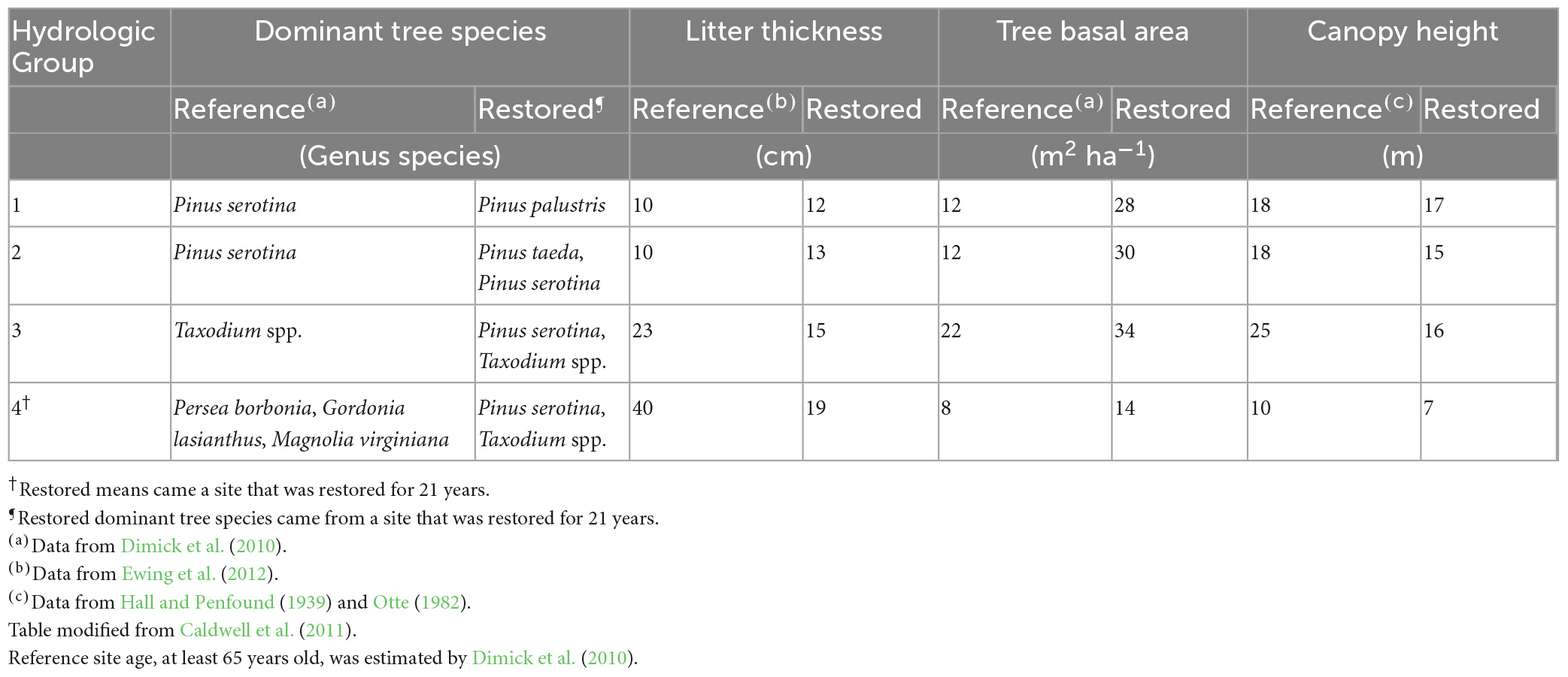
Table 3. Reference means and restored means found 23 years after restoration for major site parameters.

Regression equations developed to estimate the maximum consecutive days of saturation at the sites are shown in Table 4. Multiple regression and interactive models (R² = 0.57–0.73 and p = 0.05 to p < 0.001) were developed with the total number of hydrology indicators, age of restoration, litter layer thickness, potential tree height, and organic soils and/or soils with a histic epipedon based on definition 1b (i.e., surface organic thickness ranges from 20 to 40 cm) (Soil Survey Staff, 2014). While the regression results show that maximum consecutive days of saturation could be estimated using a host of vegetation, site, and soil properties, the easiest approach would be to simply note the total number of hydrology field indicators and place the site in a Hydrologic Group.

TABLE 4

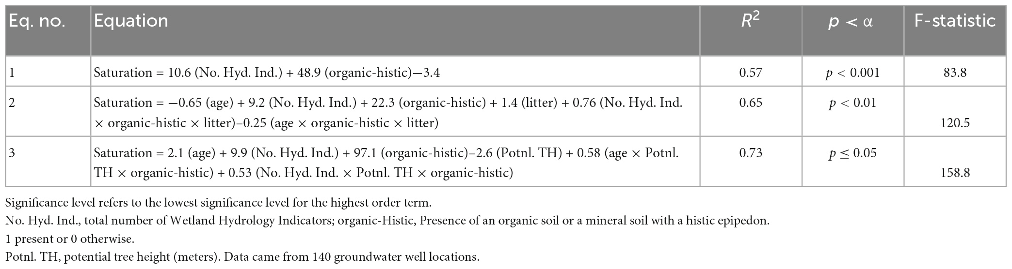
Table 4. Regressions that estimate the maximum consecutive days of saturation within 30 cm of the soil surface during the growing season.

Chronosequences

Changes in litter thickness over time are shown in Figure 2, and in Supplementary Tables 1, 2. Data were best fit with a 2nd-order polynomial term using a square root transformation. All models were significant at the 0.05 level or higher. Regression results were similar for Hydrologic Groups 1 and 2 and their data were combined in Figure 2A. Regression results were similar for Hydrologic Groups 3 and 4 and the data for these were combined as well in Figure 2B. For all Hydrologic Groups, litter thickness progressively increased up to approximately 15 years following restoration, and then remained nearly constant thereafter. Canopy closure probably occurred at about 15 years which maximized annual litter production.

FIGURE 2

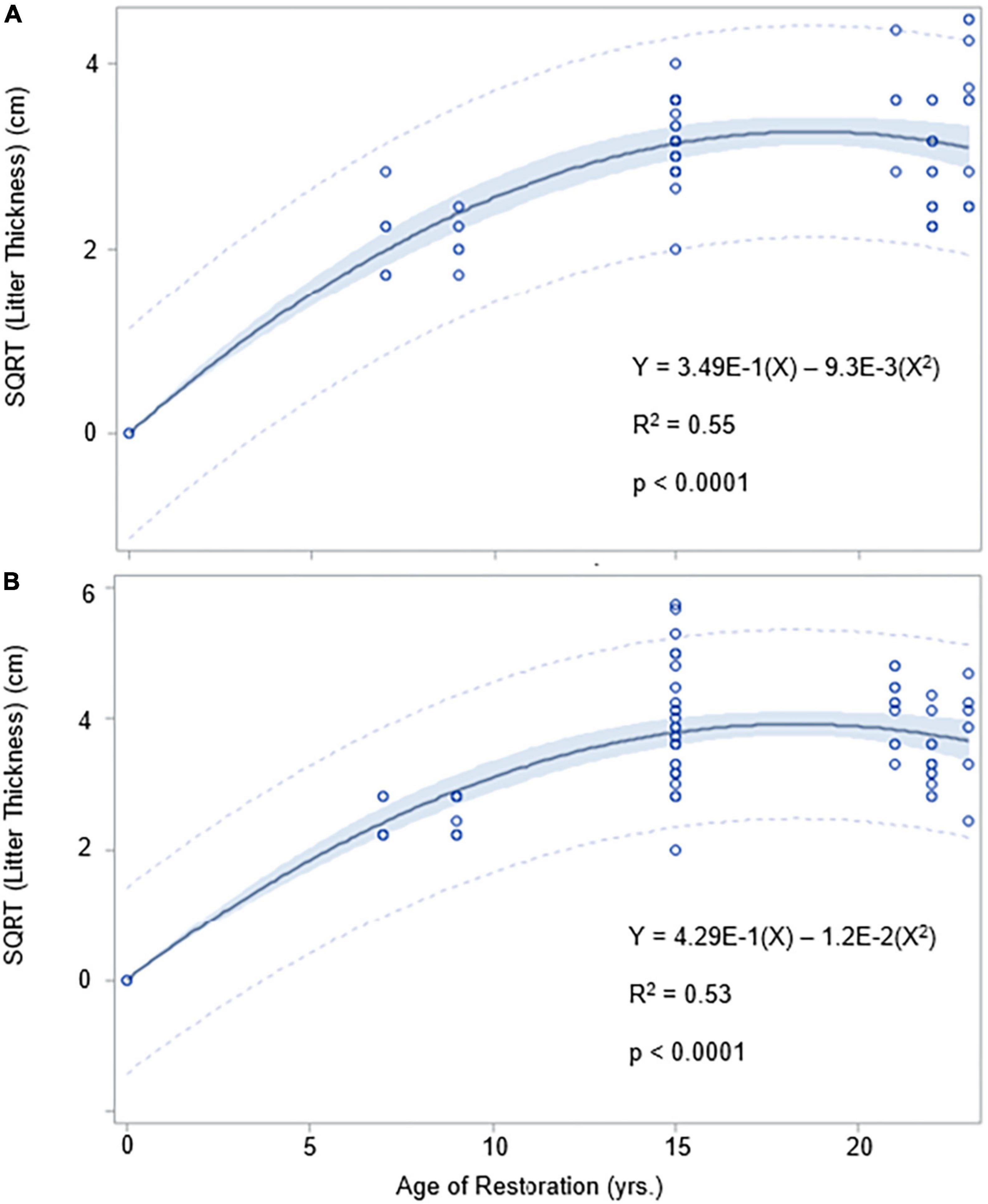
Figure 2. Chronosequences for litter layer thickness (cm) showing results for: (A) Hydrologic Groups 1 and 2, and (B) Hydrologic Groups 3 and 4. Light blue shaded areas are 95% confidence limits and areas in between the dotted lines are 95% prediction limits.

Changes in tree basal area over time are shown in Figure 3, and in Supplementary Tables 1, 2. Hydrologic Groups 1 and 2 had patterns similar to those found for litter thickness in that the curvilinear models showed basal area peaking at approximately 15 years (28 and 30 m² ha^–1) and remaining nearly constant thereafter. On the other hand, linear models best fit the data for Hydrologic Groups 3 (34 m² ha^–1) and 4 (14 m² ha^–1), and it was not clear that maximum values had been reached.

FIGURE 3

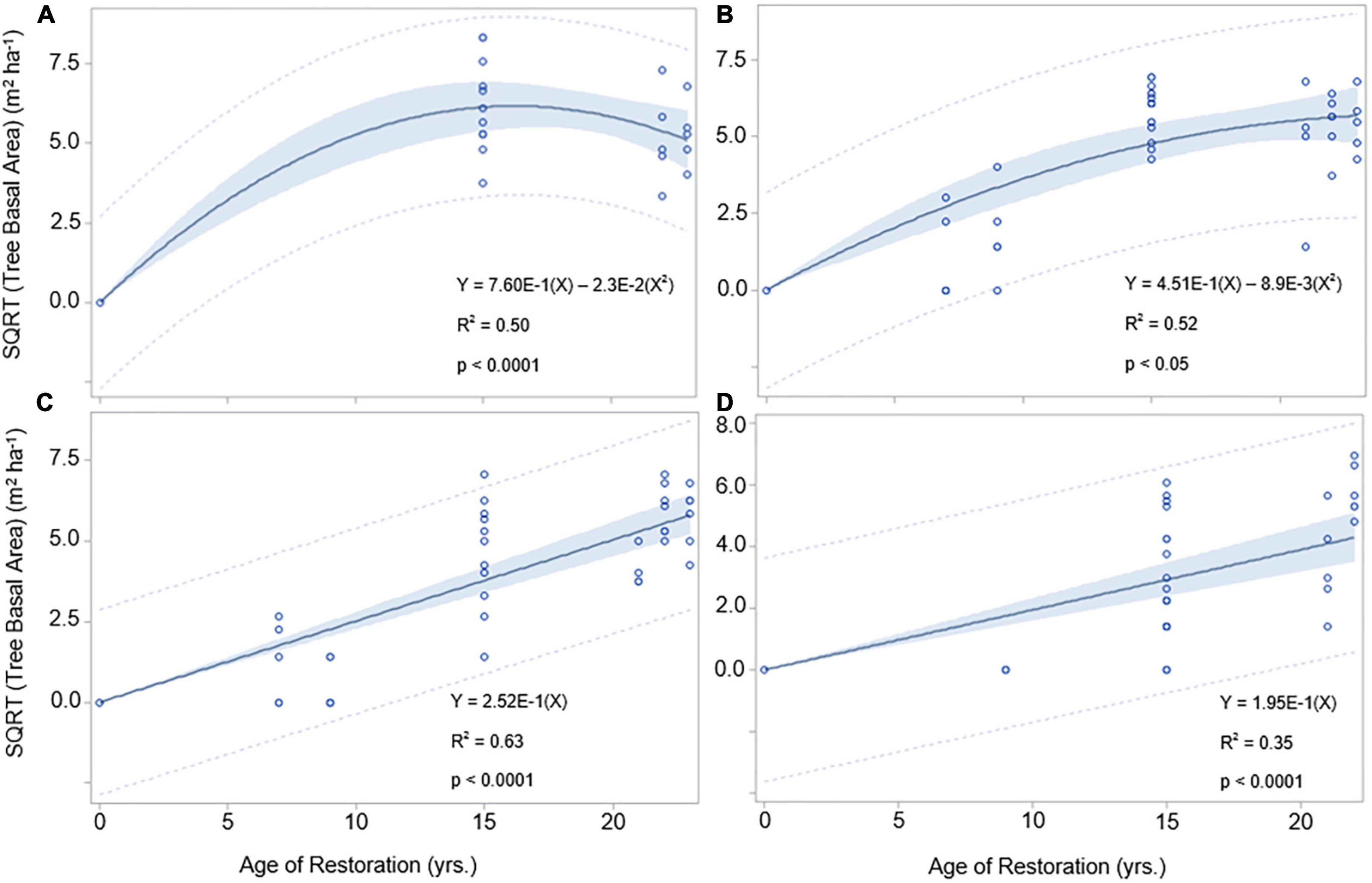
Figure 3. Chronosequences for tree basal area (m² ha^{– 1}) across four Hydrologic Groups: (A) Group 1, (B) Group 2, (C) Group 3, and (D) Group 4. Light blue shaded areas are 95% confidence limits and areas in between the dotted lines are 95% prediction limits.

Changes in potential tree height over time are shown in Figure 4, and in Supplementary Tables 1, 2. Similar curvilinear relationships were found for Hydrologic Groups 1 and 2, and for Groups 3 and 4. The potential tree height peaked at approximately 15 years reaching values of about 17 m (Groups 1 and 2) and 12 m (Groups 3 and 4).

FIGURE 4

Figure 4. Chronosequences for potential tree height (m): (A) Group 1 and Group 2 datasets are combined, (B) Group 3 and Group 4 datasets are combined. Light blue shaded areas are 95% confidence limits and areas in between the dotted lines are 95% prediction limits.

Discussion

Chronosequences

The results of the study showed that the restored Carolina Bays have not fully reached reference conditions after 23 years of restoration for every measured site parameter within each Hydrologic Group. Litter thicknesses in Hydrologic Groups 1 and 2 were similar to the reference sites after 23 years. However, litter thicknesses for Hydrologic Groups 3 and 4 were almost half those of the reference sites. Litter thickness could potentially increase over time in Hydrologic Groups 3 and 4, but these locations would probably have to experience some inundation to reduce decomposition. As shown in Table 2, hydrologic indicators of ponded conditions (e.g., A1 and B9) were observed in Hydrologic Groups 3 and 4 in 50% of the plots, but not in the other Groups. This suggests that litter thicknesses in Hydrologic Groups 3 and 4 will continue to increase at the restoration sites that become inundated.

Tree basal area values were above those found in the reference bays studied by Dimick et al. (2010). This suggested that as the restored sites age some of the trees will die. The restoration process overplants trees to compensate for those which will die during the early years of restoration. Like litter thickness, potential tree height in the restored sites at 23 years was similar to the estimated canopy height for the reference areas studied by Hall and Penfound (1939) and Otte (1982) in Hydrologic Groups 1 and 2. However, changes in potential tree height may occur in Hydrologic Groups 3 and 4. Tree height in Group 3 may increase while that in Group 4 may decrease over time as the dominant species in each group change. Presence or absence of fire (Ash et al., 1983; Schafale and Weakley, 1990), soil type, and soil fertility (Otte, 1982; Schafale and Weakley, 1990; Richardson, 2003) will likely influence how the litter thickness and vegetation characteristics change over longer time periods (Supplementary Figures 1–3). Sueltenfuss and Cooper (2019) found that even though wetland hydrology can be restored to mimic reference conditions, the plant communities that grow in the mitigation sites do not lead to similar plant communities found in reference systems.

Ecological assessment

The results of this study have not been validated at other Carolina Bay locations, but they could potentially be used to evaluate restoration sites that have a similar landform and hydrology, and if the site previously experienced agriculture. The relationships shown in Figures 2–4 and Table 4 might be used to aid field personnel in evaluating restoration sites of different ages in similar Carolina Bay wetlands. Each of the restoration sites represented restorations with appropriate hydrology, vegetation, and soil conditions needed for a potentially successful restoration (except for Hillcrest Bay, which was primarily used for Group 1−non-wetland areas). Field personnel could use the data in Figures 2–4, Table 4, and Supplementary Table 3 by first considering the age of a given restoration site. Vegetation plots in the restored wetland should then be selected along a transect that likely contains a wetness gradient that may include Hydrologic Groups 1 to 4. Hydrologic field indicators should be identified at the selected plots and compared to monitoring well data if available to confirm the Hydrologic Group. General soil type can be estimated using a push probe to determine if the soils are organic or contain a histic epipedon according to definition 1b (Soil Survey Staff, 2014). Litter thickness, basal area, and potential tree height (if trees are present) can be quickly estimated on site.

Where groundwater well data are not available, Hydrologic Groups could be estimated using the total number of field indicators and type (Table 2) found in the plots at the restored sites. The equations shown in Table 4 offer an additional way to estimate saturation duration, but the equations need additional verification at other sites before widespread usage can be recommended. Once the Hydrologic Group is known, litter layer thickness, tree basal area and height can be plotted in Figures 2–4. If a restored site’s average values for litter thickness, tree basal area, and potential tree height within a given Group fall within the 95% confidence limits shown, then the site might be considered adequately restored for its age. However, if the values of any parameter fell below or above the 95% confidence limits, then project goals should be reassessed. This could consist of manipulating the hydrology and/or planting additional trees to meet project goals. More studies need to be done to verify the results in Figures 2–4 and Tables 3, 4. However, the results reported here show that the chronosequences have the potential to be a useful tool for evaluating Carolina Bay restoration sites.

Conclusion

Nine Carolina Bay restoration sites were compared for changes in litter thickness, basal area, and potential tree height over time. Carolina Bays were focused on because it was assumed that all sites would undergo similar changes over time for a given Hydrologic Group, and there are no ecological assessments currently available for this landform. Time since restoration ranged from 0 to 23 years with restoration sites that were considered to have hydrology, plants and soil conditions found in Carolina Bays, except for one site that was primarily used for non-wetland areas.

In general, litter thickness increased over time and appeared to reach an equilibrium at approximately 15 years. Wetland plots saturated for ≥ 51 days during the growing season had litter thicknesses about half of what was found in reference sites for similar saturation periods. Plots saturated for < 51 days during the growing season had litter thicknesses that were similar to reference sites. Inundation during the growing season occurred in ≥ 50% of the plots that were saturated for ≥ 51 days and was expected to reduce decomposition of litter enough to allow litter thickness to increase over time.

Tree basal area increased with time up to 15 years for sites saturated < 51 days during the growing season. For sites saturated for longer periods, basal area appeared to increase up to approximately 23 years following restoration. Tree basal areas at the restored sites were about one half of those of the reference sites, which suggested that some trees at the restored sites will eventually die off.

Potential tree height increased with time up to 15 years in the restored sites that were saturated for ≤ 100 days during the growing season. For sites saturated for > 100 days during the growing season, potential tree height continued to increase up to 23 years following restoration. Potential tree height at 15 to 23 years of restoration was similar to canopy height in reference sites in plots saturated for < 51 days during the growing season. Potential tree height (at 23 years) in plots saturated for 51 to 100 days during the growing season was less than canopy height in reference sites. For restored sites saturated > 100 days during the growing season, potential tree height was slightly greater than the canopy height estimated for reference sites. Further research is needed on older restoration sites to determine how tree species will change over time in the latter two groups. The chronosequences and saturation regressions developed here will be useful to field personnel who evaluate wetland restoration conditions in restored Carolina Bays.

Data availability statement

The original contributions presented in this study are included in the article/Supplementary material, further inquiries can be directed to the corresponding author.

Author contributions

CM completed field work and data analyses, and contributed to the manuscript preparation. MV secured funding, developed the research plan, assisted in data analyses, and contributed to the manuscript preparation. MR assisted in planning the research and securing funding, and edited the manuscript. All authors contributed to the article and approved the submitted version.

Funding

United States Department of Agriculture, Natural Resources Conservation Service supplied all funding for the project through NR1874820006C003. They have agreed to pay the publication fees pending review and acceptance of the manuscript.

Acknowledgments

United States Department of Agriculture, Natural Resources Conservation Service personnel assisted with collecting vegetation data and their help is greatly appreciated.

Conflict of interest

The authors declare that the research was conducted in the absence of any commercial or financial relationships that could be construed as a potential conflict of interest.

Publisher’s note

All claims expressed in this article are solely those of the authors and do not necessarily represent those of their affiliated organizations, or those of the publisher, the editors and the reviewers. Any product that may be evaluated in this article, or claim that may be made by its manufacturer, is not guaranteed or endorsed by the publisher.

Supplementary material

The Supplementary Material for this article can be found online at: https://www.frontiersin.org/articles/10.3389/ffgc.2023.1148935/full#supplementary-material

References

Ash, A., McDonald, E., Kane, E., and Pories, C. (1983). Natural and modified pocosins: Literature synthesis and management options. Washington, DC: US Fish and Wildlife Services.

Google Scholar

Berkowitz, J. (2009). Using IRIS tubes to monitor reduced conditions in soils - project design. Wetlands Regul. Assist. Progr. 9, 1–10.

Google Scholar

Caldwell, P., Vepraskas, M., Gregory, J., Skaggs, R., and Huffman, R. (2011). Linking plant ecology and long-term hydrology to improve wetland restoration success. Adv. For. Hydrol. 54, 2129–2137. doi: 10.13031/2013.40662

CrossRef Full Text | Google Scholar

De Steven, D., and Lowrance, R. (2011). Agricultural conservation practices and wetland ecosystem services in the wetland-rich Piedmont-Coastal Plain region. Ecol. Applic. 21, S3–S17. doi: 10.1890/09-0231.1

CrossRef Full Text | Google Scholar

DeYoung, J. (2018). “Forest measurements: An applied approach,” in Field technique tips for measuring tree height, 1st Edn, ed. J. DeYoung (Morrisville, NC: Open Oregon Educational Resources), 55–61.

Google Scholar

Dimick, B. P., Stucky, J., Wall, W., Vepraskas, M., Wentworth, T., and Arellana, C. (2010). Plant-soil-hydrology relationships in three Carolina bays in Bladen County, North Carolina, USA. Castanaea 75, 407–420. doi: 10.2179/09-063.1

CrossRef Full Text | Google Scholar

Esri (2016). Arcmap version 10.4. Redlands, CA: Esri Products.

Google Scholar

Ewing, J., Vepraskas, M., and Zanner, C. (2005). Using historical records of land use to improve wetland mitigation. Southeast. Geogr. 45, 25–43. doi: 10.1353/sgo.2005.0005

PubMed Abstract | CrossRef Full Text | Google Scholar

Ewing, J., Vepraskas, M., White, J., and Broome, S. (2012). Changes in wetland soil morphological and chemical properties after 15, 20, and 30 years of agricultural production. Geoderma 179-180, 73–80. doi: 10.1016/j.geoderma.2012.02.018

CrossRef Full Text | Google Scholar

Fennessy, M., Gernes, J., Mack, J., and Wardrop, D. (2001). Methods for evaluating wetland condition: Using vegetation to assess environmental conditions in wetlands. Washington, DC: US Environmental Protection Agency, Office of Water.

Google Scholar

Fennessy, S., Jacobs, A., and Kentula, M. (2007). An evaluation of rapid methods for assessing the ecological condition of wetlands. Wetlands 27, 504–521. doi: 10.1672/0277-5212(2007)27[543:AEORMF]2.0.CO;2

CrossRef Full Text | Google Scholar

Gil-Sotres, F., Trasar-Cepeda, C., Leiros, M., and Seoane, S. (2005). Different approaches to evaluating soil quality using biochemical properties. Soil Biol. Biogeochem. 37, 877–887. doi: 10.1016/j.soilbio.2004.10.003

CrossRef Full Text | Google Scholar

Hall, T., and Penfound, W. (1939). A phytosociological study of a Nyssa biflora consocies in southeastern Louisiana. Am. Midland Nat. 22, 369–375. doi: 10.2307/2420315

CrossRef Full Text | Google Scholar

Kusler, J., and Kentula, M. (1990). “Executive summary,” in wetland creation and restoration: The status of the science, eds J. A. Kusler and M. E. Kentula (Washington, DC: Island Press).

Google Scholar

Mitsch, W., and Gosselink, J. (2007). Wetlands, 4th Edn. New York, NY: John Wiley & Sons.

Google Scholar

Moon, J., and Wardrop, D. (2013). “Linking landscapes to wetland condition,” in Mid-atlantic freshwater wetlands: Advances in wetlands science, management, policy, and practice, eds R. Brooks and D. Wardrop (New York, NY: Springer Publishing), 61–108. doi: 10.1007/978-1-4614-5596-7_3

CrossRef Full Text | Google Scholar

Moritz, C. M., Vepraskas, M. J., and Ricker, M. C. (2022). Hydrology and vegetation relationships in a Carolina bay wetland 15 years after restoration. Wetlands 42:8. doi: 10.1007/s13157-022-01530-0

CrossRef Full Text | Google Scholar

National Research Council [NRC] (1995). Wetlands: Characteristics and boundaries. Washington, DC: National Academy Press.

Google Scholar

NC Department of Environmental Quality [NCDEQ] (2013). NC ecosystem enhancement program celebrates a decade of conserving and restoring streams and wetlands. Available online at: https://deq.nc.gov/press-release/nc-ecosystem-enhancement-program-celebrates-decade-conserving-and-restoring-streams (accessed August 3, 2020).

Google Scholar

NC Department of Environmental Quality [NCDEQ], (2020). Division of mitigation services projects. Available online at: https://deq.nc.gov/division-mitigation-services-projects (accessed May 29, 2023).

Google Scholar

Otte, L. (1982). Origin, development, and maintenance of the pocosin wetlands of North Carolina. Raleigh, NC: North Carolina Natural Heritage Program.

Google Scholar

Prouty, W. (1952). Carolina bays and their origin. Geol. Soc. Am. Bull. 63, 167–224. doi: 10.1130/0016-7606(1952)63[167:CBATO]2.0.CO;2

CrossRef Full Text | Google Scholar

Richardson, C. (2003). Pocosins: Hydrologically isolated or integrated wetlands on the landscape. Wetlands 23, 563–576. doi: 10.1672/0277-5212(2003)023[0563:PHIOIW]2.0.CO;2

CrossRef Full Text | Google Scholar

SAS (2013). Statistical analysis software. Users’ guide statistics version 9.4. Cary, NC: SAS Institute.

Google Scholar

Schafale, M., and Weakley, A. (1990). Classification of the natural communities of North Carolina. Raleigh, NC: North Carolina Natural Heritage Program.

Google Scholar

Schloter, M., O’Dilly, C., and Munch, J. (2003). Indicators for evaluating soil quality. Agric. Ecosyst. Environ. 98, 255–262. doi: 10.1016/S0167-8809(03)00085-9

CrossRef Full Text | Google Scholar

Sharitz, R. R. and Gibbons, J. W. (1982). The ecology of southeastern shrub bogs (pocosins) and Carolina bays: A community profile. FWS/OBS 82/04. Washington, DC: U.S. Fish and Wildlife Service, Division of Biological Services. Available online at: http://pubs.er.usgs.gov/publication/fwsobs82_04

Google Scholar

Soil Survey Staff (2014). Keys to soil taxonomy, 12th Edn. Washington, DC: USDA-NRCS.

Google Scholar

Sueltenfuss, J., and Cooper, D. (2019). Hydrologic similarity to reference wetlands does not lead to similar plant communities in restored wetlands. Restor. Ecol. 27, 11137–11144. doi: 10.1111/rec.12964

CrossRef Full Text | Google Scholar

United States Army Corps of Engineers (2002). Regulatory guidance letter no. 02-2. Available online at: https://www.epa.gov/sites/default/files/2015-08/documents/mitigation_rgl_02-2_0.pdf (accessed May 29, 2023).

Google Scholar

US Army Corps of Engineers [USACE] (2005). Technical standard for water-table monitoring of potential wetland sites wrap technical notes collection. Vicksburg, MS: US Army Engineer Research and Development Center.

Google Scholar

US Army Corps of Engineers [USACE] (2010). Regional supplement to the corps of engineers wetland delineation manual: Atlantic and gulf coastal plain region (version 2.0). Vicksburg, MS: US Army Engineer Research and Development Center.

Google Scholar

United States Department of Agriculture – Natural Resources Conservation [USDA-NRC] (1994). National food security act manual, third edition (as amended). Washington, DC: USDA Natural Resources Conservation Service.

Google Scholar

United States Department of Agriculture – Natural Resources Conservation [USDA-NRC] (2020). Plant database search engine. Available online at: https://plants.usda.gov/java/ (accessed May 29, 2023).

Google Scholar

United States Department of Agriculture [USDA] (2002). Wetland reserve program: Restoring America’s wetlands. Washington, DC: USDA Natural Resources Conservation Service.

Google Scholar

Wardrop, D., Kentula, M., Brooks, R., Fennessy, M., Chamberlain, S., Havens, K., et al. (2013). “Monitoring and assessment of wetlands: Concepts, case-studies, and lessons learned,” in Mid-Atlantic freshwater wetlands: Advances in wetlands science, management, policy, and practice, eds R. Brooks and D. Wardrop (New York, NY: Springer Publishing), 381–420. doi: 10.1007/978-1-4614-5596-7_11

CrossRef Full Text | Google Scholar