Multidimensional hydrological modeling of a forested catchment in a German low mountain range using a modular runoff and water balance model

1. Introduction

Many forests are increasingly suffering from drought stress due to the changing climatic conditions (Allen et al., 2010). Severe droughts have negatively affected forest stands in Central Europe, also in Lower Franconia, a region in Central Germany, which is very much affected by climate change (Fischer et al., 2022). Despite its great importance, the effects of drought on forests are still not fully understood (Etzold et al., 2014), especially with respect to small-scale heterogeneities in the soil and the resulting water availability (Schuldt et al., 2020; Cholet et al., 2022). There is a need for fine-scale assessments of water stress considering site conditions and vegetation parameters to guide forest management during climate change (Field et al., 2020). There are different approaches to derive recommendations considering tree species selection out of data on plant-available water in the soil. One of them is the measurement of in situ data (water content, matric potential, and field capacity), offering a direct assessment of the water supply and a subsequent derivation of management options for the surveyed forest site. Owing to the small-parcel management of Central European forests as well as the small-spatial variation of soil and stand properties, the measurement of in situ data is insufficient, as sampling needs to be carried out for each individual forest stand, which is impossible. For this reason, point data have to be interpolated, e.g., for a forest district or bigger management units, while still maintaining data quality. For this step, remote sensing methods represent an attractive additional opportunity, offering data on canopy parameters for designated areas. The products of the Terra Moderate Resolution Imaging Spectroradiometer (MODIS) offer, besides vegetation indices, improved terrestrial evaporation estimates at a spatial resolution of 500 m and on an 8-day interval since 2000 (Running et al., 2021). Considering the coarse resolution of such remote sensing products, an application of a multidimensional hydrological model is required to assess the water balance of forest stands combining spatially high-resolution soil and vegetation data with other auxiliary geodata. In the past, hydrological models were mainly used to investigate the potential effects of forest management on hydrological processes and the resulting consequences for the water balance, mostly on a catchment scale (Whitaker et al., 2002; Moore et al., 2007). In times of climate change, this view is reversed, whereby it is more important to what extent the water balance influences the forest. To date, numerous hydrological models of varying complexity and functionality are available to model the water balance, like Hydrus 1D (Šimůnek, and van Genuchten, 2008) with one spatial dimension and rather low complexity and functionality (Beckers et al., 2009a,b). As a forest-specific hydrological model, LWF-Brook90 (Hammel and Kennel, 2001) offers one spatial dimension and medium complexity and functionality (Beckers et al., 2009a,b). Although 1D hydrological models are easier to parameterize and control, they do not meet the above-mentioned requirements to link in situ data with remote sensing and other geodata products. Therefore, multidimensional catchment models, like SWAT (Arnold et al., 1998; Zhao et al., 2022), VIC (Liang et al., 1994; Hamman et al., 2018), mHM (Samaniego et al., 2010), ParFlow (Ashby and Falgout, 1996), or WaSiM-ETH (Schulla, 1997), should be considered, offering more spatial dimensions.

Owing to its high functionality, the latter can link several 3D datasets and performs more appropriate hydrological modeling (e.g., Beckers et al., 2009a,b). WaSiM-ETH is a distributed, deterministic, and mainly physically based model. It offers a raster-based hydrological catchment model with area differentiation and a modular structure (Schulla, 2021a), conducting a pixel-wise calculation of water balance variables in defined watersheds. It considers a freely scalable number of soil horizons as well as an optional groundwater interaction, river cells, and surface flow dynamics. Despite these advantages, the model handling is very complex and time-consuming regarding preprocessing and parameterization (Beckers et al., 2009a,b). Therefore, it has been sparsely tested for its applicability in forest hydrology as the model complexity is further increased by the inclusion of forests (Förster et al., 2018).

This study aimed to evaluate WaSiM-ETH as a hydrological model for assessing the water balance and identifying drought stress risks in forest sites at a spatial resolution of 30 m. Therefore, we parameterized WaSiM-ETH to model the water balance in a forested German catchment area and compared the results to in situ data recorded at a forest monitoring plot. For further verification of the results, long time series (2000–2021) of remote sensing products (e.g., MOD16A2GFv006) are investigated. In addition to the default data output of WaSiM-ETH, drought-sensitive parameters, such as the difference between potential and effective stand transpiration (T_diff) and the water balance, were calculated and analyzed. Based on our model outputs, we elaborate limitations and advantages and address different ways to verify the output data for forested catchment areas. We further make recommendations on what to consider when modeling the water balance with WaSiM-ETH in forested watersheds.

2. Materials and methods

2.1. Study site

The investigated catchment is located in the Bavarian part of the Spessart, a forest-dominated low mountain range in Central Germany (Figure 1). The draining river Aschaff is about 23 km in length contributing to the Main River at the city of Mainaschaff with a bed slope of approx. 4.7‰. The drainage basin is in total 166.57 km², and the investigated catchment at the gauge is 136.4 km². The soils of the region are characterized by Cambisols from colored sandstone. The climate is classified as temperate oceanic with cool summers and moderately cold winters. The mean annual air temperature is 8.6°C, and the mean annual precipitation sums up to 1.037 mm (reference period for Neuhütten/Spessart: 1981–2010; DWD, 2021). The forested areas are dominated by deciduous trees, represented by European Beech (Fagus sylvatica) and Sessile Oak (Quercus petraea).

FIGURE 1

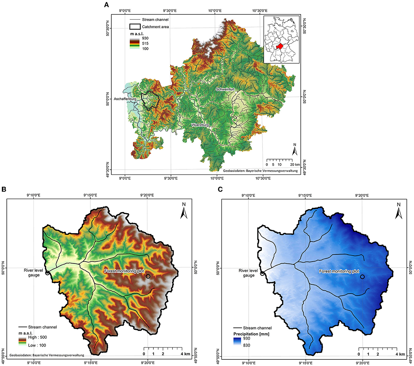
Figure 1. Topographic map of Lower Franconia (DEM 25 m, LDBV, 2021) with stream channels (A) and the catchment area of the Aschaff River with topography (B) and interpolated mean annual precipitation from 2000 to 2021 (C), including the forest monitoring plot and the river level gauge.

2.2. Parameterization and adjustment of WaSiM-ETH

2.2.1. Model description

We used WaSiM-ETH to simulate the hydrological processes within the catchment (Figure 1). The deterministic and fully distributed model is freely adjustable in terms of spatial resolution on a regular cell basis, using constant time steps and internal sub-time steps. With a focus on interpolation methods of meteorological input data, the simulation of water flux, storage, and phase transition is realized on a simplified but physically based level, with conceptual approaches. Therefore, the implemented algorithms allow users to conduct physical parameter settings. The modular structured model design offers a high variety in application possibilities and produces detailed reports of the considered processes (Schulla, 2021a).

For the present investigation, the main model features of WaSiM-ETH are evapotranspiration (ET) estimation after Penman–Monteith (Penman, 1978) and soil moisture modeling as well as runoff generation using the Richards' approach (Richards, 1931). Parameters describing the soil moisture characteristics after Van Genuchten (1980) were derived from soil maps and drill core data (Section 2.2.2) using pedotransfer functions according to Zhang et al. (2018). The landuse module of WaSiM-ETH offers a pattern-wise and seasonal-sensitive parameterization of vegetation-dependent variables (described in chapter 2.2.2). Compared to hydrological models adapted to the field, it is possible to parameterize cultivation-dependent parameters at relevant spatiotemporal scales.

2.2.2. Data

In this study, a long-term simulation from 2000 to 2021 with daily time steps was conducted. The meteorological forcing covers precipitation, air temperature, relative humidity, wind speed, and sunshine duration selected from 21 climate stations of the German Weather Service (DWD, 2022) and the Bavarian Environment Agency (BEA, 2022). A list of the used weather stations with their elevation, location, and available parameters is provided in Supplementary Table 1. The data were model-internally interpolated by a linear combination of inverse distance weighting at a maximum distance of 35 km around each station and elevation-dependent regression.

For hydrological modeling, the elevation information is the basis for topographic, morphometric, and hydrographic analysis. We used the GLO-30 Digital Elevation Model (Airbus, 2020), which represents the surface elevation of the Earth relative to the EGM2008 geoid including buildings, infrastructure, and vegetation at 30 m spatial resolution. WaSiM-ETH provides the preprocessing tool Tanalys, which creates the required elevation-derived input grids and tables to run a simulation. Detailed documentation of the used algorithms is provided by Schulla (1997, 2021a). A modified DEM using Whitebox Tools depression breaching and smoothing operations was generated to reflect the natural runoff behavior as best as possible (Lindsay, 2014). Tanalys also demands three more spatial and catchment-specific parameters to generate a spatial discretization of the catchment: (1) the coordinates of the river level gauging station, (2) a threshold value for estimating the creation of a drainage structure, and (3) the Manning–Strickler parameter, which is estimated by comparison of alike catchments. The conducted preprocessing workflow with Tanalys is depicted in Figure 2.

FIGURE 2

Figure 2. Flowchart for the processes conducted by the preprocessing tool Tanalys.

The process simulation operates in a sequential manner due to the modular construction of WaSiM-ETH. Therefore, the model interpolates the meteorological time series to grids, using inverse distance weighting with a given lapse rate. The calculation of effective ET is performed after topographic corrections of precipitation and the derivation of incoming radiation from sunshine duration. Depending on the temperature and wind speed conditions, a snow model generates additional gridded input, with consideration of gravitational slides of the simulated snowpack. The implemented interception calculation algorithm differentiates between a land use-dependent potential crop transpiration and the potential interception evaporation. First, the potential transpiration and interception from the vegetation layer and evaporation from bare soil are estimated. After the subtraction of potential snow evaporation, the effective evaporation is estimated using the relation between soil water content and the actual capillary pressure (suction) as given by the Van Genuchten parameters of the soil horizons (Schulla, 2021a). To provide the most realistic results, an internal groundwater model was enabled (Jasper et al., 2006). This gives the possibility to simulate fluctuations between the saturated and unsaturated zone. Due to the lack of observed data for groundwater levels and respective conductivities, the model needs some time to align to realistic states (swing-in phase). Following the modeling of the unsaturated conditions in the soil, the interaction of storage states of several entities (meteorological input, evaporation, snow, infiltration, and groundwater dynamics) leads to the total discharge at the outlet of the basin (c.f. Figure 3).

FIGURE 3

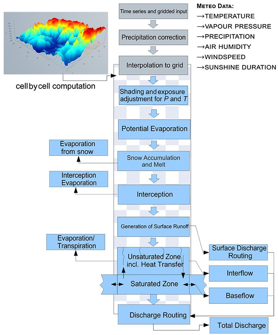
Figure 3. Sequence of the most important processing steps in WaSiM-ETH (c.f. Schulla, 2021a).

Land Cover data derived from the Landsat time series of the year 2014 provides information on nine different classes (Figure 4; resolution: 30 m) within the study area (Mack et al., 2016). Forest stands are divided into two different classes: broadleaf and coniferous woodland. These classes form the basis for the spatial assignment of vegetation-dependent variables, such as Albedo, effective vegetation height, evaporation resistance, height gradient, interception resistance, leaf area index (LAI), root density distribution, root depth, stomata resistance, and vegetation coverage. Therefore, it is possible to assign every land use-specific parameter on selected reference days to reflect seasonal changes. In this study, we used the provided parameters by Schulla (2021b).

FIGURE 4

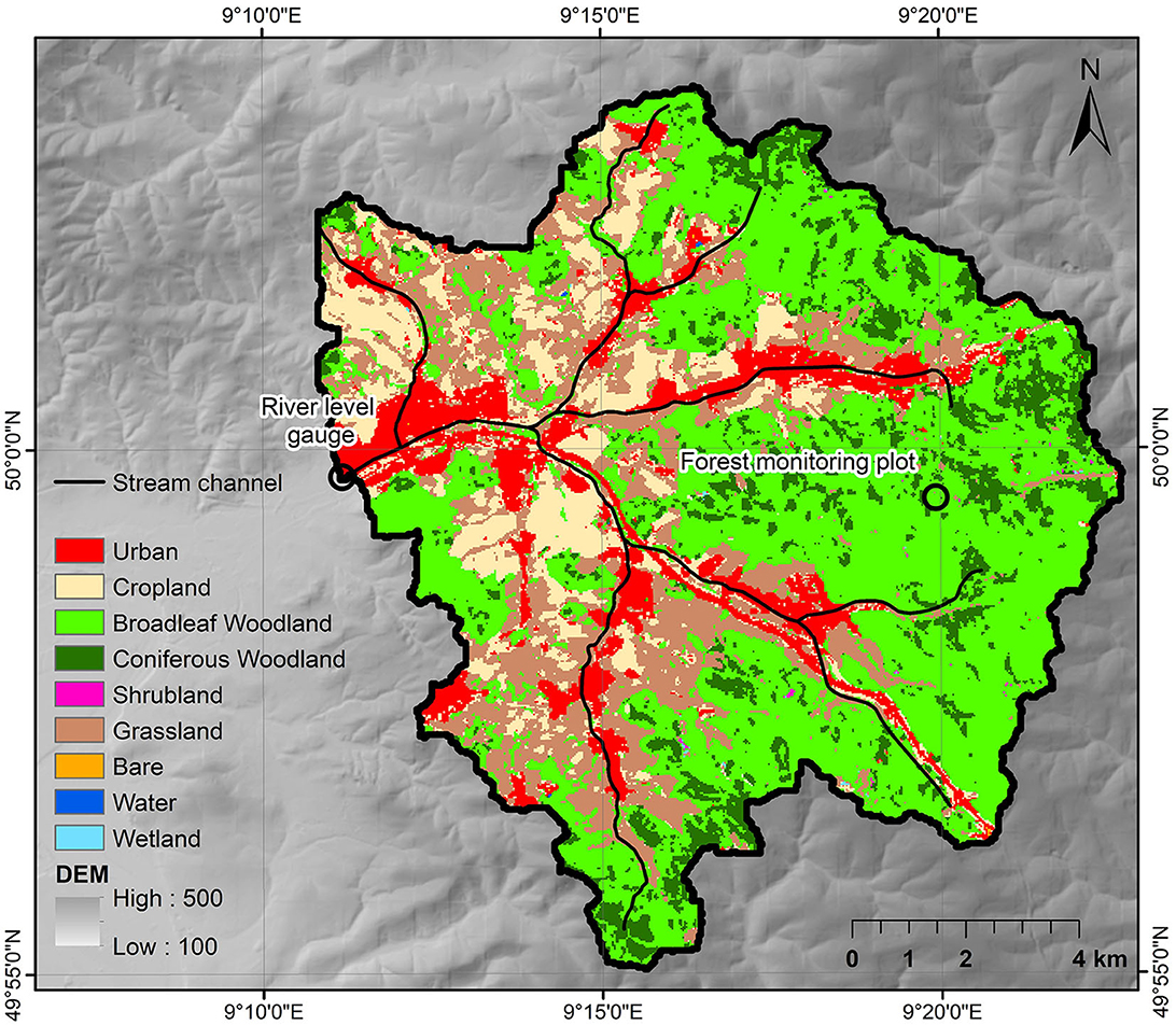
Figure 4. Landuse input provided by Mack et al. (2016) with the stream channels on a hillshade derived from the digital elevation model (GLO30) with the position of the forest monitoring plot and the river level gauge.

The used soil map was derived from BUEK200 (scale 1:200,000) and the corresponding soil database of the German Federal Institute for Geosciences and Natural Resources (BGR, 2020). All spatial data are resampled and parameterized to a grid resolution of 30 m. To predict the required soil hydraulic parameters for the unsaturated zone module, data on the grain size distribution of the BGR soil database serve as an input for ROSETTA3, which is an improved set of hierarchical pedotransfer functions based on artificial neural network (ANN) analysis coupled with bootstrap resampling methods (Zhang et al., 2018).

2.2.3. Derivation of forest drought indicators

To establish direct spatiotemporal statements regarding the water supply of forest stands, we derived two drought stress indicators that are applicable to modeled data. As the model calculates all necessary entities separately, it is possible to estimate a water balance for all forest areas according to Eq. 1.

$\begin{array}{ll}SW=P+C-Se-Su-Sl-ET& (1)\end{array}$

SW: Soil water storage change per year

P: Precipitation

C: Capillary uprise

Se: Seepage water

Su: Surface runoff

Sl: Slope water

ET: Evapotranspiration (Soil evaporation, Stand transpiration, Interception evaporation)

As another, close-to-trees drought stress indicator, we calculated the difference between potential and effective stand transpiration (Eq. 2). This indicator, also known as T_diff, is a common parameter, which has been developed for forest management by the Bavarian Institute of Forestry (LWF; Falk et al., 2008). By obtaining T_diff, an assessment of the water supply of forest stands can be made (Schultze et al., 2005; Grigoryan et al., 2010).

$\begin{array}{ll}{T}_{diff}=T_P-T_E& (2)\end{array}$

T_diff: Transpiration difference

T_P: Potential stand transpiration

T_E: Effective stand transpiration

2.3. Verification of the results

2.3.1. Evapotranspiration—MODIS data

ET rates from the MODIS MOD16A2GFv006 datasets were investigated for the period 2000–2021. This product represents an 8-day composite with 500 m spatial resolution. The variable “Total Evapotranspiration” [kg/m²/8days] is based on the logic of the Penman–Monteith equation.

2.3.2. Total runoff

The river level gauge of the Aschaff River provides daily discharge data since 1957 for the investigated catchment. The measured runoff data were converted to the area-specific discharge in mm/day. For the evaluation of the simulated discharge, we choose three different metrics, also known as goodness-of-fit measures: (1) The Kling–Gupta efficiency (KGE), (2) the coefficient of determination (R²), and (3) the volumetric efficiency (VE).

The Kling–Gupta efficiency was developed to prevent an underestimation of the runoff variability in the flows (Gupta et al., 2009). It consists of three components: the linear correlation coefficient also known as Pearson product-moment correlation coefficient (r), the ratio of the means of the simulated and observed flows (β), and the variability component (γ) as a ratio between the simulated and observed coefficient of variation. We used the modified KGE (Eq. 3) proposed by Kling et al. (2012):

$\begin{array}{ll}KGE=1-\sqrt{{(r-1)}^2+{(\beta -1)}^2+{(\gamma -1)}^2}& (3)\end{array}$

The volumetric efficiency (Eq. 4) represents the fraction of water delivered at the proper time; its complement represents the fractional volumetric mismatch (Criss and Winston, 2008).

$\begin{array}{ll}VE=1-sum(abs\left(obs-sim\right))/sum(obs))& (4)\end{array}$

The coefficient of determination is defined as the ratio of the sum of squares (SS) of the residuals (res) to the scatter of the measured (tot) data (Eq. 5).

$\begin{array}{ll}{R}^2=1-\frac{S{S}_{res}}{S{S}_{tot}}& (5)\end{array}$

All goodness-of-fit measures have their optimum at 1. The calibration process underlies an adaption of parameter settings of comparable catchments with an amount of the “trial and error” procedure (Kasei, 2010; Kassa, 2013).

2.3.3. In situ data from a forest monitoring plot

Within the catchment, a forest monitoring plot was established at the end of 2020. On this plot, a weather station was set up, consisting of a rain gauge (resolution: 0.2 mm), a temperature and relative humidity sensor (error: ±0.2°C, ±2.5 % RH), and a HOBO U30 NRC (all from the Onset Computer Corporation) logging the measurements every 10 min. To additionally measure the water content in the main rooting zone (0–1 m), three TDR probes (ECH₂O EC-5, error ±3%) obtained from the same company were installed at soil depths of 20 cm, 40 cm, and 80 cm and logged via the weather station. On a directly neighboring forest clearing, a weather station was also installed using the same configuration as indicated above. The plot was additionally equipped with totalizers (Forest plot: 5; Open area: 3) and two stem flow gauges in the stand to consider the spatial heterogeneity of precipitation/throughfall, especially in the stand. For the evaluation of the model output, these independently measured data were converted to daily means.

3. Results

3.1. Key output parameters

Due to the high number of possible output parameters, only the most important variables are presented. Further parameters are shown in Section 3.2. Besides, the most important outputs for the location of the forest monitoring plot are provided in Table 1.

TABLE 1

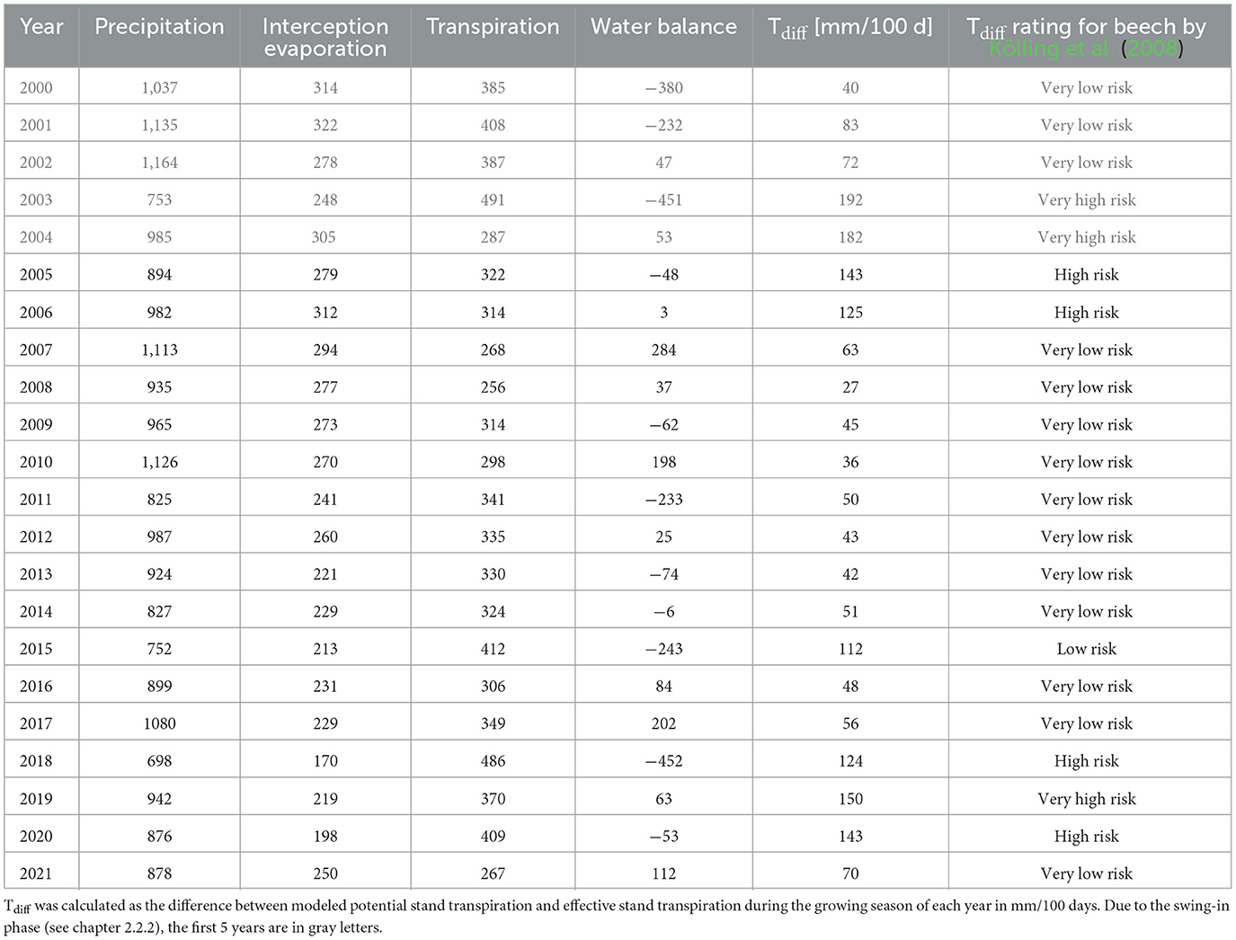
Table 1. Modeled parameters for the location of the forest monitoring plot supplemented by a classification of the transpiration difference T_diff according to Kölling et al. (2008).

3.1.1. Interception-evaporation

Yearly evaporated water after interception ranges between 100 mm and 450 mm for the forest areas (Figure 5). Crop and grasslands show distinctly lower interception compared to forested areas. Coniferous forests' interception evaporation is slightly higher than the modeled values of deciduous forest areas. Furthermore, interception evaporation is interannually decreasing with the lowest values in 2018.

FIGURE 5

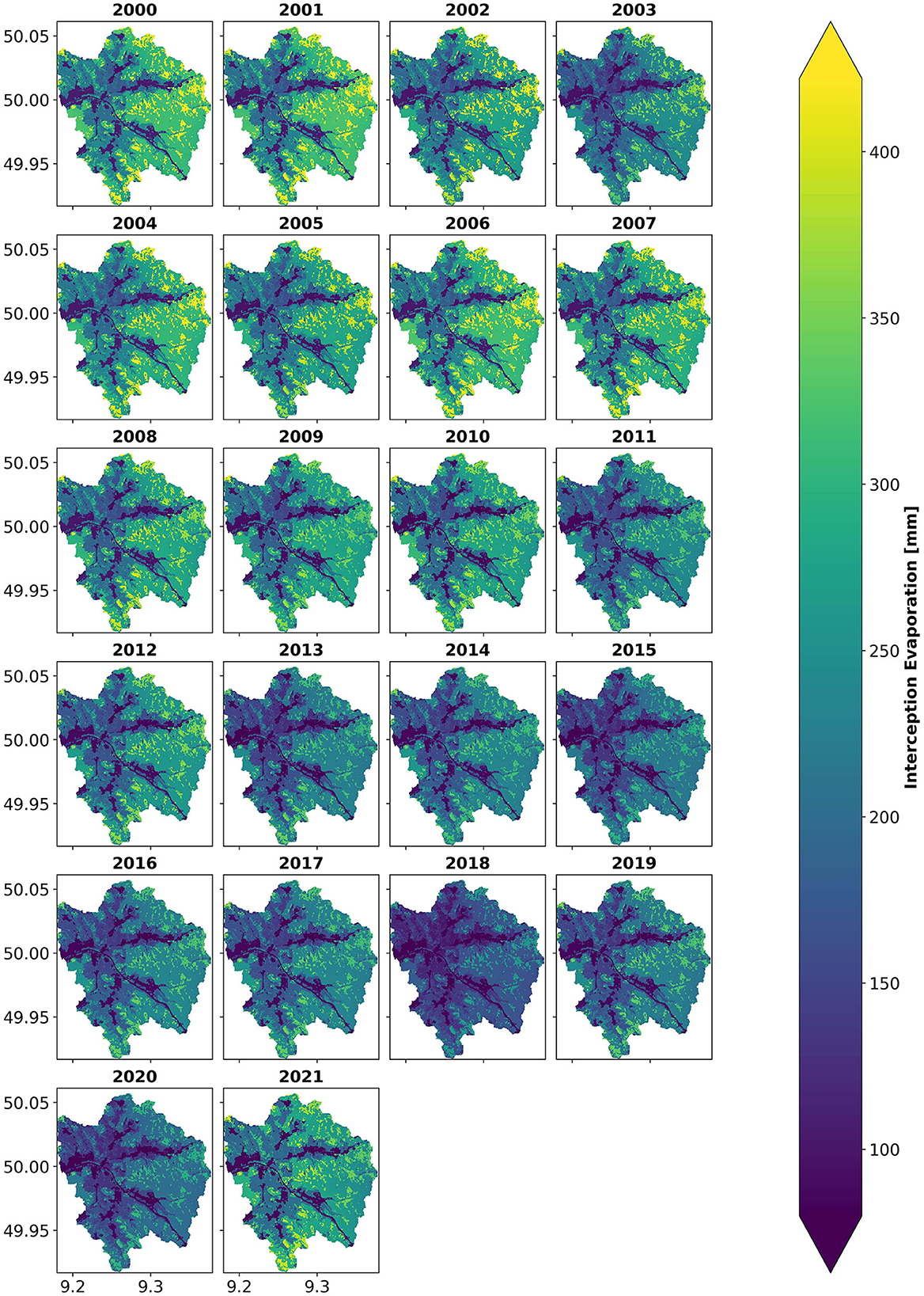
Figure 5. Spatial distribution of the yearly sums of interception evaporation from 2000 to 2021 in the surveyed catchment.

3.1.2. Forest stand transpiration

The 75% percentile of modeled forest pixels is in the range between 50 and 700 mm when considering annual sums of effective stand transpiration (Figures 6, 7). There are both spatial and temporal differences considering the modeled stand transpiration. The boxplots in Figure 7 illustrate the differences, with an obviously higher median of modeled transpiration rates in 2003, 2015, and 2018. Conversely, the transpiration median was at its lowest in 2021. Furthermore, there are many outliers with values between 50 and 200 mm throughout all years.

FIGURE 6

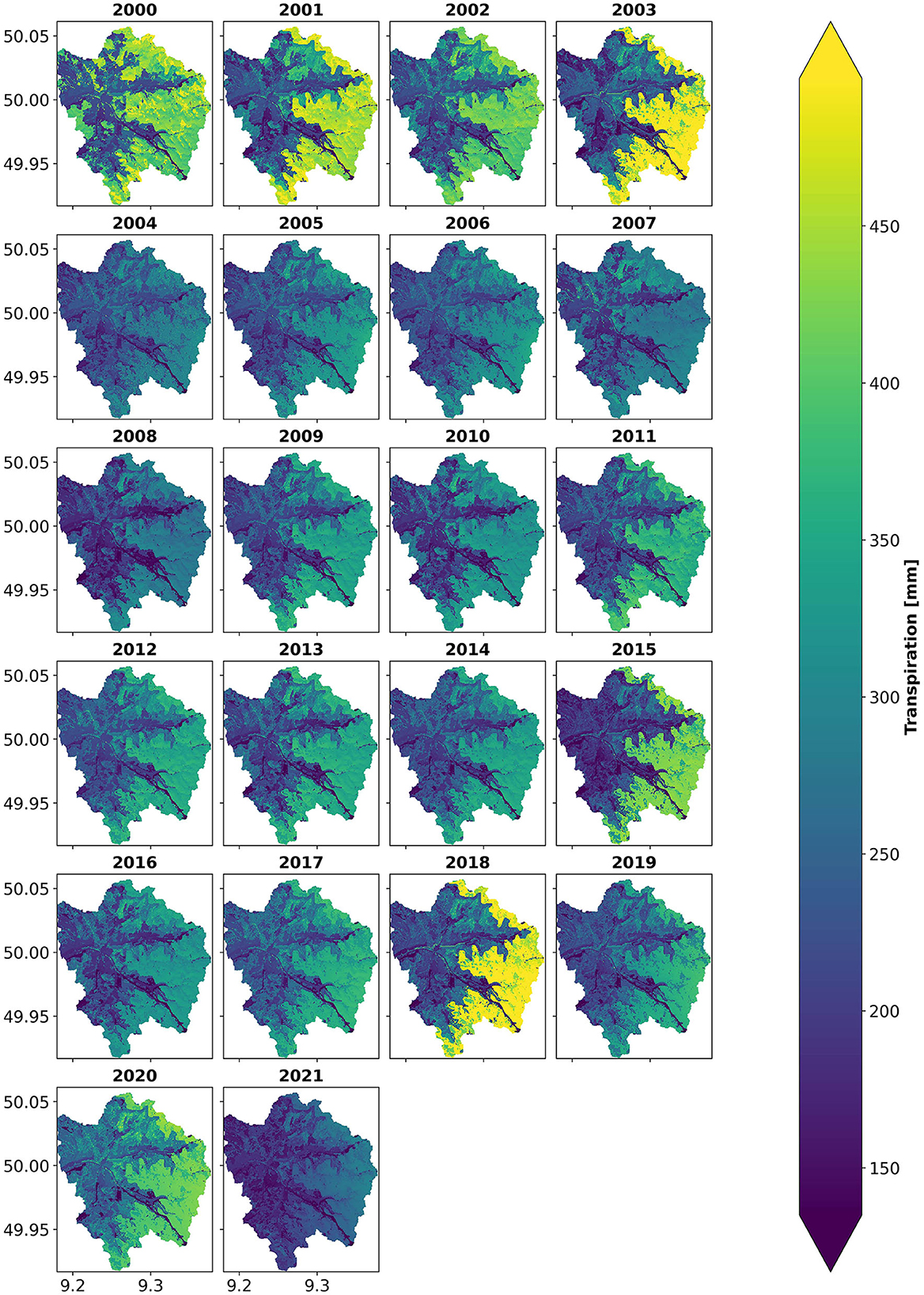
Figure 6. Spatial distribution of the yearly sums of effective transpiration from 2000 to 2021 in the surveyed catchment.

FIGURE 7

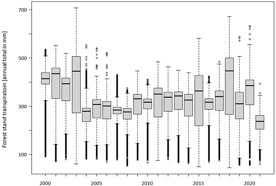
Figure 7. Boxplots with the annual sum of effective stand transpiration of the modeled forest pixels in the catchment.

3.1.3. Water balance and T_diff

The two calculated drought stress indicators for the forest monitoring plot pixels match with the dry and moist years (Table 1). T_diff, with values between 27 and 192 mm, is higher in 2003, 2004, 2005, 2006, 2015, 2018, 2019, and 2020 than in wetter years such as 2008, 2010, 2016, or 2017. The water balance estimation also highlights the above-mentioned dry and moist years with values between −452 and 284 mm, being the lowest in 2003 and 2018. The modeled values fit very well with the T_diff rating based on Kölling et al. (2008), consisting of four risk classes for beech cultivation. This vegetation-related drought stress indicator illustrates the long-term effects of single drought years, like 2003 or 2018.

3.2. Verification of the results

3.2.1. Runoff

The model setup shows a good representation of the observed runoff in each of the compiled time intervals from 2000 to 2021 (KGE ≥ 0.6; VE ≥ 0.5; R² ≥ 0.7). In this regard, yearly values deliver the best KGE (0.83) and VE (0.86), whereby the R² is very similar with a range of 0.7 to 0.8 in all temporal resolutions of observation. Besides these goodness-of-fit measures, Figure 8 further illustrates the temporal course of simulated and observed runoff for the watershed.

FIGURE 8

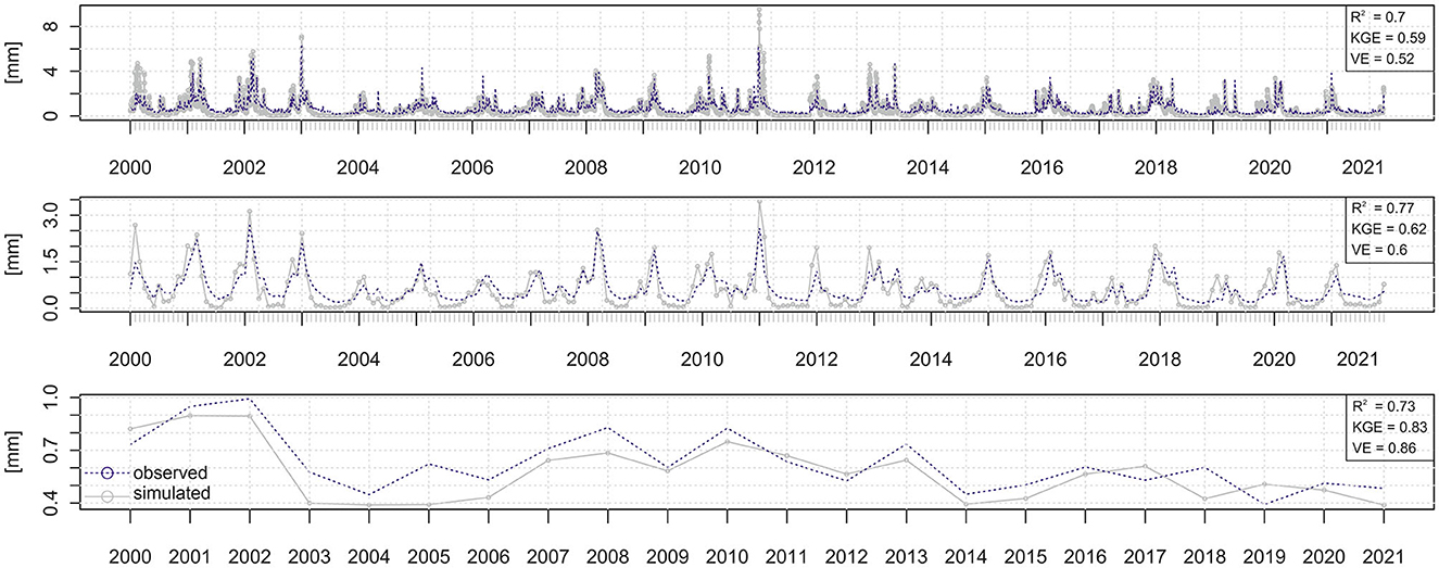
Figure 8. Time series of the modeled and observed runoff at the Aschaff River level gauge with daily (top), monthly (middle), and yearly (bottom) values.

3.2.2. Evapotranspiration

Figure 9 shows the correlation between the ET simulated by WaSiM-ETH and the calculated ET by MODIS data at the forest monitoring plot. As the MODIS dataset represents an 8-day composite of ET, the simulated outcomes were cumulated. Concerning these two ET values, the model outcome provides a stronger correlation (R² = 0.80) than the modeled runoff results (R² < 0.80; Figure 8).

FIGURE 9

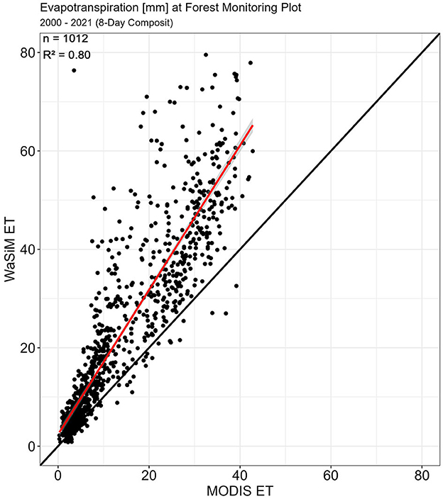
Figure 9. Correlation between the modeled evapotranspiration by WaSiM-ETH and the estimated evapotranspiration by MODIS data with a linear fit line (red) and a 1:1 line (black).

3.2.3. In situ data

The weather station in the forest monitoring plot (plus additional totalizers and stem flow measures) allows a comparison of the modeled and independently measured precipitation and interception for 2021. For both parameters, the simulated and in situ measured values are very similar, with a deviation of only 3.9% (simulated precipitation: 878 mm; observed precipitation: 845 mm) and 9.1% (simulated interception evaporation: 250 mm; observed interception evaporation: 229 mm), respectively. Owing to the installed TDR probes, a direct comparison of the modeled and observed mean volumetric water content in the main rooting zone is possible (Figure 10). Most conspicuous is the offset in the first half of the year (up to 7%) after starting at the same level in January 2021. In the second half, the seasonal development is very similar. Nevertheless, an R² of 0.55 and VE of 0.88 were achieved when correlating the daily measurements.

FIGURE 10

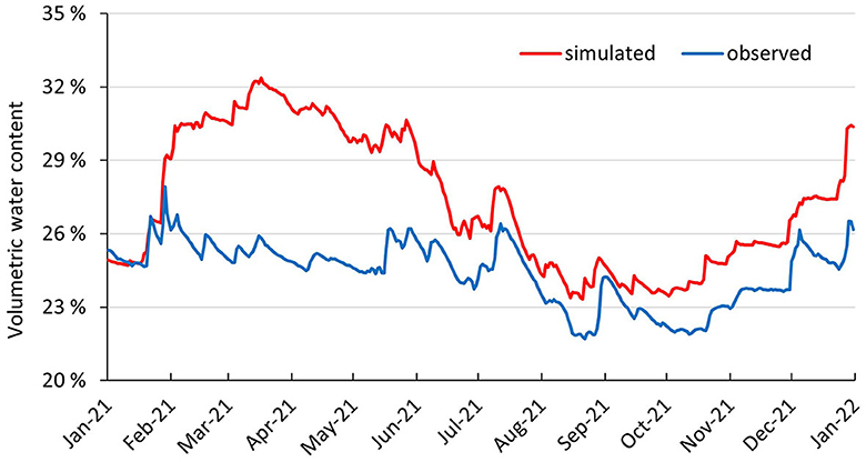
Figure 10. Time course of the simulated and observed volumetric water content in the main root zone of the forest monitoring plot in 2021.

4. Discussion

4.1. Key output parameters

4.1.1. Interception evaporation

The spatial differences of interception evaporation (Figure 5) mainly reflect the land use classes (Figure 4) entered as input and vary accordingly due to divergent land use-specific parameters. With a higher LAI (up to 10), the coniferous forests also differ significantly from the deciduous forests (LAI up to 8). This is because the LAI values (taken from Schulla, 2021b) on which this land use class is presumably derived from spruce stands, which is at least twice as high as, for example, pines (Mitscherlich, 1970; Gower and Norman, 1991). Therefore, pixels labeled as coniferous forests cannot be assigned to each conifer species, such as pine. Accordingly, in the future, a more detailed differentiation with respect to the main tree species of a stand must be made to prevent such overlaps. With distinctly lower values (Table 1), the interception evaporation also reflects the dry years (2003, 2015, and 2018) mentioned above and is in the order of magnitude with the value calculated out of the data observed at the monitoring plot for the year 2021 (9.1 % deviation).

4.1.2. Stand transpiration

Although the boxplots in Figure 7 only include forest pixels, there is a widespread of values. When considering the outliers with low values, these are found at the border of forested areas to croplands or grasslands. The values between 50 and 150 mm, described in Chapter 3.1.2, are in the range of typical values for grass or shrub cover (c.f. Klein, 2000; Gao et al., 2022). Overall, the median annual transpiration sums are in the order of magnitude for beech when comparing our findings with related results of Klein (2000). Considering the temporal component, the dry years 2003, 2015, and 2018 (Supplementary Figure 1) have a plausible impact with increased transpiration, as shown in Figure 7. The total 8-day sums of ET, modeled with WaSiM-ETH for the monitoring plot, show a good correlation with the values derived from MODIS data (Figure 9), despite the remote sensing product integrating over a 500-m raster. However, model outputs of WaSiM-ETH are generally higher than estimates of MODIS.

4.1.3. Water balance and T_diff

As one of the two calculated drought stress indicators, the annual water balance reflects the differently pronounced drought anomalies throughout the investigated period (Table 1). In contrast to interception evaporation, stand transpiration, and T_diff, the water balance in 2011 also appears relatively dry, which is probably due to the lower precipitation. The characteristics of the respective dry years can thus be well evaluated with the help of the water balance as a quantity integrating over several parameters. However, it should be noted that the years 2000–2005 are situated in the swing-in phase (see Chapter 2.2.2). This suggests the necessity of having a sufficiently long time series available.

The rather vegetation-related transpiration difference T_diff also shows the corresponding dry years but with small differences to the modeled water balance (Table 1). The range of modeled T_diff values also fits well on the range of cultivation risk classes for beech according to Kölling et al. (2008) as shown in Table 1. While T_diff describes the year 2011 as distinctly less critical than 2015, the modeled water balance is comparatively similar for both years. This is likely due to the higher temperatures in 2015 compared to 2011, having a higher influence on T_diff in relation to the water balance, which depends on more parameters. However, the interannual relations of both variables correspond to each other very well (Table 1) and can be seen as reliable and useful spatiotemporal drought indicators, directly derived from the WaSiM-ETH model output. The T_diff values, remaining low during and after years with a negative water balance (such as 2003 and 2018), indicate that tree transpiration rates are impacted for multiple years following extremely dry conditions. This underlines that these two indicators complement each other very well. Short-term variations in modeled water content, which is driven by water balance, are also largely consistent with water content measured in the main root zone of the forest monitoring plot (Figure 10).

4.2. Model limitations

4.2.1. Data basis

4.2.1.1. Meteorological data

As WaSiM-ETH is a strictly deterministic model, the quality of input parameters must be sufficient in terms of spatiotemporal resolution. Although there are clear advantages, such as the ability to generate many parameters relevant to hydro–ecological processes at almost any spatial resolution and time step, it is important to conduct a thorough and rigorous analysis of the input data for the model. This is necessary to ensure that the output datasets are reliable and have a high level of accuracy. For instance, the meteorological input of only one weather station would result in a different choice of spatial interpolation methods and an inaccurate reproduction of the meteorological conditions within the investigated area. In addition, it is essential that the time series data for each meteorological input parameter is complete and consistent for the entire simulation period. For our 21-year simulation, we found that using meteorological data from 21 DWD stations provided sufficient coverage.

4.2.1.2. Soil data

For a spatially high-resolution output with appropriate accuracy, a more accurate soil map and soil table should be pursued. The used soil map is rather coarse and integrates with respect to the soil properties over large areas, clearly exceeding the output resolution of 30 m. Nonetheless, the dataset provides grain size distributions on predominant soil types, considering soil depth, which is crucial for the estimation of the required Van Genuchten parameters. At least the soil type used at the forest monitoring plot location in the model was verified for grain size distribution and Van Genuchten Parameters based on soil analysis.

4.2.1.3. Land use/vegetation data

In this study, the data provided by Mack et al. (2016) were used as the basis for the different vegetation types with a resolution of 30 m. This map is displaying general land use types, as such does not provide well-differentiated information on forest stands. Considering the rather large catchment area (136 km²), we decided not to create a more detailed map. Nevertheless, future studies should incorporate more precise forest inventory maps, which at least allow differentiation by tree species or age instead of a division into coniferous and deciduous forests only. As indicated in Chapter 4.1, the LAI differs widely between coniferous tree species. The default LAI of up to 10 for coniferous forests (Schulla, 1997) presumably originates from values for spruce. However, pines, which also occur in this catchment, cannot be associated with such a high LAI (Mitscherlich, 1970; Gower and Norman, 1991), although they are assigned to it via the land use classes (Mack et al., 2016). A useful basis for a more accurate forest-specific land use map could be retrieved from the local forest management containing information on tree species composition, stand age, or form of management. Remote sensing products might also deliver information on tree species composition (Persson et al., 2018; Welle et al., 2022) and canopy structure (Kacic et al., 2023).

4.2.2. Model-specific limitations

The calibration step is usually the most time-consuming part of the modeling procedure. Although there are possibilities for semi- and autocalibration during the modeling process, a priori investigations of the area of interest is highly recommended, including the following important requirements:

• Available location of river level gauge(s) within the catchment.

• Accessible runoff data in a representative time span to derive Manning–Strickler parameter and specific runoff statistics.

• Accessible land use and soil maps containing hydrological soil parameters.

• Accessible meteorological data in respective resolution and format.

Model performance decreases with the lack of a suitable catchment-specific spatiotemporal setting, especially in lowland areas (Rieger, 2012). Additionally, the user manual provides chapters for parameter sensitivity analysis and calibration strategies (Schulla, 2021a). The simulated runoff continuum strongly depends on a linear scaling parameter for interflow, proper calibration of the soil module (i.e., number of layers, thickness, and hydrological parameters), and the interplay with the groundwater table. After a successful calibration process, the model outcome can contribute to future scenarios containing climate prospections. As WaSiM-ETH provides a vertical soil modeling approach with several numerical layers, interflow is calculated only if the soil layer holds suction <3.45 m (pF 2.5) or as a result of conductivity, river density, and hydraulic gradient (Schulla, 2021a). These limitations lead to the fact that lateral flows inside the soil section cannot be reproduced. However, as the amount of numerical layers is freely adjustable, this restriction can be minimized.

Considering the mentioned limitations above, our approach is not directly applicable to any location unless the mentioned prerequisites are fulfilled. The weaknesses of the database mentioned in Chapter 4.2.1 should be improved to directly derive forest management options for the future with the presented model. Owing to the high need for fine-scale assessments of water stress to support forest management during climate change (Field et al., 2020), the parameterized model of this study nevertheless provides a valuable first approach.

4.2.3. Verification

4.2.3.1. Runoff

The calibration process within WaSiM-ETH relies on measured discharge data. However, due to artificial drainage in urban areas (red cells in Figure 4), as well as water evacuation from springs, bordered in forests, the natural runoff behavior is altered considerably. Nevertheless, this study replicates a simulated runoff behavior without the consideration of human impact. Furthermore, as the simulation was conducted on a spatial resolution of 30 m per cell with daily timesteps, the impacts of certain meteorological events (e.g., short and heavy rainfalls and storms) are therefore discretized in time and space. This may lead to an unbalanced volume efficiency.

4.2.3.2. Evapotranspiration

Compared to our hydrological simulation, MODIS ET provides a coarse spatiotemporal resolution of 500 m and an acquisition period of 8 days. The spatial discrepancy between a high-resolution output of the hydrological model and a satellite-based remote sensing product can be perceived as critical unless the occurrence of the investigated land use pattern of the monitoring plot is mostly represented within the larger pixel size. Figure 11 illustrates the spatial offset of nine MODIS pixels compared to the land use pattern distribution, as configurated in the model. Owing to the Landsat-derived landcover product, almost every pixel in the MODIS dataset (containing the monitoring plot) is declared as broadleaf woodland, as well as the adjacent area. Due to MODIS optical sensor equipment, the ET product MOD16A2GFv006 was generated using a backup algorithm if a high level of cloud coverage is present. As stated by Running et al. (2019), ET is underestimated over areas with frequent cloudiness which could be the reason for the offset of ET in Figure 9. However, because ET calculation in MODIS and WaSiM-ETH follow the logic of Penman–Monteith, the generated results should be comparable.

FIGURE 11

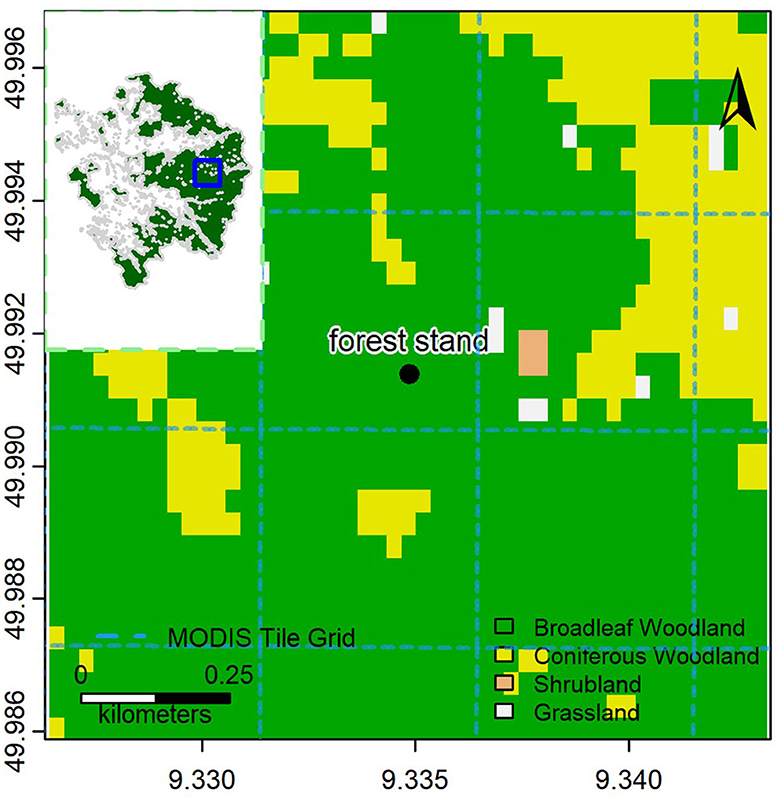
Figure 11. Comparative illustration of the different resolutions of the hydrological modeling with WaSiM-ETH (shown by the land use classes) and the evapotranspiration calculated from MODIS data (light blue frames).

4.2.3.3. In situ data

Despite the advantages of comparing the modeled output with observed in situ data, only one full year (2021) of data was available. Therefore, not the entire modeling period could be verified by in situ data. Considering the offset of ET between MODIS and WaSiM-ETH (Figure 9), it would be of interest to see whether precipitation and interception sums also match in previous years. Therefore, the longest possible in situ time series should be used for the verification of hydrological modeling outputs.

Regarding the offsets in the first half of the year from the modeled and in situ measured water content in the root zone, the very coarse-scale soil map of the BGR may be one reason. This map aggregates over wide-ranging areas for the data on grain size distribution and has for instance a lower sand content than measured at the forest monitoring plot. This could also be one reason for the partly higher modeled effective ET compared to the values out of MODIS (Figure 9), which is due to a higher field capacity in the hydrological model. The offset in water content could be further driven by the measurement error of the ECH₂O probes themselves (±3% according to the manufacturer).

4.3. Model advantages

We showed that WaSiM-ETH is a potential hydrological model for investigating water balance and (evapo-)transpiration on forest stands additionally using MODIS remote sensing datasets for verification. Due to new modern methods from remote sensing, numerous 2-dimensional raster data are available today that are well suited as input data for WaSiM-ETH. These are, for example, land use (like Landsat-derived landcover products, e.g., GWELDYRv031; Roy and Zhang, 2019) or soil maps (BUEK200; BGR, 2020), which are freely available. Because of the constantly evolving data quality of remote sensing products, it is possible to adapt multidimensional raster data to WaSiM-ETH to gain new insights on catchment hydrology as well as climate change impacts on corresponding forest ecosystems. As additional help for forest management, plausible forest-specific indices were derived and applied to phenological observations. One example is the calculation of T_diff, which requires both spatially and temporally resolved phenological data, such as the beginning and end of the growing season. These could be obtained as raster data from the DWD and interpolated into the model grid resolution of 30 m. The result is a spatial distribution of the yearly beginning and end of the growing season for the forest pixels (Figure 12).

FIGURE 12

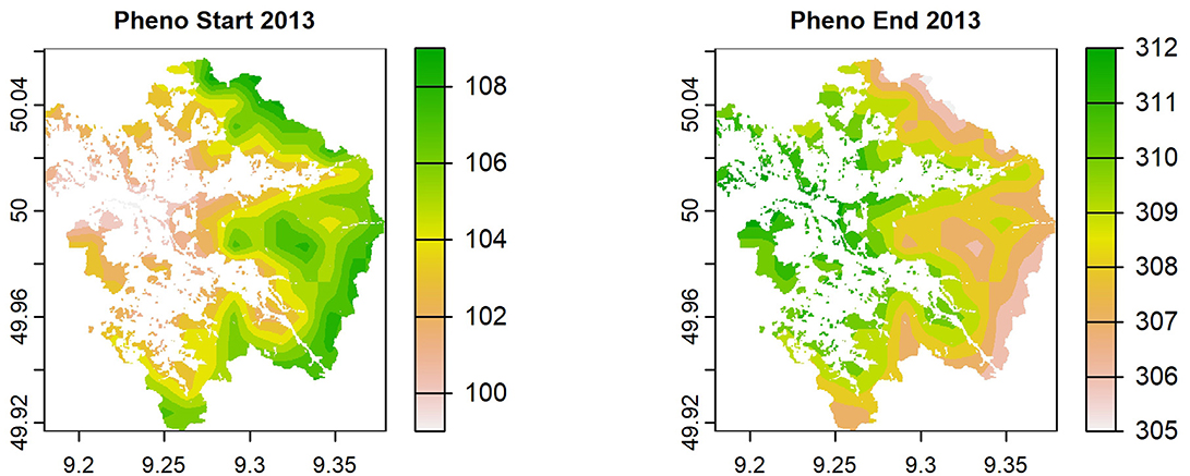
Figure 12. Raster layer containing Julian Day with the beginning (left) and the end (right) of the growing season in 2013 within the modeled catchment. Phenological data were derived from DWD.

Due to the spatial component, different possibilities are feasible in addition to the comparison of individual pixels with in situ data, such as calibrating the model by comparing the total runoff with a river level gauge. Moreover, the multidimensional features of WaSiM-ETH allow a comparison of the modeled water balance outputs with remote sensing data. This is important because MODIS data provide the ET, also calculated by using the Penman–Monteith equation. The usage of multiple verification approaches was very helpful during the calibration phase. Owing to the high complexity and the resulting high calibration effort, facilitation and acceleration of the calibration with the help of such methods are of great importance.

4.4. Outlook

As mentioned in Chapter 4.2.1, the model limitations are mainly driven by the data basis implemented in WaSiM-ETH. Therefore, raster input data should not only be featured by a high resolution but also by a realistic spatial differentiation of the underlying values. This is especially true for land use as well as soil input. For further investigations, new interpolation methods can be developed to describe in-depth (forest-)soil hydrology by a combination of state-of-the-art land use and soil maps, observations, and advanced pedotransfer functions. For example, there exist several approaches to increase the spatial resolution, like Random Forests or Neural Networks (Taghizadeh-Mehrjardi et al., 2020; Kobs et al., 2021) that could also be applied to other regions. A more differentiated land use map, e.g., by tree species, would also be possible according to the current state of knowledge in remote sensing and should be prepared for future modeling. In this study, the Dynamic Phenology Module (DPM) of WaSiM-ETH was not used. However, to model interannual forest stand dynamics more accurately, a combination of DPM with other forest growth simulators like SILVA 2.0 (Pretzsch et al., 2002) could be utilized. This would allow the inclusion of year-dependent tree age and tree dimensions to estimate and recalibrate sensitive spatiotemporal specific parameters (e.g., LAI, minimum surface resistance, root density distribution, root depth, stomata resistance; also see Sutmöller et al., 2007). The model interface can process gridded meteorological input data in a NetCDF file format, which is a standard format for many regional and global climate models (CM). Thus, there is a possibility for investigating climate change scenarios either by pre-defined deviation tables or using bias-corrected CM outputs directly.

Especially on low land catchments, groundwater interaction plays an important role in water balance and runoff generation. Although WaSiM-ETH provides a groundwater simulation module, lateral fluxes as well as primary geological groundwater formations cannot be depicted. This task can be outsourced to a more complex model using the “External Coupling” module. One example is given by Krause et al. (2007) coupling WaSiM-ETH with USGS Modflow (Harbaugh, 2005).

To finally offer spatially high-resolution and reliable tree species recommendations for forest management based on WaSiM-ETH, the nutrient supply is also a very important variable in addition to physical influencing variables (Mellert and Ewald, 2014; Mellert et al., 2018). Therefore, the possibility to adapt the surface routing model for tracers to monitor nutrient flow inside the catchment should be examined. If this is possible, an attempt could be made to include nutrient supply, also for long-term climate forecasts.

5. Conclusion

To the best of our knowledge, this is the first study modeling the water balance within a forested catchment with WaSiM-ETH by calibrating and verifying the model using a comprehensive combination of methods using in situ data, the MODIS Evapotranspiration product (MOD16A2GFv006) and total runoff. The modeled effective (ET) correlates very well with the estimated ET (R² = 0.80) of MODIS. Depending on daily (R²= 0.70; KGE = 0.59; VE = 0.52), monthly (R² = 0.77; KGE = 0.62; VE = 0.60), or yearly (R² = 0.73; KGE = 0.83; VE = 0.86) values, there is also a good match between simulated and observed runoff. The comparison with in situ data from a forest monitoring plot, established at the end of 2020, also provides good matches considering precipitation, interception, and soil water content. The two modeled drought stress indicators (water balance and T_diff) also fit well to dry years as annual sums.

Although there are some model limitations, especially considering the data basis, WaSiM-ETH offers great potential, also for forest management, owing to its multidimensionality. The outputs deliver spatial differentiability, which is very important in forestry due to small-scale varying variables such as stand structure and soil properties. Due to the spatial component, additional verification possibilities are feasible, such as evaluating the total runoff by a river level gauge that integrates over the entire modeled catchment. This also allows a comparison of the modeled water balance outputs with remote sensing data. Due to large uncertainties regarding the outputs of hydrological models, every additional verification possibility should be used to generate realistic parameterizations and thus robust models for reliable future forecasts. Especially for future projections, models that are as robust as possible are indispensable as there is no possibility of verification for these results. Therefore, multidimensional hydrological models, such as WaSiM-ETH, should receive more attention, especially in forestry, although the model presented in this study needs further improvement before forest management options for the future can be directly derived for practice.

Nevertheless, the parameterized model of this study offers a valuable first approach, as the entire hydrological catchment with its surface and subsurface conditions must be considered for forestry issues, especially in times of climate change.

Data availability statement

The original contributions presented in the study are included in the article/Supplementary material, further inquiries can be directed to the corresponding author.

Author contributions

Conceptualization, methodology, investigation, data curation, and review and editing: CS, JF, TU, and CK. Software, validation, original draft preparation, and visualization: CS and JF. Resources, project administration, and funding acquisition: CK and RB. Supervision: TU, CK, and RB. All authors have read and agreed to the published version of the manuscript.

Funding

The study was funded by the European Regional Development Fund (ERDF) (BigData@Geo; grant number 20-3044-2-11) as well as by the German Federal Ministry of Food and Agriculture and the German Federal Ministry for the Environment, Nature Conservation, Nuclear Safety, and Consumer Protection (BodenWasserWald; grant number 2218WK22X1). This publication was supported by the Open Access Publication Fund of the University of Würzburg.

Acknowledgments

We are grateful for the provision of runoff data, delivered by the BEA. We further thank Mack et al. for providing the land use and land cover product.

Conflict of interest

The authors declare that the research was conducted in the absence of any commercial or financial relationships that could be construed as a potential conflict of interest.

Publisher's note

All claims expressed in this article are solely those of the authors and do not necessarily represent those of their affiliated organizations, or those of the publisher, the editors and the reviewers. Any product that may be evaluated in this article, or claim that may be made by its manufacturer, is not guaranteed or endorsed by the publisher.

Supplementary material

The Supplementary Material for this article can be found online at: https://www.frontiersin.org/articles/10.3389/ffgc.2023.1186304/full#supplementary-material

References

Airbus (2020). Copernicus DEM: Copernicus Digital Elevation Model Product Handbook (RFP/RFI-No. AO/1-9422/18/I-LG, Version 3.0). Available onliine at: https://spacedata.copernicus.eu/documents/20126/0/GEO1988-CopernicusDEM-SPE-002_ProductHandbook_I3.0+%281%29.pdf/68854203-e022-1446-b216-41becd2399b5?t=1618937501277 (accessed August 8, 2022).

Google Scholar

Allen, C. D., Macalady, A. K., Chenchouni, H., Bachelet, D., McDowell, N., Vennetier, M., et al. (2010). A global overview of drought and heat-induced tree mortality reveals emerging climate change risks for forests. For. Ecol. Manag. 259, 660–684. doi: 10.1016/j.foreco.2009.09.001

CrossRef Full Text | Google Scholar

Arnold, J. G., Srinivasan, R., Muttiah, R. S., and Williams, J. R. (1998). Large area hydrologic modeling and assessment part I: model development 1. J. Am. Water Res. Assoc. 34, 73–89. doi: 10.1111/j.1752-1688.1998.tb05961.x

CrossRef Full Text | Google Scholar

Ashby, S. F., and Falgout, R. D. (1996). A parallel multigrid preconditioned conjugate gradient algorithm for groundwater flow simulations. Nuclear Sci Engi. 124, 145–159. doi: 10.13182/NSE96-A24230

CrossRef Full Text | Google Scholar

BEA (2022). “Gewässerkundlicher Dienst Bayern,” in Bavarian Environment Agency. Available onliine at: https://www.gkd.bayern.de (accessed July 1, 2022).

Beckers, J., Pike, R., Werner, A. T., Redding, T., Smerdon, B., and Anderson, A. (2009b). Hydrologic models for forest management applications: Part 2: Incorporating the effects of climate change. Watershed Manag. Bullet. 13, 45–54.

Google Scholar

Beckers, J., Smerdon, B., Redding, T., Anderson, A., Pike, R., and Werner, A. (2009a). Hydrologic models for forest management applications: part 1: model selection. Streamline Watershed Manag. Bullet. 13, 35–44.

Google Scholar

BGR (2020). Bodenübersichtskarte 1:200.000 (BÜK200). Available onliine at: https://www.bgr.bund.de/DE/Themen/Boden/Informationsgrundlagen/Bodenkundliche_Karten_Datenbanken/BUEK200/buek200_node.html (accessed May 1, 2020).

Google Scholar

Cholet, C., Houle, D., Sylvain, J. D., Doyon, F., and Maheu, A. (2022). Climate change increases the severity and duration of soil water stress in the temperate forest of eastern North America. Front. Forests Global Chang. 5, 879382. doi: 10.3389/ffgc.2022.879382

CrossRef Full Text | Google Scholar

Criss, R. E., and Winston, W. E. (2008). Do Nash values have value? Discussion and alternate proposals. Hydrol.Proc. 22, 2723–2725. doi: 10.1002/hyp.7072

CrossRef Full Text | Google Scholar

DWD (2021). Vieljährige Mittelwerte. Deutscher Wetterdienst. Available onliine at: https://www.dwd.de/DE/leistungen/klimadatendeutschland/vielj_mittelwerte.html (accessed October 28, 2021).

Google Scholar

DWD (2022). Daily Climate observation data for Germany. Available onliine at: https://opendata.dwd.de/climate_environment/CDC/observations_germany/climate/daily/kl/recent/ (accessed July 1, 2022).

Google Scholar

Etzold, S., Waldner, P., Thimonier, A., Schmitt, M., and Dobbertin, M. (2014). Tree growth in Swiss forests between 1995 and 2010 in relation to climate and stand conditions: recent disturbances matter. Forest Ecology Manag. 311, 41–55. doi: 10.1016/j.foreco.2013.05.040

CrossRef Full Text | Google Scholar

Falk, W., Dietz, E., Grünert, S., Schultze, B., and Kölling, C. (2008). Wo hat die Fichte genügend Wasser? LWF Aktuell. 66, 21–25.

Google Scholar

Field, J. P., Breshears, D. D., Bradford, J. B., Law, D. J., Feng, X., and Allen, C. D. (2020). Forest management under megadrought: urgent needs at finer scale and higher intensity. Front. For. Glob. Change. 3, 502669. doi: 10.3389/ffgc.2020.502669

CrossRef Full Text | Google Scholar

Fischer, S., Keupp, L., Paeth, H., Göhlich, M., and Schmitt, J. (2022). Climate adaptation as organizational learning: a grounded theory study on manufacturing companies in a Bavarian Region. Educ. Sci. 12, 22. doi: 10.3390/educsci12010022

CrossRef Full Text | Google Scholar

Förster, K., Garvelmann, J., Meißl, G., and Strasser, U. (2018). Modelling forest snow processes with a new version of WaSiM. Hydrol Sci J. 63, 1540–1557. doi: 10.1080/02626667.2018.1518626

CrossRef Full Text | Google Scholar

Gao, G., Wang, D., Zha, T., Wang, L., and Fu, B. (2022). A global synthesis of transpiration rate and evapotranspiration partitioning in the shrub ecosystems. J. Hydrol. 606, 127417. doi: 10.1016/j.jhydrol.2021.127417

CrossRef Full Text | Google Scholar

Gower, S. T., and Norman, J. M. (1991). Rapid estimation of leaf area index in conifer and broad-leaf plantations. Ecology. 72, 1896–1900. doi: 10.2307/1940988

CrossRef Full Text | Google Scholar

Grigoryan, G. V., Casper, M. C., Gauer, J., Vasconcelos, A. C., and Reiter, P. P. (2010). Impact of climate change on water balance of forest sites in Rhineland-Palatinate, Germany. Adv. Geosci. 27, 37–43. doi: 10.5194/adgeo-27-37-2010

CrossRef Full Text | Google Scholar

Gupta, H. V., Kling, H., Yilmaz, K. K., and Martinez, G. F. (2009). Decomposition of the mean squared error and NSE performance criteria: Implications for improving hydrological modelling. J. Hydrol. 377, 80–91. doi: 10.1016/j.jhydrol.2009.08.003

CrossRef Full Text | Google Scholar

Hamman, J. J., Nijssen, B., Bohn, T. J., Gergel, D. R., and Mao, Y. (2018). The Variable Infiltration Capacity model version 5 (VIC-5): Infrastructure improvements for new applications and reproducibility. Geosci. Model Dev. 11, 3481–3496. doi: 10.5194/gmd-11-3481-2018

CrossRef Full Text | Google Scholar

Hammel, K., and Kennel, M. (2001). “Charakterisierung und Analyse der Wasserverfügbarkeit und des Wasserhaushalts von Waldstandorten in Bayern mit dem Simulationsmodell BROOK90,” in Forstliche Forschungsberichte München. (Freising: Zentrum Wald-Forst-Holz Weihenstephan), p. 185

Harbaugh, A. W. (2005). MODFLOW-2005, the US Geological Survey Modular Ground-Water Model: the Ground-Water Flow Process (Vol. 6). Reston, VA, USA: US Department of the Interior, US Geological Survey.

Google Scholar

Jasper, K., Calanca, P., and Fuhrer, J. (2006). Changes in summertime soil water patterns in complex terrain due to climatic change. J. Hydrol. 327, 550–563. doi: 10.1016/j.jhydrol.2005.11.061

CrossRef Full Text | Google Scholar

Kacic, P., Thonfeld, F., Gessner, U., and Kuenzer, C. (2023). Forest structure characterization in Germany: novel products and analysis based on GEDI, sentinel-1 and sentinel-2 data. Remote Sens. 15, 1969. doi: 10.3390/rs15081969

CrossRef Full Text | Google Scholar

Kasei, R. A. (2010). Modelling Impacts of Climate Change on Water Resources in the Volta Basin. [dissertation]. Universitäts-und Landesbibliothek Bonn, Rheinische Friedrich-Wilhelms-Universität Bonn.

PubMed Abstract | Google Scholar

Kassa, A. K. (2013). Downscaling Climate Model Outputs for Estimating the Impact of Climate Change on Water Availability over the Baro-Akobo River Basin, Ethiopia. [dissertation]. Universitäts-und Landesbibliothek Bonn: Rheinische Friedrich-Wilhelms-Universität Bonn.

Google Scholar

Klein, M. (2000). Langjaähriger Wasserhaushalt von Gras-und Waldbeständen: Entwicklung, Kalibrierung und Anwendung des Modells LYFE am Groß-Lysimeter St. Arnold (Doctoral dissertation). Universität Osnabrück, Osnabrück, Germany.

Google Scholar

Kling, H., Fuchs, M., and Paulin, M. (2012). Runoff conditions in the upper Danube basin under an ensemble of climate change scenarios. J. Hydrol. 424–425, 264–277. doi: 10.1016/j.jhydrol.2012.01.011

CrossRef Full Text | Google Scholar

Kobs, K., Schäfer, C., Steininger, M., Krause, A., Baumhauer, R., Paeth, H., and Hotho, A. (2021). Semi-Supervised Learning for Grain Size Distribution Interpolation. Cham: Springer International Publishing. p. 34–44.

Google Scholar

Kölling, C., Bachmann, M., Falk, W., Grünert, S., and Wilhelm, G. (2008). Soforthilfe Baumarteneignung-Anbaurisiko-Klimawandel. LWF–Bayerische Landesanstalt für Wald und Forstwirtschaft–Technischer Report. Freising. Available online at: https://www.afsv.de/images/download/arbeitsgruppe/2009_01_27_SOFORTHILFE_Technical%20Report.pdf (accessed March 12, 2023).

Krause, S., Jacobs, J., and Bronstert, A. (2007). Modelling the impacts of land-use and drainage density on the water balance of a lowland–floodplain landscape in northeast Germany. Ecol. Model. 200, 475–492. doi: 10.1016/j.ecolmodel.2006.08.015

CrossRef Full Text | Google Scholar

LDBV (2021). Digitales Geländemodell 25m. Landesamt für Digitalisierung, Breitband und Vermessung.

Liang, X., Lettenmaier, D. P., Wood, E. F., and Burges, S. J. (1994). A simple hydrologically based model of land surface water and energy fluxes for general circulation models. J. Geophysical Res. 99, 14415–14428. doi: 10.1029/94JD00483

CrossRef Full Text | Google Scholar

Lindsay, J. (2014). The Whitebox Geospatial Analysis Tools project and open-access GIS. Glasgow, UK: GIS Research UK 22nd Annual Conference.

Google Scholar

Mack, B., Leinenkugel, P., Kuenzer, C., and Dech, S. (2016). A semi-automated approach for the generation of a new land use and land cover product for Germany based on Landsat time-series and Lucas in-situ data. Remote Sens. Lett. 8, 244–253. doi: 10.1080/2150704X.2016.1249299

CrossRef Full Text | Google Scholar

Mellert, K. H., and Ewald, J. (2014). Nutrient limitation and site-related growth potential of Norway spruce (Picea abies [L.] Karst) in the Bavarian Alps. Eur. J. Forest Res. 133, 433–451. doi: 10.1007/s10342-013-0775-1

CrossRef Full Text | Google Scholar

Mellert, K. H., Lenoir, J., Winter, S., Kölling, C., Carni, A., Dorado-Linan, I., et al. (2018). Soil water storage appears to compensate for climatic aridity at the xeric margin of European tree species distribution. Eur. J. Forest Res. 137, 79–92. doi: 10.1007/s10342-017-1092-x

CrossRef Full Text | Google Scholar

Mitscherlich, G. (1970). Form und Wachstum von Baum und Bestand, Bd 1 (Wald, Wachstum und Umwelt - Eine Einfuhrung in die okologischen Grundlagen des Waldwachstums). Frankfurt am Main:Sauerländer's Verlag.

Moore, R. D., Hutchinson, D. G., and Weiler, W. (2007). “Predicting the effects of post-MPB salvage harvesting using a conceptual streamflow model (HBV-EC): Initial evaluation using a paired-catchment approach,” in Mountain pine beetle and watershed hydrology workshop: Preliminary results of research from BC, Alberta and Colorado. Kelowna, BC: Ramada Inn. p. 41–42.

Google Scholar

Penman, H. (1978). Vegetation and the Atmosphere. Monteith, J. L. (ed). London: Academic Press. (1975). p. 459.

Google Scholar

Persson, M., Lindberg, E., and Reese, H. (2018). Tree species classification with multi-temporal Sentinel-2 data. Remote Sens. 10, 1794. doi: 10.3390/rs10111794

CrossRef Full Text | Google Scholar

Pretzsch, H., Biber, P., and Durský, J. (2002). The single tree-based stand simulator SILVA: construction, application and evaluation. Forest Ecol. Manag. 162, 3–21. doi: 10.1016/S0378-1127(02)00047-6

CrossRef Full Text | Google Scholar

Richards, L. A. (1931). Capillary conduction of liquids through porous mediums. Physics. 1, 318–333. doi: 10.1063/1.1745010

CrossRef Full Text | Google Scholar

Rieger, W. (2012). Prozessorientierte Modellierung dezentraler Hochwasserschutzmaßnahmen. [dissertation]. Munich: Universität der Bundeswehr München.

Roy, D., and Zhang, H. (2019). “NASA Global Web-Enabled Landsat Data Annual Global 30 m V031 [Data set],” in NASA EOSDIS Land Processes DAAC. (Washington, DC: National Aeronautics and Space Administration).

Running, S., Mu, Q., and Zhao, M. (2021). “MODIS/Terra Net Evapotranspiration 8-Day L4 Global 500m SIN Grid V061,” in NASA EOSDIS Land Processes DAAC (Washington, DC: National Aeronautics and Space Administration).

Running, S. W., Mu, Q., Zhao, M., and Moreno, A. (2019). MODIS global terrestrial evapotranspiration (ET) product (MOD16A2/A3 and year-end gap-filled MOD16A2GF/A3GF) NASA Earth Observing System MODIS Land Algorithm (for collection 6). Washington, DC, USA: National Aeronautics and Space Administration.

Google Scholar

Samaniego, L., Kumar, R., and Attinger, S. (2010). Multiscale parameter regionalization of a grid-based hydrologic model at the mesoscale. Water Res. Res. 46, 5. doi: 10.1029/2008WR007327

CrossRef Full Text | Google Scholar

Schuldt, B., Buras, A., Arend, M., Vitasse, Y., Beierkuhnlein, C., Damm, A., et al. (2020). A first assessment of the impact of the extreme 2018 summer drought on Central European forests. Basic Appl Ecol. 45, 86–103. doi: 10.1016/j.baae.2020.04.003

CrossRef Full Text | Google Scholar

Schulla, J. (1997). Hydrologische Modellierung von Flussgebieten zur Abschätzung der Folgen von Klimaänderungen. Zürich: ETH Zürich.

Schulla, J. (2021a). Model Description WaSiM. Technical Report. Available online at: http://wasim.ch/downloads/doku/wasim/wasim_2021_en.pdf (accessed July 25, 2022).

Schulla, J. (2021b). WaSiM (Richards). Available online at: http://wasim.ch/de/products/wasim_richards.htm (accessed July 25, 2022).

Schultze, B., Kölling, C., Dittmar, C., Rötzer, T., and Elling, W. (2005). Konzept für ein neues quantitatives Verfahren zur Kennzeichnung des Wasserhaushaltes von Waldböden in Bayern: Modellierung–Regression–Regionalisierung. Forstarchiv. 76, 155–163.

Šimůnek, J., and van Genuchten, M. T. (2008). Modeling nonequilibrium flow and transport processes using HYDRUS. Vadose Zone J. 7, 782–797. doi: 10.2136/vzj2007.0074

CrossRef Full Text | Google Scholar

Sutmöller, J., Hentschel, S., Meesenburg, H., and Spellmann, H. (2007). “Auswirkungen forstlicher Maßnahmen auf den Wasserhaushalt in bewaldeten Einzugsgebieten,” in Einfluss von Bewirtschaftung und Klima auf Wasser-und Stoffhaushalt von Gewässern, Miegel, K., Trübner, E.-R. u. Kleeberg, H.-B. (eds.). Beiträge zum Tag der Hydrologie 235–246.

Google Scholar

Taghizadeh-Mehrjardi, R., Mahdianpari, M., Mohammadimanesh, F., Behrens, T., Toomanian, N., Scholten, T., et al. (2020). Multi-task convolutional neural networks outperformed random forest for mapping soil particle size fractions in central Iran. Geoderma. 376, 114552. doi: 10.1016/j.geoderma.2020.114552

CrossRef Full Text | Google Scholar

Van Genuchten, M. T. (1980). A closed-form equation for predicting the hydraulic conductivity of unsaturated soils. Soil Sci. Soc. Am. J. 44, 892–898. doi: 10.2136/sssaj1980.03615995004400050002x

PubMed Abstract | CrossRef Full Text | Google Scholar

Welle, T., Aschenbrenner, L., Kuonath, K., Kirmaier, S., and Franke, J. (2022). Mapping dominant tree species of german forests. Remote Sens. 14, 3330. doi: 10.3390/rs14143330

PubMed Abstract | CrossRef Full Text | Google Scholar

Whitaker, A., Alila, Y., Beckers, J., and Toews, D. (2002). Evaluating peak flow sensitivity to clear-cutting in different elevation bands of a snowmelt-dominated mountainous catchment. Water Resour. Res. 38, 1172. doi: 10.1029/2001WR000514

CrossRef Full Text

Zhang, Y., Schaap, M. G., and Zha, Y. (2018). A high-resolution global map of soil hydraulic properties produced by a hierarchical parameterization of a physically based water retention model, Water Resour. Res. 54, 9774–9790. doi: 10.1029/2018WR023539

CrossRef Full Text | Google Scholar

Zhao, F., Wu, Y., Yin, X., Alexandrov, G., and Qiu, L. (2022). Toward sustainable revegetation in the Loess Plateau using coupled water and carbon management. Engineering. 15, 143–153. doi: 10.1016/j.eng.2020.12.017

CrossRef Full Text | Google Scholar