Optimization of tropical rainforest ecosystem management: implications from the responses of ecosystem service values to landscape pattern changes in Hainan Tropical Rainforest National Park, China, over the past 40 years

1. Introduction

The concept of ecosystem service (ES) was first introduced in the report “Man’s Impact on the Global Environment,” published by the United Nations University (UNU) in the early 1970s. The introduction of this concept built a bridge between ecosystems and humans, emphasizing the importance of ecosystems to human welfare (Schröter et al., 2019). The welfare of humans depends on tangible services (such as food, medicines, and raw materials) and intangible services (such as ecotourism, aesthetic beauty, cultural landscapes, climate regulation, and flooding resistance) provided by forests, wetlands, and other ecological systems to maintain and guarantee (Ayensu et al., 1999; Kemkes et al., 2010; Hernández-Morcillo et al., 2013). The Millennium Ecosystem Assessment (MA) (Millennium Ecosystem Assessment, 2005) defined the ESs as the benefits humans derive from ecosystems and classified them into four categories: provisioning services, regulating services, supporting services, and cultural services. For human societies to fully recognize these ESs, the ecosystem service values (ESVs) accounting is gradually becoming an effective way to understand ecosystems’ multiple benefits (Guo et al., 2001). Costanza et al. (1997) have also pointed out that ESs monetization can help increase policymakers’ attention to ESs. While this approach to assigning economic values to ESs has raised questions and concerns among some scholars (Fairhead et al., 2012), it is undeniable that the approach of quantifying ESs in the form of a common currency has allowed people to weigh the relative importance of ESs against other services, and the importance of ESs was enhanced (Tallis and Kareiva, 2005; De Groot et al., 2012; Guswa et al., 2014). With the gradual development of relevant studies on ESVs (Kroeger and Casey, 2007; Campbell and Tilley, 2014; Salzman et al., 2018), the concept of ES has also been further improved and promoted.

The landscape pattern is a mixture of natural and human-managed patches (Turner, 1987). Landscape pattern changes have been widely identified as one of the essential driving factors of ES changes, and they affect the ESs supply by changing ecological processes (such as material cycles and energy distributions of regional ecosystems), thereby affecting ESVs (Lawler et al., 2014; Wang et al., 2015; Li et al., 2021). In recent years, research about the impacts of landscape types changes on ESs has progressed, and the research scales cover global and national (Arowolo et al., 2018; Kubiszewski et al., 2020), urban (Wang et al., 2018), watershed (Loomisa et al., 2018; Kertész et al., 2019), and agro-ecosystem (Baude et al., 2019). Research on the correlation mechanism between ESVs and landscape pattern changes has also made some progress: Yushanjiang et al. (2018) analyzed the spatial correlation among ESVs and landscape patterns in the Ebinur Lake watershed, Xinjiang; Hou et al. (2020) explored the correlation between ESVs and landscape pattern changes in Xi’an.

According to Aryal et al. (2022), most of the study regions are located in temperate regions, but there is still a lack of studies on the ESs in tropical regions, especially in developing countries. Although tropical regions only cover 40% of the Earth’s surface, they have the wealthiest species resources in the world (Barlow et al., 2018). Forest ecosystems cover most of the world’s tropical regions. They are the primary source of ESs supply in the tropics, but their ESs supply capacity is rapidly declining as the intensity of human activities and the demand for product supply keep increasing (Watson et al., 2018; Hoang and Kanemoto, 2021). Recently, some studies have been conducted on forest ecosystems in tropical regions such as Amazon Plain (Navrud and Strand, 2018; Piponiot et al., 2019) and Congo Basin (Cuni-Sanchez et al., 2019). In China, relevant studies were mainly focused on the tropical rainforest in Xishuangbanna, Yunnan Province (Liu et al., 2019; Fang et al., 2020).

Hainan tropical rainforest is the most concentrated, best preserved, and largest contiguity of continental island tropical rainforest in China. It has the world’s unique plant and animal species and germplasm gene bank; it is the only habitat for critically endangered species such as the Hainan gibbon (Nomascus hainanus) in the world; and it is also the ecological safety barrier of Hainan Island. The dense tropical rainforest is the primary source of ESs supply on Hainan Island and is an essential ecosystem with national representation and global conservation significance. On 12 October 2021, Hainan Tropical Rainforest National Park (HTRNP) was officially established as one of the five national parks in China at the 15th Conference of the Parties (COP 15) Leaders’ Summit of the United Nations Convention on Biological Diversity (CBD). Compared to other countries, the national park construction in China started late, and due to the remote location and unique island environment of Hainan Island, there need to be more relevant studies on the ESs within the HTRNP. Recently, Li L. et al. (2022) analyzed the spatial autocorrelation in the ESVs and land-use types in HTRNP in 2018 using the value equivalent conversion method proposed by Xie et al. (2015), advancing the research process of ESV in HTRNP. However, this method is mainly based on assigning values to each landscape type to calculate ESVs, and its assignment is mainly based on the knowledge and experience of experts, which has a certain degree of subjectivity and uncertainty (Chen et al., 2020). Therefore, to more objectively quantify the correlation between ESVs and landscape patterns, this study aims to: (1) explore the spatial-temporal changes of HTRNP’s landscape patterns during 1980–2020; (2) quantitatively assess the spatial-temporal changes of ESs in HTRNP and the trends of ESVs during 1980–2020; and (3) explore the responses of ESVs to landscape pattern changes in HTRNP during 1980–2020.

2. Materials and methods

2.1. Study area

Hainan Tropical Rainforest National Park (HTRNP) is located in the central mountainous region of Hainan Island, China (Figure 1) (18°33′16″-19°14′16″N, 108°44′32″-110°04′43″E). The whole park reaches nine cities and counties of Wuzhishan, Qiongzhong, Baisha, Dongfang, Lingshui, Changjiang, Ledong, Baoting, and Wanning, covering the five National Nature Reserves (NNRs) of Wuzhishan (WZS), Yinggeling (YGL), Jianfengling (JFL), Bawangling (BWL), and Diaoluoshan (DLS), with a total area of 439,800 hm², accounting for about 14.28% of the island’s land area. HTRNP has a tropical maritime monsoon climate with an average annual temperature between 22.5 and 26.0°C, average annual precipitation of 1,759 mm, and annual sunshine hours between 2,000 and 2,700 h.

FIGURE 1

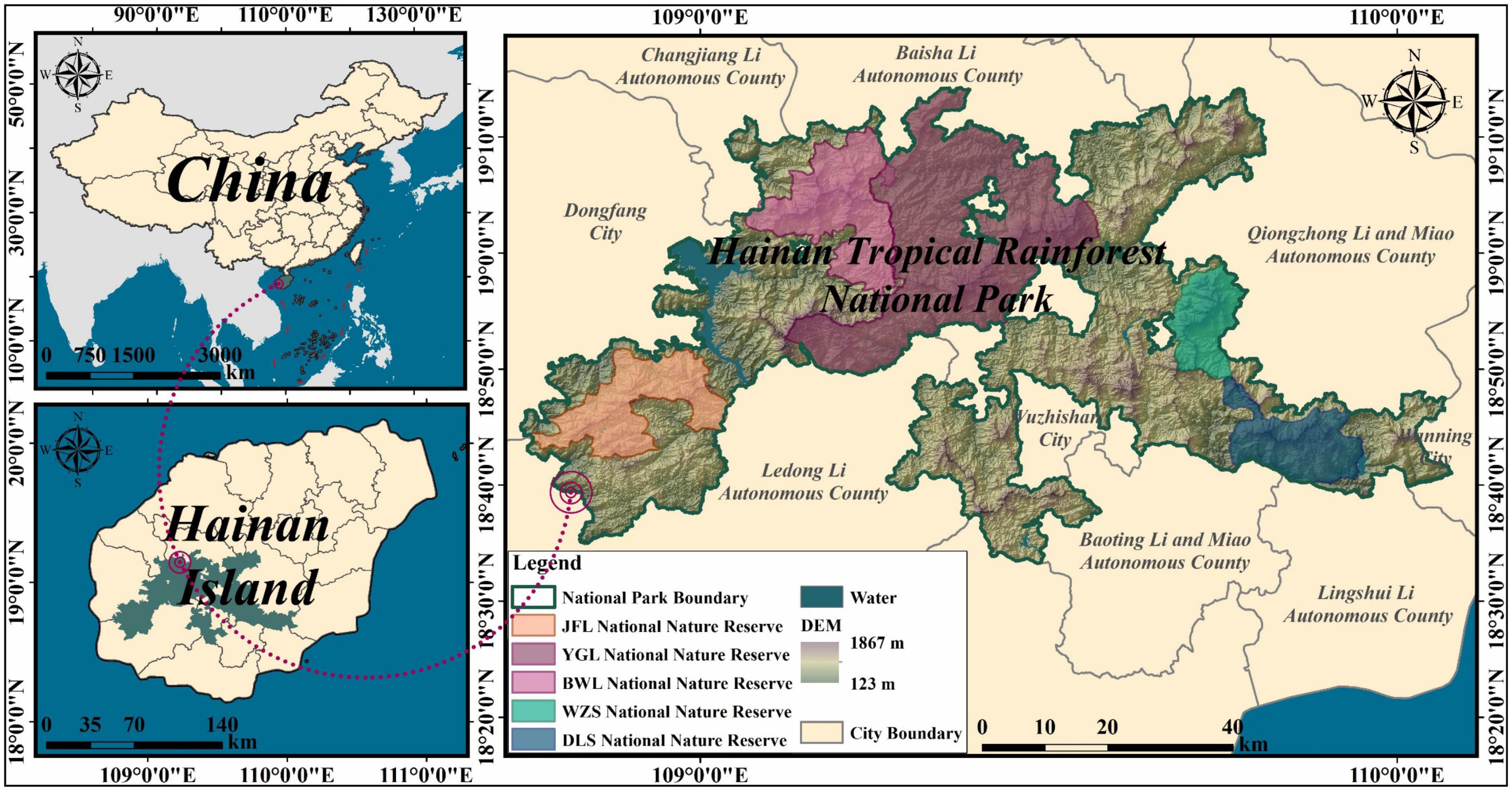
Figure 1. Location of the study area. JFL, Jianfengling; YGL, Yinggeling; BWL, Bawangling; WZS, Wuzhishan; DLS, Diaoluoshan.

The unique geographical and climatic environment has shaped China’s precious tropical rainforest ecosystem. Since the establishment of Hainan as a province in 1988, the implementation of a series of strategies, such as the construction of Hainan International Tourism Island, has promoted the economic development of cities and counties, which is bound to bring a certain degree of impacts on the landscape patterns of the HTRNP, and then affect some essential ESs related to human well-being. Therefore, it is urgent to quantitatively assess the landscape pattern changes in the HTRNP and its impacts on the critical ESs benefits.

2.2. Data sources and processing

Multi-source datasets were adopted in this study (Table 1). The land use/land cover (LULC) data comes from China’s Multi-Period Land Use/Land Cover Remote Sensing Monitoring Dataset (CNLUCC) (Xu et al., 2018), and the spatial resolution is 30 m. We unified all the raster data to a spatial resolution of 30 m based on the ArcGIS v10.2 platform, and the projection coordinate system was unified to WGS_1984_Albers. The framework of this study is shown in Figure 2.

TABLE 1

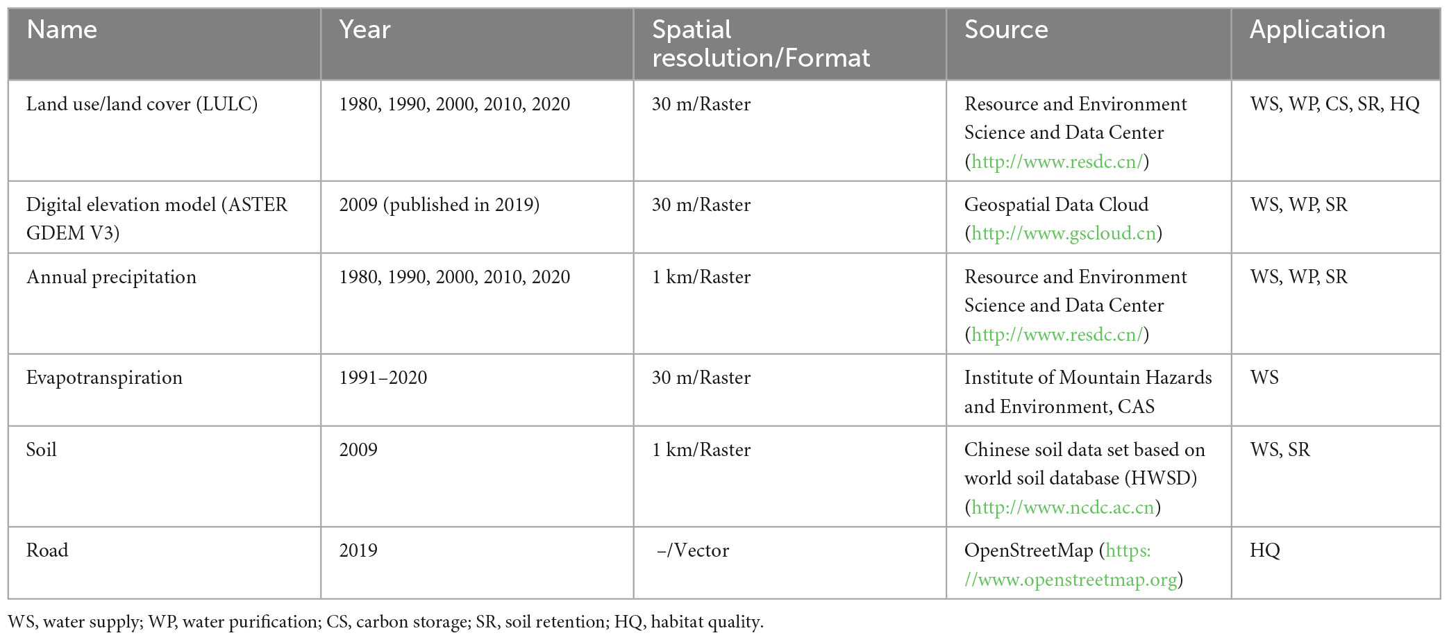
Table 1. Data information.

FIGURE 2

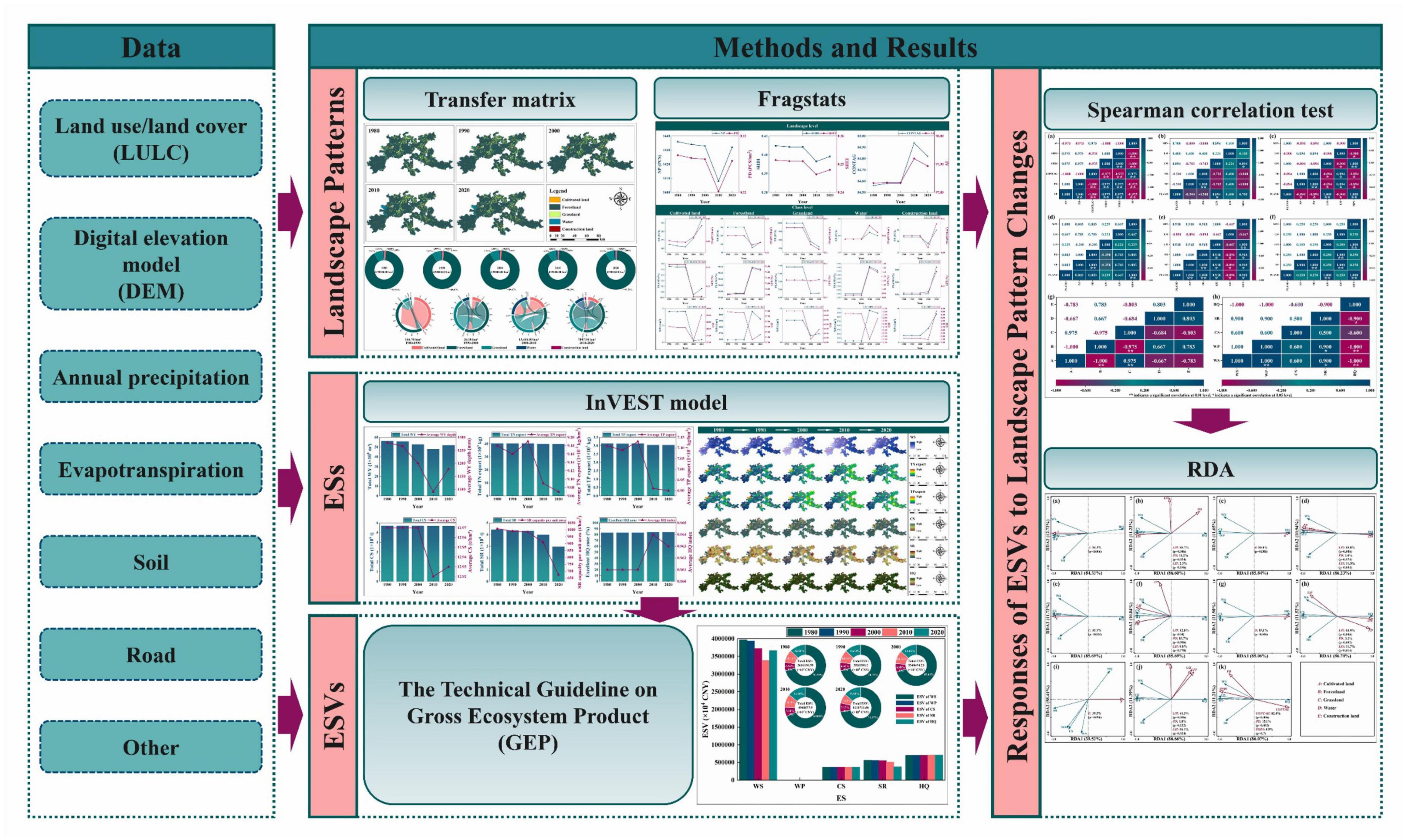
Figure 2. The framework of this study.

2.3. Landscape patterns analysis

2.3.1. Analysis of landscape type changes

Based on the LULC data, the landscape types of HTRNP were divided into five categories: cultivated land, forestland, grassland, water, and construction land. This study used the transfer matrix to analyze the landscape types transition in two adjacent time nodes (1980–1990, 1990–2000, 2000–2010, and 2010–2020) during 1980–2020.

2.3.2. Analysis of landscape index changes

Based on the actual situation of HTRNP and related study (Li L. et al., 2022), ten landscape indices were selected from Landscape and Class levels: percent of landscape (PLAND), number of patches (NP), patch density (PD), mean patch size (MPS), landscape shape index (LSI), largest patch index (LPI), Shannon’s diversity index (SHDI), Shannon’s evenness index (SHEI), contagion (CONTAG), and aggregation index (AI). These indices were calculated based on Fragstats v4.2 platform.

2.4. ES indicators selection and assessment

With reference to the ES classification system of The Economic of Ecosystems and Biodiversity (TEEB), and considering the availability and accessibility of data, this study finally selected five important ES indicators based on the characteristics of HTRNP: (1) water supply (WS) and water purification (WP): HTRNP is the source of three major rivers (Nandu, Changhua, and Wanquan) and the primary water source of two major reservoirs (Songtao and Daguangba) on Hainan Island, the WS and WP services of HTRNP is essential for maintaining and regulating the hydrological services of island-wide ecosystems (Li A. et al., 2022); (2) carbon storage (CS), soil retention (SR), and habitat quality (HQ): HTRNP has preserved the largest tropical rainforest and monsoon rainforest ecosystem in China, it is not only the most significant carbon pool of Hainan Island, but also plays a vital role in soil conservation and biodiversity protection (Yu et al., 2016); the abundant rainfall in HTRNP increases the potential risk of soil erosion and poses a threat to biological habitats. The Integrated Valuation of Ecosystem Services and Tradeoffs (InVEST) (Tallis and Polasky, 2009; Sharp et al., 2016) model has been widely used for the ESs assessment, so we applied InVEST v3.12 model to evaluate the biophysical values of the above five ESs. And referring to “The Technical Guideline on Gross Ecosystem Product (GEP)” issued by the Ministry of Ecology and Environment of the People’s Republic of China in 2020, and related research (Chen et al., 2021), the assessment methods (including biophysical and monetary values) of the five ES indicators for HTRNP were established (Table 2).

TABLE 2

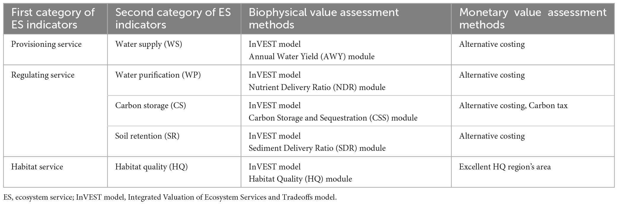
Table 2. Ecosystem service indicators and assessment methods for HTRNP.

2.4.1. Water supply

The biophysical value of WS was assessed using the AWY module. This module is based on the water balance principle and considers several factors, such as transpiration, evaporation, and precipitation. The calculation formula is as follows:

$Y_{xj}=(1-\frac{AE{T}_{xj}}{P_x})\times P_x$

where Y_xj is the annual water yield on the pixel x of the landscape type j (mm); AET_xj is the actual annual evapotranspiration on the pixel x of the landscape type j (mm); P_x is the annual precipitation on the pixel x (mm) (Qi et al., 2019). The maximum root depth (Root_depth), plant evapotranspiration coefficient (K_c), and actual evapotranspiration value (LULC_veg) in the biophysical coefficient table (Supplementary Table 1) were set according to Zheng et al.’s (2019) research on the central mountainous region of Hainan Island. Zhang’s coefficients for each year were set by referring to the measured data of the Fucai hydrological station in HTRNP (Li A. et al., 2022) after several adjustments. The monetary value of WS was assessed using Alternative costing method. The calculation formula is as follows:

$V_{ws}=Q_{ws}\times C$

where V_ws is the monetary value of WS (CNY/a); Q_ws is the total annual water supply (m³/a); C is the engineering cost of reservoir constructing per unit capacity (CNY/m³). According to the “Yearbook of China water resources,” the average reservoir capacity cost is 2.17 CNY/m³, then C was calculated as 7.0547 CNY/m³ based on the 2009 price index (3.251) (Fang et al., 2013).

2.4.2. Water purification

The biophysical value of WP was assessed using the NDR module, which inversely characterizes the WP service function by the total nitrogen (TN) and total phosphorus (TP) exports. The higher the TN and TP exports per unit area, the weaker the WP service function. The calculation formula is as follows:

$AL{V}_x=HS{S}_x\times po{l}_x$

$HS{S}_x={\mathrm{\lambda }}_x/\overline{{\mathrm{\lambda }}_w}$

where ALV_x is the adjusted loading value on the pixel x; pol_x is the export coefficient on the pixel x; HSS_x is the hydrologic sensitivity score on the pixel x, λ_x is the runoff index on the pixel x, $\overline{{\mathrm{\lambda }}_w}$ is the average runoff index in the watershed of interest (Qi et al., 2019). Nitrogen (N) and phosphorus (P) export coefficients and retention efficiency (Supplementary Table 2) for landscape types were set with reference to relevant studies (Zhe et al., 2013; Zheng et al., 2019). The monetary value of WP was assessed using Alternative costing method. The calculation formula is as follows:

$V_{wp}=\sum T_N\times P_N+\sum T_P\times P_P$

where V_wp is the monetary value of WP (CNY/a); T_N and T_P are the total amount of TN and TP purification (t/a); P_N and P_P are the purification unit-prices of TN and TP (CNY/t), and the values are 1,750 and 2,800 CNY/t, respectively, according to the “Levy standard of pollution discharge fees and calculation methods” of the National Development and Reform Commission of China (Fan and Li, 2020).

2.4.3. Carbon storage

The biophysical value of CS was assessed using the CSS module, which estimates CS based on each landscape type and its corresponding four primary carbon pools. The calculation formula is as follows:

$C_{total}=C_{above}+C_{below}+C_{soil}+C_{dead}$

where C_total is the total CS (t/hm²); C_above, C_below, C_soil, and C_dead are aboveground CS (t/hm²), belowground CS (t/hm²), soil CS (t/hm²), and dead organic CS (t/hm²), respectively. As the vegetation of HTRNP is mainly evergreen broad-leaved species of zonal forest type, its dead organic CS is tiny and difficult to estimate (Gong et al., 2022). This part of CS was not calculated in this study. Other three types of carbon density were set (Supplementary Table 3) with reference to Liu et al.’s (2022) study. The monetary value of CS was assessed using a combination of Alternative costing and Carbon tax methods. The calculation formula is as follows:

$V_{cs}=(272.65C_t+1017.675C_t)/2$

where V_cs is the monetary value of CS (CNY/a); C_t is the total CS (t/a). To obtain more accurate monetary value assessment results, this study referred to Wang et al.’s (2017) study, the unit-price of forest carbon sink in Alternative costing method used the arithmetic average of four unit-prices (251.40, 260.90, 273.30, and 305.00 CNY/t); the Carbon tax method used the international Swedish carbon tax rate (150 USD/t = 1,017.675 CNY/t, the exchange rate was calculated as 100 USD = 678.45 CNY on 29 January 2023).

2.4.4. Soil retention

The SDR module assesses SR’s biophysical value based on the Revised Universal Soil Loss Equation (RUSLE). The calculation formula is as follows:

$A_x=R_x\times K_x\times L{S}_x\times (1-C_x\times P_x)$

$R_j=0.0534P_j^{1.6548}$

$K=(-0.01383+0.51575K_{EPIC})\times 0.1317$

where A_x is the SR amount on the pixel x (t⋅hm^–2⋅a^–1); R_x is the rainfall erosivity factor on the pixel x (MJ⋅mm⋅hm^–2⋅h^–1⋅a^–1); K_x is the soil erodibility factor on the pixel x (t⋅hm²⋅h⋅hm^–2⋅MJ^–1⋅mm^–1); LS_x is the topographical factor on the pixel x; C_x is the crop-management factor on the pixel x; P_x is the support practice factor (Qi et al., 2019). R was calculated using the rainfall erosion force model (Zhang and Fu, 2003), R_j is the rainfall erosion force in year j (MJ⋅mm⋅hm^–2⋅h^–1⋅a^–1), P_j is the rainfall in year j (mm). K was calculated using the Erosion-Productivity Impact Calculator (EPIC) model (Williams, 1995), the K_EPIC was corrected according to Zhang et al. (2008). The values of C and P were set (Supplementary Table 4) according to the relevant studies (Xiao, 1999; Zheng et al., 2019). The monetary value of SR (including the value of both sedimentation reduction and non-point source pollution reduction) assessed using the Alternative costing method. The calculation formula is as follows:

$V_{sr}=V_{sd}+V_{dpd}$

$V_{sd}=\mathrm{\lambda }\times (Q_{sr}/\mathrm{\rho })\times C$

$V_{dpd}=\sum _{i=1}^2{Q}_{sr}\times C_i\times P_i$

where V_sr is the monetary value of SR (CNY/a); V_sd is the value of sedimentation reduction (CNY/a); V_dpd is the value of non-point source pollution reduction (CNY/a); λ is the sedimentation coefficient, taking the value of 0.24 (Sheng et al., 2010); Q_sr is the SR amount (t/a); C is the cost of reservoir desilting project per unit area (CNY/m³), according to the “The building built water engineering budget norm” of the Ministry of Water Resources of the People’s Republic of China, the value of C is 17.63 CNY/m³ (Yu et al., 2020); ρ is the soil capacity (t/m³), according to the average of the measured data of each forest ecosystem type in the central mountainous region of Hainan island in 2008, the value of ρ is 1.28 t/m³ (Liu et al., 2009); C_i is the pure content of N (or P) in soil (%), and it was determined that the content of N and P in soil of China are 0.370 and 0.108%, respectively (Wang L. et al., 2017); P_i is the degradation cost of N (or P), according to the “Levy standard of pollution discharge fees and calculation methods,” the degradation costs of N and P are 1,750 and 2,800 CNY/t, respectively (Fan and Li, 2020).

2.4.5. Habitat quality

The biophysical value of HQ was assessed using the HQ module. The value of the HQ index is in the range of [0,1], and the higher value indicates the higher level of biodiversity. The calculation formula is as follows:

$Q_{xj}=H_j(1-\frac{D_{xj}^z}{D_{xj}^z+K^z})$

where Q_xj is the HQ on the pixel x of the landscape type j; H_j is the habitat suitability of the landscape type j; D_xj is the total threat level on the pixel x of the landscape type j; K is the half-saturation coefficient, generally taking a value of 0.5; z is a scaling factor, generally taking a value of 2.5 (Yang et al., 2021). Referring to the studies on HTRNP and its neighboring regions (Lei et al., 2022; Yao et al., 2022), paddy fields, dry land, rural residential areas, other construction lands, and expressways were selected as threat factors in this study. The impact distance and weight of the threat factors (Supplementary Table 5) and the sensitivity of each landscape type (Supplementary Table 6) were set with reference to the model manual and the above studies. Referring to related research (Xiao et al., 2014; Sun et al., 2019), the monetary value of HQ was assessed based on the area of excellent HQ regions, and the ecological benefit of the excellent HQ region is about 191.28 × 10⁴ CNY/km². The excellent HQ regions were obtained by referring to Lei et al.’s (2022) study using the Natural Breaks method to classify the HQ spatial distribution into four classes (Poor: 0–0.3, Medium: 0.3–0.7, Good: 0.7–0.9, and Excellent: 0.9–1.0).

2.5. Correlation mechanism analysis between ESVs and landscape patterns

2.5.1. Correlation test between variables

Testing whether there is a correlation between landscape indices and various types of ESVs is a critical a priori step in exploring the correlation between ESVs and landscape pattern changes, to test whether correlations exist among variables, whether the direction and magnitude of the correlations are as expected, and whether they apply to subsequent more complex multivariate analyses (Cen, 2016; Ge, 2020).

2.5.2. Ranking analysis of the correlation between ESVs and landscape patterns

The ranking analysis is widely used in ecological studies to explain the response relationships between species and environmental variables, this method can effectively downscale the multi-dimensional information, and its analysis results are concise and intuitive (Legendre, 2008; Cen, 2016). According to the results of DCA (length of gradient <3), this study applied the Redundancy Analysis (RDA) based on the Canoco v5.0 platform to rank the correlation between ESVs and landscape patterns. The RDA is a ranking analysis method combining regression and Principal Component Analysis (PCA). It is an extension of multiple regression analysis and can be used to model multivariate response data. The RDA ranking chart can visualize the relationship between environment and response variables (Rao et al., 2016). The angle between their arrows reflects the correlation between them: when the angle <90°, it indicates a positive correlation between the variables, and the smaller the angle, the stronger the positive correlation; when the angle >90°, it indicates a negative correlation between the variables, and the larger the angle, the stronger the negative correlation; when the angle = 90°, it shows that the variables are not correlated with each other (Li C. et al., 2022).

3. Results

3.1. Landscape pattern changes

3.1.1. Landscape type changes from 1980 to 2020

From both the distribution (Figure 3) and proportion (Figure 4) of landscape types, forestland is the most dominant landscape type in the HTRNP, followed by grassland, and construction land occupies a minor proportion. During 1980–2020, the proportion of forestland fluctuated between 89.86 and 90.29%, with little overall change; the proportion of cultivated land, grassland, and water changed relatively significantly. The conversion between different landscape types became frequent after 2000, especially during 2000–2010. The total area conversion reached 13,446.00 hm² and then gradually eased after 2010.

FIGURE 3

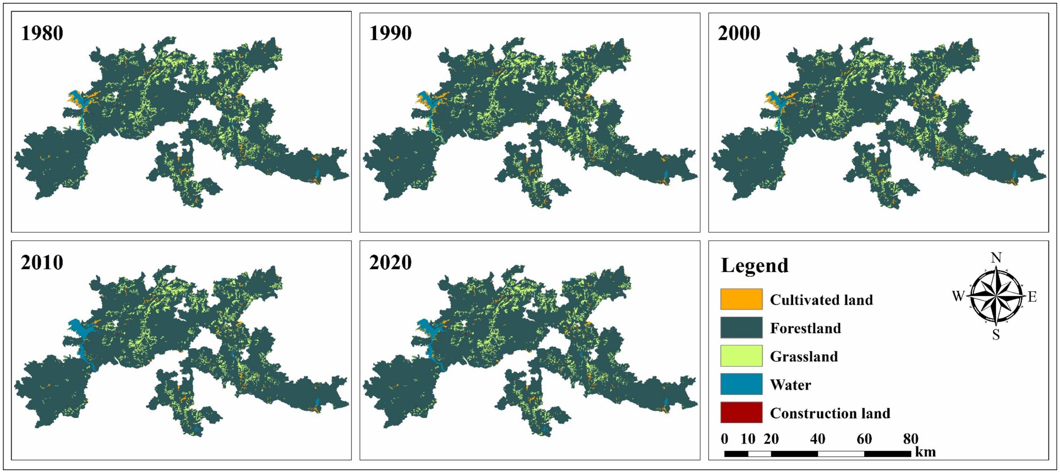
Figure 3. Spatial distribution of landscape types in HTRNP during 1980–2020.

FIGURE 4

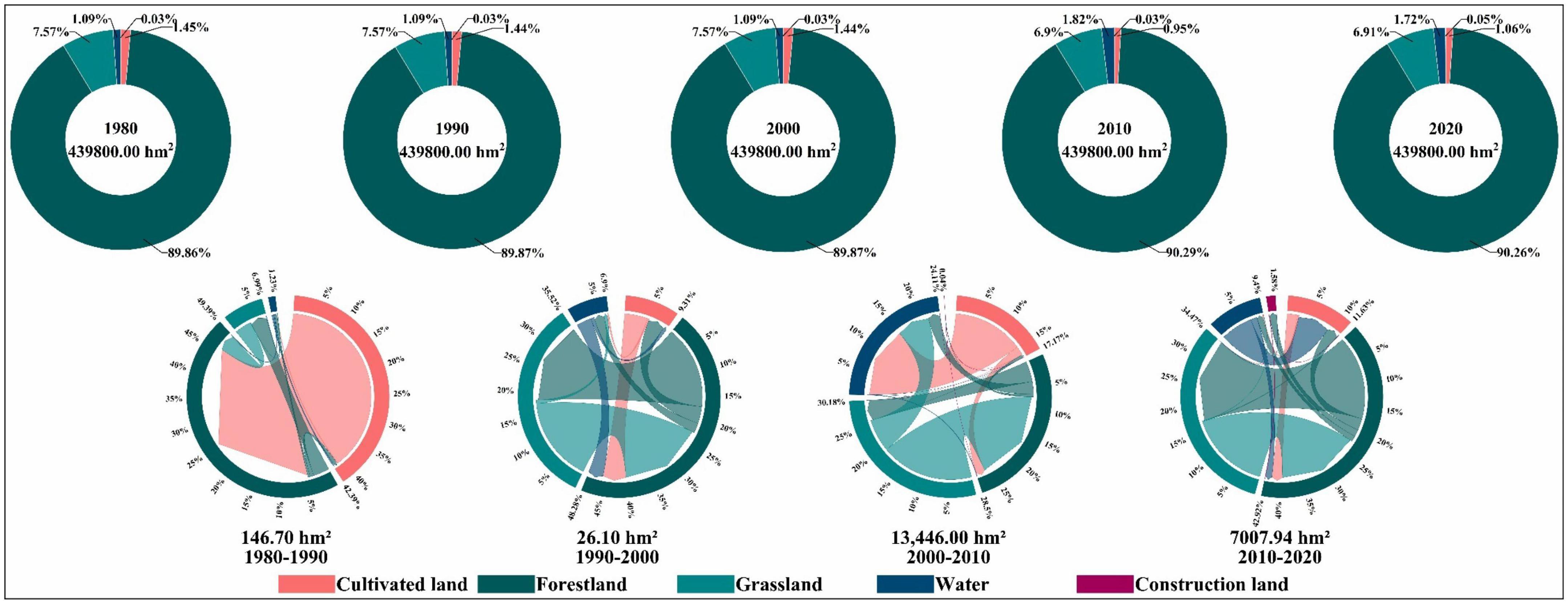
Figure 4. Landscape type changes in HTRNP during 1980–2020.

(1) During 2000–2010, grassland, cultivated land, and forestland areas were transferred out more obviously, accounting for 52.06, 33.18, and 14.72% of the total area transferred out, respectively. Although forestland was one of the primary sources of transfer out area, its proportion showed positive growth because of the significant area input of grassland and cultivated land (Figure 4). The conversions of cultivated land in the northwest and grassland in the southeast to water and forestland, respectively, were evident (Figure 3). (2) The magnitude of changes in landscape types during 2010–2020 was less than in the previous period (Figure 4), and spatially (Figure 3), only the conversion of part of the northwestern water to cultivated land was slightly noticeable. Although the conversion between forestland and grassland was apparent (Figure 4), the main areas’ conversion was limited between these two types, and the number of areas transferred between them was similar. Hence, the changes in the proportion of these two types were relatively small.

3.1.2. Landscape index changes from 1980 to 2020

During 1980–2020, at the Landscape level (Figure 5): NP and PD showed a trend of “slow decline – rapid decline – rapid rise,” with a slight overall decline, indicating that landscape fragmentation and heterogeneity of HTRNP tended to decline; SHDI and SHEI showed a trend of “slow decline – rapid decline – slow rise,” with an overall decline, indicating that the homogeneity of the HTRNP’s landscape decreased, the dominant landscape patch types tended to be prominent, and the distribution of landscape patch types in HTRNP tended to be uneven, which may be related to the shrinkage of both grassland and cultivated land and the expansion of both forestland and water. CONTAG and AI showed a trend of “slow rise – rapid rise – slow decline,” these two indices tended to increase overall, indicating that the connectivity of the dominant landscape in HTRNP was enhanced, and the degree of landscape agglomeration was increased.

FIGURE 5

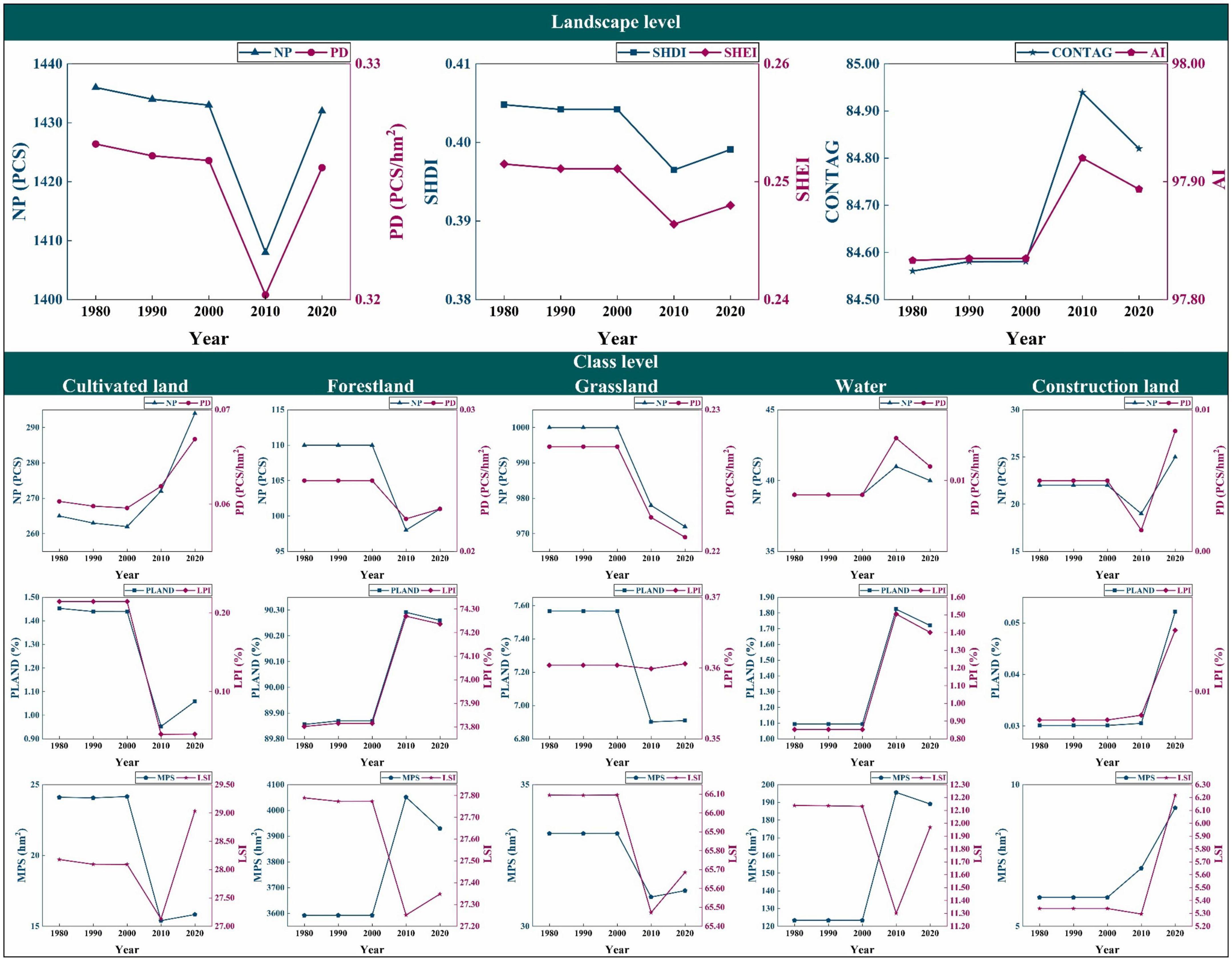
Figure 5. Landscape index changes in HTRNP during 1980–2020. PLAND, percent of landscape; NP, number of patches; PD, patch density; MPS, mean patch size; LSI, landscape shape index; LPI, largest patch index; SHDI, Shannon’s diversity index; SHEI, Shannon’s evenness index; CONTAG, contagion; AI, aggregation index.

At the Class level (Figure 5): (1) Cultivated land: NP and PD tended to increase, PLAND, LPI, and MPS tended to decrease, indicating that the cultivated land tended to be fragmented and its landscape dominance decreased; LSI tended to increase, indicating that the landscape shape tended to be complex. (2) Forestland: NP and PD tended to decrease, indicating an increase in forestland aggregation; the three indices of PLAND, LPI, and MPS of forestland were the highest among the five landscape types, and all tended to increase, indicating the landscape pattern of HTRNP were dominated by large patches of forestland, and the landscape dominance of forestland tended to increase; LSI tended to decrease, indicating its landscape shape become more regularized. (3) Grassland: grassland had the highest NP and PD among the five landscape types, indicating the highest degree of fragmentation in grassland landscape, but its fragmentation tended to decrease; LPI changed less, PLAND and MPS tended to decrease, indicating a decrease in its fragmentation was related to the conversion of some small scattered patches to other landscape patch types; LSI tended to decrease, indicating that the landscape shape tended to be regularized. (4) Water: NP and PD tended to increase but at a lower rate; PLAND, LPI, and MPS all tended to increase, indicating an increase in landscape dominance; LSI tended to decrease in general, indicating that the landscape shape tended to be regularized. (5) Construction land: NP, PD, PLAND, LPI, and MPS increased slightly, indicating its area was increasing in fragmented patches; LSI tended to increase, indicating its shape became complex. In summary, landscape indices at both levels changed significantly during 2000–2020.

3.2. Spatial-temporal changes of ESs

3.2.1. Temporal changes of ESs from 1980 to 2020

All the five ESs of HTRNP showed varying degrees of trends during 1980–2020 (Figure 6).

FIGURE 6

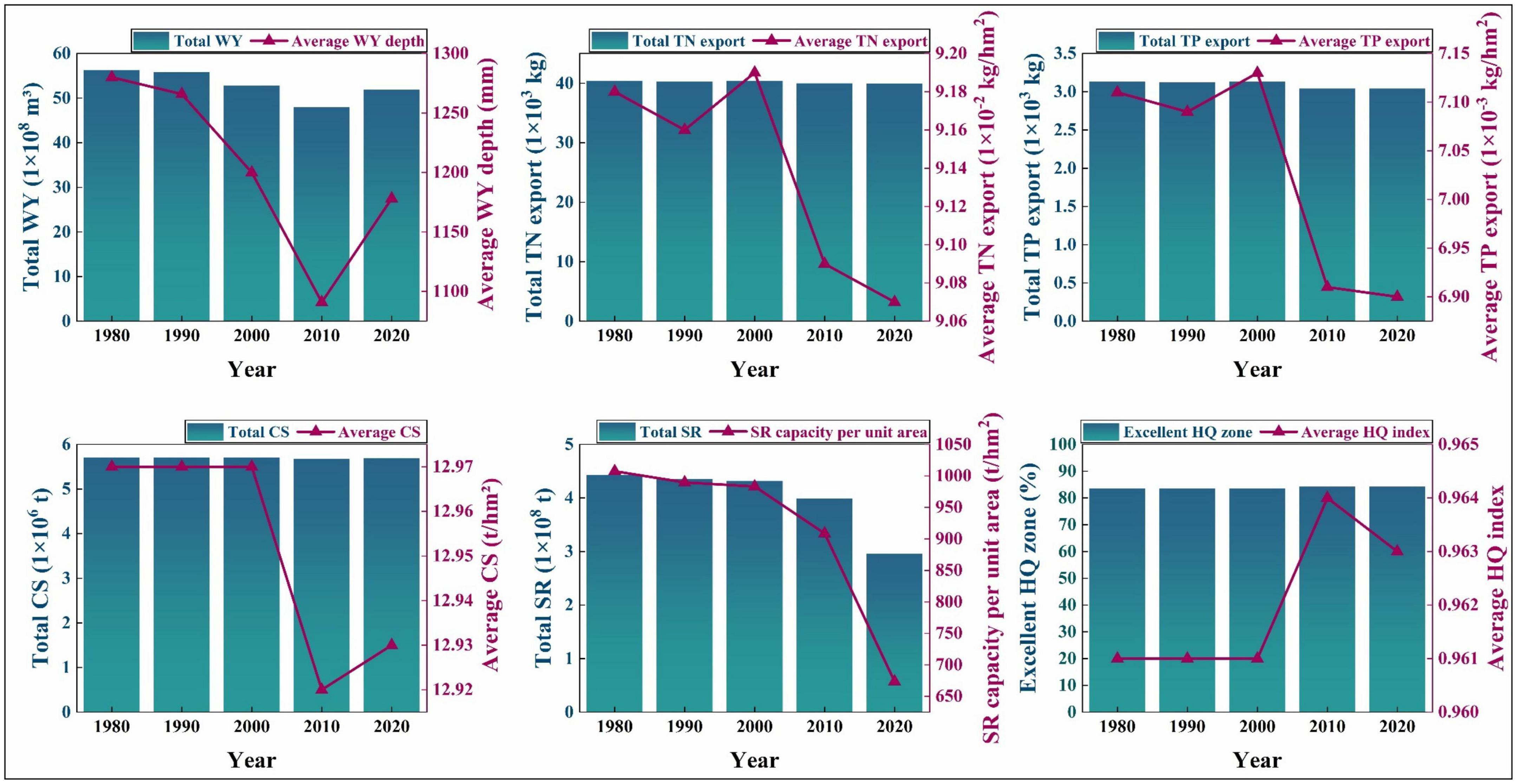
Figure 6. Temporal changes of ESs in HTRNP during 1980–2020. WY, water yield; TN, total nitrogen; TP, total phosphorus; CS, carbon storage; SR, soil retention; HQ, habitat quality.

(1) WS: WS’s biophysical value decreased continuously during 1980–2010; the decrease was more evident during 1990–2010, the total WY decreased by 14.16%, and the average WY depth decreased from 1,265.83 to 1,090.93 mm; it rebounded after 2010. There has been a declining trend in WS over the past 40 years, with total annual WY decreasing by 7.82%. (2) WP: the average TN and TP exports both decreased rapidly during 2000–2010, with the average TN export decreasing from 9.19 × 10^–2 kg/hm² to 9.09 × 10^–2 kg/hm² and the average TP export decreasing from 7.13 × 10^–3 kg/hm² to 6.91 × 10^–3 kg/hm². The total exports of both TN and TP had decreased slightly over the past 40 years, by 1.24 and 2.88%, respectively. (3) CS: the average CS declined rapidly during 2000–2010, from 12.97 t/hm² to 12.92 t/hm², and the total CS decreased by 0.53%; it rebounded slightly after 2010. There has been a slight overall downward trend in CS over the past 40 years, with a total reduction of 0.35%. (4) SR: the biophysical value of SR decreased significantly during 2010–2020, with a 25.81% decrease in total SR and a decrease in SR capacity per unit area from 908.68 t/hm² to 673.60 t/hm². SR decreased from 1980 to 2020, and the total SR decreased by 33.18%. (5) HQ: the biophysical value of HQ rose rapidly during 2000–2010, with the average HQ index peaking at 0.964; it dropped slightly to 0.963 after 2010. The overall HQ remained high and tended to increase during 1980–2020, the proportion of excellent HQ zone remained above 80%, and the average HQ index remained above 0.960.

3.2.2. Spatial changes of ESs from 1980 to 2020

The mean values of ESs at the sub-watershed scale were calculated based on the Zonal Statistics tool of ArcGIS v10.2 platform, and the ESs were normalized from 0 to 1 (Low to High) for each year to facilitate comparison across years (Xia et al., 2023). All five ESs of HTRNP showed different degrees of spatial heterogeneity during 1980–2020 (Figure 7).

FIGURE 7

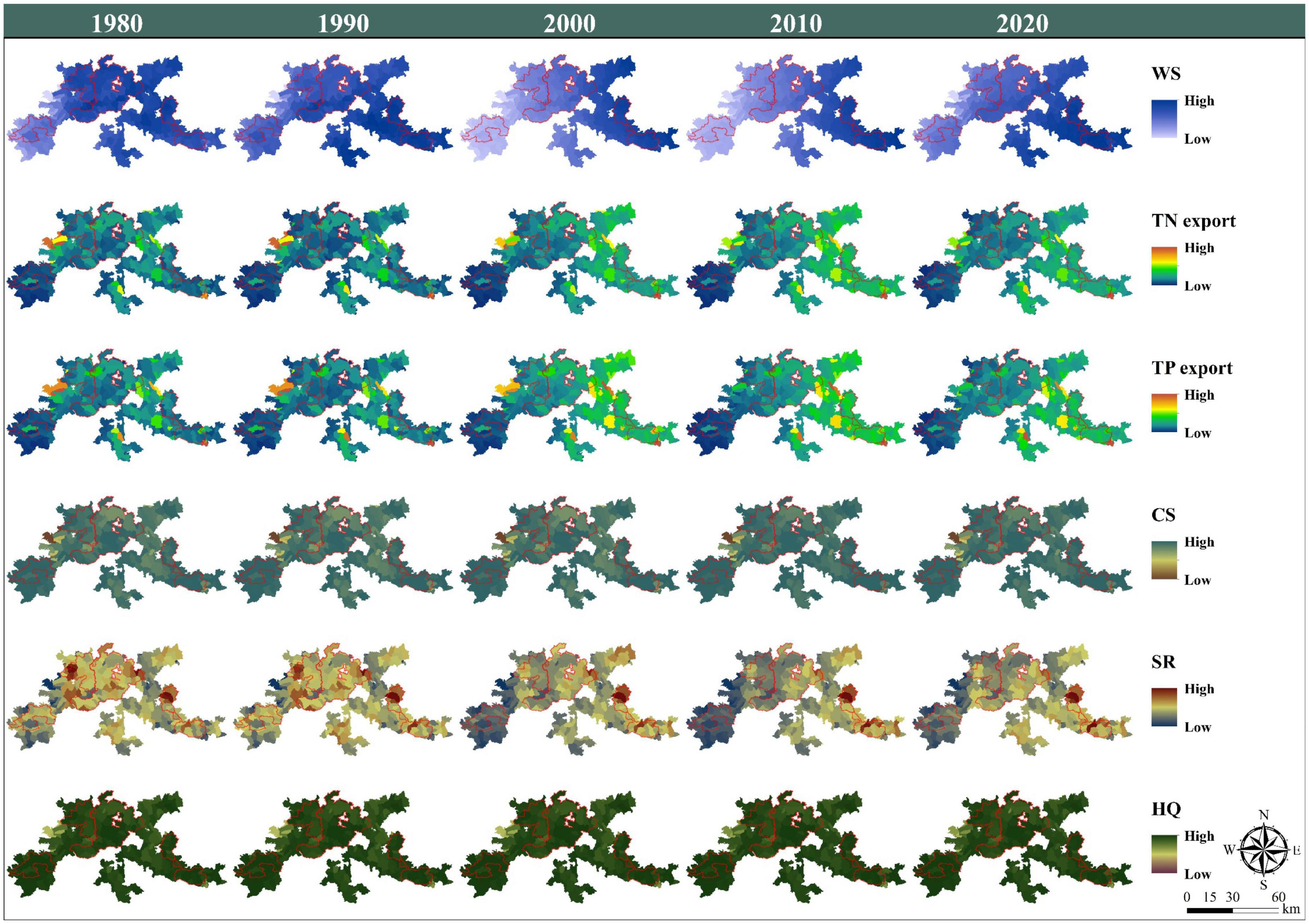
Figure 7. Spatial patterns of ESs in HTRNP during 1980–2020. WS, water supply; TN, total nitrogen; TP, total phosphorus; CS, carbon storage; SR, soil retention; HQ, habitat quality.

(1) WS: the spatial heterogeneity of WS is “high in the east and low in the west.” This spatial heterogeneity tended to be significant during 2000–2010, the WS in the southwestern region (including JFL NNR) continued to decrease, and the low-value regions expanded toward the BWL and YGL NNRs in the central region. This trend decreased in 2020. The high-value regions were mainly concentrated in the southeast (including WZS and DLS NNRs). (2) WP: the spatial distribution of both TN and TP exports showed a gradient pattern increasing from the southwestern region (including JFL NNR) to the central region (including BWL and YGL NNRs) and then to the southeastern region (including WZS and DLS NNRs). The high-value regions in the northwest showed a transformation trend to the low-value regions. (3) CS: CS’s spatial heterogeneity did not vary significantly, the low-value regions were concentrated in the northwest, and the high-value regions were concentrated in the southwest (including JFL NNR). (4) SR: SR’s spatial heterogeneity was observed. The low-value regions in the southwest (including JFL NNR) showed a significant expansion during 2000–2010. This trend decreased in 2020. (5) HQ: the spatial heterogeneity of HQ was not observed and did not change significantly. Relatively, the HQ in the northwestern region was slightly lower.

3.3. ESV changes from 1980 to 2020

The total ESV has decreased over the past 40 years (Figure 8), with the most significant decrease during 2000–2010 and a slight rebound in 2020, with a total reduction of 494,419.03 × 10⁴ CNY. The trends of ESVs are the same as those of ESs: (1) WS’s ESV tended to decrease, but its value weight was still the highest among all ESVs, which may be related to the particular topography and climate of HTRNP: the high altitude and rugged terrain of the HTRNP have a lifting effect on moist air currents, resulting in significant rainfall, and the high altitude also results in low evapotranspiration, all of which contribute to higher WS (Xia et al., 2023). (2) WP’s ESV showed a slight decrease, its value weight was almost 0%, and this may be related to the low TN and TP loads in HTRNP: most of the regions in the HTRNP are sloping and unsuitable for cultivation, so the area of cultivated land is relatively small, resulting in less nitrogen and phosphorus loading from agricultural surface runoff, and thus the amount of purification is less, leading to a low ESV of WP Zhe et al. (2013). (3) CS’s ESV declined slightly. Its value weight fluctuated around 7% with insignificant changes. (4) SR’s ESV continued to decrease, with a significant drop during 2010–2020, and its value weight plummeted to about 7%, close to that of CS. (5) HQ’s ESV tended to increase slightly, and its value weight tended to rise, second only to WS. This phenomenon demonstrated the overall better HQ of HTRNP and indicated that the HQ service was gradually being valued.

FIGURE 8

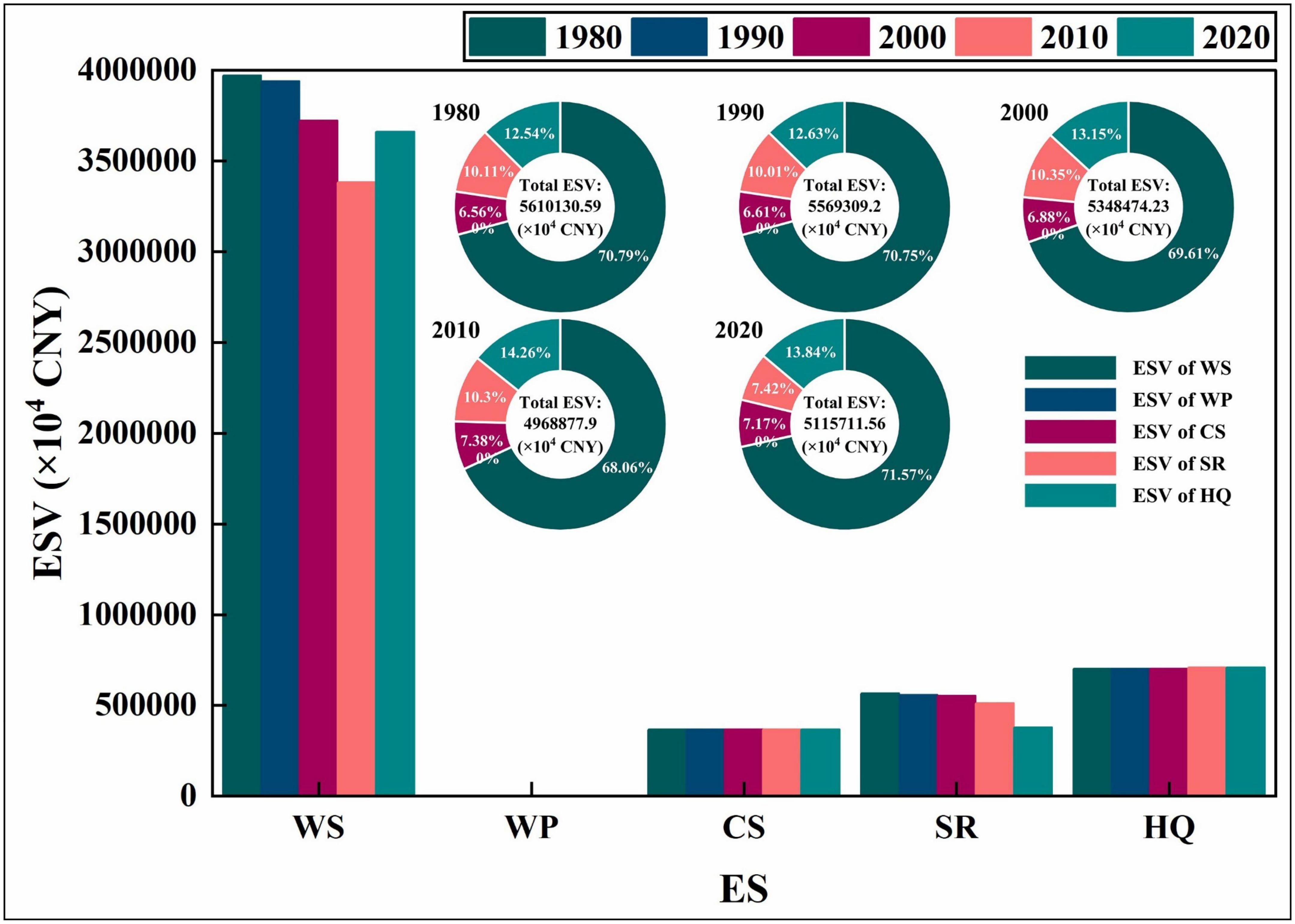
Figure 8. Ecosystem service value changes in HTRNP during 1980–2020. ES, ecosystem service; ESV, ecosystem service value; WS, water supply; WP, water purification; CS, carbon storage; SR, soil retention; HQ, habitat quality.

3.4. Analysis of the correlation mechanism between ESVs and landscape patterns

3.4.1. Correlation test between variables

The landscape indices, landscape areas, and ESVs of HTRNP during 1980–2020 were used as data sources to test the correlation between these variables. The correlation test was performed based on the IBM SPSS Statistics v26 platform, using the Spearman correlation coefficient as a measure and a two-tailed t-test for the significance of the correlation coefficient. The results showed (Supplementary Figure 1) that the variables had different degrees of correlation.

Based on the previous analysis of the HTRNP’s landscape pattern changes, it can be noted that the trends between some of the indices are very similar, indicating that there may be some degree of correlation between them. The strong correlation between indices will result in indices that do not satisfy the statistical properties of mutual independence, causing duplication and redundancy in the mathematical and theoretical significance of subsequent studies, thus affecting the accuracy of the results (Cen, 2016; Ge, 2020). Therefore, in this study, the landscape indices with low correlations were further screened based on the results of the correlation test for subsequent ranking analysis: (1) Landscape level: PD, SHDI, and CONTAG; (2) Class level: PD, LPI, and LSI.

3.4.2. Ranking analysis of the correlation between ESVs and landscape patterns

The RDA ranking analysis (Figure 9) was conducted based on the Canoco v5.0 platform using ESVs as response variables and the landscape areas and indices as environmental variables. Based on the correlation test results between landscape indices, the environmental variable groups are as follows: (1) Landscape level: PD, SHDI, and CONTAG; (2) Class level: LPI, PD, and LSI.

FIGURE 9

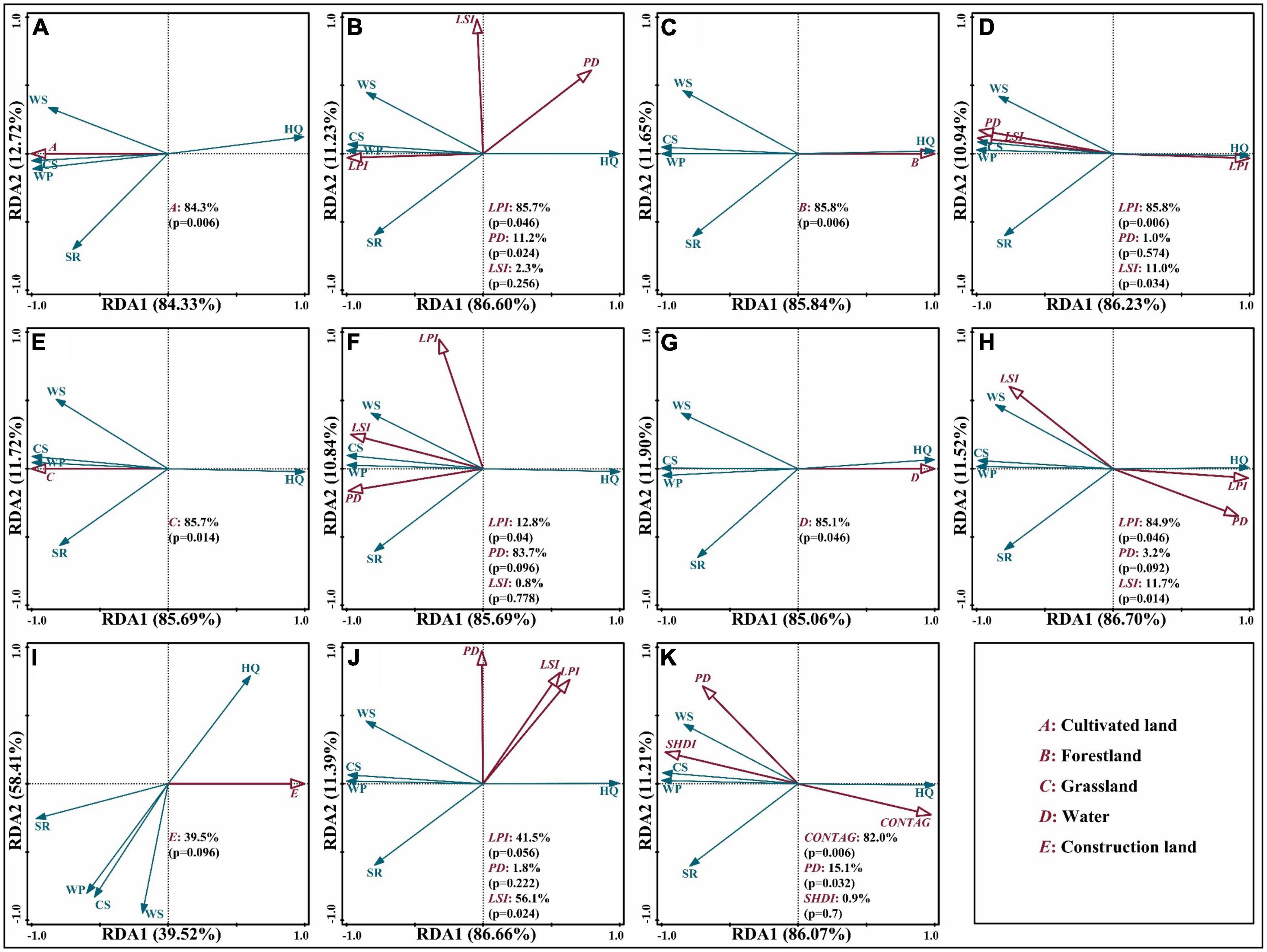
Figure 9. Redundancy analysis ranking chart. (A) cultivated land area; (B) landscape indices of cultivated land; (C) forestland area; (D) landscape indices of forestland; (E) grassland area; (F) landscape indices of grassland; (G) water area; (H) landscape indices of water; (I) construction land area; (J) landscape indices of construction land; (K) landscape indices at landscape level. WS, water supply; WP, water purification; CS, carbon storage; SR, soil retention; HQ, habitat quality; PD, patch density; SHDI, Shannon’s diversity index; CONTAG, contagion; LPI, largest patch index; LSI, landscape shape index.

(1) The changes of landscape types over the past 40 years have impacted ESVs. The explanatory degree of cultivated land (84.3%), forestland (85.8%), grassland (85.7%), and water (85.1%) areas are all higher to ESVs, indicating that changes in these four landscape types had significant effects on ESVs. In comparison, the explanatory degree of construction land (39.5%) area is lower, indicating that its changes had weaker effects on ESVs, which may be related to its small area. WP and CS have a strong positive correlation with the areas of grassland and cultivated land and a strong negative correlation with the areas of forestland and water; SR has a strong negative correlation with the area of construction land; HQ has a strong positive correlation with the areas of forestland and water and a strong negative correlation with the areas of grassland and cultivated land.

(2) At the Class level: landscape indices’ effects on ESVs across landscape types vary.

Cultivated land: the explanation degree of LPI to ESVs is the highest, reaching 85.7%, followed by PD; LSI has the lowest explanatory degree and did not explain changes in ESVs significantly (p > 0.10), and also had a weak correlation with ESVs. WP-LPI and CS-LPI have strong positive correlations, while HQ-LPI and SR-PD have strong negative correlations.

Forestland: the explanation degree of LPI to ESVs is the highest, reaching 85.8%, followed by LSI; PD has the lowest explanatory degree and did not explain changes in ESVs significantly (p > 0.10). WP-LSI, CS-LSI, and HQ-LPI have strong positive correlations, while WP-LPI, CS-LPI, and HQ-LSI have strong negative correlations.

Grassland: the explanation degree of PD to ESVs is the highest, reaching 83.7%, followed by LPI; LSI has the lowest explanatory degree and did not explain changes in ESVs significantly (p > 0.10). WP-PD and CS-PD have strong positive correlations, while HQ-PD has strong negative correlations.

Water: the explanation degree of LPI to ESVs is the highest, reaching 84.9%, followed by LSI; PD has the lowest explanatory degree. HQ-LPI has strong positive correlations, while WP-LPI and CS-LPI have strong negative correlations.

Construction land: compared with other landscape types, the explanatory degrees of landscape indices of construction land to ESVs are lower. The index with the highest explanatory degree is LSI (explanatory degree only reached 56.1%), followed by LPI; PD has the lowest explanatory degree and did not explain changes in ESVs significantly (p > 0.10). SR-LSI and SR-LPI have strong negative correlations.

(3) At the Landscape level: the explanation degree of CONTAG to ESVs is the highest, reaching 82.0%, followed by PD; SHDI has the lowest explanatory degree and did not explain changes in ESVs significantly (p > 0.10). HQ-CONTAG has strong positive correlations, while WP-CONTAG and CS-CONTAG have strong negative correlations.

4. Discussion

4.1. Responses of ESVs to landscape pattern changes

The period 2000–2020 is a period of more pronounced changes in landscape patterns and ESVs of HTRNP, the landscape pattern changes in the four landscape types of cultivated land, forestland, grassland, and water had significant effects on the three types of ESVs: WP, CS, and HQ.

For WP’s ESV, the increases in areas and landscape dominance of both forestland and water had adverse inhibitory effects on WP’s ESV. As mentioned previously, the WP’s ESV in HTRNP is strongly influenced by loads of TN and TP, from which it can be inferred that the decrease of WP’s ESV may be related to the decrease of the total load. Different landscape types have different TN and TP loads per unit area: water has less TN and TP loads per unit area than cultivated land, and forestland has less TN and TP loads per unit area than grassland. During 2000–2010, as a result of the Daguangba Reservoir construction and tropical economic forest planting (Han et al., 2022; Li A. et al., 2022), cultivated land was converted to water mainly in the northwestern region in the form of aggregated large patches, and grassland was converted to forestland mainly in the southeastern region in the form of scattered small patches, resulted in increases in the areas and landscape dominance of both water and forestland (Figure 10A), and the decrease in total loads that was greater than the decrease in total exports, which ultimately led to the decrease in WP’s ESV.

FIGURE 10

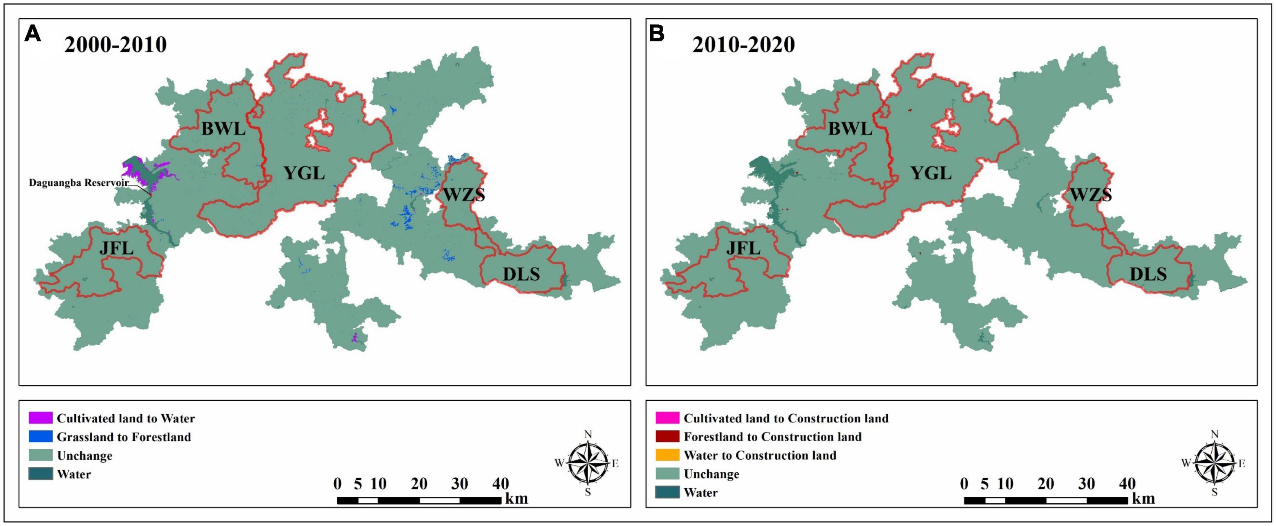
Figure 10. Spatial changes in landscape types of HTRNP. (A) Spatial changes in landscape types during 2000–2010; (B) spatial changes in landscape types during 2010–2020. JFL, Jianfengling; YGL, Yinggeling; BWL, Bawangling; WZS, Wuzhishan; DLS, Diaoluoshan.

The response of CS’s ESV to the landscape pattern changes was similar to that of WP’s ESV. Although the expansion of forestland has driven CS growth, it was insufficient to compensate for the loss of CS due to the shrinkage of cultivated land and grassland. Thus, the CS’s ESV showed a slightly decreasing trend.

The increases in areas and landscape dominance of forestland and water significantly affected HQ’s ESV. As their areas and landscape dominance increased, the landscape connectivity in HTRNP was enhanced, promoting the formation of intact habitats. Thus, the HQ’s ESV showed an increasing trend.

For HTRNP, although the decreases in cultivated land area and its LPI, grassland area and its PD led to the decrease of WP’s ESV, from a macro perspective, it reduced the water purification pressure of HTRNP. This finding is consistent with the conclusion of Xia et al. (2021). The areas and LPIs of forestland and water showed significant positive driving effects on HQ’s ESV, cultivated land area and LPI, grassland area and PD showed significant adverse inhibitory effects on HQ’s ESV. These findings are consistent with the conclusions of Dai et al. (2019) and Mandal and Chatterjee (2021).

For WS’s ESV, the increases in areas and landscape dominance of both forestland and water had adverse inhibitory effects, resulting in a decrease in WS’s ESV. This may be related to the difference in the ability of different landscape types to intercept surface runoff: the water yield of cultivated land and grassland is generally more significant than that of water and forestland because their ability to impound surface runoff is weaker than that of water and forestland (Li A. et al., 2022). Therefore, WS’s ESV tended to decrease with the conversion of cultivated land to water and grassland to forestland. In 2010, the construction of International Tourism Island in Hainan Province was officially elevated to a national strategy, converting some forestland to construction land in HTRNP (Li, 2022). For SR’s ESV, the increase in the area and the shape complexity of construction land after 2010 had a slightly significant negative inhibitory effect on SR’s ESV. However, the effect degree was limited, which may be related to its small expansion scale (Figure 10B). In addition, the increasing fragmentation of cultivated land also had a slightly significant negative inhibitory effect on the SR’s ESV, which is consistent with the conclusion of Xia et al. (2021). This may be due to the increased soil erosion caused by cultivated land fragmentation (Mitchell et al., 2015). Compared with other ESs, the factors affecting WS and SR services are more comprehensive and complex, these two ESs are not only affected by the landscape pattern changes but also related to various factors such as precipitation and topography, so the responses of these two ESVs to the landscape pattern changes were not very significant (Rao et al., 2013).

At the overall landscape level, the increase in CONTAG had a significant positive driving effect on HQ’s ESV. PD showed a negative correlation with HQ’s ESV, similar to the conclusion of Zhang et al. (2022). As the basal landscape type of HTRNP, the changes of forestland had a certain degree of guiding effect on the overall landscape pattern changes of HTRNP. As the scale, dominance, aggregation, and connectivity of the forestland have increased over the past 40 years, the aggregation and connectivity of the landscape in HTRNP have increased, which promoted the improvement of the biological HQ in the park. Due to the guiding effect of forestland’s landscape changes, the increase in CONTAG had adverse inhibitory effects on the ESVs of WP, CS, WS, and SR to varying degrees, similar to the conclusions of Ma et al. (2022).

4.2. Implications for ecosystem management in HTRNP

Rubber plantations are often an essential economic source in tropical regions of China, especially for people living near ecological reserves. However, expanding plantations may pose a potential threat to landscape connectivity. The conclusions of Liu et al. (2017) and Hu et al. (2021) for the Xishuangbanna tropical rainforest region are broadly consistent. I.e., the rapid expansion of plantations has led to a significant decline in landscape connectivity, with significant negative impacts on ESVs. The rubber industry is also one of the main economic pillars of Hainan Province, and some plantations are distributed in the HTRNP. In order to improve the economic conditions of the residents, the scales of plantations were expanded, resulting in some scattered grassland patches in the park being invaded by rubber forests. However, from the overall results, the expansion of these plantations did not significantly affect the landscape connectivity of HTRNP, which may be related to the enhancement of local ecosystem protection and the improvement of conservation methods: the five NNRs of BWL, JFL, WZS, DLS, and YGL were established successively, which further strengthened the protection of ecosystem within the scope of the reserves. Thus, even from 2000 to 2010, there were no significant changes in landscape patterns within these five NNRs (Figure 10A); “The Hainan Tropical Rainforest National Park System Pilot Program” adopted in 2019 had connected these five NNRs into a single piece, initially establishing a relatively complete HTRNP system. The implementation of these conservation policies is the main reason for the maintenance of HTRNP’s landscape connectivity. These conservation measures should be maintained and improved in the future management of the park’s ecosystems. Rubber plantation is still one of the primary economic sources to maintain the residents’ survival. Its expansion trend may continue in the short term. The areas of low importance and unavailable for wildlife in the park should be the leading site for future plantation expansion (Liu et al., 2017), and the expansion scale should be strictly restricted.

Based on the results of this study, it can be surmised that: if the cultivated land area expands in the form of large patches and the grassland area expands in the form of scattered small patches, the water purification pressure of HTRNP will increase, which is not conducive to the sustainable development of its ecosystems. For HTRNP, WP’s ESV is more suitable as a negative indicator to monitor nitrogen and phosphorus loads. As the primary source of nitrogen and phosphorus loads, controlling the cultivated land patch size within a reasonable range is necessary. We proposed to gradually convert some unproductive cultivated land into grassland or forestland, which will not only reduce the pressure of water purification in the park but also help to enhance the connectivity and integrity of grassland and forestland, thus improving the ESVs of CS and HQ; some of the retained cultivated land can be converted to increase the CS in the soil through conservation tillage with cover crops, which will also help to improve the CS’s ESV (Martín et al., 2016). In addition, controlling the conversion of cultivated land to water, reducing the size of construction land patches, and the complexity of their shapes will help to curb the decline of both WS and SR ESVs to some extent.

Hainan is a province based on ecology. The construction of HTRNP is not only one of the landmark projects of Hainan Province to promote the construction of the national ecological civilization pilot zone but also a concrete practice to explore the path of transforming clear waters and green mountains into mountains of gold and silver for realization. The monetization of ES helps people to link ES with human well-being better and raise awareness and attention to ES. In recent years, assessments on the Gross Ecosystem Product (GEP) of the HTRNP have been gradually conducted. Chen et al. (2021) conducted a preliminary assessment of the HTRNP’s GEP in 2019. In 2023, Hainan Province launched the construction of the HTRNP’s ecosystem positioning observation network system, aiming to meet the construction needs of HTRNP further. Since the HTRNP was officially selected as one of the first five national parks in China in 2021, the conservation effectiveness of the ecosystem in the park and its ES benefits have received increasing attention. This study analyzed the spatial-temporal changes of five essential ESs in HTRNP over the past 40 years. And revealed the responses of ESVs to landscape pattern changes, further complementing and improving the related studies on the HTRNP. The results can provide some references for future ecosystem management and optimization to improve the overall ES benefits of the HTRNP continuously.

4.3. Limitations and perspectives

The diversity of ES assessment methods, the subjectivity of parameter selection, and the multi-source nature of the data are the main influencing factors that lead to different ES assessment results for the same region in many studies. For example, in the CS assessment, some studies have reached different conclusions on CS services in Hainan Island, Ren et al. (2014) suggested that these differences may be related to some factors, such as the different methods of CS calculation adopted by the studies and the different carbon concentration factors used (Wang et al., 2001; Cao et al., 2002). Other ES assessments, such as WS, WP, SR, and HQ, are also affected by similar factors. In addition, there are similar problems with the ESVs’ assessments: Lei et al. (2020) used the revised unit area value equivalent factor method to assess the ESVs of Hainan Island during 1980–2018, which differed significantly from Xie et al. (2015). In this study, relevant parameters were selected and set using the relevant studies on the HTRNP and its neighboring regions as the primary reference to maximize the closeness of the assessment results to the actual situation of HTRNP. However, as the construction of the national park in China is at an initial stage, there are few studies for reference on ESs of HTRNP. The setting of relevant parameters is mainly based on studies in neighboring regions, inevitably resulting in discrepancies between the research results and the actual situation. Besides, this study used first-class landscape types to assess the ESs. The results may be slightly rough. Therefore, the landscape types of HTRNP need to be further refined in subsequent studies. For example, its landscape types can be divided into evergreen broad-leaved forests, deciduous broad-leaved forests, etc., to further explore the differences in ESs supply capacity among different plant cover types.

5. Conclusion

This study analyzed the changes of landscape patterns, ESs, and ESVs in the HTRNP during 1980–2020 and further explored the responses of ESVs to the landscape pattern changes. The results revealed that:

1. Forestland is the most dominant landscape type in HTRNP, followed by grassland. The landscape pattern changed significantly after 2000, with the conversions of cultivated land to water in the form of large patches and grassland to forestland in the form of scattered small patches, the landscape dominance and connectivity of both forestland and water increased, and the overall landscape agglomeration and connectivity tended to increase.

2. WS, WP, CS, and SR services tended to weaken, and HQ service tended to strengthen. The spatial heterogeneities of WS and SR changed significantly over time. The four ESVs of WS, HQ, SR, and CS are the main contributors to the total ESV of HTRNP. Over the past 40 years, the four ESVs of WS, WP, SR, and CS showed a decreasing trend; the HQ’s ESV tended to increase; and the total ESV tended to decrease.

3. With the transfer of some cultivated land patches and grassland patches to water and forestland in different forms, respectively, the areas and dominance of both forestland and water tended to increase, which was the main reason that HQ’s ESV tended to increase, and WP’s ESV and CS’s ESV tended to decrease. The construction land scale was relatively small, so its impacts on ESVs were limited. The responses of both WS’s ESV and SR’s ESV to the landscape pattern changes were not very significant due to topographic and climatic factors.

Data availability statement

The original contributions presented in this study are included in the article/Supplementary material, further inquiries can be directed to the corresponding author.

Author contributions

XL and HF: conceptualization and methodology. XL: software, formal analysis, and writing—original draft preparation. HF: writing—review and editing, supervision, and funding acquisition. Both authors had read and agreed to the published version of the manuscript.

Funding

This research was funded by the Hainan Provincial Natural Science Foundation of China (Grant No. 421MS015).

Conflict of interest

The authors declare that the research was conducted in the absence of any commercial or financial relationships that could be construed as a potential conflict of interest.

Publisher’s note

All claims expressed in this article are solely those of the authors and do not necessarily represent those of their affiliated organizations, or those of the publisher, the editors and the reviewers. Any product that may be evaluated in this article, or claim that may be made by its manufacturer, is not guaranteed or endorsed by the publisher.

Supplementary material

The Supplementary Material for this article can be found online at: https://www.frontiersin.org/articles/10.3389/ffgc.2023.1242068/full#supplementary-material

References

Arowolo, A. O., Deng, X., Olatunji, O. A., and Obayelu, A. E. (2018). Assessing changes in the value of ecosystem services in response to land-use/land-cover dynamics in Nigeria. Sci. Total Environ. 636, 597–609. doi: 10.1016/j.scitotenv.2018.04.277

PubMed Abstract | CrossRef Full Text | Google Scholar

Aryal, K., Maraseni, T., and Apan, A. (2022). How much do we know about trade-offs in ecosystem services? A systematic review of empirical research observations. Sci. Total Environ. 806:151229. doi: 10.1016/j.scitotenv.2021.151229

PubMed Abstract | CrossRef Full Text | Google Scholar

Ayensu, E., Van Claasen, D. R., Collins, M., Dearing, A., Fresco, L., Gadgil, M., et al. (1999). International ecosystem assessment. Science 286, 685–686.

Google Scholar

Barlow, J., França, F., Gardner, T. A., Hicks, C. C., Lennox, G. D., Berenguer, E., et al. (2018). The future of hyperdiverse tropical ecosystems. Nature 559, 517–526. doi: 10.1038/s41586-018-0301-1

PubMed Abstract | CrossRef Full Text | Google Scholar

Baude, M., Meyer, B. C., and Schindewolf, M. (2019). Land use change in an agricultural landscape causing degradation of soil based ecosystem services. Sci. Total Environ. 659, 1526–1536. doi: 10.1016/j.scitotenv.2018.12.455

PubMed Abstract | CrossRef Full Text | Google Scholar

Campbell, E. T., and Tilley, D. R. (2014). The eco-price: How environmental emergy equates to currency. Ecosyst. Serv. 7, 128–140. doi: 10.1016/j.ecoser.2013.12.002

CrossRef Full Text | Google Scholar

Cao, J., Zhang, Y., and Liu, Y. (2002). Changes in forest biomass carbon storage in Hainan Island over the last 20 years. Geogr. Res. 21, 551–560. doi: 10.11821/yj2002050003

CrossRef Full Text | Google Scholar

Cen, X. (2016). Correlation analysis and optimization between land use landscape patterns and ecosystem service values – a case study of South Coast of Hangzhou Bay. Ph.D. thesis. Hangzhou: Zhejiang University.

Google Scholar

Chen, W., Zhao, H., Li, J., Zhu, L., Wang, Z., and Zeng, J. (2020). Land use transitions and the associated impacts on ecosystem services in the Middle Reaches of the Yangtze River Economic Belt in China based on the geo-informatic Tupu method. Sci. Total Environ. 701:134690. doi: 10.1016/j.scitotenv.2019.134690

PubMed Abstract | CrossRef Full Text | Google Scholar

Chen, Z.-Z., Lei, J.-R., Wu, T.-T., Chen, D.-X., Zhou, Z., Li, Y.-L., et al. (2021). Gross ecosystem product accounting of national park: Taking Hainan Tropical Rainforest National Park as an example. J. Appl. Ecol. 32, 3883–3892. doi: 10.13287/j.1001-9332.202111.010

PubMed Abstract | CrossRef Full Text | Google Scholar

Costanza, R., d’Arge, R., De Groot, R., Farber, S., Grasso, M., Hannon, B., et al. (1997). The value of the world’s ecosystem services and natural capital. Nature 387, 253–260.

Google Scholar

Cuni-Sanchez, A., Imani, G., Bulonvu, F., Batumike, R., Baruka, G., Burgess, N. D., et al. (2019). Social perceptions of forest ecosystem services in the Democratic Republic of Congo. Hum. Ecol. 47, 839–853. doi: 10.1007/s10745-019-00115-6

CrossRef Full Text | Google Scholar

Dai, L., Li, S., Lewis, B. J., Wu, J., Yu, D., Zhou, W., et al. (2019). The influence of land use change on the spatial–temporal variability of habitat quality between 1990 and 2010 in Northeast China. J. For. Res. 30, 2227–2236. doi: 10.1007/s11676-018-0771-x

CrossRef Full Text | Google Scholar

De Groot, R., Brander, L., Van Der Ploeg, S., Costanza, R., Bernard, F., Braat, L., et al. (2012). Global estimates of the value of ecosystems and their services in monetary units. Ecosyst. Serv. 1, 50–61. doi: 10.1016/j.ecoser.2012.07.005

CrossRef Full Text | Google Scholar

Fairhead, J., Leach, M., and Scoones, I. (2012). Green grabbing: A new appropriation of nature? J. Peasant Stud. 39, 237–261.

Google Scholar

Fan, Z., and Li, W. (2020). Research on the realization mechanism of ecological product value-a case study of Guizhou Province. J. Hebei Geo. Univ. 43, 82–90. doi: 10.3390/ijerph19105892

PubMed Abstract | CrossRef Full Text | Google Scholar

Fang, F., Chen, Y., Liang, J., and Fu, X. (2013). Construction benefit evaluation of coastal shelter forest system in Hainan province. J. Central South Univ. For. Technol. 33, 115–119. doi: 10.1016/j.ecolind.2022.109119

CrossRef Full Text | Google Scholar

Fang, Z., Bai, Y., Jiang, B., Alatalo, J. M., Liu, G., and Wang, H. (2020). Quantifying variations in ecosystem services in altitude-associated vegetation types in a tropical region of China. Sci. Total Environ. 726:138565. doi: 10.1016/j.scitotenv.2020.138565

PubMed Abstract | CrossRef Full Text | Google Scholar

Ge, Y. (2020). Evolution and optimization of green space pattern in the second green belt of beijing municipality area based on ecosystem services evaluation. Ph.D. thesis. Beijing: Beijing Forestry University.

Google Scholar

Gong, W., Duan, X., Sun, Y., Zhang, Y., Ji, P., Tong, X., et al. (2022). Multi-scenario simulation of land use/cover change and carbon storage assessment in Hainan coastal zone from perspective of free trade port construction. J. Clean. Prod. 12:135630. doi: 10.1016/j.jclepro.2022.135630

CrossRef Full Text | Google Scholar

Guo, Z., Xiao, X., Gan, Y., and Zheng, Y. (2001). Ecosystem functions, services and their values–a case study in Xingshan County of China. Ecol. Econ. 38, 141–154. doi: 10.1016/S0921-8009(01)00154-9

CrossRef Full Text | Google Scholar

Guswa, A. J., Brauman, K. A., Brown, C., Hamel, P., Keeler, B. L., and Sayre, S. S. (2014). Ecosystem services: Challenges and opportunities for hydrologic modeling to support decision making. Water Resour. Res. 50, 4535–4544. doi: 10.1002/2014WR015497

CrossRef Full Text | Google Scholar

Han, N., Yu, M., and Jia, P. (2022). Multi-scenario landscape ecological risk simulation for sustainable development goals: A case study on the central mountainous area of Hainan Island. Int. J. Environ. Res. Public Health 19:4030. doi: 10.3390/ijerph19074030

PubMed Abstract | CrossRef Full Text | Google Scholar

Hernández-Morcillo, M., Plieninger, T., and Bieling, C. (2013). An empirical review of cultural ecosystem service indicators. Ecol. Indic. 29, 434–444. doi: 10.1016/j.ecolind.2013.01.013

CrossRef Full Text | Google Scholar

Hoang, N. T., and Kanemoto, K. (2021). Mapping the deforestation footprint of nations reveals growing threat to tropical forests. Nat. Ecol. Evol. 5, 845–853. doi: 10.1038/s41559-021-01417-z

PubMed Abstract | CrossRef Full Text | Google Scholar

Hou, L., Wu, F., and Xie, X. (2020). The spatial characteristics and relationships between landscape pattern and ecosystem service value along an urban-rural gradient in Xi’an city, China. Ecol. Indic. 108:105720. doi: 10.1016/j.ecolind.2019.105720

CrossRef Full Text | Google Scholar

Hu, Z., Yang, X., Yang, J., Yuan, J., and Zhang, Z. (2021). Linking landscape pattern, ecosystem service value, and human well-being in Xishuangbanna, southwest China: Insights from a coupling coordination model. Glob. Ecol. Conserv. 27:e01583. doi: 10.1016/j.gecco.2021.e01583

CrossRef Full Text | Google Scholar

Kemkes, R. J., Farley, J., and Koliba, C. J. (2010). Determining when payments are an effective policy approach to ecosystem service provision. Ecol. Econ. 69, 2069–2074. doi: 10.1016/j.ecolecon.2009.11.032

CrossRef Full Text | Google Scholar

Kertész, Á, Nagy, L. A., and Balázs, B. (2019). Effect of land use change on ecosystem services in Lake Balaton Catchment. Land Use Policy 80, 430–438. doi: 10.1007/s42977-020-00032-6

PubMed Abstract | CrossRef Full Text | Google Scholar

Kroeger, T., and Casey, F. (2007). An assessment of market-based approaches to providing ecosystem services on agricultural lands. Ecol. Econ. 64, 321–332. doi: 10.1016/j.ecolecon.2007.07.021

CrossRef Full Text | Google Scholar

Kubiszewski, I., Costanza, R., Anderson, S., and Sutton, P. (2020). “The future value of ecosystem services: Global scenarios and national implications,” in Environmental assessments, ed. K. N. Ninan (Cheltenham: Edward Elgar Publishing). doi: 10.1016/j.ecoser.2017.05.004

CrossRef Full Text | Google Scholar

Lawler, J. J., Lewis, D. J., Nelson, E., Plantinga, A. J., Polasky, S., Withey, J. C., et al. (2014). Projected land-use change impacts on ecosystem services in the United States. Proc. Natl. Acad. Sci. U.S.A. 111, 7492–7497.

Google Scholar

Legendre, P. (2008). Studying beta diversity: Ecological variation partitioning by multiple regression and canonical analysis. J. Plant Ecol. 1, 3–8.

Google Scholar

Lei, J., Chen, Z., Chen, X., Li, Y., and Wu, T. (2020). Spatio-temporal changes of land use and ecosystem services value in Hainan Island from 1980 to 2018. Acta Ecol. Sin. 40, 4760–4773. doi: 10.1093/jpe/rtm001

CrossRef Full Text | Google Scholar

Lei, J.-R., Chen, Y.-Q., Chen, Z.-Z., Chen, X.-H., Wu, T.-T., and Li, Y.-L. (2022). Spatiotemporal evolution of habitat quality in three basins of Hainan Island based on InVEST model. J. Appl. Ecol. 33, 2511–2520. doi: 10.13287/j.1001-9332.202209.019

PubMed Abstract | CrossRef Full Text | Google Scholar

Li, A., Ye, C., Zhu, L., Wang, Y., Liang, X., and Zou, Y. (2022). Impact from land use/land cover change on function of water yield service: A case study on National Park of Hainan Tropical Rainforest. Water Resour. Hydropower Eng. 53, 36–45. doi: 10.3389/ffgc.2023.1131264/full

CrossRef Full Text | Google Scholar

Li, C., Zhao, J., Zhuang, Z., and Gu, S. (2022). Spatiotemporal dynamics and influencing factors of ecosystem service trade-offs in the Yangtze River Delta urban agglomeration. Acta Ecol. Sin. 14, 1–13. doi: 10.3390/land12040929

CrossRef Full Text | Google Scholar

Li, J., Zhou, K., Xie, B., and Xiao, J. (2021). Impact of landscape pattern change on water-related ecosystem services: Comprehensive analysis based on heterogeneity perspective. Ecol. Indic. 133:108372. doi: 10.1016/j.ecolind.2021.108372

CrossRef Full Text | Google Scholar

Li, L. (2022). Analysis of landscape pattern and spatio-temporal change for ecosystem service value in Hainan tropical rain Forest National Park. Ph.D. thesis. Hainan: Hainan University.

Google Scholar

Li, L., Tang, H., Lei, J., and Song, X. (2022). Spatial autocorrelation in land use type and ecosystem service value in Hainan Tropical Rain Forest National Park. Ecol. Indic. 137:108727. doi: 10.1016/j.ecolind.2022.108727

CrossRef Full Text | Google Scholar

Liu, J., Chen, Q., Peng, Y., and Hu, X. (2009). Forest ecosystem services and their valuation in the central mountainous areas of Hainan. Ecol. Econ. 2, 24–30.

Google Scholar

Liu, P., Li, W., Yu, Y., Tang, R., Guo, X., Wang, B., et al. (2019). How much will cash forest encroachment in rainforests cost? A case from valuation to payment for ecosystem services in China. Ecosyst. Serv. 38:100949. doi: 10.1016/j.ecoser.2019.100949

CrossRef Full Text | Google Scholar

Liu, Q., Yang, D., Cao, L., and Anderson, B. (2022). Assessment and prediction of carbon storage based on land use/land cover dynamics in the tropics: A case study of Hainan Island, China. Land 11:244. doi: 10.3390/land11020244

CrossRef Full Text | Google Scholar

Liu, S., Yin, Y., Liu, X., Cheng, F., Yang, J., Li, J., et al. (2017). Ecosystem Services and landscape change associated with plantation expansion in a tropical rainforest region of Southwest China. Ecol. Model. 353, 129–138. doi: 10.1016/j.ecolmodel.2016.03.009

CrossRef Full Text | Google Scholar

Loomisa, J., Kentb, P., Strangec, L., Fauschc, K., and Covichc, A. (2018). “Measuring the total economic value of restoring ecosystem services in an impaired river basin: Results from a contingent valuation survey,” in Economics of water resources, eds A. Dinar and Y. Tsur (London: Routledge).

Google Scholar

Ma, S., Wang, L. J., Wang, H. Y., Zhang, X., and Jiang, J. (2022). Spatial heterogeneity of ecosystem services in response to landscape patterns under the Grain for Green Program: A case-study in Kaihua County, China. Land Degrad. Dev. 33, 1901–1916. doi: 10.1002/ldr.4272

CrossRef Full Text | Google Scholar

Mandal, M., and Chatterjee, N. D. (2021). Spatial alteration of fragmented forest landscape for improving structural quality of habitat: A case study from Radhanagar Forest Range, Bankura District, West Bengal, India. Geol. Ecol. Landsc. 5, 252–259.

Google Scholar

Martín, J. R., Álvaro-Fuentes, J., Gonzalo, J., Gil, C., Ramos-Miras, J. J., Corbí, J. G., et al. (2016). Assessment of the soil organic carbon stock in Spain. Geoderma 264, 117–125. doi: 10.1016/j.geoderma.2015.10.010

CrossRef Full Text | Google Scholar

Millennium Ecosystem Assessment (2005). Ecosystems and human well-being, Vol. 5. Washington, DC: Island press.

Google Scholar

Mitchell, M. G., Suarez-Castro, A. F., Martinez-Harms, M., Maron, M., McAlpine, C., Gaston, K. J., et al. (2015). Reframing landscape fragmentation’s effects on ecosystem services. Trends Ecol. Evol. 30, 190–198. doi: 10.1016/j.tree.2015.01.011

PubMed Abstract | CrossRef Full Text | Google Scholar

Navrud, S., and Strand, J. (2018). Valuing global ecosystem services: What do European experts say? Applying the Delphi method to contingent valuation of the Amazon rainforest. Environ. Resour. Econ. 70, 249–269. doi: 10.1007/s10640-017-0119-6

CrossRef Full Text | Google Scholar

Piponiot, C., Rutishauser, E., Derroire, G., Putz, F. E., Sist, P., West, T. A., et al. (2019). Optimal strategies for ecosystem services provision in Amazonian production forests. Environ. Res. Lett. 14:124090.

Google Scholar

Qi, W., Li, H., Zhang, Q., and Zhang, K. (2019). Forest restoration efforts drive changes in land-use/land-cover and water-related ecosystem services in China’s Han River basin. Ecol. Eng. 126, 64–73.

Google Scholar

Rao, E., Xiao, Y., Ouyang, Z., and Zheng, H. (2013). Spatial characteristics of soil conservation service and its impact factors in Hainan Island. Acta Ecol. Sin. 33, 746–755.

Google Scholar

Rao, E., Xiao, Y., Ouyang, Z., and Zheng, H. (2016). Changes in ecosystem service of soil conservation between 2000 and 2010 and its driving factors in southwestern China. Chin. Geogr. Sci. 26, 165–173.

Google Scholar

Ren, H., Li, L., Liu, Q., Wang, X., Li, Y., Hui, D., et al. (2014). Spatial and temporal patterns of carbon storage in forest ecosystems on Hainan island, southern China. PLoS One 9:e108163. doi: 10.1371/journal.pone.0108163

PubMed Abstract | CrossRef Full Text | Google Scholar

Salzman, J., Bennett, G., Carroll, N., Goldstein, A., and Jenkins, M. (2018). The global status and trends of payments for ecosystem services. Nat. Sustain. 1, 136–144.

Google Scholar

Schröter, M., Ring, I., Schröter-Schlaack, C., and Bonn, A. (2019). “The ecosystem service concept: Linking ecosystems and human wellbeing,” in Atlas of ecosystem services, eds M. Schröter, A. Bonn, S. Klotz, R. Seppelt, and C. Baessler (Berlin: Springer), 7–11.

Google Scholar

Sharp, R., Tallis, H., Ricketts, T., Guerry, A. D., Wood, S. A., Chaplin-Kramer, R., et al. (2016). InVEST+ VERSION+ User’s guide. The natural capital project. Stanford: Stanford University.

Google Scholar

Sheng, L., Jin, Y., and Huang, J. (2010). Value estimation of conserving water and soil of ecosystems in China. J. Nat. Resour 25, 1105–1113.

Google Scholar

Sun, X., Li, S., Yu, J., Fang, Y., Zhang, Y., and Cao, M. (2019). Evaluation of ecosystem service value based on land use scenarios: A case study of Qianjiangyuan National Park pilot. Biodivers. Sci. 27, 51–63.

Google Scholar

Tallis, H., and Kareiva, P. (2005). Ecosystem services. Curr. Biol. 15, R746–R748.

Google Scholar

Tallis, H., and Polasky, S. (2009). Mapping and valuing ecosystem services as an approach for conservation and natural-resource management. Ann. N. Y. Acad. Sci. 1162, 265–283.

Google Scholar

Turner, M. G. (1987). Spatial simulation of landscape changes in Georgia: A comparison of 3 transition models. Landsc. Ecol. 1, 29–36.

Google Scholar

Wang, L., Xiao, Y., Ouyang, Z., Wei, Q., Bo, W., Zhang, J., et al. (2017). Gross ecosystem product accounting in the national key ecological function area. China Popul. Resour. Environ. 27, 146–154. doi: 10.13287/j.1001-9332.202111.017

PubMed Abstract | CrossRef Full Text | Google Scholar

Wang, X., Feng, Z., and Ouyang, Z. (2001). Vegetation carbon storage and density of forest ecosystems in China. J. Appl. Ecol. 12, 13–16. doi: 10.1186/s40663-019-0210-2

PubMed Abstract | CrossRef Full Text | Google Scholar

Wang, X., Wang, X., Zhu, M., Wang, W., Liang, Q., Zou, Y., et al. (2017). Carbon storage and economic assessment of the main forest types vegetation in Hainan. J. Central South Univ. For. Technol. 37, 92–98. doi: 10.3390/land11020244

CrossRef Full Text | Google Scholar

Wang, Y., Li, X., Zhang, Q., Li, J., and Zhou, X. (2018). Projections of future land use changes: Multiple scenarios-based impacts analysis on ecosystem services for Wuhan city, China. Ecol. Indic. 94, 430–445. doi: 10.1016/j.ecolind.2018.06.047

CrossRef Full Text | Google Scholar

Wang, Z., Mao, D., Li, L., Jia, M., Dong, Z., Miao, Z., et al. (2015). Quantifying changes in multiple ecosystem services during 1992–2012 in the Sanjiang Plain of China. Sci. Total Environ. 514, 119–130. doi: 10.1016/j.scitotenv.2015.01.007

PubMed Abstract | CrossRef Full Text | Google Scholar

Watson, J. E., Evans, T., Venter, O., Williams, B., Tulloch, A., Stewart, C., et al. (2018). The exceptional value of intact forest ecosystems. Nat. Ecol. Evol. 2, 599–610. doi: 10.1038/s41559-018-0490-x

PubMed Abstract | CrossRef Full Text | Google Scholar

Williams, J. R. (1995). “The EPIC model,” in Computer models of watershed hydrology, ed. V. P. Singh (Denver, CO: Highlands Ranch).

Google Scholar

Xia, H., Kong, W., Zhou, G., and Sun, O. J. (2021). Impacts of landscape patterns on water-related ecosystem services under natural restoration in Liaohe River Reserve, China. Sci. Total Environ. 792:148290. doi: 10.1016/j.scitotenv.2021.148290

PubMed Abstract | CrossRef Full Text | Google Scholar

Xia, H., Yuan, S., and Prishchepov, A. V. (2023). Spatial-temporal heterogeneity of ecosystem service interactions and their social-ecological drivers: Implications for spatial planning and management. Resour. Conserv. Recycl. 189:106767.

Google Scholar

Xiao, H. (1999). Spatial distribution characteristics of soil erosion in Hainan Island by GIS. Res. Environ. Sci. 5, 75–80.

Google Scholar

Xiao, Q., Xiao, Y., Ouyang, Z. Y., Xu, W. H., Xiang, S., and Li, Y. Z. (2014). Value assessment of the function of the forest ecosystem services in Chongqing. Acta Ecol. Sin. 34, 216–223.

Google Scholar

Xie, G., Zhang, C., Zhang, C., Xiao, Y., and Lu, C. (2015). The value of ecosystem services in China. Resour. Sci. 37, 1740–1746. doi: 10.1007/BF02886190

CrossRef Full Text | Google Scholar

Xu, X., Liu, J., Zhang, S., Li, R., Yan, C., and Wu, S. (2018). China’s multi-period land use land cover remote sensing monitoring data set (CNLUCC). Beijing: Resource and Environment Data Cloud Platform.

Google Scholar

Yang, Y., Li, M., Feng, X., Yan, H., Su, M., and Wu, M. (2021). Spatiotemporal variation of essential ecosystem services and their trade-off/synergy along with rapid urbanization in the Lower Pearl River Basin, China. Ecol. Indic. 133:108439. doi: 10.1016/j.ecolind.2021.108439

CrossRef Full Text | Google Scholar

Yao, X., Zhou, L., Wu, T., and Ren, M. (2022). Landscape dynamics and ecological risk of the expressway crossing section in the Hainan Rainforest National Park. Acta Ecol. Sin. 42, 6695–6703. doi: 10.3390/land12061114

CrossRef Full Text | Google Scholar

Yu, B., Rao, E., Chao, X., Shi, J., Zhang, C., Xu, W., et al. (2016). Evaluating the effectiveness of nature reserves in soil conservation on Hainan Island. Acta Ecol. Sin. 36, 3694–3702. doi: 10.3390/f14071293

PubMed Abstract | CrossRef Full Text | Google Scholar

Yu, M., Jin, H., and Li, Q. (2020). Gross ecosystem product (GEP) accounting for Chenggong District. J. West China For. Sci 49, 41–55.

Google Scholar

Yushanjiang, A., Zhang, F., and Yu, H. (2018). Quantifying the spatial correlations between landscape pattern and ecosystem service value: A case study in Ebinur Lake Basin, Xinjiang, China. Ecol. Eng. 113, 94–104. doi: 10.1016/j.ecoleng.2018.02.005

CrossRef Full Text | Google Scholar

Zhang, D., Wang, J., Wang, Y., Xu, L., Zheng, L., Zhang, B., et al. (2022). Is there a spatial relationship between urban landscape pattern and habitat quality? Implication for landscape planning of the yellow river basin. Int. J. Environ. Res. Public Health 19:11974. doi: 10.3390/ijerph191911974

PubMed Abstract | CrossRef Full Text | Google Scholar

Zhang, K., Shu, A., Xu, X., Yang, Q., and Yu, B. (2008). Soil erodibility and its estimation for agricultural soils in China. J. Arid Environ. 72, 1002–1011. doi: 10.1016/j.jaridenv.2007.11.018

CrossRef Full Text | Google Scholar

Zhang, W., and Fu, J. (2003). Rainfall erosivity estimation under different rainfall amount. Resour. Sci. 25, 35–41.

Google Scholar

Zhe, W., Xin, C., Beibei, L., Jinfeng, C., and Lixu, P. (2013). Risk assessment of nitrogen and phosphorus loads in Hainan Island based on InVEST model. Chin. J. Trop. Crops 34, 1791–1797. doi: 10.3390/su142114344

CrossRef Full Text | Google Scholar

Zheng, H., Wang, L., Peng, W., Zhang, C., Li, C., Robinson, B. E., et al. (2019). Realizing the values of natural capital for inclusive, sustainable development: Informing China’s new ecological development strategy. Proc. Natl. Acad. Sci. U.S.A. 116, 8623–8628. doi: 10.1073/pnas.1819501116

PubMed Abstract | CrossRef Full Text | Google Scholar