Evaluating climate change impacts on ecosystem resources through the lens of climate analogs

Introduction

The direct and indirect impacts from ongoing climate change are being observed throughout social and ecological systems across the globe (Pörtner et al., 2022). Recent studies have documented the susceptibility of dominant forest vegetation to current and predicted future climate and suggest that dominant vegetation types across portions of their range are unlikely to persist over time (Dobrowski et al., 2011; Coop et al., 2020; Hill et al., 2023). Declines in conifer forests across 30% of the southern Sierra region in California have been recorded following recent natural disturbances leaving vast areas susceptible to conversions to alternative vegetation types (Steel et al., 2022). As disturbances from drought, insect outbreaks, and wildfires increase in extent and severity, ecological impacts will be more apparent where pre-fire vegetation types are currently outside their climatic tolerances (Thorne et al., 2017; Triepke et al., 2019; Coop et al., 2020; Hill et al., 2023).

Social-ecological systems are inherently multi-dimensional and changes in dominant climate regimes will likely permeate across biotic and abiotic processes Manley et al. (This issue). Tracking direct and indirect impacts from climate change is a high-dimensional problem, and understanding how climate may change in a given area may not adequately inform potential changes to key ecosystem provisions such as carbon sequestration, fire dynamics, or biodiversity (Garcia et al., 2014). The direction and degree of these impacts may vary among ecosystem resources and impacts will likely vary spatially across biophysical gradients (Thorne et al., 2017).

While land mangers acknowledge the threats imposed by climate change, many barriers exist towards integrating climate change impacts into management planning (Urgenson et al., 2017; Morecroft et al., 2019; Brice et al., 2020). The ability to anticipate the magnitude and direction of change in key ecosystem properties can help managers strategically plan appropriate place-based treatments (Stein et al., 2014). Treatments are aimed at either preventing transitions to alternative states by increasing the adaptive capacity of an ecosystem, or facilitating the transition to desirable alternative states that are more suited to predicted future climates (Coop et al., 2020; Schuurman et al., 2020). Such goals represent a paradigm shift in management from a resistance-based model aimed at preventing change, towards managing for change and including a broader set of objectives that acknowledge the non-stationary nature of ecosystems over space and time (Aplet and Cole, 2010; Stein et al., 2014; McWethy et al., 2019). However, managers require tools to help reduce uncertainty in future climate conditions and associated downstream effects on key ecosystem resources to achieve these broader goals. Such information can help gain a shared understanding among stakeholders and policymakers of the potential impediments that climate may pose on securing and sustaining resources (Grafton et al., 2019; Gaines et al., 2022). Such models need to be scalable to meet the needs of large regional landscapes, adaptable to various geographies and ecosystem resources, of high resolution to inform project-level planning, and easily integrated into decision support and other management planning tools to allow for integration into the planning process.

Climate analog modeling is one such approach that uses a space-for-time substitution to identify locations across a large geographic region that match the climate regime of a given focal cell (Williams et al., 2007; Mahony et al., 2017). Specifically, backwards or reverse climate analogs are used to answer the question, “where on the landscape do climate regimes exist today that match my future predicted climate conditions?” Such analyzes have been used to infer 1) the occurrence and ubiquity of future climates currently on the landscape (Williams et al., 2007; Mahony et al., 2018), 2) the distance between a focal cell and its future climate match (Dobrowski and Parks, 2016), 3) the displacement potential of climates outside of protected natural areas (Dobrowski et al., 2021; Parks et al., 2023), and 4) the likelihood of changes in key ecosystem properties under future climate change (Parks et al., 2018, 2019; Hoecker et al., 2023). In the latter example, Parks et al. (2018) used climate analog modeling to quantify climate susceptibility by comparing dominant vegetation and associated fire regime conditions at each focal cell to their respective climate analog locations.

The objectives of the current study were to extend the methods of previous climate analog studies and incorporate them into a multi-resource ecosystem assessment of future potential conditions across California. Current resource conditions were modeled against their analog counterparts to determine the magnitude and direction of change anticipated under mid-21^st century climate using fuzzy logic. This allowed for the integration of model outputs to assess potential climate impacts across a spectrum of ecological resources. From these results we asked the following questions: What are the patterns of future resource stability and are there similarities in the patterns across ecosystem resources? What are the biophysical factors driving patterns of future resource stability? How do inferences about resource stability differ using climate velocity (e.g., distance to climate analogs) versus the functional assessment used here?

Materials and methods

Study area

Our study was motivated by California’s Wildfire and Forest Resilience Action Plan and the associated Task Force that is aimed at developing strategies to increase the pace and scale of management across the Sate (California Wildfire and Forest Resilience Task Force, 2022). Accordingly, we applied our modeling framework to 1 km cells across the state of California, United States (Figure 1). Some analysis results were summarized to the six broad ecoregions established by the Task Force, which included: Sierra, North Coast, Central Coast, South Coast, Central Valley, and Basin and Range regions (Figure 1).

FIGURE 1

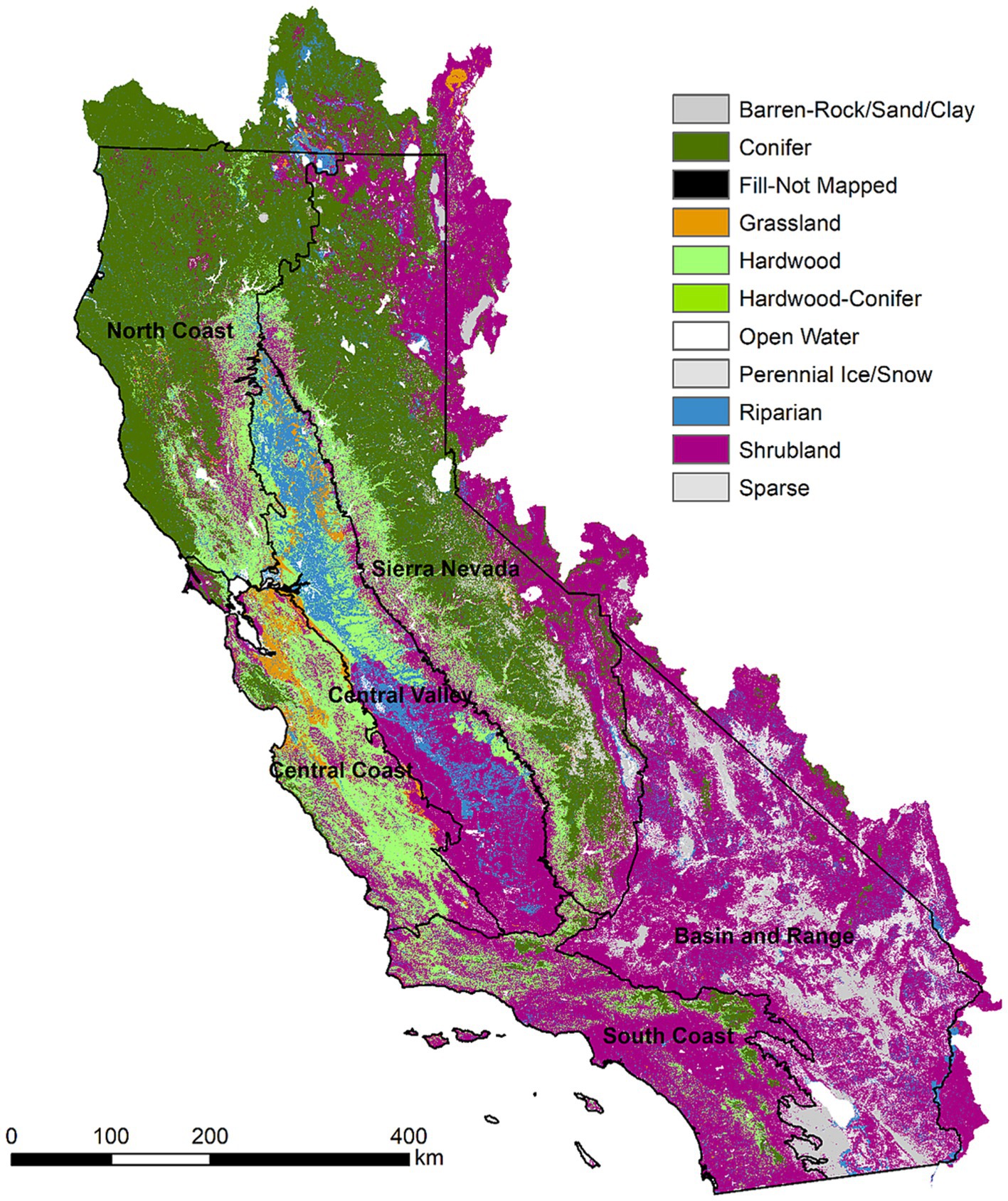
Figure 1. Ecoregions of the state of California and LANDFIRE Biophysical Setting (BpS) GROUPVEG classification representing potential vegetation under a pre-European settlement disturbance regime.

Modeling workflow

We provide a detailed description of the modeling components in the following sections, and a graphical workflow is presented in Figure 2. In summary, for each 1 km cell in California, the process began by projecting climate to mid-century and identifying locations with similar climate regimes on the landscape today (i.e., climate analogs). Data at each analog location were collected across six ecosystem resources (e.g., vegetation, wildfire, biodiversity) and compared to each cell in California using fuzzy logic to determine the degree of resource stability under climate change (Figure 2).

FIGURE 2

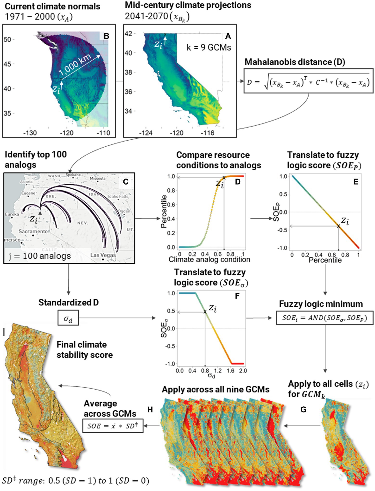
Figure 2. Example modeling workflow outlining the methods behind the climate analog modeling for each 1 km cell in California [ $z_i$ ; (A–C)], subsequent fuzzy logic modeling (D–F), extrapolation across cells and climate models (G,H), and combining results into a final map (I). See Supplementary Figures S1-S7 for more information on the specific logic model details, which vary across the six ecosystem resources. Supplementary Figure S8 provides the logic for averaging across GCMs (Steps H-I).

Climate analog modeling

We followed Mahony et al. (2017) and others (e.g., Dobrowski et al., 2021) who developed and applied methods to statistically evaluate climatic similarity across large regions using a backwards or reverse climate analog approach. For a given focal cell, reverse analog modeling identifies locations across a broad geography that currently have a climate regime similar to the future climate projected for the focal cell (Hamann et al., 2015).

Selection of climate analog locations

We used the Mahalanobis distance (D) and the standardization based on the Chi distribution (σ; see, Mahony et al., 2017) as the measure of statistical distance between 1) mid-21^st century (2041–2070) climate for all focal cells within California and 2) recent (reference) climate conditions (1971–2000) for selected analog cells within a 1,000 km radius. The Mahalanobis calculation requires an estimate of the sample inverse covariance matrix (ICV) for the climate data. We used the distribution of future climate data as a conservative approach to estimating the ICV. These data 1) exhibited larger variation compared to the reference climate data, 2) likely overestimated the variability, and 3) led to a more conservative estimate of climate distance (C. R. Mahony, personal communication).

For each focal cell, we identified the top 100 climate analogs with the lowest σ value. The selection of the 1,000 km buffer was necessary to limit processing run times while ensuring an adequate search window. Dobrowski et al. (2021) used a 2000 km buffer for identifying analogs for the end-of-21st century climate projections. Parks et al. (2023) used a 500 km radius for mid-21st century based on the estimated upper range of dispersal for some species. Schloss et al. (2012) reported a 15 km yr⁻¹ upper quantile estimate of dispersal velocity, which matches the 1,000 km search window used here.

The selection of climate analog locations was done separately for each of nine downscaled general circulation models (GCM). These GCMs were found to be most representative of spatial variation in model uncertainty and were recommended for use in regional analyzes (Mahony et al., 2022). GCMs included: ACCESS-ESM1-5, CNRM-ESM2-1, EC-Earth3, GFDL-ESM4, GISS-E2-1-G, MIROC6, MPI-ESM1-2-HR, MRI-ESM2-0, UKEMS1-0-LL. This resulted in the identification of a total of 900 climate analogs for each 1 km cell in California. Project climate data were from the Representative Concentration Pathway (RCP) 8.5 and Shared Socioeconomic Pathway (SSP) 5 Fossil Fuel Development from the 6th Coupled Model Intercomparison Project Phases (CMIP6) to match previous studies (Dobrowski and Parks, 2016; Parks et al., 2018; Dobrowski et al., 2021). All computations were done within the R version v4.04 computing environment (R Core Team, 2021).

Climate data

ClimateNA (v7.30, Wang et al., 2016) data were used to represent both current climate (reference climate data for the years 1971–2000) and mid-21st century projected climate (years 2041–2070). We selected the reference time period to balance the representation of climate prior to major warming (sensu, Dobrowski et al., 2021) while still representing more recent climate conditions to support the assessment of “current conditions” (see also Parks et al., 2019). The mid-21st century future time period was chosen as it was relevant for management planning horizons while still representing a period of significant future climate change. ClimateNA downscales gridded climate data from PRISM (Daly et al., 2000; Daly and Bryant, 2013) and WorldClim (Fick and Hijmans, 2017) for historical and current time periods and Coupled Model Intercomparison Project (CMIP6) for projected future conditions. The climateNA model downscales gridded climate data from 4 km to scale-free point data using a combination of bilinear interpolation between cell centers and local elevation adjustments using empirical lapse rates specific to the climate variable, location, and elevation (Wang et al., 2016). These data have been used in previous climate analog modeling efforts (Littlefield et al., 2017; Mahony et al., 2017; Parks et al., 2018, 2019).

Variable selection

As Mahony et al. (2017) point out, the selection of the number of variables to represent climate conditions requires a balance between generality (too few variables) and specificity (too many variables). Parks et al. (2018) developed climate analog models for the western US using two variables to represent climate: Hargreaves’ climatic moisture deficit (CMD; mm yr.⁻¹) and Hargreaves’ reference evaporation minus climatic moisture deficit (i.e., evapotranspiration [ET; mm yr.⁻¹]). Williams et al. (2007) used four climate variables: mean summer temperature, mean winter temperature, summer precipitation, and winter precipitation. For this study, we conducted initial tests using different selections and numbers of climate variables. In general, given the high collinearity of the ClimateNA variables, the model was robust to the climate variables selected, but sensitive to the number of variables. As such, we selected a series of five climate variables that were similar to variables used across previous studies and represented both seasonal temperature and moisture regimes to reflect climate gradients and main drivers of ecosystem processes. The final set included: climatic moisture deficit ( $CMD$ ), summer precipitation ( $PP{T}_{sm}$ ), winter precipitation $\left(PP{T}_{\mathit{wt}}\right)$ , mean warmest month temperature ( $\mathit{MWMT}$ ), mean coldest month temperature ( $\mathit{MCMT}$ ).

Evaluating ecosystem resource stability under climate change

We used fuzzy logic to evaluate future resource stability (FRS) across six main ecosystem resource outcomes, which encompass a wide array of essential ecosystem services. Fuzzy logic has been used widely in spatial decision support applications as a means of evaluating environmental conditions and informing strategic and tactical planning (Reynolds, 2001; Reynolds et al., 2023). Logic models interpret data to determine the degree to which they satisfy a proposition (e.g., forest vegetation is resilient to climate change). Relevant to the current application, fuzzy logic evaluates the condition of spatial data using one or more membership functions (Supplementary Figures S1–S8) (Reynolds, 2001). Outputs from fuzzy logic modeling are strength of evidence (SOE) scores that quantify the level of support towards accepting the proposition that a given resource is stable under mid-century climate. SOE scores range from −1.0 (low resource stability) to +1.0 (high resource stability).

The selected ecosystem resources were based on six of the ten Pillars from the Framework for Resilience (Manley et al., This issue), which is a hierarchical conceptual model used to characterize the many interrelated social and ecological functions provided by resilient ecosystems. Pillars represent ecosystem service outputs expected from resilient systems and are often the target of management. For each ecosystem resource (aka Pillar), we developed a logic model to evaluate the proposition that a given resource will maintain or improve in condition under climate change (e.g., live carbon will not decrease under climate change) (Table 1; Supplementary Figures S1–S7).

TABLE 1

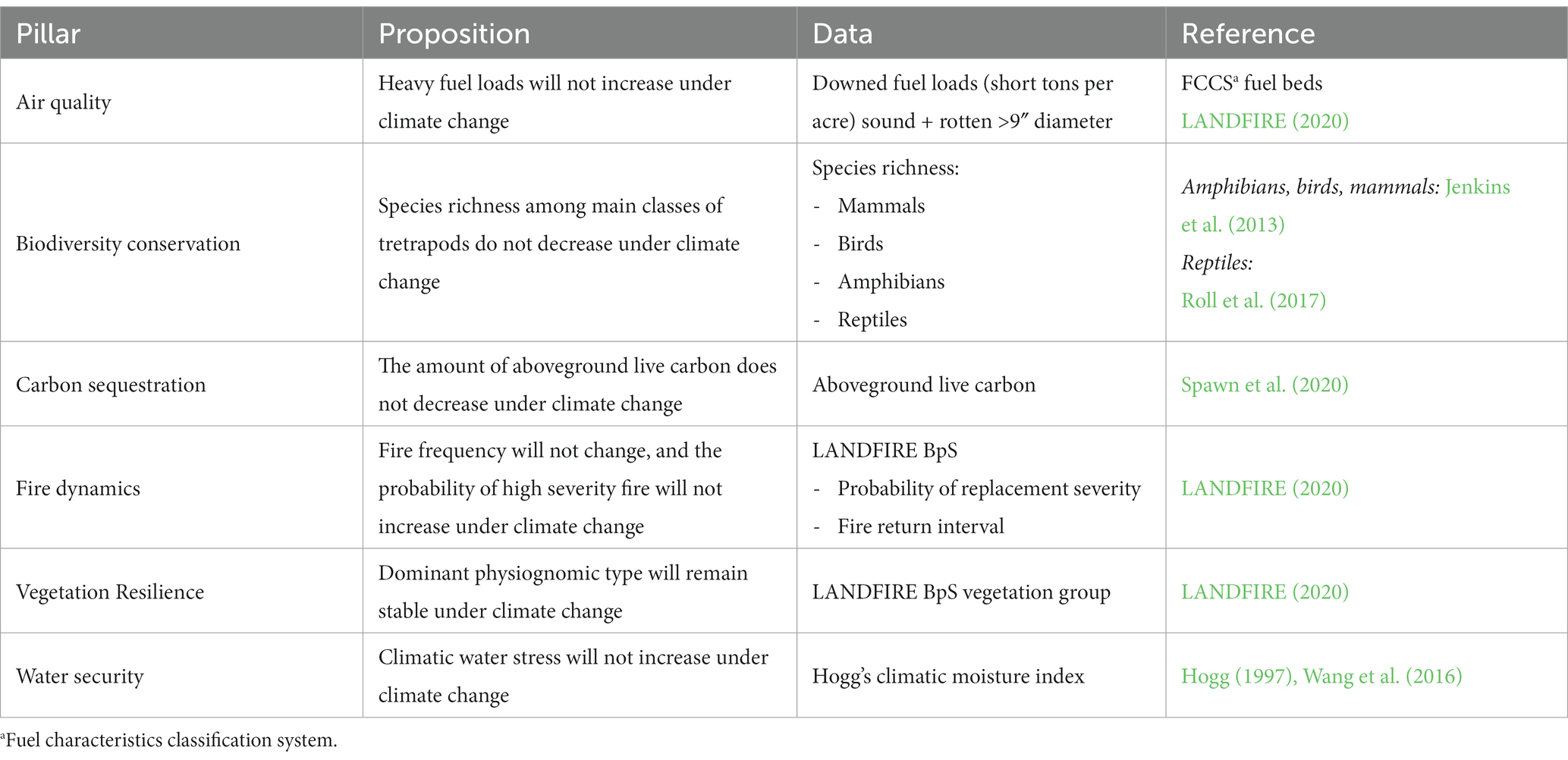
Table 1. Future condition evaluations using fuzzy logic and climate analog modeling.

The fuzzy logic model for each ecosystem resource consisted of two terms. First, the standardized Mahalanobis σ score (see below) represented the degree of climatic matching between each analog and the focal cell, referred to as the Analog Similarity Score. Second, we compared the current resource conditions at the focal cell with those across a set of 900 climate analog locations, referred to as the Ecological Score. These two scores were calculated for each focal cell, and the score with the lowest value (poorest strength of evidence) was assigned to the cell for each GCM.

Focal cell scores for the individual GCM models (n = 9) were combined to derive a final resource stability score. The SOE scores were first averaged across the nine GCM models, and then the standard deviation of the SOE scores was scaled from 1 (no variation among GCMs, $\mathit{SO}{E}_{SD}=0$ ) to 0.5 (high variation among GCMs $\mathit{SO}{E}_{SD}=1$ ). The SOE and $\mathit{SO}{E}_{SD}$ scores were multiplied together, which served to temper the strength of the resource stability score in instances of high variability in logic model scores across the GCMs (Supplementary Figure S8).

Analog similarity score

The comparison of focal and analog climatic conditions was conducted once to derive the Analog Similarity Score. We used the Mahalanobis standardized σ as a measure of climatic dissimilarity between the future climate of a given focal cell and its top 100 climate analogs. The σ statistic is similar to a Z-score with lower scores indicating more similar climate matches. Dobrowski et al. (2021) suggested that analogs with > $2$ σ indicated a poor climate match and represented a novel or no-analog future climate condition. Parks et al. (2022) used a < 0.5σ cutoff to indicate good climate matches. From these examples, we used a > 1.64σ to indicate poor climate matches (SOE = −1) and < 0.5σ as good climate matches (SOE = +1) (Supplementary Figure S1). Intermediate values of ${\sigma }_d$ were linearly ramped between −1 and + 1.

Vegetation Resilience FRS calculation

We evaluated the likelihood and severity of dominant vegetation conversions under climate change to represent the Vegetation Resilience Ecological Score. We followed the methods of Parks et al. (2018), who used LANDFIRE biophysical setting (BpS; LANDFIRE, 2020) data to compare vegetation among focal cells and their respective climate analogs. The BpS layer represents potential vegetation types given the dominant biophysical setting and modeled pre-European settlement disturbance regime. This was chosen over existing vegetation to remove the influence of recent disturbances and to represent anticipated changes in broad vegetation types driven by mid-century climate change. We used the GROUPVEG variable within the BpS dataset, which included a total of 12 broad vegetation and non-vegetated cover types (Supplementary Figure S2). For analog locations falling in Mexico, and outside the footprint of the LANDFIRE data, we attributed BpS GROUPVEG types to Rehfeldt et al. (2012) ecoregions based on their predominant vegetation, climate, and proximity to dominant BpS type (for those near the US/Mexico border) (Supplementary Table S1).

Each vegetation type was assigned an ordinal ranking such that types with similar physiognomies (e.g., conifer and hardwood-conifer) were closer in rank than those with much different physiognomies (e.g., hardwood and grassland). While subjective, the ranking allowed the model to differentiate the “severity” of potential vegetation conversions such that larger shifts in vegetation would receive SOE scores converging on −1. The absolute differences between the focal cell vegetation class and the vegetation classes at the climate analog locations were calculated. An SOE score of +1 indicated no change in vegetation type from the focal cell to the analogs, and a − 1 SOE was assigned for absolute differences >4. The value of 4 roughly corresponded to shifts from tree-dominated to non-forest types. Importantly, this measure of stability was non-directional in that it was agnostic to the type of conversion (e.g., transitions from conifer to shrubland and from shrubland to conifer received an SOE score of −1).

The resulting Ecological Score $\left(E_{i,j,k}\right)$was then combined with the Analog Similarity Score $({\sigma }_{i,j,k}$ ) using the And operator, which calculates the minimum of the $E_{i,j,k}$ and ${\sigma }_{i,j,k}$scores. The subscripts indicate the i^th focal cell (n = 373,213), the j^th analog (n = 100), and the k^th GCM (n = 9).

Fire Dynamics FRS calculation

LANDFIRE BpS data were also used to characterize the Fire Dynamics Pillar, based on fire return interval (FRI) and probability of replacement severity (PRS), similar to Parks et al. (2018). For analog locations falling in Mexico, we used the same BpS classification of the Rehfeldt et al. (2012) ecoregions that was applied to the Vegetation Resilience Pillar (above) (Supplementary Table S1).

For each focal cell, a weighted empirical distribution was developed for FRI and PRS data from the 100 climate analogs for each of the 9 GCMs, separately (Supplementary Figure S3). The weight of each analog was determined by the logic model output for σ (Supplementary Figure S1). Weights ranged from 0 to 2, where a 0 weight was assigned to an Analog Similarity Score of −1 (i.e., poor climate match yielded lower weights), a weight of 2 for Analog Similarity Score of +1 (i.e., good climate match yielded higher weights). All intermediate σ logic scores were ramped linearly between 0 and 2.

The current FRI and PRS at a focal cell were then evaluated against their respective analog distributions to determine the percentile condition of the focal cell. For PRS, larger percentiles indicated the probability of replacement severity fire was currently higher at the focal cell compared to its analogs, suggesting a potential decrease in high-severity fire, and leading to a SOE score approaching +1. For FRI, the scoring was agnostic to direction, and low SOE scores were given to cells where the current FRIs were in the tails of the analog distribution, indicating a high degree of change in the FRI.

For each FRI and PRS, the resultant Ecological Score $\left(E_{i,j,k}\right)$was then combined with the mean Analog Similarity Score $({\overline{\sigma }}_{i,k}$ ) across all 100 climate analogs using the And (minimum) operator. Finally, FRI and PRS logic scores were combined using a Union (average) operator (Supplementary Figure S3).

Biodiversity Conservation FRS calculation

Data for the Biodiversity Conservation model was represented by species richness for the four classes of tetrapods. Spatial data representing species range maps for bird, mammal (excluding humans), and amphibian species groups were from Jenkins et al. (2013) and reptile data were from Roll et al. (2017) and Caetano et al. (2022). Data were rasterized to 1 km cells across North America to match the resolution of the climateNA data, and cell values represented the number of species for each of the four taxonomic classes.

Akin to the Fire Dynamics FRS, a weighted empirical distribution was developed for species richness from the 100 climate analogs. Current richness for the focal cell was evaluated against the analog distribution (Supplementary Figure S4). Large percentiles indicated that current richness is high compared to its analogs and suggested future biodiversity will decrease under climate change leading to a score approaching −1. For each taxonomic class, the resultant Ecological Score $\left(E_{i,j,k}\right)$was then combined with the mean Analog Similarity Score $({\overline{\sigma }}_{i,k}$ ) across all 100 climate analogs using the And (minimum) operator.

Carbon Sequestration FRS calculation

Spawn et al. (2020) provided data for global coverage of aboveground live carbon (ALC; MgC ha⁻¹) for the year 2010 (300-m resolution). Model estimates are land-cover specific and provided a temporally and globally consistent assessment of ALC.

The Carbon Sequestration logic model followed the percentile methodology as outlined for the Biodiversity Conservation and Fire Dynamics models (Supplementary Figure S5). For Carbon, large percentiles indicated current carbon levels at the focal cell were higher than those at the analog locations, and the likelihood for lower carbon levels under climate change led to a score converging on −1. The resultant Ecological Score $\left(E_{i,j,k}\right)$was then combined with the mean Analog Similarity Score $({\overline{\sigma }}_{i,k}$ ) across all 100 climate analogs using the And (minimum) operator.

Air Quality FRS Calculation

The Air Quality model evaluated the potential emissions from fires as estimated by the abundance of “heavy” surface fuels. The premise being that these larger fuels are consumable during a severe wildfire and contribute to high levels of $P{M}_{2.5}$ during smoldering combustion (Peterson et al., 2022). To characterize large surface fuels, we used the FCCS (Fuel Characteristic Classification System) data available through LANDFIRE (Ottmar et al., 2007; Prichard et al., 2019). We selected a > 23 cm (9 in) diameter cutoff to identify heavy fuels, which combined the 23–51 cm (9–20 in) and > 51 cm (20 in) diameter classes in the FCCS database, and we included both sound and rotten types. This was similar to the 30.5 cm (12 in) diameter cutoff used by Young-Hart et al. (2023). These data did not expand beyond the US border and therefore analogs located in Mexico were assigned an NA value.

We adopted the percentile method described above to assess the future resource stability of heavy fuels (Supplementary Figure S6). Large percentiles indicated current heavy fuel loads at the focal cell are higher than those at the analog locations. Lower heavy fuel loads at the analog locations would indicate lower potential emissions under climate change and result in a SOE score converging on +1. The resultant Ecological Score $\left(E_{i,j,k}\right)$was then combined with the mean Analog Similarity Score $({\overline{\sigma }}_{i,k}$ ) across all 100 climate analogs using the And (minimum) operator.

Water Security FRS Calculation

The logic model for Water Security consisted of two metrics, both of which were based on the climate moisture index (CMI) from ClimateNA (1 km) as an indicator of drought (Hogg, 1997). The first metric evaluated the difference between the focal cell’s CMI and each of its climate analogs (Supplementary Figure S7). Large reductions in CMI indicated higher climatic moisture stress for the analogs and suggested a less hospitable future for forested vegetation. The second metric identified instances where CMI values were > 0 for the current climate (suitable for forest vegetation; Levesque and Hamann, 2022) but below 0 for the future analog (unsuitable for forest vegetation). Where this occurred, scores from the second metric ranged from −0.5 to −1.0 and caused a reduction in the fuzzy logic score. Both metrics were averaged together to represent the final Ecological Score $\left(E_{i,j,k}\right)$ , which was then combined with the Analog Similarity Score $({\sigma }_{i,j,k}$ ) using the And (fuzzy minimum) operator to derive the FRS score.

Statistical analyzes

After the final FRS scores were derived, we quantified and mapped the relationships among the ecosystem resource models to determine their biophysical drivers.

Question 1. What are the spatial patterns and biophysical affiliations of future resource stability scores for each of the ecosystem resources and are there similarities among the six ecosystem resources?

We used a principal components analysis (PCA) to determine the spatial variability in the magnitude and direction of correlation among the FRS scores. We hypothesized that some Pillars would covary more strongly (e.g., Fire Dynamics and Vegetation Resilience) than others (e.g., Carbon Sequestration and Water Security) and that relationships among Pillars would vary with the steep environmental gradients across the state. Areas with strong positive loadings indicated high overall stability whereas areas with strong negative loadings indicated low stability. PCA was conducted using the rasterPCA function in the RStoolbox package v0.3.1.9999 (Leutner et al., 2023) in R.

In a separate analysis, we further interrogated the Vegetation Resilience analog results to identify the climatic suitability for conifer forest and potential transitions to other vegetation types. Conifer stability was assessed for a subset of cells in California with a conifer BpS GROUPVEG type and was calculated as the proportion of climate analog locations that were also in a conifer forest type. A value of 0.0 would indicate that all analog locations were a non-conifer type, and a value of 1.0 would indicate all analog locations were conifer. Conifer stability was also assessed separately for 1) hardwood and hardwood-conifer, and 2) shrubland, grassland, and non-vegetated transitions. Conifer stability was then used as a response variable in a random forest model to determine the current climate conditions associated with potential conversions from conifer forest to conifer-hardwood or hardwood types. Random forest was conducted using the ranger package v0.15.1 (Wright and Ziegler, 2017) in R.

Question 2. What are the biophysical factors driving patterns of future resource stability across ecosystem resources?

We used K-means clustering to identify regions of similar FRS profiles across ecosystem resources. K-means partitions observations into a specified number of clusters (k) where cluster centers are selected to minimize within-cluster variance (McCune and Grace, 2002). By clustering these scores, we identified relatively homogenous areas that shared a common signature among the six FRS scores and partitioned the landscape into FRS classes. We used the elbow method to determine the number of classes to include in the K-means (Cui, 2020). This method uses a plot of the total within-class sum of squares against the number of classes and identifies the inflection point above which the variability explained by additional classes begins to level off.

The classification also served to reduce the dimensionality of FRS scores and provided a basis for inferring the potential biophysical drivers of FRS. We used a conditional classification tree analysis (ctree) to explain differences in biophysical setting across the FRS classes (Hothorn et al., 2006). This analysis helped determine if certain settings (e.g., low elevation, hotter environments) were associated with lower/higher FRS scores. Predictor variables included elevation, latitude, longitude, and several climate variables from climateNA including climatic moisture deficit, reference evapotranspiration, mean warmest month temperature (C), mean coldest month temperature (C), Hogg’s climate moisture index (mm) (Hogg, 1997), number of degree days >18^o C, number of frost-free days, and the amount of precipitation as snow (mm) (Wang et al., 2016). The initial set of predictor variables was selected to represent variation in annual and seasonal climate regimes across the State and to identify patterns across geographical gradients (i.e., latitude, longitude, and elevation) not explained by the climate variables.

The ctree analysis was conducted in the partykit package v1.2.20 (Hothorn et al., 2006; Hothorn and Zeileis, 2015). The model was intended to be descriptive of the spatial distribution of the K-means classes, not purely predictive. Therefore, we imposed a maxdepth of 3, which allowed for interpretation of the biophysical drivers of these patterns but also contributed to some nodes with equivocal group memberships (i.e., suboptimal predictive ability).

Question 3. How do inferences about resource stability differ using climate velocity (e.g., distance to climate analogs) versus a functional assessment (e.g., FRS scores).

We used Pearson’s correlations to identify the similarity in 1) the average geographic distance between focal cells and their analog locations, and 2) the FRS scores. For each GCM, we calculated a weighted average distance from each focal cell to its 100 climate analogs. Weights were assigned to each analog based on its Analog Similarity Score, with lower weights given to analogs that were poor climate matches to the future climate of the focal cell. These average distances were then correlated with the FRS scores. Large negative correlations would indicate that larger geographic distances are associated with lower FRS scores and are interpreted as “the further analog locations are from their focal cell, the less stable a given resource will be under climate change.” This analysis helped determine the ability to generalize climate velocity outputs to assessments of potential resource stability under climate change.

Results

Question 1. What are the spatial patterns and biophysical affiliations of future resource stability scores for each of the ecosystem resources and are there similarities among the six ecosystem resources?

Future resource stability (FRS) exhibited high spatial heterogeneity throughout California and patterns varied across resources (Figures 3, 4). Overall, 33% of the state exhibited low (FRS < -0.25), 55% moderate (−0.25 < FRS < 0.25) and 12% high (FRS > 0.25) stability when the six resource scores were combined (Figure 3; Supplementary Figure S8). Similarly, when viewed across individual ecosystem resources, we found much of the land area in low-moderate stability for most resources (Figure 4). For example, for the Fire Dynamics Pillar, only the Sierra ecoregion exhibited >10% of its land area in high stability (FRS > 0.25). Similarly, most ecoregions showed low resource stability for Biodiversity Conservation, and Carbon Sequestration. Air Quality was an exception, with high FRS scores reported for 27–71% of the land area across ecoregions (Figures 4, 5).

FIGURE 3

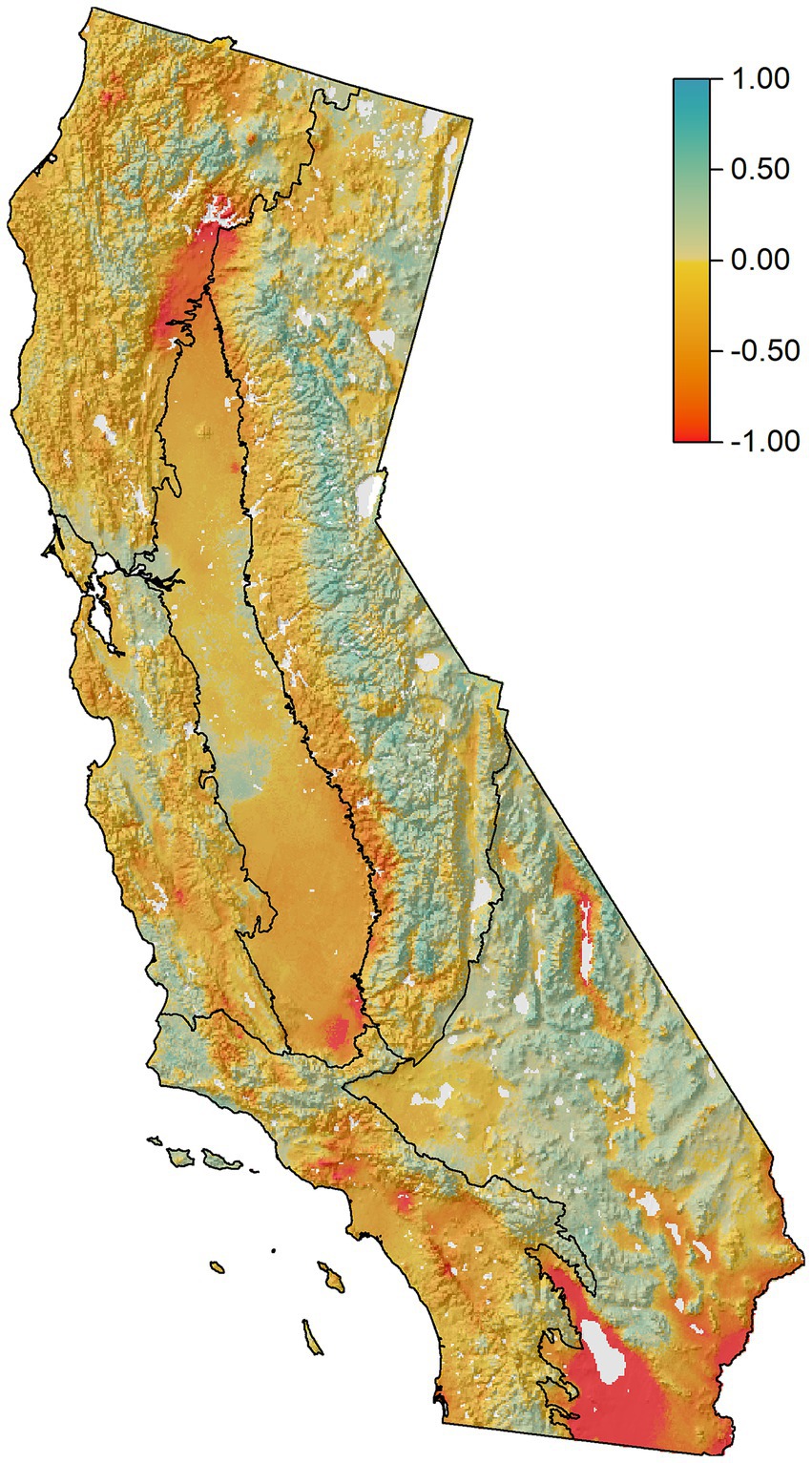
Figure 3. Final future resource stability (FRS) map. This results from averaging the FRS scores from the six individual ecosystem resource models (see Figure 4). Dark red colors indicate low resource stability (high vulnerability) to climate change across all six resources. Dark blue colors indicate consistently high stability and low vulnerability across resources.

FIGURE 4

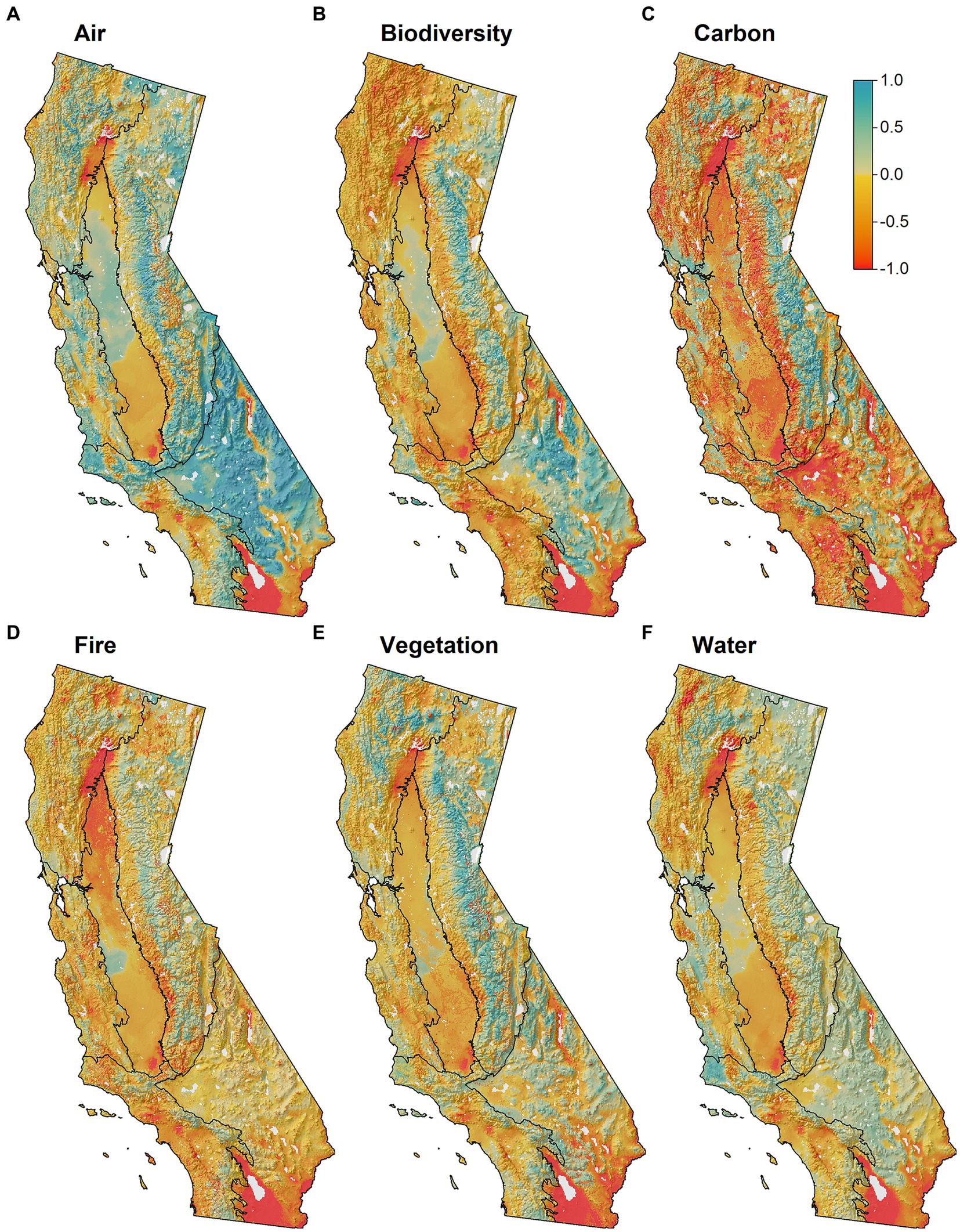
Figure 4. Future resource stability (FRS) scores across the six ecosystem resources for the state of California (1 km resolution). Color ramp is the same as in Figure 3 – red colors indicate low stability and high vulnerability to climate change, while blue colors indicate high stability and low vulnerability. Logic models are provided for each of the resource (A) Air quality, Supplementary Figure S6; (B) Biodiversity conservation, Supplementary Figure S4; (C) Carbon sequestration, Supplementary Figure S5; (D) Fire dynamics, Supplementary Figure S3; (E) Vegetation resilience, Supplementary Figure S2; (F) Water security, Supplementary Figure S7).

FIGURE 5

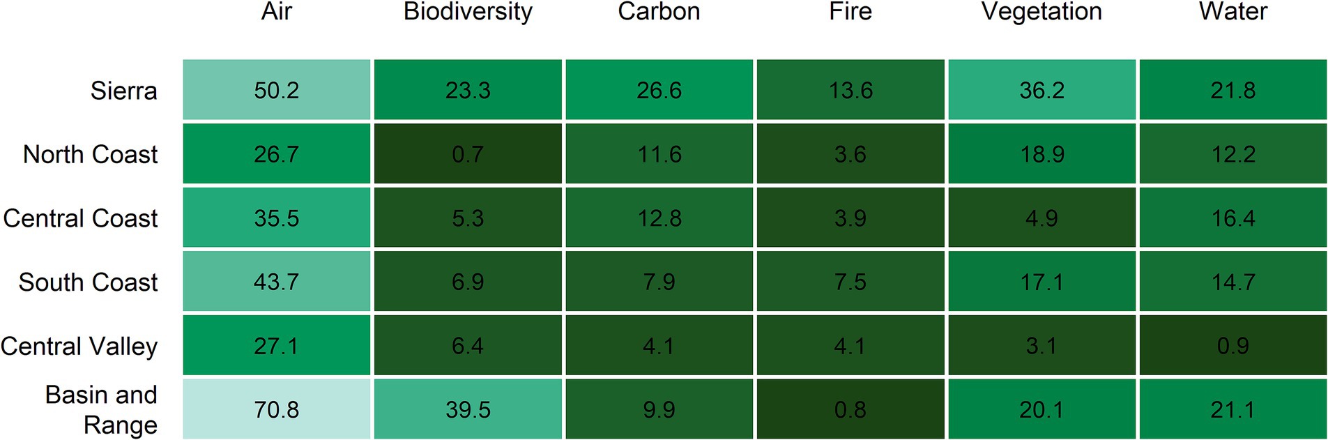
Figure 5. Percentage area of each ecoregion exhibiting high future resource stability (FRS score > 0.25) for each of the six ecosystem resources. Darker colors indicate a lower proportion of the ecoregion exhibited high FCS scores, while lighter colors indicated a higher incidence of stability.

Low stability scores in some areas resulted from poor climate analog matches overall (Supplementary Figure S9). This occurred primarily in the lower elevation portions of the South Coast and Central Coast (including the San Francisco Peninsula), southern Central Valley, southern Basin and Range, and eastern edge of the North Coast (Figures 3, 4; Supplementary Figure S9). As a reminder, each logic model included the Analog Similarity Scores (Supplementary Figure S1), which indicated how closely the climate at the analog locations matched the future climate of the focal cell. This prevented misinterpretations where the model identified high stability for a resource but where analog locations were not representative of the future climate (e.g., poor climate match; see section: Assumptions and limitations). Poor climate matches could also be indicative of non-analog future climate conditions at these locations.

In the Sierras, a clear gradient was observed from high resource stability at the mid- to upper elevations to lower stability at lower elevations and in patches on the drier eastside of the Sierras to the north (Figures 3, 4). A distinct area of high resource stability was present within this mid-to upper-elevation band in the Sierras (Figures 3, 4). Similarly, areas of higher elevation in the North Coast ecoregion exhibited consistently high stability apart from Biodiversity Conservation, which had low stability throughout the ecoregion.

The Basin and Range ecoregion was characterized by a high level of FRS for most ecosystem resources. This region is largely covered by desert ecosystems that are dominated by sparsely vegetated shrublands with some hardwood and conifer vegetation at the highest elevations (Figure 1; Bailey, 1995). The high FRS is likely a function of the temperature and drought-adapted nature of the existing ecosystems and due to the region’s low productivity, which limits the amplitude of climate change responses compared with other more mesic ecoregions, such as the North Coast.

We further explored the Vegetation Resilience response to investigate conifer vegetation (in)stability throughout the state (Figure 6). The areas of highest conifer stability occurred within the North Coast along the coastal ecoregion and at higher elevations, and within the Sierra at higher elevations (Figure 6A). Conifer instability was also identified across other portions of the State and followed steep gradients particularly in the Sierra foothills, and low elevations in the North Coast ecoregion (Figure 6B). Within these areas, transitions were largely from conifer to conifer-hardwood or hardwood types. Conifer transitions directly to shrubland occurred in the drier northeast portion of the state in the Modoc and South Cascades ecoregions (Figure 6C). Overall, 31.2% of conifer forests exhibited some level of instability within the BpS conifer footprint (>50% of analogs in non-conifer types), while 18.2% exhibited high instability (>75% of analogs in non-conifer types).

FIGURE 6

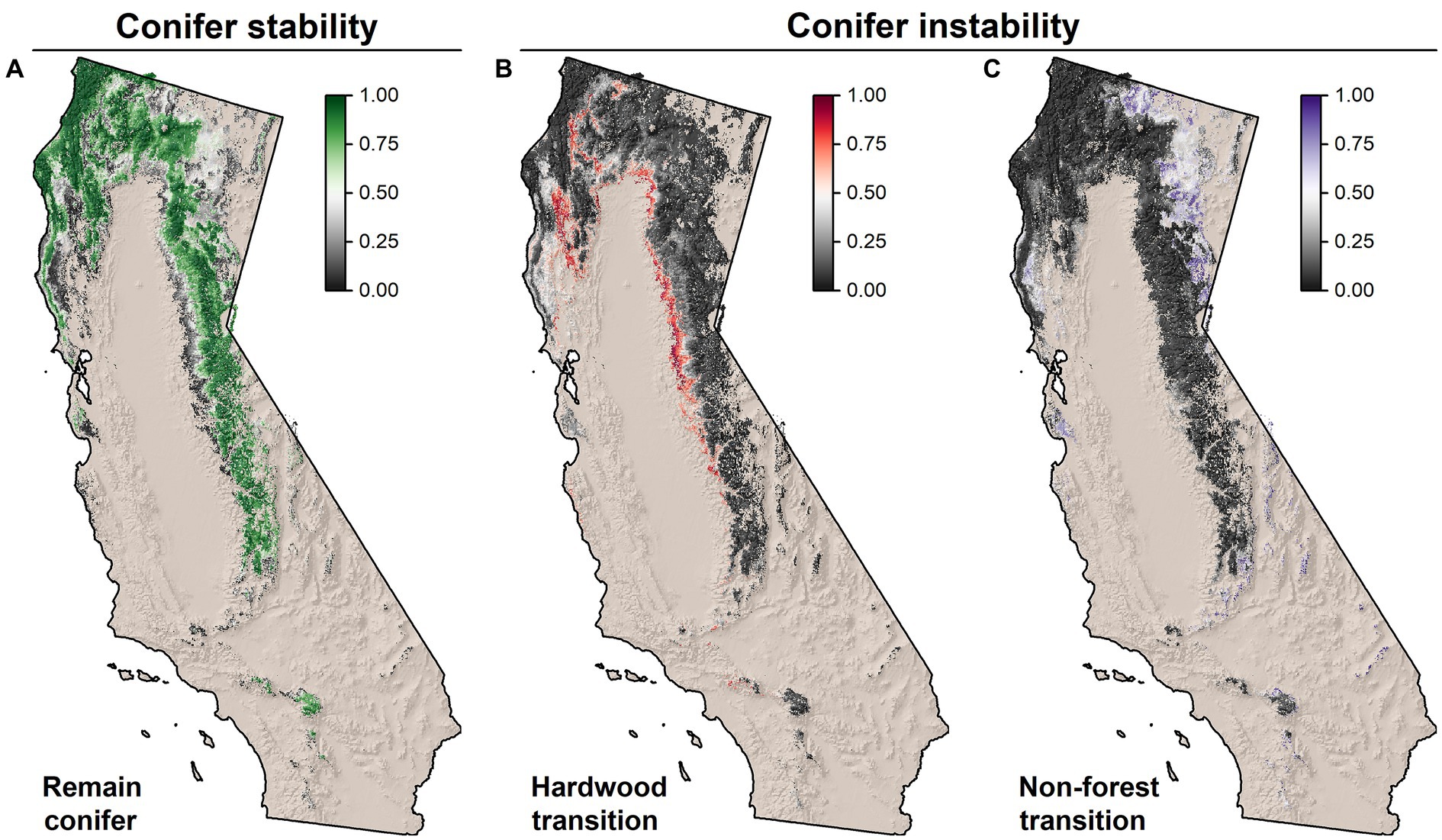
Figure 6. Climate analog modeling results depicting conifer stability and instability throughout its range in California. Stability and instability were measured as the proportion of the 900 analog locations that were (A) conifer types (i.e., stability), (B) hardwood or hardwood-conifer types, and (C) shrubland, grassland, or sparsely vegetated types. The distribution of conifer vegetation was based on LANDFIRE Biophysical Setting GROUPVEG. Dark black areas indicated no analogs matched the given vegetation type depicted in the panel, light gray areas indicate around half of the analogs were of the associated vegetation type, and brightly colored areas indicate nearly all analogs were of the vegetation type.

Random forest models were predictive of climatic conditions associated with conifer conversions to hardwood forest types (Supplementary Figure S10). Predicted conifer instability was associated with lower elevations, warm summers, and winters with precipitation dominated by rain (as opposed to snow). We found an inflection point in the response to elevation near 2,000 m, below which conifer instability increased rapidly. This corresponded well with the findings of Hill et al. (2023) who found a high incidence (95%) of vegetation-climate mismatch for Sierran conifer forests below 2,356 m (Figure 6B).

Striking similarities were observed among the PCA and K-means analyzes (Figure 7) indicating a high level of spatial structure in FRS geographic patterns. For the PCA, the first PC axis explained 59.6% of the variability in FRS scores and all loadings were positive for this PC (Table 2; Supplementary Figure S11). This suggested a high degree of correlation among ecosystem resource scores, and patterns in the PCA outputs (Figure 7A) reinforced those observed in the FRS scores (Figure 4). PC 2 explained only 17.6% of the variation and largely differentiated Carbon Sequestration from Air Quality. This is an intuitive result given that live carbon and heavy fuel loads were positively correlated (r = 0.66 across the western US) and that relatively high carbon loads at a given focal cell would indicate low FRS (i.e., carbon loads expected to decline under climate change) while comparatively high fuel loads would indicate high FRS for Air Quality (i.e., fuel loads decline under climate change).

FIGURE 7

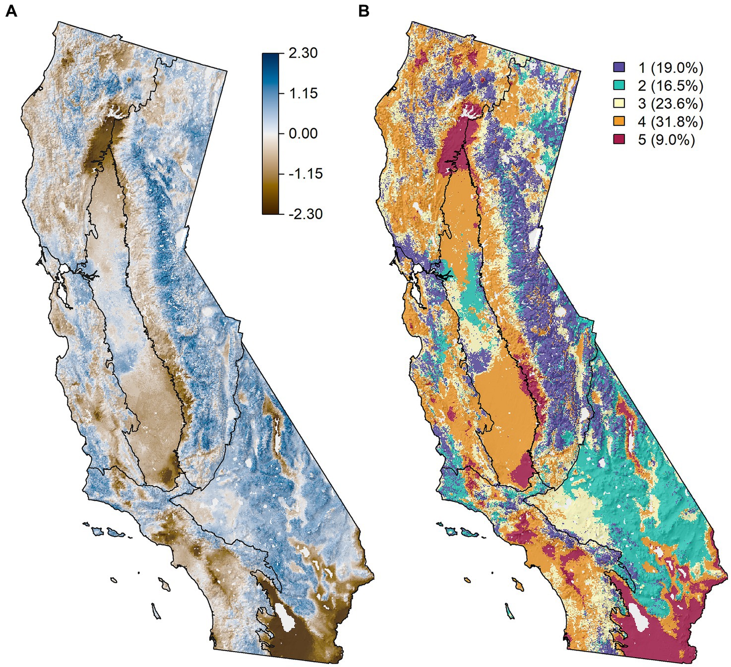
Figure 7. (A) PCA axis 1 (59.6% variance explained) from a principal components analysis on the resource stability scores across the six ecosystem resources for the state of California. Loadings were positive for all Pillars, and as such, blue areas indicate increasing stability across two or more Pillars, while brown colors indicate lower stability. (B) K-means clustering of the resource stability scores across the six ecosystem resources. K-means classes are ranked from 1, highest stability, to 5, lowest stability (see Figure 8). Percentages in the legend indicate the percentage coverage of each class across the state.

TABLE 2

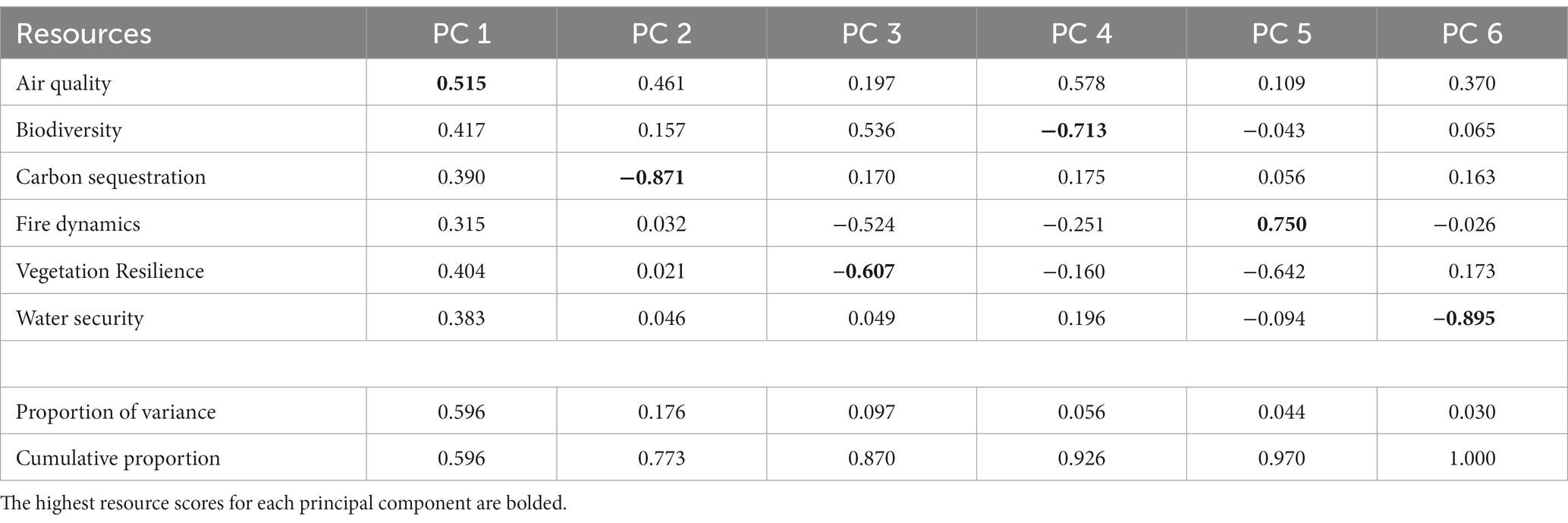
Table 2. Principal components analysis (PCA) loadings for the future resource stability scores associated with each of six ecosystem resources.

The high resource stability along the spine of the Sierra ecoregion is indicated by PC 1 as depicted in the bright blue coloration of the mapped results (Figure 7A). Focal cells along the crest of the over 600 km length of the Sierra Nevada Mountain range were associated with high Analog Similarity Scores (i.e., close matches to analog climates, Supplementary Figure S9), and resource conditions at the analog locations were similar to, or in some cases supported higher resource values than, their respective focal cell. High resource stability also existed at higher elevations in the North and Central Coast ecoregions and for the Basin and Range ecoregion. Dark brown areas observed in the southern most portions of the Basin and Range ecoregion, the foothills of the Sierra, and at the northern nexus of the Central Valley with its mountainous neighboring ecoregions indicated low stability in this region across multiple resources.

K-means analysis mirrored the findings of the PCA and identified five distinct FRS classes (Figure 7B) ranging from Class 1 (highest FRS scores overall) to Class 5 (lowest FRS scores) (Figure 8). The classification differentiated the observed PCA gradients into distinct classes that varied by the signature of the FRS scores. Class 1 (highest FRS) represented the most stable conditions for Vegetation Resilience and Carbon Sequestration, and moderate to high stability for Air Quality and Water Security, which were largely relegated to mid to high elevations in the Sierra and at higher elevations in the two coastal ecoregions. Class 2 represented the most stable conditions for Air Quality and Biodiversity Conservation, with moderate stability for Water Security, and were largely responsible for the higher stability scores observed across the Basin and Range. Conversely, Class 4 dominated the western half of the State, representing increasingly unstable conditions across all ecosystem resources, and Class 5 was limited in its distribution to a few transition areas around the Central Valley and the southern most part of the Basin and Range.

FIGURE 8

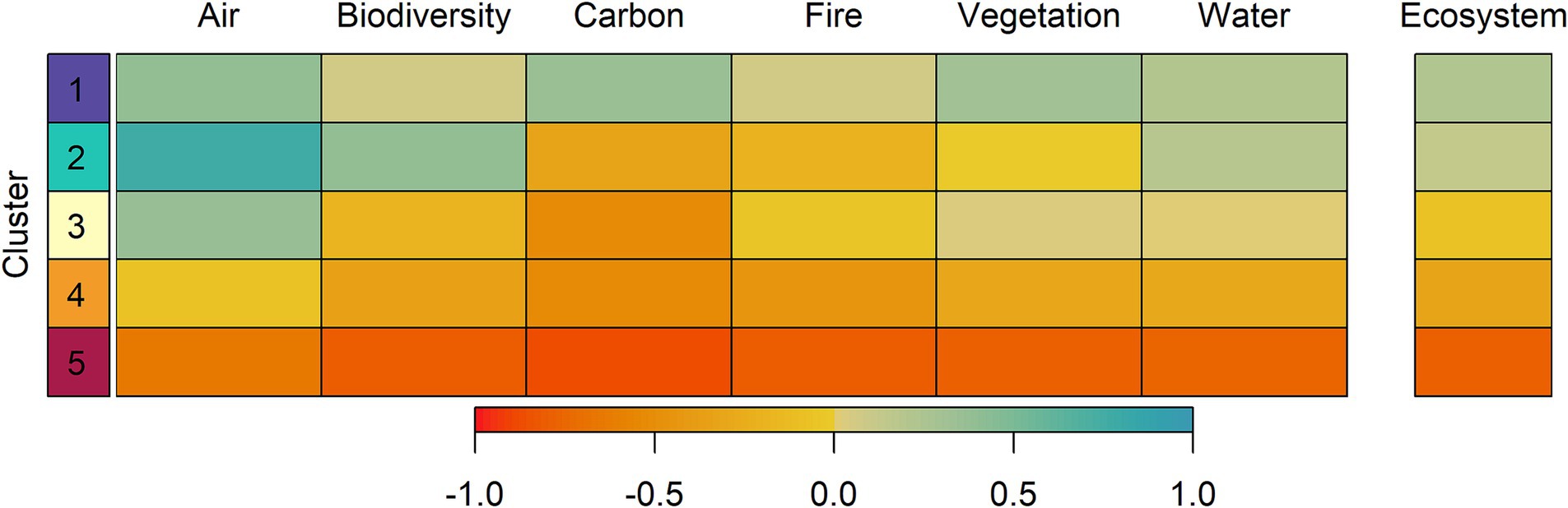
Figure 8. Average future resource stability (FRS) score for each of seven K-means clusters across the six ecosystem resources and for the final Ecosystem FRS (e.g., average of the six scores).

Question 2. What are the biophysical factors driving patterns of future resource stability across ecosystem resources?

The five FRS classes were each associated with distinct biophysical environments based on predominant temperature and precipitation regimes (Figures 9, 10). Mean warmest month temperature was the main determinant of FRS class, followed by elevation (a driver of temperature) and, to a lesser degree, mean coldest month temperature and vegetation type (Figures 9, 10). In contrast, precipitation and moisture did not emerge as factors directly associated with patterns in future resource stability. Class 1 (highest overall stability, more mountainous areas) was most strongly associated with cooler summer temperatures (<28.1°C), higher elevations (>1,114 m), and cold forest types. Class 2 (moderate overall stability, primarily Great Basin and desert areas) was primarily associated with warmer summer temperatures, moderate elevations, and cooler winter temperatures (<11.6°C). Class 3 (variable stability across resources, limited distribution, primarily located along the interface between stable and unstable areas) was not well predicted by the ctree model and was distributed across the terminal nodes, but in general was associated with cooler summer temperatures at mid-elevations. Class 4 (moderately unstable future climate across all resources, widespread across the western half of California) was associated with lower elevations and warmer summer and winter temperatures. Class 5 occurred largely at the lowest elevations areas with the warmest summer temperatures, corresponding to areas without the mitigating influences of the ocean or mountains, which may explain the incidence of no-analog conditions identified for this class (Figures 8, 9; Supplementary Figure S9).

FIGURE 9

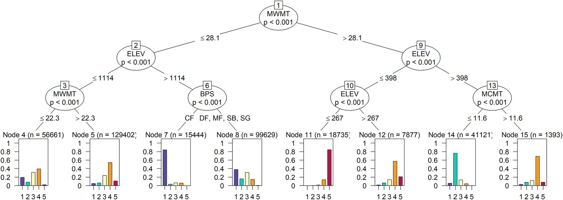
Figure 9. Conditional classification tree dendrogram depicting biophysical characteristics of each of the five K-means clusters. The color of each leaf matches the cluster membership from Figure 7B. Units are: elevation (ELEV), meters; mean coldest month temperature (MCMT), degrees C; mean warmest month temperature (MWMT), degrees C; vegetation type (BPS; CF, cold forest; DF, dry forest; MF, moist forest; SG, shrubland/grassland; SB, sparse/barren [see Parks et al. (2018)]. The cluster identifier is ordered from 1 (most stable) to 5 (least stable) (Figure 8).

FIGURE 10

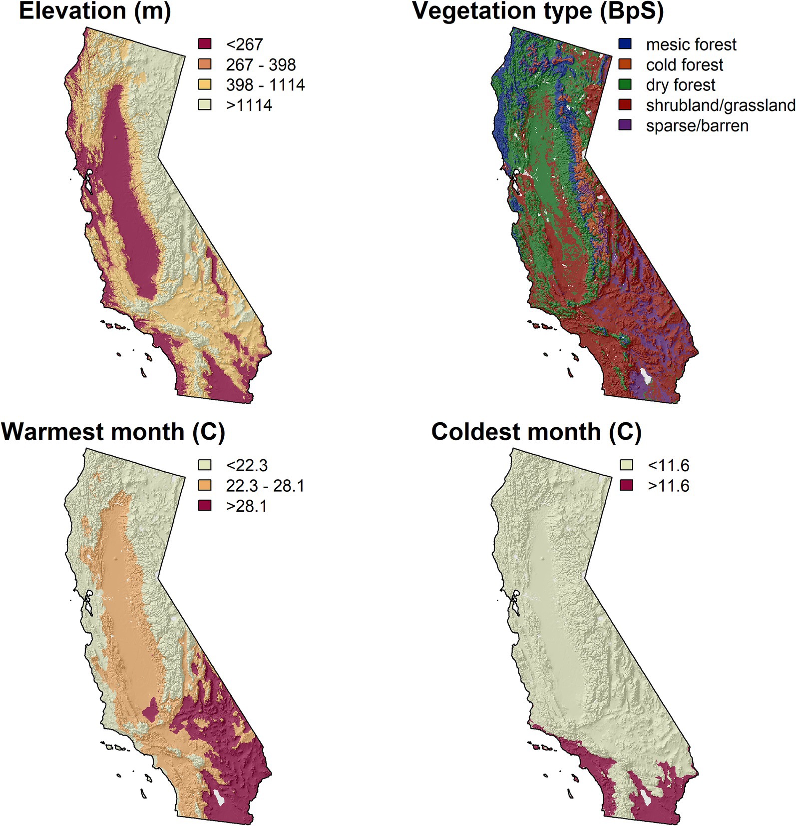
Figure 10. Maps depicting the cutoff values identified in the classification tree analysis used to explain biophysical characteristics for the K-means clusters across the six pillars. See Figure 7B for the map of the K-means clusters and Figure 9 for the classification tree diagram. Vegetation classes were based on a classification of BpS types from Parks et al. (2018).

Question 3. How do inferences about resource stability differ using climate velocity (e.g., distance to climate analogs) versus a functional assessment (e.g., FRS scores).

We found that climate velocity alone had virtually no relationship with future resource stability. Climate analogs further from their focal cell were not consistently associated with higher or lower FRS scores, regardless of the GCM (Table 3). This evidence suggests that climate velocity inferences are not generalizable to future resource stability.

TABLE 3

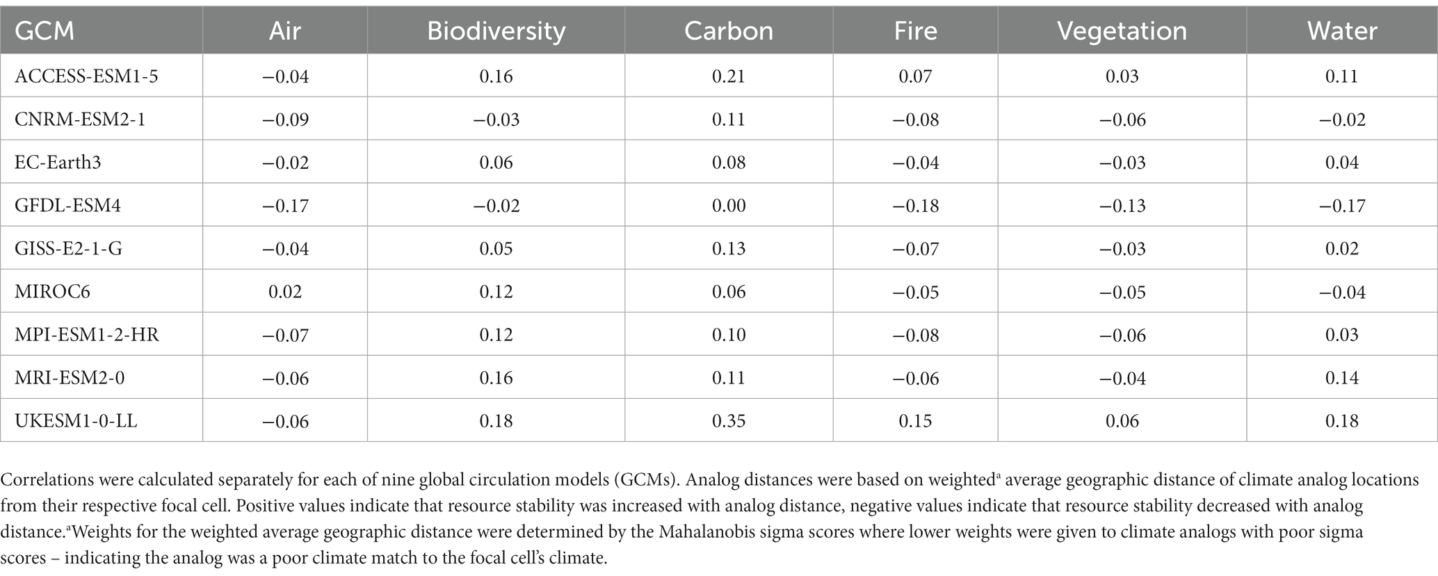
Table 3. Pearson correlation between the analog distances from the focal cell and derived measures of future resource stability for each of six ecosystem resources (Pillars).

Discussion

Climate will continue to be a major catalyst of change across ecosystems creating high uncertainty for allocating strategic management investments (Stein et al., 2014; Grafton et al., 2019; Schuurman et al., 2020; Hessburg et al., 2021). Climate-informed management frameworks have recently gained attention by providing alternative management pathways to consider under future projected climate impacts (Aplet and Cole, 2010; Peterson St-Laurent et al., 2021). However, few of these frameworks provide the necessary specificity to diagnose future conditions across large landscapes at high-resolution, provide resource-specific estimates of climatic stability, or offer a mechanism for quantifying potential future vulnerabilities. The method developed here integrates climate analog modeling with fuzzy logic evaluations to compare current ecosystem conditions with likely future trajectories under climate change. By evaluating a total of nine GCM models, our methods accounted for the high inter-model variability in future predicted climate conditions towards developing a robust estimate of ecosystem vulnerabilities to future climate. Incorporating fuzzy logic modeling into the assessment allowed us to quantify the direction and magnitude of change anticipated under future climates and relate that to a quantitative representation of future resource stability (FRS) for each of six ecosystem resources.

Using these methods, we found:

1. High spatial cross-correlation existed among the six FRS scores across California despite the highly varied data sources accompanying the resource assessments. This was in part due to a lack of adequate climate analogs across portions of the State.

2. Approximately 31% of conifer-capable forestland showed some evidence of instability (>50% of analog locations were non-conifer types). Transitions to hardwood types were indicated in the Sierran foothills and low elevations in the North Coast; transitions directly to non-forest types were identified in the southern Cascades and Modoc regions.

3. FRS spatial patterns were highly variable within and among ecoregions and responded to elevational and biophysical gradients.

4. High FRS was identified within the Sierra Nevada Mountains, at high elevations within the coastal ecoregions, and within the Basin and Range region.

5. High FRS scores were most prominent at higher elevation (>1,114-m) or at mid-elevations with warmer summers and cooler winters. Areas most vulnerable to ensuing climate change occurred at lower elevations (<398 m) and/or in warmer winter and summer environments.

These findings support previous studies showing the vulnerability of low-elevation conifer forests to current and future climatic conditions. Hill et al. (2023) found 20% of Sierra Nevada conifer forest currently inhabit areas outside their early 20th century climate envelopes, suggesting that these areas of vegetation-climate mismatch portend future conversions to non-conifer types. The most vulnerable populations in their study were found below 2,356-m elevation. Our results corroborate these findings in the Sierra and identified additional areas of conifer instability elsewhere in the State with high concentrations of climate-vulnerable conifer forests in the North Coast region in the Klamath and Trinity River drainages. Random forest analysis provided further verification, with models showing a stark increase in the likelihood of conifer to hardwood transitions at elevations <2,000-m (Supplementary Figure S10). This elevation approximates the persistent snowline for the Sierra (2250–2,500-m, Shulgina et al., 2023), which shortens the period of drought stress in conifer trees, and fuels tree growth during periods of limited rainfall (Casirati et al., 2023), among other benefits (Stevens and Latimer, 2015). Furthermore, elevation was an important predictor of FRS classes with higher elevations supporting high FRS (Class 1), while low elevations supported low FRS (Classes 4, 5). Cold forests at upper elevations exhibited high FRS, suggesting the important role these forest types play in providing a suite of stable ecosystem resources under climate change.

Thorne et al. (2017) provide an alternative assessment of potential climate change impacts on vegetation types across California. Vegetation vulnerability to climate change in their study was inferred where future climate conditions were in the extremes of the climate envelope for the vegetation type. Under warming and drying conditions, the authors found 19–24% of California’s vegetation will experience climatic stress by the mid-21^st century. Spatial patterns were similar to the Vegetation Resilience results presented here with a few exceptions, including in the Central Coast ecoregion where our finding of low stability contrasted with Thorne’s finding of generally low climatic stress.

Similar approaches have been used to infer stability of other ecosystem resources outside of vegetation. For example, Coffield et al. (2021) used a multi-model approach, including climate analog modeling, to quantify potential carbon losses and gains by 2100 across California. The authors found carbon losses of 6–33% by end-of-century and identified similar spatial patterns as our FRS representation. These estimates were validated by the authors using alternative niche-based and machine learning approaches to predict future carbon levels under climate change. Using our methodology, we found a corresponding potential carbon loss of 14.5% by mid-century. We note that Coffield et al. (2021) used a single climate analog for each focal cell and assessed carbon trajectories separately for a set of GCM scenarios, whereas we assessed the average carbon loss over a distribution of 900 analogs across 9 GCMs. Both approaches identified stable carbon at high elevation areas, particularly in the Sierra and North Coast, compared with low lying areas in the Sierra foothills, coastal sections, and arid regions where moderate to substantial carbon declines are anticipated.

Previous climate analog studies have used the geographic distance to climate analog locations as a measure of the potential challenges for organisms to track the velocity of anticipated climate change to stay within its climatic tolerances (Burrows et al., 2014). Further distances would indicate a higher velocity is required to remain within their climatic niche. These assessments are often not organism- or resource-specific and they often serve as a general assessment of potential climatic impediments. We found little to no relationship between the geographic distance to analog locations and their FRS scores across the ecosystem resources. Similarly, Coffield et al. (2021) found that their climate analog approach was insensitive to the search window size used to identify climate analogs. This suggests caution when interpreting climate velocity outputs. While analog locations further in geographic space may imply dispersal or other physical barriers for organisms, it does not necessarily indicate a direct relationship to functional ecosystem resource responses under climate change (Yegorova et al., 2021).

Climate-informed decision-making

Given the uncertainties associated with future climate impacts on ecosystem function, managers require science-based methods to strategically allocate project areas on the landscape where treatments can improve and sustain ecosystem functions into the future and where they cannot (Millar et al., 2007; Chapin et al., 2010; Millar and Stephenson, 2015). Landscape assessments reliant on current conditions alone without integrating evaluations of future potential climate may lead to lower management efficacy (i.e., return on investment; Williams, 2022). The methods introduced here incorporate future climate change modeling into landscape-level evaluations of specific ecosystem resources. The climate analog approach, combined with fuzzy logic modeling, allowed for a consistent methodology to quantitatively assess potential resource stability across large landscapes. We found that stability was similar across ecosystem resources and was largely driven by predictable elevational and biophysical gradients. As such, areas with low FRS may require a different management approach to prepare ecosystems for changing environmental conditions or assist in their transition to types that are more suited for the future prevailing climate (Schuurman et al., 2020). Such analyzes can also help identify the natural capacity for specific landscapes to supply and maintain ecosystem services over time.

The methods introduced here can contribute to the integration of climate change vulnerability assessments into climate-informed management frameworks [e.g., resist-accept-direct (RAD, Schuurman et al., 2020); resist-resilience-transformation (RRT, Peterson St-Laurent et al., 2021); resistance-resilience-response (Millar et al., 2007)]. Collectively, these approaches reflect nature-based solutions aimed at working within the parameters of natural systems in terms of the potential for sustaining existing states and setting realistic management expectations given anticipated climate impacts on resource conditions and functions (Seddon et al., 2021). These frameworks acknowledge that ecosystems are non-stationary, particularly as climate change continues to challenge the capacity to maintain characteristic processes and functions. While this represents a leap forward in terms of managing for change rather than resistance to change (Morecroft et al., 2019), there remains a need to provide a standardized and adaptable methodology to generate a quantitative, spatially explicit representation of potential stability for ecosystem resources targeted by management across large landscapes.

For example, given the large scale and scope of ecosystem changes in forestlands across the western US, planning and management agencies are directed to increase the pace and scale of management to meet these challenges (North et al., 2012; Urgenson et al., 2017; Miller et al., 2020). Strategic planning is required to best allocate restoration treatments across the region to achieve multiple objectives including risk reduction to communities, improving biodiversity, securing freshwater sources, mitigating the negative effects of wildfires, among many others. Povak et al. (This issue) introduce the PROMOTe model that allows for the joint assessment of current conditions and future resource stability measures into a single decision support modeling framework. In their article, the authors leveraged a landscape simulation model (LANDIS-II) to model future conditions to mid-21st century under natural disturbances and climate change. Model outputs were used to identify areas of stable and unstable carbon across a million-hectare landscape in the central Sierras and, along with a current conditions assessment, provided quantitative support for a set of four management strategies (Monitor, Adapt, Protect, and Transform) to help achieve carbon objectives. These methods are adaptable to the full spectrum of social-ecological resources (Manley et al., This issue).

LANDIS-II has been widely adopted given its ability to depict the evolution of modeled in situ dynamics over time (Scheller et al., 2007; Manley et al., 2023; Salter et al. 2023), and their implications for climate-induced change in resource conditions and functions. However, these models require expert knowledge to parameterize a given landscape, and processing times can be limiting for large regions at high resolution (Furniss et al., 2022). Climate analog modeling offers an alternative approach that captures observed ex situ dynamics that evolved under a given climatic and biophysical setting, and disturbance regime. Therefore, despite their fundamental differences, both approaches are aimed at quantifying the ecological implications of climate change and their downstream effects on the sustainability of social-ecological resources. Accordingly, where expertise or time prevent the application of a landscape simulation model, climate analog models appear to provide a robust estimation of FRS across the social-ecological resource gradient and can be included in climate-informed strategic landscape planning models.

Assumptions and limitations

Climate change impacts alone have a lag time, and low FRS does not necessarily indicate immediate loss of ecosystem function (Coop et al., 2020; Hoecker et al., 2023). Transitions to new states will likely be initiated by wildfire or other natural disturbances, particularly in climate change susceptible locations (Donato et al., 2016; Parks et al., 2019). Parks et al. (2019) found that ~36% of forestland across the intermountain West will be climatically unsuitable for supporting forest vegetation (i.e., trailing edge forests), and 18% of these forests are at risk of fire-caused conversion to non-forest. We similarly found evidence for potential instability in 31% of conifer-capable forestland in California, suggesting that climate may be an impediment to sustaining current levels of conifer forests across portions of the state. The increasing extent and severity of wildfires across much of the western US will likely leave many climate-sensitive areas vulnerable to conversions in the coming decades (Dennison et al., 2014; Parks and Abatzoglou, 2020; Hoecker et al., 2023).

An important component of the fuzzy logic modeling was the inclusion of the Analog Stability Score for each resource assessment, which contributed to high cross-correlation among FRS scores. Areas where climate analogs were poor matches to their focal cell received a lower score regardless of their resource condition. Therefore, focal cells with only a few close climate matches exhibited low FRS in our analysis. The choice of including the top 100 analogs per GCM could have affected the FRS results by potentially overemphasizing the influence of poor analogs in the logic calculations particularly in no-analog (or few-analog) locations. However, analog scores were derived using weights where more climatically dissimilar neighbors were weighted lower than closer neighbors. Furthermore, tests conducted using 10–100 neighbors for Vegetation Resilience FRS scores showed the number of neighbors included in the analysis had a minimal effect on FRS scores overall. Specifically, the area with FRS scores >0.25 decreased only slightly from 29.9 to 24.2% when the number of nearest neighbors included in the analysis increased from 10 to 100 per GCM.

Vegetation Resilience was characterized by LANDFIRE BpS data, which represents potential vegetation conditions under active disturbance regimes for a given biophysical setting (Rollins, 2009). Caution is warranted in comparing these results to other studies based on existing vegetation (e.g., Donato et al., 2016; Steel et al., 2022; Hill et al., 2023; Hoecker et al., 2023). Our climate analog models are not acutely predictive of future conditions or descriptive of past conditions. Analogs represent ecosystem conditions in relative equilibrium with their climate (Parks et al., 2018). The models therefore identified the climatic sensitivity of ecosystem properties to the dominant climate regime.

Analog-derived conversions from conifer to shrubland/grassland in parts of California (Figure 6) also indicated conversions from fire regimes associated with forested vegetation to those associated with these other cover types. For example, some shrublands are adapted to frequent fires while others, like chapparal, experience fires at less frequent (40–60 years) intervals (Keeley and Fotheringham, 2001). Most shrubland and grasslands burn at high severity. Therefore, changes in fire regime reflect not just climate influences but also reflect changes in predominant lifeform (Parks et al., 2018).

The desert-dominated ecoregion in our study (Basin and Range) exhibited moderate to high stability (Class 2) over much of the area. Given the existing climatic limitations on resource provisions in this area, this result should not be interpreted as an indication that resources are projected to improve by mid-century. Current resource levels in this area were demonstrably low for the State and FRS results suggest they will remain low or improve slightly. Therefore, FRS outputs should be interpreted by resource planners with reference to current inventory levels (Povak et al., This issue).

Air Quality and Carbon Sequestration assessments both utilized datasets representing a snapshot in time (2016 and 2010, respectively), which is contrary to the BpS data used for Vegetation Resilience and Fire Dynamics FRS scores. For these two resources, data were less readily available to evaluate fundamental potential. As mentioned, the BpS data provide data on the potential conditions given the prevailing biophysical environment and a disturbance regime similar to that of the pre-European settlement period. For much of California, fires were generally more frequent and less severe than today and as a result, fire as a frequent disturbance likely trumped the influence of productivity gradients on accumulating live and dead carbon (Johnston et al., 2016; Prichard et al., 2021). Therefore, the potential Air Quality and Carbon Sequestration capacity of a given site may be lower than current under an active disturbance regime (Harris et al., 2019). Given that much of the western US is currently under a fire deficit (Parks et al., 2015; Haugo et al., 2019), it is likely that carbon and large fuels currently exceed their pre-European settlement era levels across much of the western US. Across 900 analog locations, these data may be more informative of site potential to accumulate large fuels and aboveground live carbon. However, caution should be taken in the interpretation of these results given they represent existing conditions, which have been subjected to natural and human-caused disturbances. The similarity in our Carbon Sequestration results to those of Coffield et al. (2021) provides some validation for the robustness of the results from these methods.

Conclusion

Taken together, California is likely to experience a high degree of climate-driven changes in the coming decades. These will be pronounced where disturbances from fire, insects, and drought provide the catalyst for change in climate-vulnerable environments (Parks et al., 2019; Coop et al., 2020; Davis et al., 2023). Recovery to previous conditions following disturbances is less assured where climate is predicted to be an impediment to resource conditions moving forward (Parks et al., 2015; Thorne et al., 2017; Stewart et al., 2021). Future resource stability was highly variable across the State, but distinct elevational and climatic gradients were predictive of FRS scores and indicated that low elevation areas are most vulnerable to potential future climate conditions. Methods presented here extend the utility of previous climate analog modeling by including fuzzy logic evaluations of potential climate impacts across a range of ecosystem resources. Model outputs provide land managers with a high-resolution (1 km) and spatially resolved means to characterize potential climate impacts to the future sustainability of resource conditions. Such outputs can be directly integrated into decision support models that aid in strategic planning efforts to guide treatment placement and/or identify tactical options for directing transformative changes on the landscape where climate is likely unsuitable for sustaining conditions over time.

Data availability statement

The original contributions presented in the study are included in the article/Supplementary materials, further inquiries can be directed to the corresponding author.

Author contributions

NP: Conceptualization, Data curation, Formal analysis, Investigation, Methodology, Project administration, Software, Validation, Visualization, Writing – original draft. PM: Funding acquisition, Project administration, Supervision, Methodology, Writing – review & editing.

Funding

The author(s) declare financial support was received for the research, authorship, and/or publication of this article. Project partially funded by the Infrastructure Investment and Jobs Act of 2021, also known as the Bipartisan Infrastructure Law (BIL); and the Inflation Reduction Act (IRA) of 2022, and CalFire grant 8CA06227.

Acknowledgments

The authors would like to thank Sean Parks for early discussions on the climate analog modeling and supplying some initial code. We thank Kathy Zeller and Kira Hefty for initial conversations about climate analog modeling and their potential applications. We thank Paul Hessburg for continued discussions on modeling approaches and implications of our results. Finally, we thank Colin Mahony for helpful advice on calculating the Mahalanobis distance.

Conflict of interest

The authors declare that the research was conducted in the absence of any commercial or financial relationships that could be construed as a potential conflict of interest.

Publisher’s note

All claims expressed in this article are solely those of the authors and do not necessarily represent those of their affiliated organizations, or those of the publisher, the editors and the reviewers. Any product that may be evaluated in this article, or claim that may be made by its manufacturer, is not guaranteed or endorsed by the publisher.

Supplementary material

The Supplementary material for this article can be found online at: https://www.frontiersin.org/articles/10.3389/ffgc.2023.1286980/full#supplementary-material

References

Aplet, G. H., and Cole, D. N. (2010). “The trouble with naturalness: rethinking park and wilderness goals” in BeNaturalness: Rethinking Park Wilderness Stewardship in an Era of Rapid Change. eds. L. Yung and D. N. Cole (Washington, DC: Island Press)

Google Scholar

Bailey, R. G. (1995). Description of the ecoregions of the United States. USDA Forest Service, Washington, DC.

Google Scholar

Brice, E. M., Miller, B. A., Zhang, H., Goldstein, K., Zimmer, S. N., Grosklos, G. J., et al. (2020). Impacts of climate change on multiple use management of Bureau of Land Management land in the intermountain west, USA. Ecosphere 11:e03286. doi: 10.1002/ecs2.3286

CrossRef Full Text | Google Scholar

Burrows, M. T., Schoeman, D. S., Richardson, A. J., Molinos, J. G., Hoffmann, A., Buckley, L. B., et al. (2014). Geographical limits to species-range shifts are suggested by climate velocity. Nature 507, 492–495. doi: 10.1038/nature12976

PubMed Abstract | CrossRef Full Text | Google Scholar

Caetano, G. H. D. O., Chapple, D. G., Grenyer, R., Raz, T., Rosenblatt, J., Tingley, R., et al. (2022). Automated assessment reveals that the extinction risk of reptiles is widely underestimated across space and phylogeny. PLoS Biol. 20:e3001544. doi: 10.1371/journal.pbio.3001544

PubMed Abstract | CrossRef Full Text | Google Scholar

California Wildfire and Forest Resilience Task Force . (2022). Calfornia's Strategic Plan for Expanding the Use cf Beneficial Fire. Available at: https://wildfiretaskforce.org/wp-content/uploads/2023/04/californiawildfireandforestresilienceactionplan.pdf

Google Scholar

Casirati, S., Conklin, M. H., and Safeeq, M. (2023). Influence of snowpack on forest water stress in the Sierra Nevada. Front. For. Glob. 6:1181819. doi: 10.3389/ffgc.2023.1181819

CrossRef Full Text | Google Scholar

Chapin, F. S., Carpenter, S. R., Kofinas, G. P., Folke, C., Abel, N., Clark, W. C., et al. (2010). Ecosystem stewardship: sustainability strategies for a rapidly changing planet. Trends Ecol. Evol. 25, 241–249. doi: 10.1016/j.tree.2009.10.008

PubMed Abstract | CrossRef Full Text | Google Scholar

Coffield, S. R., Hemes, K. S., Koven, C. D., Goulden, M. L., and Randerson, J. T. (2021). Climate-driven limits to future carbon storage in California's wildland ecosystems. AGU Adv. 2:e2021AV000384. doi: 10.1029/2021AV000384

CrossRef Full Text | Google Scholar

Coop, J. D., Parks, S. A., Stevens-Rumann, C. S., Crausbay, S. D., Higuera, P. E., Hurteau, M. D., et al. (2020). Wildfire-driven forest conversion in western North American landscapes. Bioscience 70, 659–673. doi: 10.1093/biosci/biaa061

PubMed Abstract | CrossRef Full Text | Google Scholar

Cui, M. (2020). Introduction to the k-means clustering algorithm based on the elbow method. Accounting, Auditing and Finance 1, 5–8. doi: 10.23977/accaf.2020.010102

CrossRef Full Text | Google Scholar

Daly, C., and Bryant, K., (2013). The PRISM climate and weather system—An introduction. Corvallis, OR: PRISM climate group, 2.

Google Scholar

Daly, C., Taylor, G. H., Gibson, W. P., Parzybok, T. W., Johnson, G. L., and Pasteris, P. A. (2000). High-quality spatial climate data sets for the United States and beyond. Transact. ASAE 43, 1957–1962. doi: 10.13031/2013.3101

PubMed Abstract | CrossRef Full Text | Google Scholar

Davis, K. T., Robles, M. D., Kemp, K. B., Higuera, P. E., Chapman, T., Metlen, K. L., et al. (2023). Reduced fire severity offers near-term buffer to climate-driven declines in conifer resilience across the western United States. Proc. Natl. Acad. Sci. 120:e2208120120. doi: 10.1073/pnas.2208120120

PubMed Abstract | CrossRef Full Text | Google Scholar

Dennison, P. E., Brewer, S. C., Arnold, J. D., and Moritz, M. A. (2014). Large wildfire trends in the western United States, 1984–2011. Geophys. Res. Lett. 41, 2928–2933. doi: 10.1002/2014GL059576

CrossRef Full Text | Google Scholar

Dobrowski, S. Z., Littlefield, C. E., Lyons, D. S., Hollenberg, C., Carroll, C., Parks, S. A., et al. (2021). Protected-area targets could be undermined by climate change-driven shifts in ecoregions and biomes. Commun. Earth Environ. 2:198. doi: 10.1038/s43247-021-00270-z

CrossRef Full Text | Google Scholar

Dobrowski, S. Z., and Parks, S. A. (2016). Climate change velocity underestimates climate change exposure in mountainous regions. Nat. Commun. 7:12349. doi: 10.1038/ncomms12349

CrossRef Full Text | Google Scholar

Dobrowski, S. Z., Thorne, J. H., Greenberg, J. A., Safford, H. D., Mynsberge, A. R., Crimmins, S. M., et al. (2011). Modeling plant ranges over 75 years of climate change in California, USA: temporal transferability and species traits. Ecol. Monogr. 81, 241–257. doi: 10.1890/10-1325.1

CrossRef Full Text | Google Scholar

Donato, D. C., Harvey, B. J., and Turner, M. G. (2016). Regeneration of montane forests 24 years after the 1988 Yellowstone fires: a fire-catalyzed shift in lower treelines? Ecosphere 7:e01410. doi: 10.1002/ecs2.1410

CrossRef Full Text | Google Scholar

Fick, S. E., and Hijmans, R. J. (2017). WorldClim 2: new 1-km spatial resolution climate surfaces for global land areas. Int. J. Climatol. 37, 4302–4315. doi: 10.1002/joc.5086

CrossRef Full Text | Google Scholar

Furniss, T. J., Hessburg, P. F., Povak, N. A., Salter, R. B., and Wigmosta, M. S. (2022). Predicting future patterns, processes, and their interactions: benchmark calibration and validation procedures for forest landscape models. Ecol. Model. 473:110099. doi: 10.1016/j.ecolmodel.2022.110099

CrossRef Full Text | Google Scholar

Gaines, W. L., Hessburg, P. F., Aplet, G. H., Henson, P., Prichard, S. J., Churchill, D. J., et al. (2022). Climate change and forest management on federal lands in the Pacific northwest, USA: managing for dynamic landscapes. For. Ecol. Manag. 504:119794. doi: 10.1016/j.foreco.2021.119794

PubMed Abstract | CrossRef Full Text | Google Scholar

Garcia, R. A., Cabeza, M., Rahbek, C., and Araújo, M. B. (2014). Multiple dimensions of climate change and their implications for biodiversity. Science 344:1247579. doi: 10.1126/science.1247579

CrossRef Full Text | Google Scholar

Grafton, R. Q., Doyen, L., Béné, C., Borgomeo, E., Brooks, K., Chu, L., et al. (2019). Realizing resilience for decision-making. Nat. Sustain. 2, 907–913. doi: 10.1038/s41893-019-0376-1

PubMed Abstract | CrossRef Full Text | Google Scholar

Hamann, A., Roberts, D. R., Barber, Q. E., Carroll, C., and Nielsen, S. E. (2015). Velocity of climate change algorithms for guiding conservation and management. Glob. Chang. Biol. 21, 997–1004. doi: 10.1111/gcb.12736

PubMed Abstract | CrossRef Full Text | Google Scholar

Harris, L. B., Scholl, A. E., Young, A. B., Estes, B. L., and Taylor, A. H. (2019). Spatial and temporal dynamics of 20th century carbon storage and emissions after wildfire in an old-growth forest landscape. For. Ecol. Manag. 449:117461. doi: 10.1016/j.foreco.2019.117461

CrossRef Full Text | Google Scholar

Haugo, R. D., Kellogg, B. S., Cansler, C. A., Kolden, C. A., Kemp, K. B., Robertson, J. C., et al. (2019). The missing fire: quantifying human exclusion of wildfire in Pacific northwest forests, USA. Ecosphere 10:e02702. doi: 10.1002/ecs2.2702

CrossRef Full Text | Google Scholar

Hessburg, P. F., Prichard, S. J., Hagmann, R. K., Povak, N. A., and Lake, F. K. (2021). Wildfire and climate change adaptation of western North American forests: a case for intentional management. Ecol. Appl. 31:e02432. doi: 10.1002/eap.2432

CrossRef Full Text | Google Scholar

Hill, A. P., Nolan, C. J., Hemes, K. S., Cambron, T. W., and Field, C. B. (2023). Low-elevation conifers in California’s Sierra Nevada are out of equilibrium with climate. PNAS Nexus 2:pgad 004. doi: 10.1093/pnasnexus/pgad004

CrossRef Full Text | Google Scholar

Hoecker, T. J., Parks, S. A., Krosby, M., and Dobrowski, S. Z. (2023). Widespread exposure to altered fire regimes under 2° C warming is projected to transform conifer forests of the Western United States. Commun. Earth Environ. 4:295. doi: 10.1038/s43247-023-00954-8

CrossRef Full Text | Google Scholar

Hogg, E. H. (1997). Temporal scaling of moisture and the forest-grassland boundary in western Canada. Agric. For. Meteorol. 84, 115–122. doi: 10.1016/S0168-1923(96)02380-5

CrossRef Full Text | Google Scholar

Hothorn, T., Hornik, K., and Zeileis, A. (2006). Unbiased recursive partitioning: a conditional inference framework. J. Comput. Graph. Stat. 15, 651–674. doi: 10.1198/106186006X133933

PubMed Abstract | CrossRef Full Text | Google Scholar

Hothorn, T., and Zeileis, A. (2015). Partykit: a modular toolkit for recursive Partytioning in R. J. Mach. Learn. Res. 16, 3905–3909.

Google Scholar

Jenkins, C. N., Pimm, S. L., and Joppa, L. N. (2013). Global patterns of terrestrial vertebrate diversity and conservation. Proc. Natl. Acad. Sci. 110, E2602–E2610. doi: 10.1073/pnas.1302251110

PubMed Abstract | CrossRef Full Text | Google Scholar

Johnston, J. D., Bailey, J. D., and Dunn, C. J. (2016). Influence of fire disturbance and biophysical heterogeneity on pre-settlement ponderosa pine and mixed conifer forests. Ecosphere 7:e01581. doi: 10.1002/ecs2.1581

CrossRef Full Text | Google Scholar

Keeley, J. E., and Fotheringham, C. J. (2001). Historic fire regime in southern California shrublands. Conserv. Biol. 15, 1536–1548. doi: 10.1046/j.1523-1739.2001.00097.x

PubMed Abstract | CrossRef Full Text | Google Scholar

LANDFIRE (2020). Biophysical Setting Layer, LANDFIRE 2.2.0, U.S. Department of the Interior, Geological Survey, and U.S. Department of Agriculture. Available at: http://www.landfire/viewer

Google Scholar

Leutner, B., Horning, N., and Schwalb-Willmann, J. (2023). RStoolbox: Tools for Remote Sensing Data Analysis. Available at: https://github.com/bleutner/RStoolbox

Google Scholar

Levesque, K., and Hamann, A. (2022). Identifying western North American tree populations vulnerable to drought under observed and projected climate change. Climate 10:114. doi: 10.3390/cli10080114

CrossRef Full Text | Google Scholar

Littlefield, C. E., McRae, B. H., Michalak, J. L., Lawler, J. J., and Carroll, C. (2017). Connecting today's climates to future climate analogs to facilitate movement of species under climate change. Conserv. Biol. 31, 1397–1408. doi: 10.1111/cobi.12938

PubMed Abstract | CrossRef Full Text | Google Scholar

Mahony, C. R., Cannon, A. J., Wang, T., and Aitken, S. N. (2017). A closer look at novel climates: new methods and insights at continental to landscape scales. Glob. Chang. Biol. 23, 3934–3955. doi: 10.1111/gcb.13645

PubMed Abstract | CrossRef Full Text | Google Scholar

Mahony, C. R., MacKenzie, W. H., and Aitken, S. N. (2018). Novel climates: trajectories of climate change beyond the boundaries of British Columbia’s forest management knowledge system. For. Ecol. Manag. 410, 35–47. doi: 10.1016/j.foreco.2017.12.036

CrossRef Full Text | Google Scholar

Mahony, C. R., Wang, T., Hamann, A., and Cannon, A. J. (2022). A global climate model ensemble for downscaled monthly climate normals over North America. Int. J. Climatol. 42, 5871–5891. doi: 10.1002/joc.7566

CrossRef Full Text | Google Scholar

Manley, P. N., Povak, N. A., and Wilson, K. N. (This issue). A working framework for socio-ecological resilience to inform climate change management strategies across landscapes. Front. For. Glob. Change

Google Scholar

Manley, P. N, Povak, N. A., Wilson, K. N., Fairweather, M. L., Griffey, V., and Long, L. L. (2023). Blueprint for resilience: the Tahoe-central sierra initiative. General technical report PSW-GTR-277. U.S. Forest Service, Pacific Southwest Research Station. Placerville, CA

Google Scholar

McCune, B., and Grace, J. B. (2002). Analysis of ecological communities. MjM Software Design, Gleneden Beach, OR.

Google Scholar

McWethy, D. B., Schoennagel, T., Higuera, P. E., Krawchuk, M., Harvey, B. J., Metcalf, E. C., et al. (2019). Rethinking resilience to wildfire. Nat. Sustain. 2, 797–804. doi: 10.1038/s41893-019-0353-8

CrossRef Full Text | Google Scholar

Millar, C. I., and Stephenson, N. L. (2015). Temperate forest health in an era of emerging mega disturbance. Science 349, 823–826. doi: 10.1126/science.aaa9933

PubMed Abstract | CrossRef Full Text | Google Scholar

Millar, C. I., Stephenson, N. L., and Stephens, S. L. (2007). Climate change and forests of the future: managing in the face of uncertainty. Ecol. Appl. 17, 2145–2151. doi: 10.1890/06-1715.1

PubMed Abstract | CrossRef Full Text | Google Scholar

Miller, R. K., Field, C. B., and Mach, K. J. (2020). Barriers and enablers for prescribed burns for wildfire management in California. Nat. Sustain. 3, 101–109. doi: 10.1038/s41893-019-0451-7

CrossRef Full Text | Google Scholar

Morecroft, M. D., Duffield, S., Harley, M., Pearce-Higgins, J. W., Stevens, N., Watts, O., et al. (2019). Measuring the success of climate change adaptation and mitigation in terrestrial ecosystems. Science 366:eaaw9256. doi: 10.1126/science.aaw9256

CrossRef Full Text | Google Scholar

North, M., Collins, B. M., and Stephens, S. (2012). Using fire to increase the scale, benefits, and future maintenance of fuels treatments. J. For. 110, 392–401. doi: 10.5849/jof.12-021

CrossRef Full Text | Google Scholar

Ottmar, R. D., Sandberg, D. V., Riccardi, C. L., and Prichard, S. J. (2007). An overview of the fuel characteristic classification system – quantifying, classifying, and creating fuelbeds for resource planning. Can. J. For. Res. 37, 2383–2393. doi: 10.1139/X07-077

CrossRef Full Text | Google Scholar

Parks, S. A., and Abatzoglou, J. T. (2020). Warmer and drier fire seasons contribute to increases in area burned at high severity in western US forests from 1985 to 2017. Geophys. Res. Lett. 47:e2020GL089858. doi: 10.1029/2020GL089858

CrossRef Full Text | Google Scholar

Parks, S. A., Dobrowski, S. Z., Shaw, J. D., and Miller, C. (2019). Living on the edge: trailing edge forests at risk of fire-facilitated conversion to non-forest. Ecosphere 10:e02651. doi: 10.1002/ecs2.2651

CrossRef Full Text | Google Scholar

Parks, S. A., Holsinger, L. M., Abatzoglou, J. T., Littlefield, C. E., and Zeller, K. A. (2023). Protected areas not likely to serve as steppingstones for species undergoing climate-induced range shifts. Glob. Chang. Biol. 29, 2681–2696. doi: 10.1111/gcb.16629

PubMed Abstract | CrossRef Full Text | Google Scholar

Parks, S. A., Holsinger, L. M., Littlefield, C. E., Dobrowski, S. Z., Zeller, K. A., Abatzoglou, J. T., et al. (2022). Efficacy of the global protected area network is threatened by disappearing climates and potential transboundary range shifts. Environ. Res. Lett. 17:054016. doi: 10.1088/1748-9326/ac6436

CrossRef Full Text | Google Scholar

Parks, S. A., Holsinger, L. M., Miller, C., and Parisien, M. A. (2018). Analog-based fire regime and vegetation shifts in mountainous regions of the western US. Ecography 41, 910–921. doi: 10.1111/ecog.03378

CrossRef Full Text | Google Scholar

Parks, S. A., Miller, C., Parisien, M. A., Holsinger, L. M., Dobrowski, S. Z., and Abatzoglou, J. (2015). Wildland fire deficit and surplus in the western United States, 1984–2012. Ecosphere 6, 1–13. doi: 10.1890/ES15-00294.1

CrossRef Full Text | Google Scholar

Peterson, D. L., McCaffrey, S. M., and Patel-Weynand, T. (Eds), (2022). ‘Wildfire smoke in the United States, a scientific assessment.’ (Springer Publishing: New York).

Google Scholar

Peterson St-Laurent, G., Oakes, L. E., Cross, M., and Hagerman, S. (2021). R–R–T (resistance–resilience–transformation) typology reveals differential conservation approaches across ecosystems and time. Commun. Biol. 4:39.

Google Scholar

Pörtner, H. O., Roberts, D. C., Poloczanska, E. S., Mintenbeck, K., Tignor, M., Alegría, A., et al., (2022). IPCC, 2022: summary for policymakers. In: Climate change 2022: Impacts, adaptation, and vulnerability: Contribution of working group II to the sixth assessment report of the intergovernmental panel on climate change. Cambridge, UK, Intergovernmental Panel on Climate Change,

Google Scholar

Povak, N. A., Manley, P. N., and Wilson, K. N. This issue. Quantitative methods for integrating climate adaptation strategies into spatial decision support models. Front. For. Glob. Change

Google Scholar

Prichard, S. J., Andreu, A., Ottmar, R. D., and Eberhardt, E., (2019). Fuel characteristic classification system (FCCS) field sampling and fuelbed development guide. US Department of Agriculture, Forest Service, Pacific Northwest Research Station. Washington, DC

Google Scholar

Prichard, S. J., Hessburg, P. F., Hagmann, R. K., Povak, N. A., Dobrowski, S. Z., Hurteau, M. D., et al. (2021). Adapting western North American forests to climate change and wildfires: 10 common questions. Ecol. Appl. 31:e02433. doi: 10.1002/eap.2433

CrossRef Full Text | Google Scholar

R Core Team (2021). R: a language and environment for statistical computing. R foundation for statistical computing, Vienna, Austria. Available at: https://www.R-project.org/

Google Scholar

Rehfeldt, G. E., Crookston, N. L., Sáenz-Romero, C., and Campbell, E. M. (2012). North American vegetation model for land-use planning in a changing climate: a solution to large classification problems. Ecol. Appl. 22, 119–141. doi: 10.1890/11-0495.1

PubMed Abstract | CrossRef Full Text | Google Scholar

Reynolds, K. M. , (2001). Fuzzy logic knowledge bases in integrated landscape assessment: examples and possibilities. US Department of Agriculture, Forest Service, Pacific Northwest Research Station. Washington, DC

Google Scholar

Reynolds, K. M., Paplanus, S., Murphy, P. J., Druzdzel, M. J., Spenser, C., and Miller, B. J. (2023). Latest features of the ecosystem management decision support system, version 8.0. Front. Environ. Sci. 11:1231818. doi: 10.3389/fenvs.2023.1231818

CrossRef Full Text | Google Scholar

Roll, U., Feldman, A., Novosolov, M., Allison, A., Bauer, A. M., Bernard, R., et al. (2017). The global distribution of tetrapods reveals a need for targeted reptile conservation. Nat. Ecol. Evol. 1, 1677–1682. doi: 10.1038/s41559-017-0332-2

PubMed Abstract | CrossRef Full Text | Google Scholar

Rollins, M. G. (2009). LANDFIRE: a nationally consistent vegetation, wildland fire, and fuel assessment. Int. J. Wildland Fire 18, 235–249. doi: 10.1071/WF08088

CrossRef Full Text | Google Scholar

Salter, R. B., Duan, Z., and Wigmosta, M. (2023). Informing climate adaptation strategies using ecological simulation models and spatial decision support tools. Front. For. Glob. Change 6:1269081.

PubMed Abstract | Google Scholar

Scheller, R. M., Domingo, J. B., Sturtevant, B. R., Williams, J. S., Rudy, A., Gustafson, E. J., et al. (2007). Design, development, and application of LANDIS-II, a spatial landscape simulation model with flexible temporal and spatial resolution. Ecol. Model. 201, 409–419. doi: 10.1016/j.ecolmodel.2006.10.009

CrossRef Full Text | Google Scholar

Schloss, C. A., Nuñez, T. A., and Lawler, J. J. (2012). Dispersal will limit ability of mammals to track climate change in the Western hemisphere. Proc. Natl. Acad. Sci. 109, 8606–8611. doi: 10.1073/pnas.1116791109

PubMed Abstract | CrossRef Full Text | Google Scholar

Schuurman, G. W., Hoffman, C. H., Cole, D. N., Lawrence, D. J., Morton, J. M., Magness, D. R., et al., (2020). Resist-accept-direct (RAD)-a framework for the 21st-century natural resource manager (no. 2020/2213). National Park Service Washington, DC.

Google Scholar

Seddon, N., Smith, A., Smith, P., Key, I., Chausson, A., Girardin, C., et al. (2021). Getting the message right on nature-based solutions to climate change. Glob. Chang. Biol. 27, 1518–1546. doi: 10.1111/gcb.15513

PubMed Abstract | CrossRef Full Text | Google Scholar

Shulgina, T., Gershunov, A., Hatchett, B. J., Guirguis, K., Subramanian, A. C., Margulis, S. A., et al. (2023). Observed and projected changes in snow accumulation and snowline in California’s snowy mountains. Clim. Dyn. 61, 4809–4824. doi: 10.1007/s00382-023-06776-w

CrossRef Full Text | Google Scholar

Spawn, S. A., Sullivan, C. C., Lark, T. J., and Gibbs, H. K. (2020). Harmonized global maps of above and belowground biomass carbon density in the year 2010. Scientific Data 7, 1–22. doi: 10.1038/s41597-020-0444-4

CrossRef Full Text | Google Scholar

Steel, Z. L., Jones, G. M., Collins, B. M., Green, R., Koltunov, A., Purcell, K. L., et al. (2022). Mega-disturbances cause rapid decline of mature conifer forest habitat in California. Ecol. Appl. 33:e2763. doi: 10.1002/eap.2763

CrossRef Full Text | Google Scholar

Stein, B. A., Glick, P., Edelson, N., and Staudt, A. (2014). Climate-smart conservation: Putting adaptation principles into practice. National Wildlife Federation. Reston, Virginia

Google Scholar

Stevens, J. T., and Latimer, A. M. (2015). Snowpack, fire, and forest disturbance: interactions affect montane invasions by non-native shrubs. Glob. Chang. Biol. 21, 2379–2393. doi: 10.1111/gcb.12824

PubMed Abstract | CrossRef Full Text | Google Scholar

Stewart, J. A., van Mantgem, P. J., Young, D. J., Shive, K. L., Preisler, H. K., Das, A. J., et al. (2021). Effects of postfire climate and seed availability on postfire conifer regeneration. Ecol. Appl. 31:e02280. doi: 10.1002/eap.2280

CrossRef Full Text | Google Scholar

Thorne, J. H., Choe, H., Boynton, R. M., Bjorkman, J., Albright, W., Nydick, K., et al. (2017). The impact of climate change uncertainty on California’s vegetation and adaptation management. Ecosphere 8:e02021. doi: 10.1002/ecs2.2021

CrossRef Full Text | Google Scholar

Triepke, F. J., Muldavin, E. H., and Wahlberg, M. M. (2019). Using climate projections to assess ecosystem vulnerability at scales relevant to managers. Ecosphere 10:e02854. doi: 10.1002/ecs2.2854

CrossRef Full Text | Google Scholar

Urgenson, L. S., Ryan, C. M., Halpern, C. B., Bakker, J. D., Belote, R. T., Franklin, J. F., et al. (2017). Visions of restoration in fire-adapted forest landscapes: lessons from the collaborative Forest landscape restoration program. Environ. Manag. 59, 338–353. doi: 10.1007/s00267-016-0791-2

PubMed Abstract | CrossRef Full Text | Google Scholar

Wang, T., Hamann, A., Spittlehouse, D., and Carroll, C. (2016). Locally downscaled and spatially customizable climate data for historical and future periods for North America. PLoS One 11:e0156720. doi: 10.1371/journal.pone.0156720

PubMed Abstract | CrossRef Full Text | Google Scholar

Williams, J. W. (2022). RAD: a paradigm, shifting. Bioscience 72, 13–15. doi: 10.1093/biosci/biab123

PubMed Abstract | CrossRef Full Text | Google Scholar

Williams, J. W., Jackson, S. T., and Kutzbach, J. E. (2007). Projected distributions of novel and disappearing climates by 2100 AD. Proc. Natl. Acad. Sci. U. S. A. 104, 5738–5742. doi: 10.1073/pnas.0606292104

PubMed Abstract | CrossRef Full Text | Google Scholar

Wright, M. N., and Ziegler, A. (2017). Ranger: a fast implementation of random forests for high dimensional data in C++ and R. J. Stat. Softw. 77, 1–17. doi: 10.18637/jss.v077.i01

CrossRef Full Text | Google Scholar

Yegorova, S., Dobrowski, S. Z., and Parks, S. A. (2021). Should we use climate analogs to predict climate impacts? A contemporary validation. UM Graduate Student Research Conference (GradCon 4). Available at: https://scholarworks.umt.edu/gsrc/2021/stem_oral/4

Google Scholar

Young-Hart, L., Stine, P., Manley, P., and Clark, C., (2023). ACCEL metric dictionary. U.S. Department of Agriculture Forest Service. Washington, DC

Google Scholar