A preliminary view of the CYGNSS soil moisture-vegetation activity linkage

1 Introduction

Soil moisture (SM) affects ecosystems’ energy balance and climate change by altering the land surface heat capacity and the latent heat transport to the atmosphere, and vegetation growth largely depends on SM availability, especially in arid and semi-arid regions of the pan-tropical. Furthermore, previous studies have shown that spatial variations in vegetation activity and SM can change the oblique pressure structure of the surface atmosphere, which can indirectly lead to convective storms (Chang and Wetzel, 1991). Accordingly, this highlights the necessity to assess the linkage between SM and vegetation activity.

Spaceborne global navigation satellite system reflectometry (GNSS-R) is an emerging remote sensing technique that exploits the capability of GNSS satellites in a bistatic radar configuration and collects the geophysical surface-reflected signals by specially designed receivers (Chew et al., 2016; Ruf et al., 2018). In recent years, several spaceborne GNSS-R missions/payloads have been successively launched, e.g., the TechDemoSat-1 (TDS-1) launched by the U.K. in 2014, the Cyclone GNSS (CYGNSS) launched by the National Aeronautics and Space Administration (NASA) in 2016, the BuFeng-1 (BF-1) A/B twin satellites launched by China in 2019, and the GNSS Occultation Sounder-Reflectometry (GNOS-R) onboard the FengYun-3E (FY-3E) satellite launched by China in 2021 (Ruf et al., 2013; Foti et al., 2015; Jing et al., 2019; Yang et al., 2022a,b). Among these missions, CYGNSS is a representative mission with publicly available data. The CYGNSS is the first Earth Venture Class fully dedicated spaceborne GNSS-R mission, and it consists of a constellation of eight micro-satellites orbiting in the same plane at an altitude of approximately 510 km and at an orbit inclination of 35° in pan-tropical areas, which results in the specular points scattering from 38°S to 38°N. Each micro-satellite carries a four-channel GNSS-R bistatic radar receiver to collect Global Positioning System (GPS) signals (Chew and Small, 2018; Chew and Small, 2020). Here, the CYGNSS data is chosen to retrieve SM due to its unique advantages of simultaneous signals, a cost-effective alternative, and high temporal resolution.

Currently, CYGNSS SM retrieval methods can be mainly categorized into two types, i.e., empirical and multi-source auxiliary data-driven methods. The empirical method takes satellite SM product or in-situ SM as reference data, establishing the conversion relationship between spaceborne GNSS-R observables and the reference SM. The multi-source auxiliary data-driven method mainly considers the signal attenuation and diffuse reflection caused by land conditions (e.g., surface roughness, vegetation) on GNSS signals, and combines CYGNSS observables with multi-source remote sensing auxiliary data through machine learning (ML) models or radiative transfer models. In addition to the land conditions, system errors also result in various uncertainties in the CYGNSS Level 1 data observables (Gleason et al., 2018; Wan et al., 2020). In particular, as shown in previous studies, CYGNSS has inherent systematic errors, such as atmospheric attenuation, GNSS transmit power errors, and antenna gain, due to its multi-transmitter and single-receiver observing structure, resulting in inaccurate SM retrieval.

Previous studies have shown a strong sensitivity between SM and vegetation, and the sensitivity varies with vegetation type and climate. Luo et al. (2021) demonstrated that in the Mongolian Plateau, vegetation phenology showed a strong seasonal variation in response to SM. Zhao et al. (2023) utilized the long-term normalized difference vegetation index (NDVI) and the Global Land Evaporation Amsterdam Version 3a (GLEAM v3a) SM, to investigate the variation of vegetation dependence on SM in China. However, the SM used in the above studies was derived from reanalysis data or land surface models, which may have some limitations in terms of accuracy (Dong et al., 2020). In addition, the link between SM and vegetation activity needs to be further quantified in the pan-tropical region, especially in water-scarce areas.

This study aims to investigate the link between the CYGNSS SM and vegetation activity in the pan-tropical region. To achieve this objective, four years of CYGNSS SM (i.e., from January 2019 to December 2022) are matched up with two key indexes of vegetation activity, i.e., NDVI and growing season start time (SOS). First, the CYGNSS SM with system error and land surface error calibration is validated by SMAP SM. Then, CYGNSS SM is matched up with 15-day NDVI data to investigate the sensitivity of SM to vegetation in the pan-tropical region. Finally, the correlation of the CYGNSS SM and the NDVI resulting SOS from 10^o N to 38^o N is evaluated. The results of this study are expected to provide data for understanding the link between SM and vegetation activity.

2 Data

2.1 CYGNSS L1 data

The CYGNSS, with the primary objective of ocean wind speed monitoring, consists of eight low-orbit micro-satellites, with high revisit times of 2.8 ~ 7 h per day. It has a global coverage of approximately from 38°N to 38°S. The minimum spatial footprint is ~3.5 km × 0.5 km for coherent scattering from smooth surfaces (Chew and Small, 2018; Chew and Small, 2020). The science community has further explored its sensitivity to SM. The CYGNSS measurements of SM are attributed to the sensitivity of its working band to the soil permittivity. Level 1 data of CYGNSS is used in this study. Only the land data are retained. The incidence angle is set to less than 65^o during the data preprocessing process. Here, data from August to December 2018 is used for model training, and data from January 2019 to December 2022 is used for applications.

2.2 SMAP data

The Level 3 36-km SMAP gridded data produced from the radiometer is used to require global SM distribution at high accuracy. Similar to the CYGNSS data, the SMAP instrument works with an L-band radar. The SMAP turns the natural thermal emission from the soil surface into SM, with the format of Equal-Area Scalable Earth Grid 2, providing global mapping of SM every 2–3 days. Here, the SM derived from SMAP is used to convert CYGNSS observables to SM, and validation. The variable of “retrieval_qual_flag” in the SMAP product is used to identify retrievals to be of recommended quality, with either 0 or 8 indicating high-quality SM retrievals (Chan et al., 2016).

2.3 NDVI data

The NDVI used here is developed from the NASA Goddard Space Flight Center (NDVI3g dataset), generated based on the publicly available NDVI dataset from the Advanced Very High Resolution Radiometer (AVHRR). The spatial resolution of the NDVI dataset is 10 km, and the temporal resolution is 15 days. The NDVI data is resampled to 36 km based on the nearest neighbor interpolation method.

3 Method

Figure 1 shows the flowchart of this study. The main steps are summarized as follows: (1) The CYGNSS SM from January 2019 to December 2022 with land surface and system errors calibration is first retrieved; (2) The CYGNSS SM is matched to NDVI with the temporal resolution of 15 days, aiming to investigate the impact of SM on vegetation; (3) the resulting SOS from NDVI is matched up with CYGNSS SM, to analyze the spring phenology response to SM.

FIGURE 1

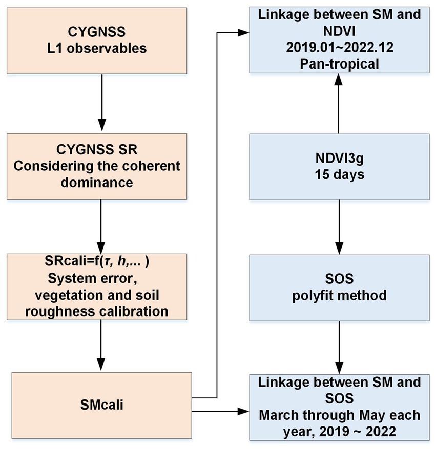
Figure 1. The flowchart of this study.

3.1 Derivation of the CYGNSS SM

Here, the reflected signal is assumed to be dominated by the coherent component. The coherent method uses the CYGNSS observable to retrieve SM based on the bistatic radar equation (Chew et al., 2016; Eroglu et al., 2019; Yan et al., 2020), as follows:

$\begin{array}{ll}{P}_{coh}^r=\frac{P_t{G}_t}{4\pi {\left(R_{ts}+R_{\mathit{sr}}\right)}^2}\frac{G_r{\lambda }^2}{4\pi }\Gamma \left({\epsilon }_S,\theta \right)& (1)\end{array}$

where P_t is the transmitted right-handed circularly polarized (RHCP) power of GNSS satellites; G_t and G_r are the gain of the transmitter antenna and the gain of the receiver antenna, respectively; R_ts and R_sr are the distance from the transmitter to the specular reflection point and the distance from the specular reflection point to the receiver, respectively; λ (m) is the wavelength of the GPS L band; Γ is the surface reflectivity (SR) without accurate calibration, hereafter named SR_raw.

As mentioned above, the CYGNSS mission has system errors. System errors play a role when constraining the output observables. Therefore, the SR_raw needs to be calibrated from system bias. Moreover, the land surface properties, i.e., vegetation and surface roughness, can also cause signal attenuation and diffuse reflections, resulting in random errors in GNSS signals. Thus, the land surface properties also need to be calibrated to get accurate soil reflectively from SR. In summary, two calibration steps are then carried out on the SR_raw, to get accurate soil reflectively. For the system error calibration, Wan et al. (2020) proposed a calibration method to eliminate the system errors of the CYGNSS level 1 data. The core concept of the method is using the theoretical Fresnel reflectivity of the calm and clean inland water bodies to calibrate the SR_raw of the land surface.

The theoretical Fresnel reflectivity of water is calculated using the following equation:

$\begin{array}{ll}{\Gamma }_w=\frac{{\left({\epsilon }_w-1\right)}^2{cos}^2\left(\theta \right)\left({\epsilon }_w-{sin}^2\left(\theta \right)\right)}{{\left({\epsilon }_{w}sin\left(90-\theta \right)+\sqrt{{\epsilon }_w-{sin}^2\left(\theta \right)}\right)}^2{\left(sin\left(\theta \right)+\sqrt{{\epsilon }_w-{sin}^2\left(\theta \right)}\right)}^2}& (2)\end{array}$

where Γ_w represents the theoretical Fresnel reflectivity of water, ε_w is the water permittivity (ε_w = 80), and θ is the incidence angle.

The SR_raw after system errors calibration, hereafter named SR_cali, is obtained by:

$\begin{array}{ll}{\Gamma }_{\mathit{cali}}={\Gamma }_{\mathit{raw}}\ast \frac{{\Gamma }_w}{{\Gamma }_{\mathit{raw}:w}}& (3)\end{array}$

For the second calibration step, we have made initial attempts to calibrate the attenuation due to vegetation and surface roughness on the CYGNSS SR by proposing a physics-based algorithm using SMAP brightness temperature (T_Bp) (Yang et al., 2022a,b).

The SR_cali can be calibrated to soil reflectivity using the following expression:

$\begin{array}{ll}{\Gamma }_{\mathit{soil}}={\Gamma }_{\mathit{cali}}\ast exp\left(-2\mathit{\tau sec\theta }-h{cos}^2\theta \right)& (4)\end{array}$

where ${\Gamma }_{\mathit{soil}}$ is the final soil reflectivity; τ is the vegetation optical depth (VOD); θ is the incidence angle; h is the surface roughness parameter.

As expressed by Yang et al., 2022a,b, the combined parameter, i.e., $exp\left(-2\mathit{\tau sec\theta }-h{cos}^2\theta \right)$ can be derived by the zeroth-order radiative transfer model. The algorithm relies on SMAP brightness temperature (T_BP) as the only parameter. The combined parameter $exp\left(-2\mathit{\tau sec\theta }-h{cos}^2\theta \right)$ can be expressed as:

$\begin{array}{ll}exp\left(-2\mathit{\tau sec\theta }-h{cos}^2\theta \right)=\frac{T_{BV}-T_{BH}}{T_{BV}{R}_{H:s}-T_{BH}{R}_{V:s}}& (5)\end{array}$

where T_BV and T_BH represent V and H polarized T_BP, respectively; $R$H_s and $R$V_s refer to the Fresnel reflection coefficient at a smooth dielectric boundary of V and H polarization, respectively, which can be expressed as the soil permittivity and the incidence angle using Fresnel equations (Choudhury et al., 1979). The readers are referred to Yang et al., 2022a,b for detailed information. Box 1 illustrates the equations and ancillary variables required by the model.

BOX 1. SR calibration steps.

The GNOS-R and CYGNSS soil reflectivity are correlated with SMAP SM using linear regression for each grid calculated from the number of points. The final CYGNSS SM can be expressed as:

$\begin{array}{ll}{\mathrm{S}\mathrm{M}}_{\mathrm{CYGNSS}}=\beta \ast {\Gamma }_{\mathit{soil}}+\alpha & (6)\end{array}$

where β and α are the slope and the intercept of the linear regression. The CYGNSS SM is finally resampled to 36 km.

3.2 Derivation of the SOS

The lie outside the three standard deviations to be the conservative interval of the NDVI is removed. Then, noise reduction is performed, and SOS values are calculated using a polyfit method (Piao et al., 2006; Cong et al., 2012; Chen et al., 2022). The function of the polyfit method is:

$\begin{array}{ll}\mathit{NDVI}\left(i\right)=a+b\times i+c\times i^2+d\times i^3+\dots e\times i^n& (7)\end{array}$

where i is the date of the ith day of the year; j refers to the running index; a, b, c, d, e are the fitting parameter required for the polyfit method. The SOS is then obtained by the threshold determination method. For more details, please refer to Cong et al. (2012).

4 Results and discussions

4.1 Comparison CYGNSS SM with SMAP SM

The statistical indices, i.e., R and ubRMSE at each grid in 2022, are shown in Figure 2. Generally, the R-values between CYGNSS SM and SMAP SM show a good spatial distribution globally (i.e., R = 0.693). Over 60% of the CYGNSS SM of the grid cells in the domain closely matches the SMAP SM (r > 0.5); approximately 12% of cells have moderate to strong positive correlation (r > 0.7), while approximately 13% of cells show a weak correlation (r < 0.4). The lower R values in these areas may reflect one or more contributing factors, including the effects of incoherent signals and associated SMAP SM uncertainty. In terms of the ubRMSE results, as illustrated in Figure 2B, the value of ubRMSE is smaller at 0.07 m³m⁻³ in most regions. Specifically, the values of ubRMSE are smaller in regions with lower SM values, such as the Sahara Desert, usually less than 0.02 m³m⁻³, with correspondingly higher R-values. On the contrary, in regions with high SM values, such as India, the ubRMSE values become larger, and the R-values are lower.

FIGURE 2

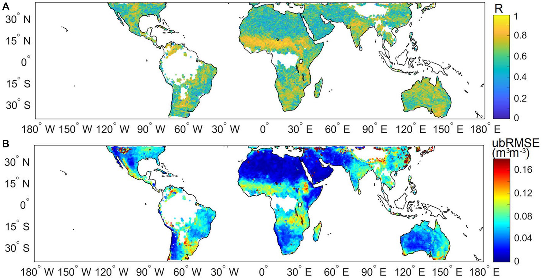
Figure 2. Correlation and ubRMSE of CYGNSS SM and SMAP SM in 2022 at 36-km grid, respectively.

SM is a critical component in climate change, and the working band of CYGNSS is capable of estimating SM under forest land types. The SM accuracy over forest regions and different climate types is assessed here. Table 1 shows the variation values of R and ubRMSE due to climate type. The climate types data is obtained from Köppen-Geiger Climate Classification dataset (Kottek et al., 2006). As illustrated in Table 1, the SM of the equatorial climate has the highest R values, and the ubRMSE of the arid climate outperforms other climate types. The number of valid CYGNSS SM is much less, which may lead to a relatively large statistical error. The forest cover types are obtained from International Geosphere Biosphere Programme (IGBP) data (Loveland et al., 2000). When the forest types are considered (Table 2), the R-value is larger than 0.5, but the correlation is lower than the global average R-value.

TABLE 1

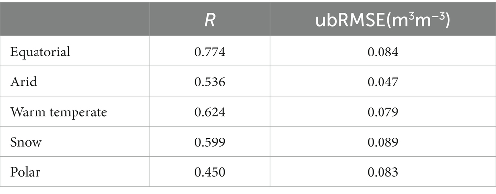
Table 1. The statistical indices for different climate types.

TABLE 2

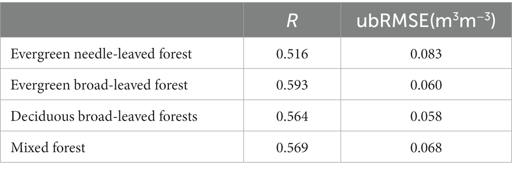
Table 2. The statistical indices for different forest types.

4.2 Correlations of CYGNSS SM and the NDVI

To investigate the linkage between the SM and vegetation, the 15-day average of the CYGNSS SM is used as the final value of SM, to match up with the NDVI data. A comparison of CYGNSS SM with NDVI from 2019.01 to 2022.12 is shown in Figure 3. The SMAP SM and NDVI comparison is also provided for comparison purposes (Figure 3B). As illustrated in Figure 3, the R-values vary considerably with different time grids, with R-values ranging from −1 to 1. The area ratio of positive correlation is about 58%. A significant negative correlation occurs in the north of Africa, and Northwestern Asia. The positive correlation is distributed in the center of Arica with soil drying; this may be because changes in SM precede changes in NDVI, meaning that SM leads the behavior of vegetation in this region. These results reflect a double-sided linkage between vegetation and SM. As for SMAP SM, the distribution of correlation is similar to the case of CYGNSS SM against NDVI. The results show that the driving effect of SM on vegetation activity is more obvious in arid regions, and CYGNSS SM can capture the above key information in correlation with NDVI. Although the R-values of CYGNSS SM and SMAP SM are numerically different, the two spatial characteristics show similarity, indicating that CYGNSS SM is reliable.

FIGURE 3

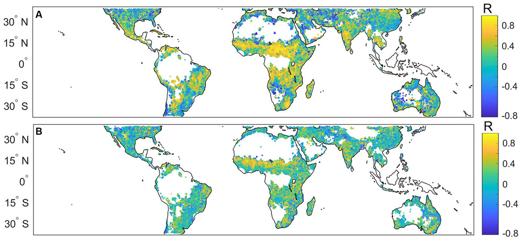
Figure 3. Correlations of CYGNSS SM and SMAP SM with NDVI from 2019.01 to 2022.12. (A) CYGNSS SM vs. NDVI, (B) SMAP SM vs. NDVI,

Boxplots of the R for thirteen IGBP land types of the CYGNSS SM and SMAP SM versus NDVI globally from January 2019 to December 2022 are shown in Figures 4A,B, respectively. Overall, the R-vales of all land types range from −1 to 1. The mean R-values of evergreen needleleaf forest, evergreen broadleaf forest, permanent wetlands, croplands/natural vegetation mosaic, and barren are smaller than 0. The results of SMAP SM versus NDVI show similarity with CYGNSS across different vegetation types, except for the barren type. NDVI mainly reflects the vegetation dynamics, while the NDVI of the areas is not representative, and the driving role of SM is difficult to explain. Therefore, it is not explored further in this study. Regarding vegetation types, forests have a greater capacity for water absorption by roots and are not sensitive to the response of SM, so even increases in SM in forested areas act as a slight inhibitor to vegetation growth. In contrast, the NDVI of the shrublands and grassland in relatively arid areas respond more significantly to SM. It is evident that SM also strongly controls vegetation growth here.

FIGURE 4

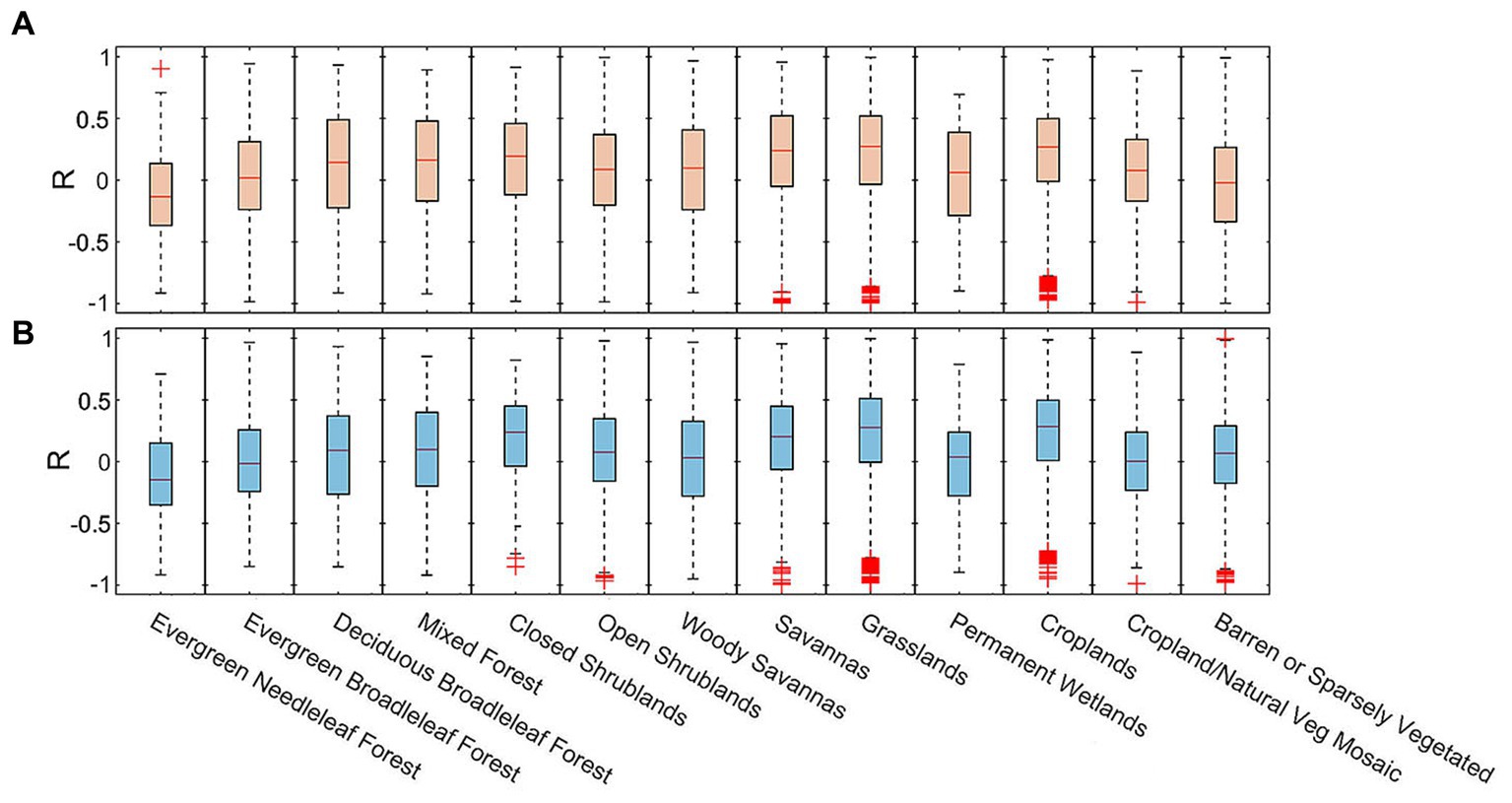
Figure 4. Boxplots of R for 13 land types in the period from August from 2019.01 to 2022.12. (A) CYGNSS SM vs. NDVI, (B) SMAP SM vs. NDVI.

4.3 Correlations of CYGNSS SM with the SOS

The R-values of annual CYGNSS SM and SOS for thirteen land cover types is obtained, as shown in Figure 5. Here, data from 10^o N to 38^o N are selected. CYGNSS SM from March to MAY is averaged to match up with the SOS data. Among the forest types, evergreen broadleleaf forests have the largest SM, corresponding to the earliest onset of spring phenology. Open shrublands, grasslands, croplands, and barren land have lower SM, and most of these vegetation types grow in relatively arid areas, corresponding to relatively low SM. These types correspond to larger SOS values. Accordingly, permanent wetlands and woody savannas show the maximum SM values, with the late emergence of spring phenology.

FIGURE 5

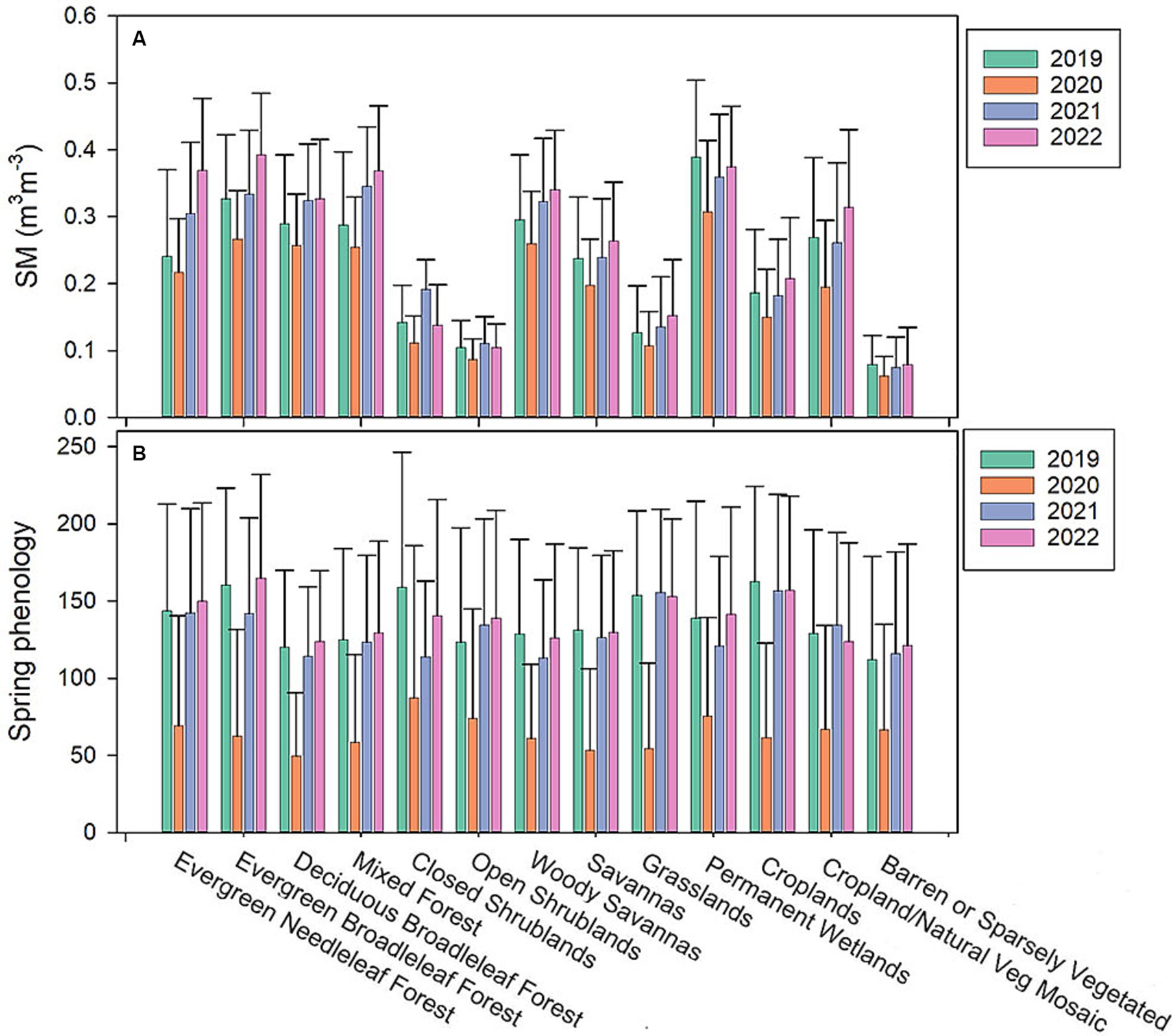
Figure 5. Distribution and mean CYGNSS SM and spring phenology each year. (A) mean CYGNSS SM, (B) start of spring phenology.

Figure 6 shows the heatmap of R-values of all the land cover types between the average SM and SOS values. Except for closed shrublands, all land cover types negatively correlated in 2019. For the evergreen needleleaf forest, the R-value gets larger each year, changing from a negative to a positive value. It illustrates that under the influence of SM, the SOS in evergreen needleleaf forests is increasingly later than the timing of SM changes. A stable negative correlation between SM and SOS in open shrublands and grasslands suggests that, correspondingly, SM contributes to vegetation green-up in arid regions under continued global warming.

FIGURE 6

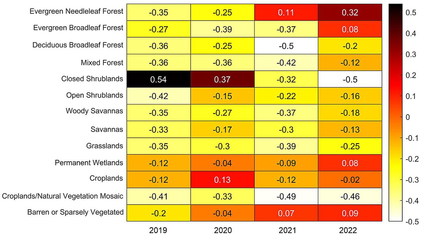
Figure 6. Correlation heatmap of all the land cover types between the average SM and SOS values from 2019 to 2022. Positive R-values are shown in red, and negative R-values are shown in yellow.

Although temperature has been the main driver of spring phenology under warming in recent decades (Shen et al., 2014), SM in arid regions becomes a critical limit for vegetation green-up. In addition, SOS and SM in deciduous broadleaf forests show a continuous negative correlation; thus, SM advances the SOS here. This may be related to the leaf structure of broadleaf forests. When spring begins, the temperature gradually rises. Evapotranspiration is the strongest in deciduous broadleaf forests, and the evaporated water is urgently needed for the cyclic process of continuous absorption of water by roots to recharge the trees. Thus, compared to the needleleaf forests and evergreen broadleaf forests in relatively humid environments, SOS in deciduous broadleaf forests and mixed forests are more significantly and consistently affected by SM.

5 Conclusion

In this study, the performance of CYGNSS SM is conducted with vegetation activity. The results of the study indicate that CYGNSS SM is important in the long term for large-scale terrestrial ecosystems and global change studies. There are obvious linkages between the CYGNSS and two key vegetation activity indexes (i.e., NDVI and the SOS). It indicates that the CYGSS SM can provide helpful information in response to changes in vegetation activity.

The results show that the CYGNSS SM with land surface and system error calibration correlates well with the SMAP SM (i.e., R = 0.693 vs. ubRMSE = 0.054 m³m⁻³). As for vegetation activity indexes, the correlation between the CYGNSS SM and NDVI varies considerably with different time grids, and the area ratio of positive correlation is about 58%. However, it shows a significant positive correlation in central Africa. The NDVI of the shrublands and grassland in relatively arid areas respond more significantly to SM. In terms of SOS, the correlations of SM and SOS display strong annual variations, and generally, the SM has experienced a significant negative effect on SOS, and SM advances the vegetation green-up in arid and semi-arid areas.

Foreseeably, the findings of this study can help understand the link between SM and vegetation activity in the pan-tropical region, and to better understand the impacts of climate change.

Data availability statement

The original contributions presented in the study are included in the article/supplementary material, further inquiries can be directed to the corresponding author.

Author contributions

TY: Formal analysis, Methodology, Validation, Writing – original draft, Writing – review & editing. NC: Writing – review & editing.

Funding

The author(s) declare financial support was received for the research, authorship, and/or publication of this article. This study is supported by the National Natural Science Foundation of China projects (Grant No. 42101376, 42071133).

Conflict of interest

The authors declare that the research was conducted in the absence of any commercial or financial relationships that could be construed as a potential conflict of interest.

Publisher’s note

All claims expressed in this article are solely those of the authors and do not necessarily represent those of their affiliated organizations, or those of the publisher, the editors and the reviewers. Any product that may be evaluated in this article, or claim that may be made by its manufacturer, is not guaranteed or endorsed by the publisher.

References

Chan, S. K., Bindlish, R., O'Neill, P. E., Njoku, E., Jackson, T., Colliander, A., et al. (2016). Assessment of the SMAP passive soil moisture product. IEEE Trans. Geosci. Remote Sens. 54, 4994–5007. doi: 10.1109/TGRS.2016.2561938

CrossRef Full Text | Google Scholar

Chang, J. T., and Wetzel, P. J. (1991). Effects of spatial variations of soil moisture and vegetation on the evolution of a prestorm environment: a numerical case study. Mon. Weather Rev. 119, 1368–1390. doi: 10.1175/1520-0493(1991)119<1368:EOSVOS>2.0.CO;2

CrossRef Full Text | Google Scholar

Chen, A., Meng, F., Mao, J., Ricciuto, D., and Knapp, A. K. (2022). Photosynthesis phenology, as defined by solar-induced chlorophyll fluorescence, is overestimated by vegetation indices in the extratropical northern hemisphere. Agric. For. Meteorol. 323:109027. doi: 10.1016/j.agrformet.2022.109027

CrossRef Full Text | Google Scholar

Chew, C., Shah, R., Zuffada, C., Hajj, G., Masters, D., and Mannucci, A. J. (2016). Demonstrating soil moisture remote sensing with observations from the UK TechDemoSat-1 satellite mission. Geophys. Res. Lett. 43, 3317–3324. doi: 10.1002/2016GL068189

CrossRef Full Text | Google Scholar

Chew, C. C., and Small, E. E. (2018). Soil moisture sensing using spaceborne GNSS reflections: comparison of CYGNSS reflectivity to SMAP soil moisture. Geophys. Res. Lett. 45, 4049–4057. doi: 10.1029/2018GL077905

CrossRef Full Text | Google Scholar

Chew, C., and Small, E. (2020). Description of the UCAR/CU soil moisture product. Remote Sens. 12:1558. doi: 10.3390/rs12101558

CrossRef Full Text | Google Scholar

Choudhury, B. J., Schmugge, T. J., Chang, A., and Newton, R. W. (1979). Effect of surface roughness on the microwave emission from soils. J. Geophys. Res. Oceans 84, 5699–5706. doi: 10.1029/JC084iC09p05699

CrossRef Full Text | Google Scholar

Cong, N., Piao, S., Chen, A., Wang, X., Lin, X., Chen, S., et al. (2012). Spring vegetation green-up date in China inferred from SPOT NDVI data: a multiple model analysis. Agric. For. Meteorol. 165, 104–113. doi: 10.1016/j.agrformet.2012.06.009

CrossRef Full Text | Google Scholar

Dong, J., Crow, W. T., Tobin, K. J., Cosh, M. H., Bosch, D. D., Starks, P. J., et al. (2020). Comparison of microwave remote sensing and land surface modeling for surface soil moisture climatology estimation. Remote Sens. Environ. 242:111756. doi: 10.1016/j.rse.2020.111756

CrossRef Full Text | Google Scholar

Eroglu, O., Kurum, M., Boyd, D., and Gurbuz, A. C. (2019). High spatio-temporal resolution CYGNSS soil moisture estimates using artificial neural networks. Remote Sens. 11:2272. doi: 10.3390/rs11192272

CrossRef Full Text | Google Scholar

Foti, G., Gommenginger, C., Jales, P., Unwin, M., Shaw, A., Robertson, C., et al. (2015). Spaceborne GNSS reflectometry for ocean winds: first results from the UK TechDemoSat-1 mission. Geophys. Res. Lett. 42, 5435–5441. doi: 10.1002/2015GL064204

CrossRef Full Text | Google Scholar

Gleason, S., Ruf, C. S., O’Brien, A. J., and McKague, D. S. (2018). The CYGNSS level 1 calibration algorithm and error analysis based on on-orbit measurements. IEEE J. Sel. Top. Appl. Earth Obs. Remote Sens. 12, 37–49. doi: 10.1109/JSTARS.2018.2832981

CrossRef Full Text | Google Scholar

Jing, C., Niu, X., Duan, C., Lu, F., Di, G., and Yang, X. (2019). Sea surface wind speed retrieval from the first Chinese GNSS-R mission: technique and preliminary results. Remote Sens. 11:3013. doi: 10.3390/rs11243013

CrossRef Full Text | Google Scholar

Kottek, M., Grieser, J., Beck, C., Rudolf, B., and Rubel, F. (2006). World map of the Köppen-Geiger climate classification updated, Meteorol. 15, 259–263. doi: 10.1127/0941-2948/2006/0130

CrossRef Full Text | Google Scholar

Luo, M., Meng, F., Sa, C., Duan, Y., Bao, Y., Liu, T., et al. (2021). Response of vegetation phenology to soil moisture dynamics in the Mongolian Plateau. Catena 206:105505.

Google Scholar

Loveland, T. R., Reed, B. C., Brown, J. F., Ohlen, D. O., Zhu, Z., Yang, L. W. M. J., et al. (2000). Development of a global land cover characteristics database and IGBP DISCover from 1 km AVHRR data. Int. J. Remote Sens. 21, 1303–1330. doi: 10.1080/014311600210191

CrossRef Full Text | Google Scholar

Piao, S., Fang, J., Zhou, L., Ciais, P., and Zhu, B. (2006). Variations in satellite-derived phenology in China's temperate vegetation. Glob. Chang. Biol. 12, 672–685. doi: 10.1111/j.1365-2486.2006.01123.x

CrossRef Full Text | Google Scholar

Ruf, C. S., Chew, C., Lang, T., Morris, M. G., Nave, K., Ridley, A., et al. (2018). A new paradigm in earth environmental monitoring with the cygnss small satellite constellation. Sci. Rep. 8:8782. doi: 10.1038/s41598-018-27127-4

PubMed Abstract | CrossRef Full Text | Google Scholar

Ruf, C., Unwin, M., Dickinson, J., Rose, R., Rose, D., Vincent, M., et al. (2013). CYGNSS: enabling the future of hurricane prediction [remote sensing satellites]. IEEE Trans. Geosci. Remote Sens. 1, 52–67. doi: 10.1109/MGRS.2013.2260911

CrossRef Full Text | Google Scholar

Shen, M., Tang, Y., Chen, J., Yang, X., Wang, C., Cui, X., et al. (2014). Earlier-season vegetation has greater temperature sensitivity of spring phenology in northern hemisphere. PLoS One 9:e88178. doi: 10.1371/journal.pone.0088178

PubMed Abstract | CrossRef Full Text | Google Scholar

Wan, W., Ji, R., Liu, B., Li, H., and Zhu, S. (2020). A two-step method to calibrate CYGNSS-derived land surface reflectivity for accurate soil moisture estimations. IEEE Geosci. Remote Sens. Lett. 19, 1–5. doi: 10.1109/LGRS.2020.3023650

CrossRef Full Text | Google Scholar

Yan, Q., Huang, W., Jin, S., and Jia, Y. (2020). Pan-tropical soil moisture mapping based on a three-layer model from CYGNSS GNSS-R data. Remote Sens. Environ. 247:111944. doi: 10.1016/j.rse.2020.111944

CrossRef Full Text | Google Scholar

Yang, G., Bai, W., Wang, J., Hu, X., Zhang, P., Sun, Y., et al. (2022a). FY3E GNOS II GNSS reflectometry: Mission review and first results. Remote Sens. 14:988. doi: 10.3390/rs14040988

CrossRef Full Text | Google Scholar

Yang, T., Wan, W., Wang, J., Liu, B., and Sun, Z. (2022b). A physics-based algorithm to couple CYGNSS surface reflectivity and SMAP brightness temperature estimates for accurate soil moisture retrieval. IEEE Trans. Geosci. Remote Sens. 60, 1–15. doi: 10.1109/TGRS.2022.3156959

CrossRef Full Text | Google Scholar

Zhao, F., Wang, X., Wu, Y., Sivakumar, B., and Liu, S. (2023). Enhanced dependence of China’s vegetation activity on soil moisture under drier climate conditions. J. Geophys. Res. Biogeosci. 128:e2022JG007300. doi: 10.1029/2022JG007300

CrossRef Full Text | Google Scholar