Abstract
Thinning practices have increased to maintain healthy and resilient forests. However, there is a growing concern about the potential effects of thinning on hydrological response. We analyzed the influence of thinning on shallow soil water flux in a mixed conifer forest by comparing paired treated and control plots. Sensors measured soil volumetric water content and soil matric potential at different depths to compute soil water fluxes over five seasons. Additionally, we analyzed soil temperature and soil volumetric water content data. Thinning treatment led to upward soil water flux during the study period (2009–2011), regardless of the season. This was mainly due to differences in soil gradients, possibly associated with an increased soil temperature by as much as 2.65 °C due to increased solar radiation. Although thinning increased upward water flux (< 0.2 mm day−1), it constituted a negligible part of the soil volumetric water content stored in thinned plots, which was 0.15 cm3 cm−3 greater, at 35 cm depth, than in control plots. Our findings suggest that thinning can contribute to soil moisture storage even during dry periods, likely stored at the bottom of the soil column on a rock surface. Thinning can have a positive impact on the resilience of forests to droughts and other climate-related stresses.
1 Introduction
Thinning, as a tool for vegetation management, helps maintain healthy and resilient forests, although it may modify the hydrological processes. In 1965, forest hydrology emerged as a discipline to understand the hydrological responses of thinned stands (Sopper and Lull, 1967). The Wagon Wheel Gap was the first paired watershed study to evaluate (i.e., before and after) the response of forest removal on stream and erosion. The results showed an increased water yield in the thinned watershed vs. the control watershed. However, water yield diminished 7 years after treatment (McGuire and Likens, 2011).
Forest thinning effects have been widely reported for water use (Park et al., 2018), water infiltration (Di Prima et al., 2017), soil moisture (Belmonte et al., 2022), soil water-holding capacity (Wang et al., 2021), soil carbon stocks and dynamics (Zhang et al., 2018), soil-plant dynamics (Bai et al., 2017), and runoff and sediment yield (Garduño et al., 2015; Yang et al., 2019). Research reported about the effects of thinning and slash scattering or pile has demonstrated that runoff and sediment yield might be diminished due to soil protection (Cram et al., 2007; Atalar et al., 2021), yet the soil moisture was similar under these treatments (Madrid et al., 2006). del Campo et al. (2022) reported a meta-analysis of thinning influences on the hydrologic process. This review encompassed forest-thinning experiments mainly carried out in North America and Europe. For instance, at the stand level, stemflow and stand transpiration were lower with the thinning treatment, whereas soil moisture, tree-level water use, and sap flow increased for individual trees left after the thinning treatment. Thinning had no significant effect on total evapotranspiration. None of the reported experiments addressed the soil water flux. While few studies have measured the soil water potential, the driver of flux, in tropical and temperate forests (Kupers et al., 2019a,b; Courcot et al., 2024), little research on thinned semiarid forests has been reported (Tatum et al., 2025). The need for more in-situ data was emphasized as a research priority by Novick et al. (2022). Although thinning effects on soil water storage are predictable, how it alters the movement of water through shallow soils is still uncertain.
This subsurface water flow is the key process that connects changes in surface water input to deeper hydrological functions, including the water stored in the underlying weathered bedrock (Salve et al., 2012). In forestlands, the underlying weathered bedrock allows the water transport and retention into the fractures (Liu et al., 2025). The unsaturated weathered bedrock (Zhang and Zhang, 2021) is recognized as an important water reservoir known as “rock moisture,” which can support water storage for tree water uptake and groundwater recharge (Liu et al., 2025; Salve et al., 2012).
The water movement (hereafter, “water flux”) in a porous system occurs in the saturated or unsaturated zone. Water flows in the saturated zone by positive potentials (Lal and Shukla, 2004) and by negative potentials in the unsaturated zone (i.e., above the water table) (Domenico and Schwartz, 1997). In the unsaturated zone, water movement is vertically downward due to gravitational forces and can be in any direction based on water potential caused primarily by capillary potential gradients (Lee, 1980). However, water movement in the unsaturated zone is limited by unsaturated hydraulic conductivities, especially in dry soils (Lal and Shukla, 2004). The direction of flow is given by the direction of the gradient (elevation head) (z) + soil water potential (ψ) (Bond, 1998). In forest soils, soil water flux is controlled by precipitation and evaporation (Löffler, 2007; Xu et al., 2012). Harr (1977) reported that soil water flux at a depth of 0–30 cm was in downslope (i.e., horizontal) direction between storms and in both downward (i.e., vertical) and downslope directions during storms.
In the unsaturated zone, nutrients and water are stored for plant consumption. This zone purifies water (e.g., removes chemical and biological contaminants) and provides nutrients for plant consumption (Flury and Wai, 2003). The available groundwater occurs by deep percolation through the unsaturated zone (Dingman, 2008). Forests exert influence on soil water storage by evapotranspiration and discharging water. Evapotranspiration uses water from shallow or deep layers, resulting in the withdrawal of soil water (Lee, 1980), creating a soil moisture deficit that impacts water storage and consequently the water balance. Recharge occurs when deep percolation reaches the adjacent saturated zone (i.e., the movement of percolating water from the unsaturated to the saturated zone), as well as in vertical or horizontal seepage from surface water bodies (Dingman, 2008).
Recognizing these processes is critical in climate change concerns, as shifts in precipitation patterns and increased temperatures can further impact evapotranspiration rates, soil moisture dynamics, and ecosystem water balance. These shifts in patterns are likely to be experienced in the southwestern US forests, where mixed montane forests are moderately to highly vulnerable to climate change (Thorne et al., 2018). The Southwest North America region has experienced a “megadrought” since the 21st century (Williams et al., 2022). Changes in precipitation patterns and rising temperatures are the drivers of such drying (Maloney et al., 2014; Cook et al., 2015). Climate models suggest that, by the 2030s, summer soil moisture conditions could either shift toward a wetter regime than the current megadrought (though still drier than the 1980s−1990s precipitation) or, in the most extreme case, worsen beyond 21st-century megadrought (Seager et al., 2023). Given the Southwest's vulnerability to climate-driven drying, it is important to analyze how thinning overstocked forest stands influences hydrological response.
There is a lack of understanding of shallow soil water dynamics after forest thinning. The designed study measured the effects of masticator thinning on the soil water flow in mixed conifer forest stands in the southwestern United States. We hypothesized that “Within each season, water flux and soil volumetric water content means will differ between forests thinned with scattered slash and untreated control forests.” We expect that for water flux, this primary hypothesis translates into treated plots having downward flux during seasons when water input through snowmelt and rainfall is highest. During the low water input (dry season), we expect that treated plots may have upward flux. This study offers a novel analysis of 2.8 years of soil water flux data, providing valuable information to land and water managers seeking to thin overstocked mixed conifer stands under climate-related stress.
2 Materials and methods
2.1 Description of the study site
The study site is located in the southern Sacramento Mountains near the village of Cloudcroft, NM. Elevations are 2,127 m in the valley site and 2,748 m on the ridge (Figures 1A–C). The climate is considered warm-dry (Fulé et al., 2009), with a mean monthly temperature of 22 °C in July and 5 °C in January, and a mean annual precipitation of 752 mm (1987–2016; WRCC). Topography is steep, with most slopes ranging from 20 to 40%, and shallow soils approximately 35 cm deep, consisting of clay and clay loam textures (Garduño et al., 2015). The average wilting point (Wp), field capacity (Fc), and hydraulic conductivity (Kh) are shown in Table 1. The soil type is Typic Argiborolls-Aquic Haploborolls. The experimental watershed lies above the Permian San Andres and upper Yeso formations. A complex hydrological system is influenced by exposed geological features and regional fracture systems. This system enables rapid movement of much of the high-altitude precipitation through interconnected shallow carbonate aquifers perched and linked by fracture networks and surface water drainages (Newton et al., 2015).
Figure 1
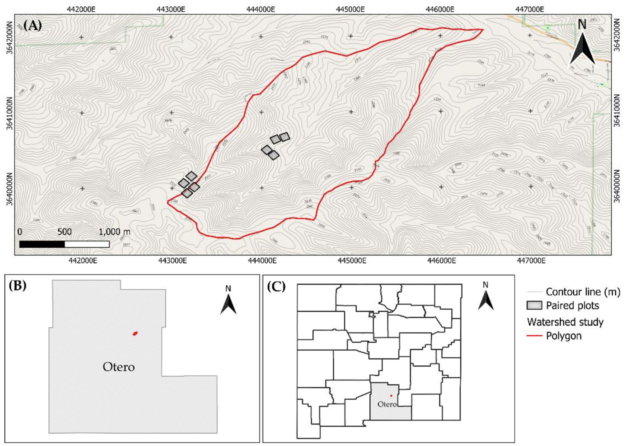
Location of the study site. (A) Watershed study area showing paired plots, (B) location of the study site in Otero County within the State of New Mexico (C).
Table 1
| Depth (cm) | Control | Thinned | ||
|---|---|---|---|---|
| Wp * (cm 3 cm −3 ) | Fc * (cm 3 cm −3 ) | Wp (cm 3 cm −3 ) | Fc (cm 3 cm −3 ) | |
| 7 | 0.110 | 0.327 | 0.075 | 0.330 |
| 20 | 0.102 | 0.267 | 0.130 | 0.450 |
| 35 | 0.087 | 0.385 | 0.077 | 0.417 |
| Ks * (cm day −1 ) | ||||
| 7 | 5.695 | 5.848 | ||
| 20 | 7.003 | 7.138 | ||
| 35 | 7.335 | 6.255 | ||
Average soil hydraulic properties of the study site at different depths.
*Wp is the wilting point, Fc is the field capacity, and Ks is the saturated hydraulic conductivity.
The overstory community is dominated by Douglas fir (Pseudotsuga menziesii Mirb.) and ponderosa pine (Pinus ponderosa C. Lawson). The understory herbaceous community is dominated by Stipa and Sporobolus species, Alder leaf mountain-mahogany (Cercocarpus montanus Raf.), and Longflower snowberry (Symphoricarpos longiflorus A. Gray) (Garduño et al., 2015). The height of trees, diameter at breast height (DBH), and density ranged from 6 to 13 m, 10 to 25 cm, and 80 to 159 trees ha−1, respectively (Table 2).
Table 2
| Landscape | Plot | Treatment | Zveg | DBH | Density | CC (%) | Aspect | Slope | Soil | |
|---|---|---|---|---|---|---|---|---|---|---|
| Position | pair | (m) | (cm) | Trees ha −1 | Pre-trt | Post-trt | (%) | texture | ||
| Ridge | 1 | Control | 8 | 14.5 | 159 | 51 | 51 | North | 24 | Clay Loam |
| Thinned | 7.4 | 14.3 | 146 | 61 | 1 | North | 18 | Loam | ||
| 2 | Control | 6.3 | 10.5 | 115 | 99 | 99 | South | 19 | Clay Loam | |
| Thinned | 7.2 | 12.5 | 159 | 90 | 11 | South | 21 | Loam | ||
| Valley | 3 | Control | 9.5 | 24.4 | 90 | 98 | 98 | North | 21 | Loam |
| Thinned | 12.9 | 24.4 | 80 | 99 | 81 | North | 12 | Clay Loam | ||
| 4 | Control | 9.3 | 20.03 | 58 | 61 | 61 | South | 28 | Loam | |
| Thinned | 8.9 | 17.36 | 85 | 90 | 25 | South | 16 | Loam | ||
Characterization of paired plots at the study site.
Zveg is the height of trees, DBH the diameter at breast height, Cc the canopy cover. For cover, pre-trt was calculated in May 2009 and post-trt was calculated in May 2010. Zveg, DBH, and Density were calculated before the thinning experiment.
2.2 Thinning treatment
In mid-August 2009, one randomly selected plot was thinned from each of four experimental plot pairs (8,100 m2 or a dimension of 90 m × 90 m each plot) (Figure 2). The thinning was performed using a boom-mounted masticator attached to a Caterpillar 320D LLR Hydraulic excavator (23,700 kg weight), which shredded trees from the top to the base. The resulting slash (i.e., bark and branches) was left on site (Supplementary Figure 1A). The other plot within a pair was left as an untreated control plot. Within plot pairs (i.e., blocks), the treatment and the control plot had similar aspects (north or south). Two plot pairs were installed on the ridge and two on the valley (Supplementary Figure 1A). This blocking design with four replicates (two in the ridge and two in the valley) is robust for detecting treatment effects. However, the limited number of blocks may constrain the spatial extrapolation of the findings to landscapes with greater topographic complexity.
Figure 2
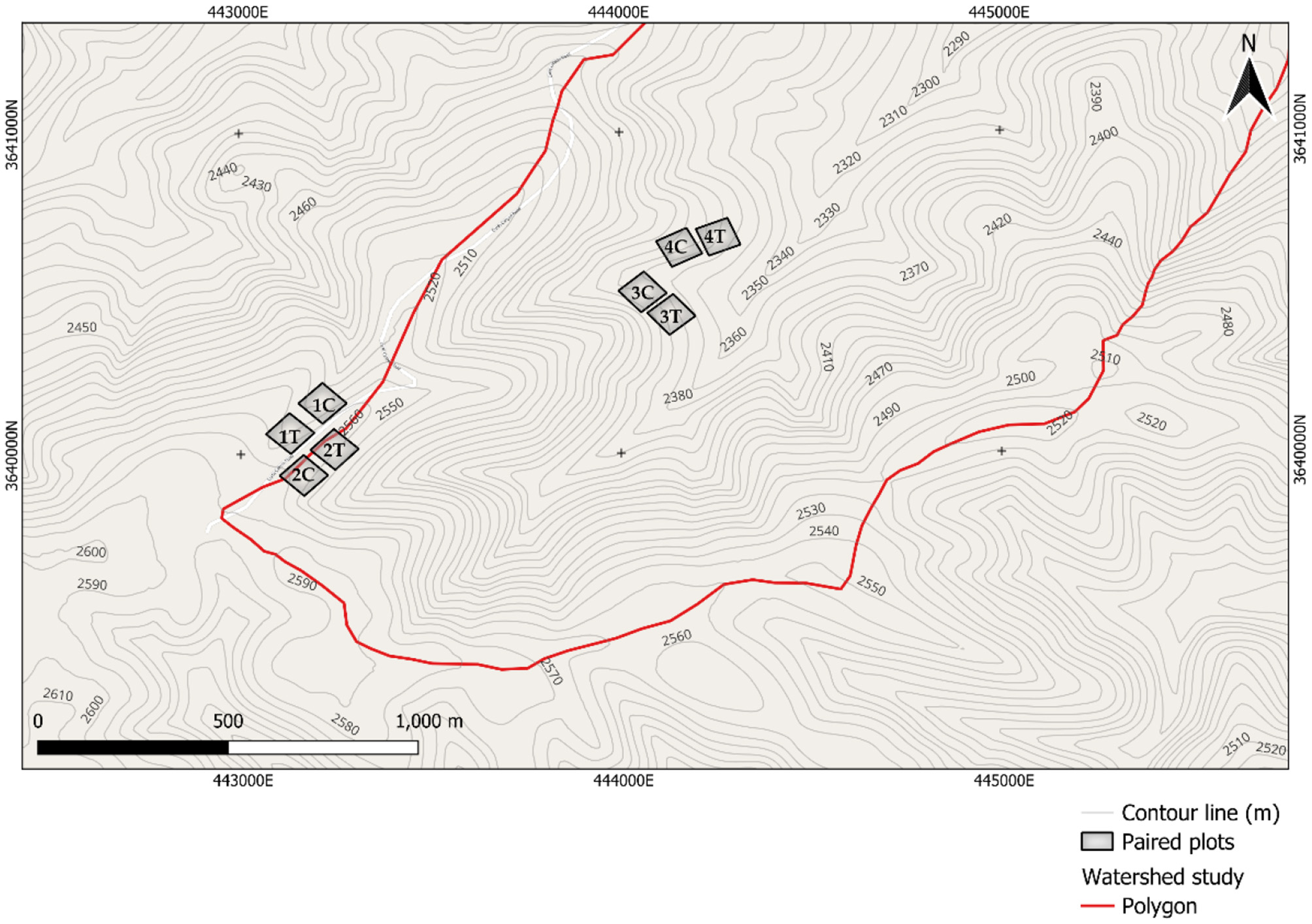
The watershed study area shows paired plots at the ridge (1 and 2) and the valley (3 and 4). Letters within plots indicate thinned plots (T) and control plots (C).
On control plots, pine needles and litter covered the soil, ranging from 46.81 to 95.29% with a depth of 1.27 to 4.43 cm. Pre-treatment canopy cover (i.e., calculated with the Normalized Difference Vegetation Index) on selected thinned plots averaged 85 and 77 % in control plots. Post-treatment canopy cover averaged 30% with slash depth ranging from 1 to 7 cm (Garduño et al., 2015).
2.3 Field data collection
2.3.1 Precipitation
Two tipping-bucket rain gauges (NovaLynx Corporation, Grass Valley, CA) were installed in the study area. One rain gauge was installed in the ridge landscape position in plot pair one between the control and thinned plots. The second rain gauge was in the valley landscape position, approximately 20 m from plot pair three and 25 m from plot pair four. Rain gauges recorded hourly data from January 2009 through October 2011.
2.3.2 Soil volumetric water content and soil temperature
Soil volumetric water content (θ) and soil temperature (Ts) were measured by ECHO2-EC-TM sensors (Decagon Devices, 2008, Pullman, WA). A set of three sensors per plot was installed in September 2008 to a depth of 7, 20, and 35 cm on each plot (Supplementary Figure 2). Sensors measured changes in the soil dielectric permittivity of the surrounding medium. Each specific soil type was unique and required calibration to determine absolute values of θ. Calibration was done following Decagon Devices procedures (Cobos and Chambers, 2009). The linear regression obtained from the calibration was used to convert θ from raw counts or raw data (Supplementary Figure 3). Soil temperature was measured in degrees Celsius with a thermistor underneath the probe overmold. The thermistor is in thermal contact with the probe prongs and reads the temperature along the prong surface of 5.2 cm long. Temperature data did not require calibration (Decagon Devices, 2008). Soil volumetric water content and Ts data were recorded hourly and reported daily from January 2009 through October 2011.
2.3.3 Air and slash temperature
The air temperature was measured at a two-meter height in plot pair one between the control and thinned plots (ridge site). The second sensor was installed in the control plot in plot pair three (valley site). These sensors were housed in a 6-plate Gill Radiation Shield model 41303-5A (Campbell Scientific, Logan, UT) to keep the probe at or near ambient temperature. The slash cover temperature was measured at a two-centimeter height in each thinned plot over the study period (n = 4) (Supplementary Figure 2). These sensors were housed in an oval mesh to keep out rodents. Air and slash temperature data were recorded hourly and reported daily from October 2009 through October 2011.
2.3.4 Soil water potential
Soil water potential (Ψ) was calculated using heat dissipation sensors model 229 (Campbell Scientific, Logan, UT). The sensors were installed at depths of 7, 20, and 35 cm on each plot during the last week of April 2009 (Figure 3). The soil matric potential was indirectly measured based on the heat dissipation method. Before installation, heat dissipation sensors were individually calibrated in the laboratory by the pressure extractor method (Campbell Scientific, 2006; Supplementary Figure 4).
Figure 3
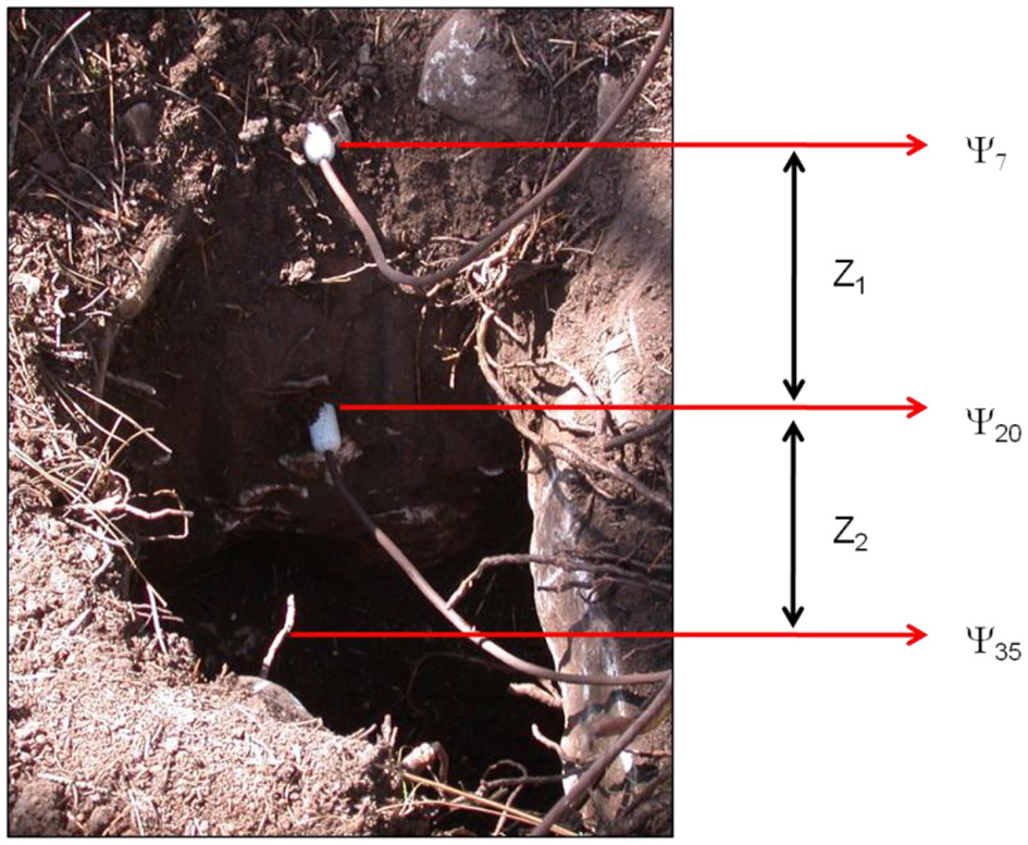
Installation of heat dissipation sensors at multiple soil depths for monitoring soil water potential. The symbol Ψ represents the matric potential, while the letter Z denotes the gravitational potential. Depth 1 (Z1) refers to data obtained at 7 and 20 cm, and depth 2 (Z2) corresponds to data obtained at 20 and 35 cm.
Soil volumetric water content, Ts, and Ψ were measured on each plot concurrently within 50 cm of each other at four plot pairs at the ridge and valley landscape position from January 2009 through October 2011. Soil volumetric water content and heat dissipation sensors were installed between three or four trees without touching the gravel or roots. After thinning, sensors did not have any influence on tree roots nearby. In control plots, tree roots might influence sensors. All sensors deployed were packed with soil and covered with needle pines or slash, depending on the treatment.
2.4 Soil water retention curve (SWRC)
The soil water retention curve was used to calculate the soil volumetric water content at field capacity, θfc, and permanent wilting point, θpwp (Supplementary Table 1). Mean daily values of ψ and θ were used to generate SWRC for each depth and site. Soil ψ and θ were screened for outlying values, which were removed from the subsequent curve analyses. After the screening process, ψ was converted to cm of H2O by multiplying MPa by 10197. Then, the soil particle size distribution data, ψ and θ were used as input data to calculate the SWRC for each plot at each depth. The Retention Curve program (RETC, Version 6.02) was used to fit the SWRC using the van Genuchten model described by
Where s is the effective degree of saturation, α, k (equivalent to the van Genuchten shape parameter n), and m are empirical constants affecting the shape of the retention curve (Supplementary Table 1). For further information, (see van Genuchten, 1980). Equation 1 was selected for fitting the SWRC because it performs best for many soils (van Genuchten et al., 1991). Unsaturated hydraulic conductivity (K) was calculated for each depth using Gardner's equation (Gardner, 1958) described by
Where n is the porosity, a and b are constants estimated by hydraulic properties (Campbell, 2008) described by
Where lnθpwp is the natural logarithm of the wilting point, lnθfc is the natural logarithm at field capacity of the soil volumetric water content (cm3 cm−3) for each soil at each depth determined with the RETC program. Although hysteresis can significantly influence water flux, it was not considered in describing water flux, as no unique functional relationship can be easily assumed (Weiler and McDonnell, 2004).
2.4.1 Shallow soil water flux
Shallow soil water flux (q) was determined at two depths: (1) 7 to 20 cm and (2) 20 to 35 cm according to Darcy's law (Hanks, 1992) and modified by Richards, who added +1 to account for the gravitational potential in unsaturated soils (Richards, 1931) described by
Where K(ψ) is the unsaturated hydraulic conductivity (cm day−1) as a function of matric potential at a known depth, Δh is the hydraulic gradient (cm cm−1) difference between two depths, and ΔZ is the difference in potential between two depths (cm).
Each hydraulic head is described by
Substituting Equation 5 into Equation 4 water flux was calculated as follows:
The reference level for gravitational potential (z) is the soil surface, and the positive z-axis is directed upward. Negative water flux (-q) indicates downward water flux, and positive flux (q) indicates upward water flux (mm day−1).
2.5 Data analysis
Soil temperature, soil volumetric water content, and water flux were analyzed by depth using a mixed model with fixed effects for treatment, month, and their interaction, but focused on two-tailed pre-planned comparisons of control-treatment differences within specific seasons. To allow considering a relatively flexible set of parsimonious candidate covariance structures, we fitted covariance structures with random pair × month effects, and different combinations of random plot effects (uniquely identified as pair × treatment) and AR (1) (autoregressive) variance structures fit pooling across treatment or separately by treatment. We based formal inference on the covariance structure with the lowest AICc (Akaike Information Criteria). We conducted 12 pre-planned comparisons of treatment to control by averaging across the months in the indicated seasons. Seasons fell into the following five categories, with all but the pre-treatment season corresponding to multiple pre-planned comparisons for each incidence of that season over the 2009-2011 study years. (1) The pre-treatment season (May-August 2009); (2) The dry season fall (October) and spring (May); (3) The snow season (November–January); (4) The snowmelt season (March–April); and (5) The rainy season (June–September). We assessed the sensitivity of the findings to the specific model chosen and to outliers by fitting the two models with the lowest two AICc values with and without extreme outliers, defined as those observations with marginal studentized residual values of magnitudes exceeding 4. Reported results are based on the specific model chosen, noting when findings were sensitive to either the alternative model or outliers. We defined significance as α ≤ 0.05 and conducted analyses using SAS (version 9.4−2006 ® SAS Institute Inc).
3 Results
3.1 Precipitation
Based on the Cooperative Climatological Data Summaries of precipitation data covering 30 years, the highest precipitation was in July, followed by August, while the driest month was April, followed by May (Table 3). For 2009, 2010, and 2011, the total annual precipitation recorded was 238, 408, and 159 mm, respectively. The lowest monthly precipitation of 1 mm was recorded in November 2010, March, and April 2011, while the highest monthly precipitation of 140 mm occurred in July 2010 (Table 3). The rainy season was marked by a different precipitation regime throughout the study period (2009–2011). The lowest precipitation, during the rainy season, was recorded in 2011 (140 mm), while the highest precipitation of 299 mm was recorded in 2010; 2009 was in the middle of this precipitation regime with 169 mm. Examining the seasonal distribution of precipitation (1987–2016), it was observed that the study period (2009–2011) coincided with a drought phase. This period was characterized by a reduction in monthly precipitation amount, evident in the overall seasonal distribution of precipitation.
Table 3
| Precipitation (mm) | |||||
|---|---|---|---|---|---|
| Season | Month | 1987–2016 ** | 2009 | 2010 | 2011 |
| Snow | January | 41 | - | 15 | 5 |
| February | 48 | - | 0 | 12 | |
| Snowmelt | March | 34 | - | 3 | 1 |
| April | 22 | - | 9 | 1 | |
| Dry | May | 33 | 62* | 13 | 0 |
| Rainy | June | 58 | 46* | 38 | 3 |
| July | 151 | 79* | 140 | 42 | |
| August | 144 | 25* | 87 | 68 | |
| September | 79 | 19 | 34 | 28 | |
| Dry | October | 50 | 7 | 19 | 0 |
| Snow | November | 37 | 25 | 1 | - |
| December | 55 | 19 | 4 | - | |
Monthly average precipitation (1987–2016) and monthly precipitation (2009–2011).
*Pre-treatment season.
**29-year monthly average (Source from Western Regional Climate Center (WRCC) (2024). Cooperative Climatological Data Summaries).
The dash symbol indicates missing data.
3.2 Slash cover and air temperature
The variability of slash cover temperature and air temperature followed a seasonal trend characterized by a gradual rise and decline according to the seasons. The highest slash cover temperature and air temperature were recorded in June 2011 (22 °C and 21 °C, respectively). The lowest slash cover temperature and air temperature below zero were obtained from December 2009 through February 2010, except for January, with an air temperature above zero (Figure 4).
Figure 4
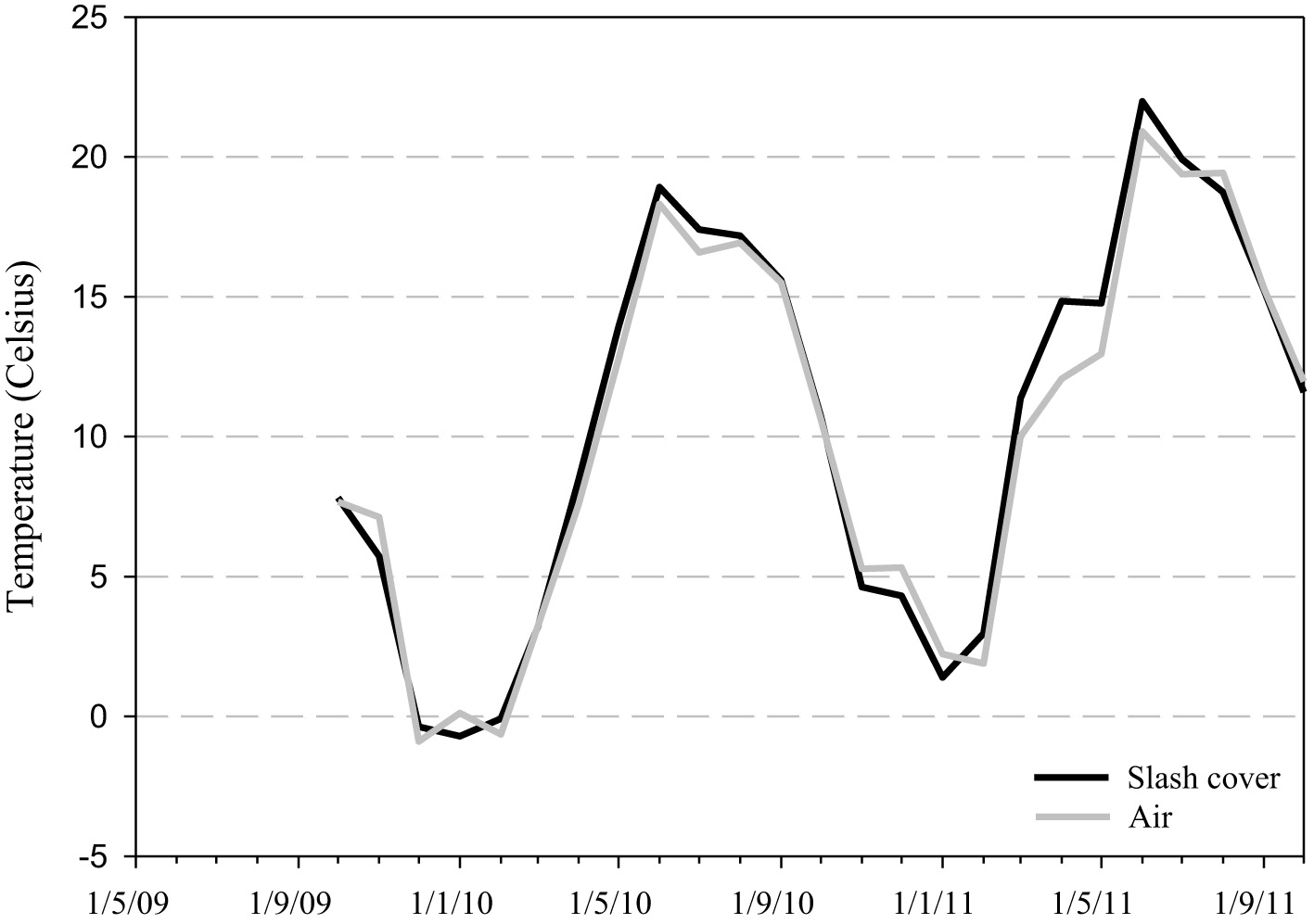
Monthly average slash cover temperature and air temperature.
3.3 Soil temperature (Ts)
The soil temperature at 7 cm depth was higher in the thinned plots as compared to the control plots. The difference was statistically significant from May 2010 (dry season) through the rainy season of 2010, with differences of 2.65 ± 1.07 °C and 2.15 ± 0.96 °C, respectively (Figure 5). At 20 cm depth, temperatures in the thinned plots were higher than those observed for the control plots from snowmelt until October (fall dry season). The difference was statistically significant in May 2011 (dry season), rainy 2011, and October 2011 (fall dry season), with the estimated difference between treated and control plots being 2.50 ± 1.09 °C, 2.62 ± 0.99 °C, and 2.49 ± 1.09 °C, respectively (Figure 5). At 35 cm depth, no significant differences were observed between thinned and control plots (Figure 5).
Figure 5
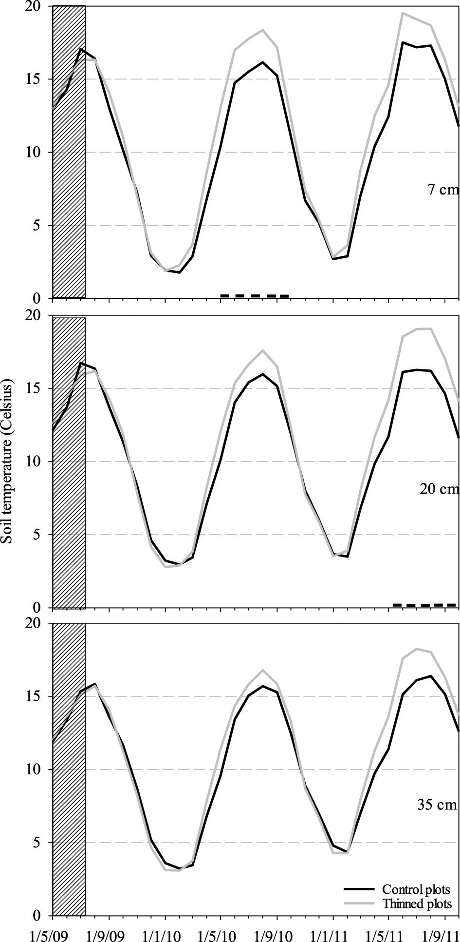
Monthly average soil temperature at three different depths. The statistical significance is represented by the black bold minus symbol. The vertical rectangle (hatched area) depicts the pre-treatment season.
3.4 Soil volumetric water content (θ)
At the 7 cm depth, θ was similar between the thinned and control plots (Figure 6). Both treatments showed a sharp decrease in θ approaching to wilting point of 0.07 cm3 cm−3 (thinned plots) and 0.11 cm3 cm−3 (control plots). On the other hand, thinned plots approached field capacity (0.32 cm3 cm−3) during the snowmelt season in March 2010.
Figure 6
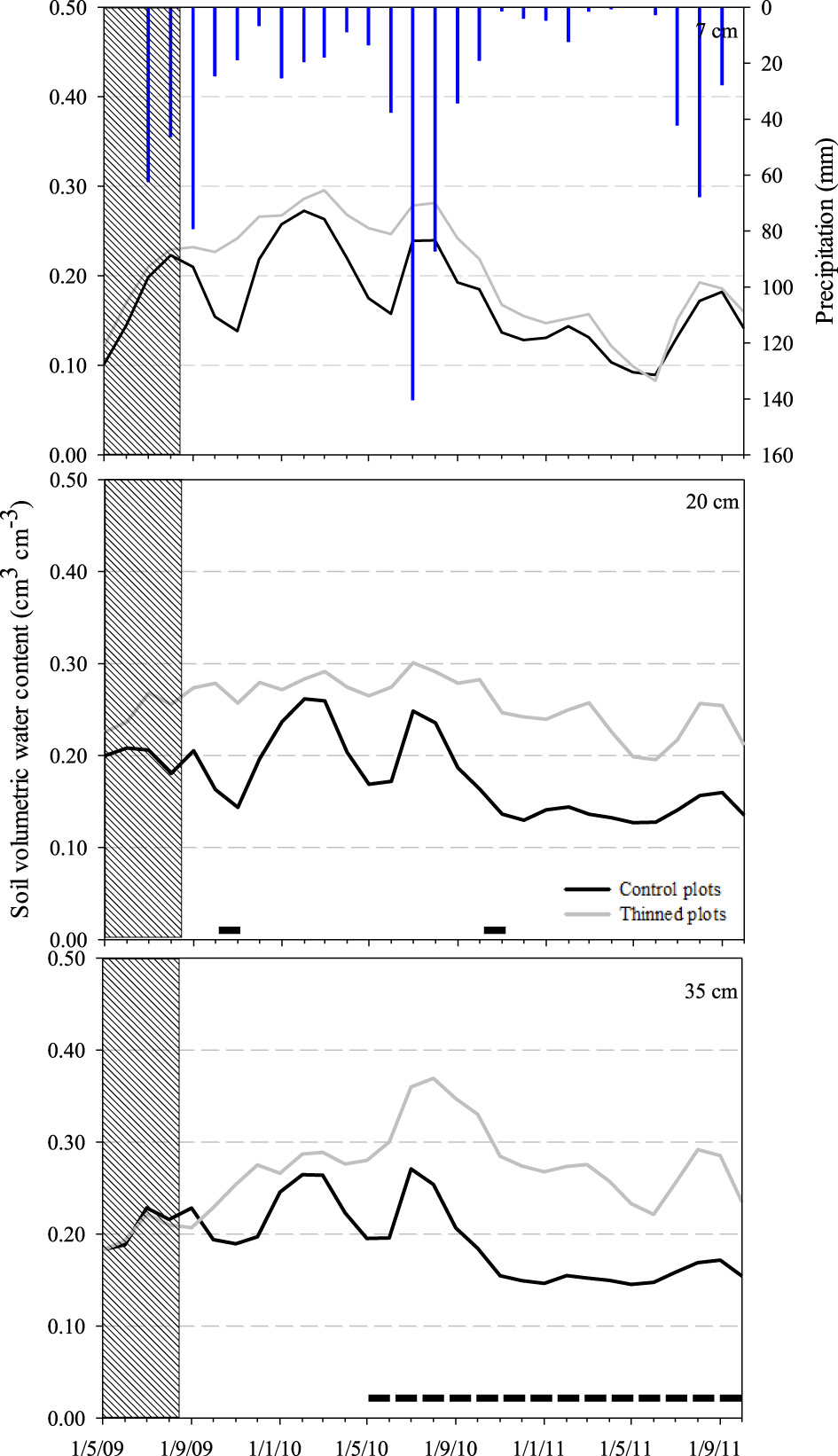
Monthly average soil volumetric water content measured at three different depths in both control and thinned plots. The black bold minus symbol represents the statistical significance between control and thinned plots. The vertical rectangle (hatched area) depicts the pre-treatment season and the vertical blue bars represent the precipitation.
At 20 cm depth, the thinned plots had a 0.12 ± 0.05 cm3 cm−3 higher than the control plots in October 2009 and 2010 (fall dry season). The significance of this difference was model-dependent (Figure 6). In control plots, the field capacity (0.26 cm3 cm−3) was attained in February and March 2010. In contrast, the low precipitation registered from October 2010 through October 2011 led the soil to the wilting point (0.10 cm3 cm−3) (Figure 6). On the other hand, thinned plots had a θ in the range of 0.20 to 0.30 cm3 cm−3. Although the wilting point and field capacity were at 0.13 and 0.45 cm3 cm−3, respectively, the θ was at the midpoint for the study period.
At 35 cm depth, the thinned plots had a consistently higher θ than the control plots, starting from May 2010 (spring dry season) through October 2011 (fall dry season) (Figure 6). The snowmelt of 2010 led to similar soil volumetric water content in thinned plots, throughout the soil profile (i.e., three different depths). After the dry season of 2010 (May), the precipitation of 140 mm (July) contributed to replenishing the soil (i.e., close to the field capacity of 0.41 cm3 cm−3), followed by a steady decrease until October 2011. Conversely, control plots had a low soil volumetric water content at 35 cm depth that followed a narrow range through the study period, likely attributed to tree root uptake.
3.5 Shallow soil water hydraulic gradients
In control plots, the total hydraulic head data showed depth-specific patterns (Figure 7A). During the study period, at all depths, the total head increased as a response to low precipitation events. At 7 cm depth, the total head was the most influenced by precipitation and dry spells, even reaching −1,200 cm in June 2011, while at 20 and 35 cm depths reached −700 and −800 cm, respectively.
Figure 7
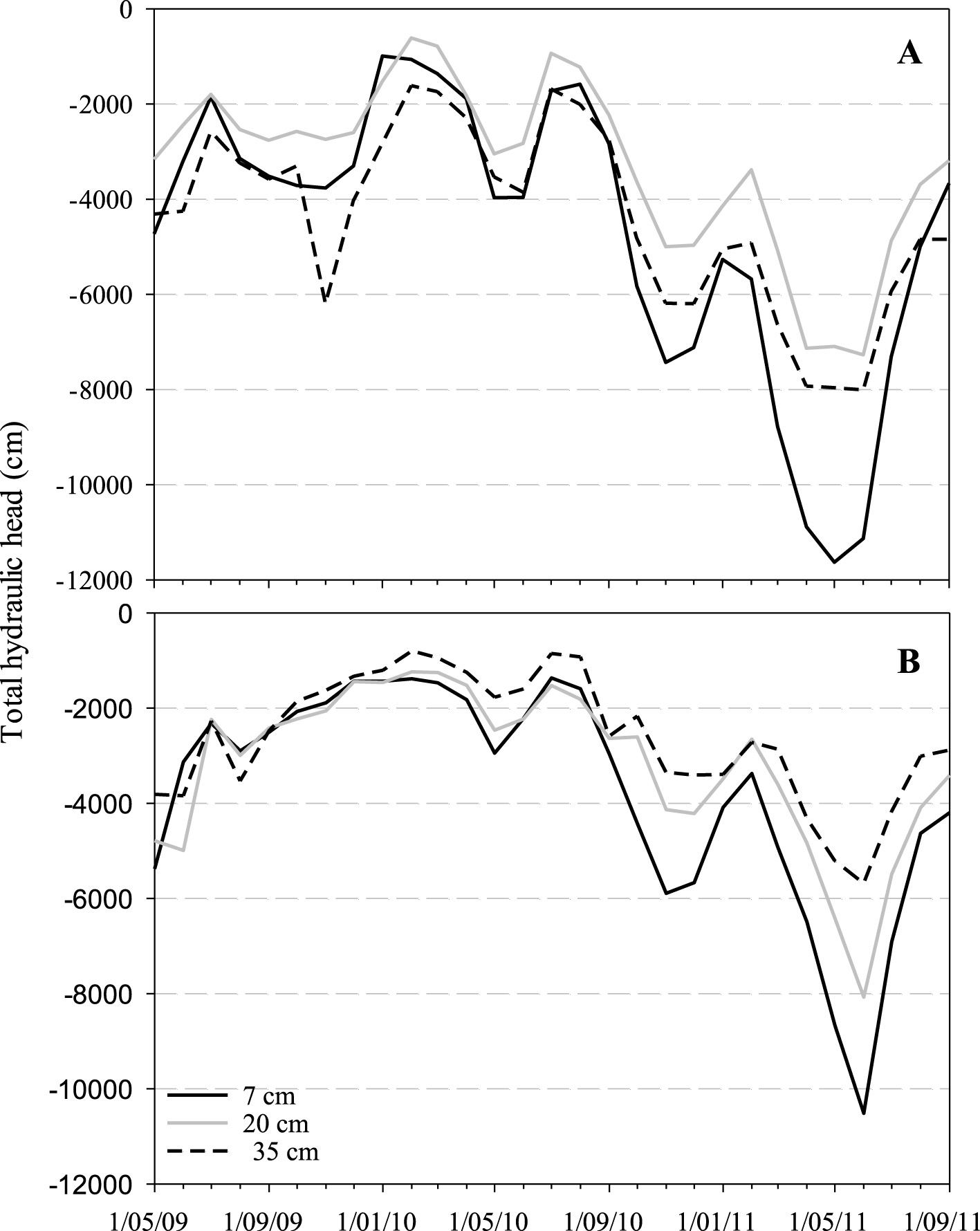
Monthly total hydraulic head (cm) across depths in control plots (A) and thinned plots (B).
In thinned plots, water flowed from the deeper layer (35 cm) to the shallower layer (7 cm) (Figure 7B). After the thinning treatment, all depths diminished in total head until September 2010. After this period, it increased (more negative), although at 35 cm depth, there was a less pronounced increase. Thus, at 35 cm depth, the total hydraulic head was in a range of −200 to −590 cm even with prolonged low precipitation (February and August 2011). The response and direction of water flow occurred after the thinning treatment, mainly due to the lack of tree influence, which likely diminished water uptake at deeper soil layers, thereby altering the total hydraulic head.
In control plots, during the study period, the hydraulic gradient was mainly positive at 7–20 cm depth with a sharp increase from January 2010 through December 2010. At this depth, the hydraulic gradient showed multiple peaks and fluctuations, mainly after precipitation (Figure 8A). At 20–35 cm depth, the hydraulic gradient was mostly negative. At this depth, the hydraulic gradient remained steady around zero, indicating minimal variation. The opposite direction at both depths was mainly due to water uptake by trees (probes were installed between three pines). The total hydraulic head corroborates the direction of water flow shown on the hydraulic gradients during low precipitation (April through July 2011).
Figure 8
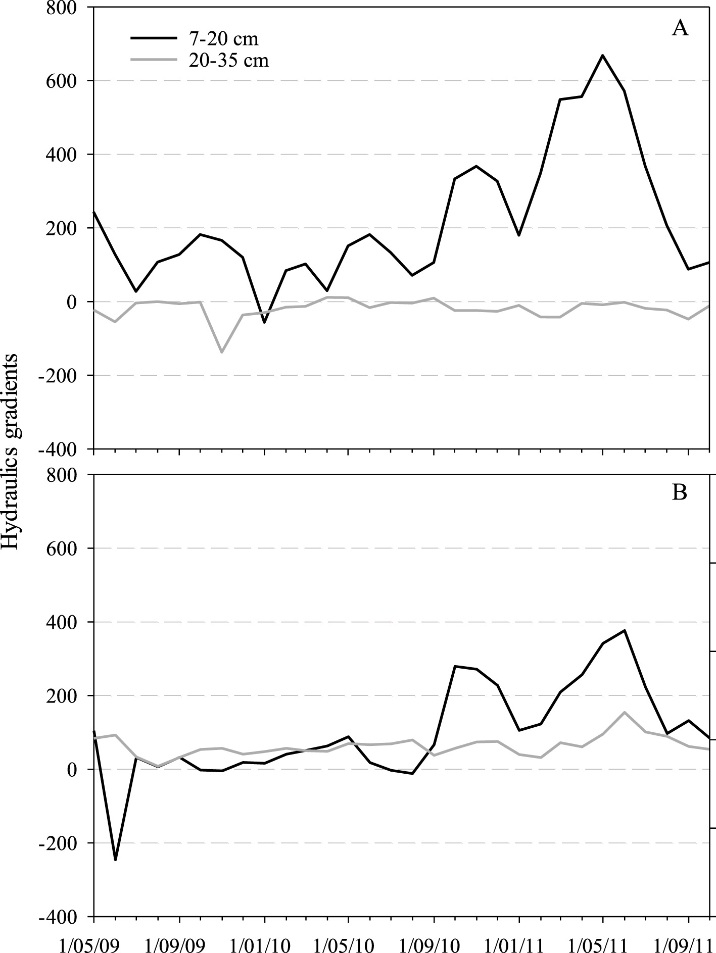
Monthly hydraulic gradients at two depths in control (A) and thinned plots (B).
In thinned plots, after the thinning treatment, the hydraulic gradient was positive at both depths (7–20 cm and 20–35 cm) even during low precipitation (February through June 2010 and from October 2010 to the first week of July 2011) (Figure 8B). At 7–20 cm depth, the hydraulic gradient increased steadily from October 2009 through May 2010. Henceforward, the hydraulic gradient had a sharp decrease until August 2011. At 20–35 cm depth, it remained relatively stable with small variation. During the described period, at both depths, water flow was from the high total head to the low total head as confirmed by the hydraulic head results (Figure 7B).
3.6 Shallow soil water flux quantification
Following thinning, at 7 to 20 cm depth, seasonal estimates of soil water flux in control plots ranged from −0.002 (dry season 2009) to 0.014 mm day−1 (snowmelt 2011), while for thinned plots, the mean q ranged from−0.060 (pre-treatment) to 0.051 mm day−1 (dry season 2011). Both plots showed similar trends in q with upward (+) and downward (–) directions, although the control plots showed slight upward and downward q movement (Figure 9A). The pre-treatment period showed a downward direction for both plots (i.e., control and thinned); none of these differences were significant (Table 4).
Figure 9
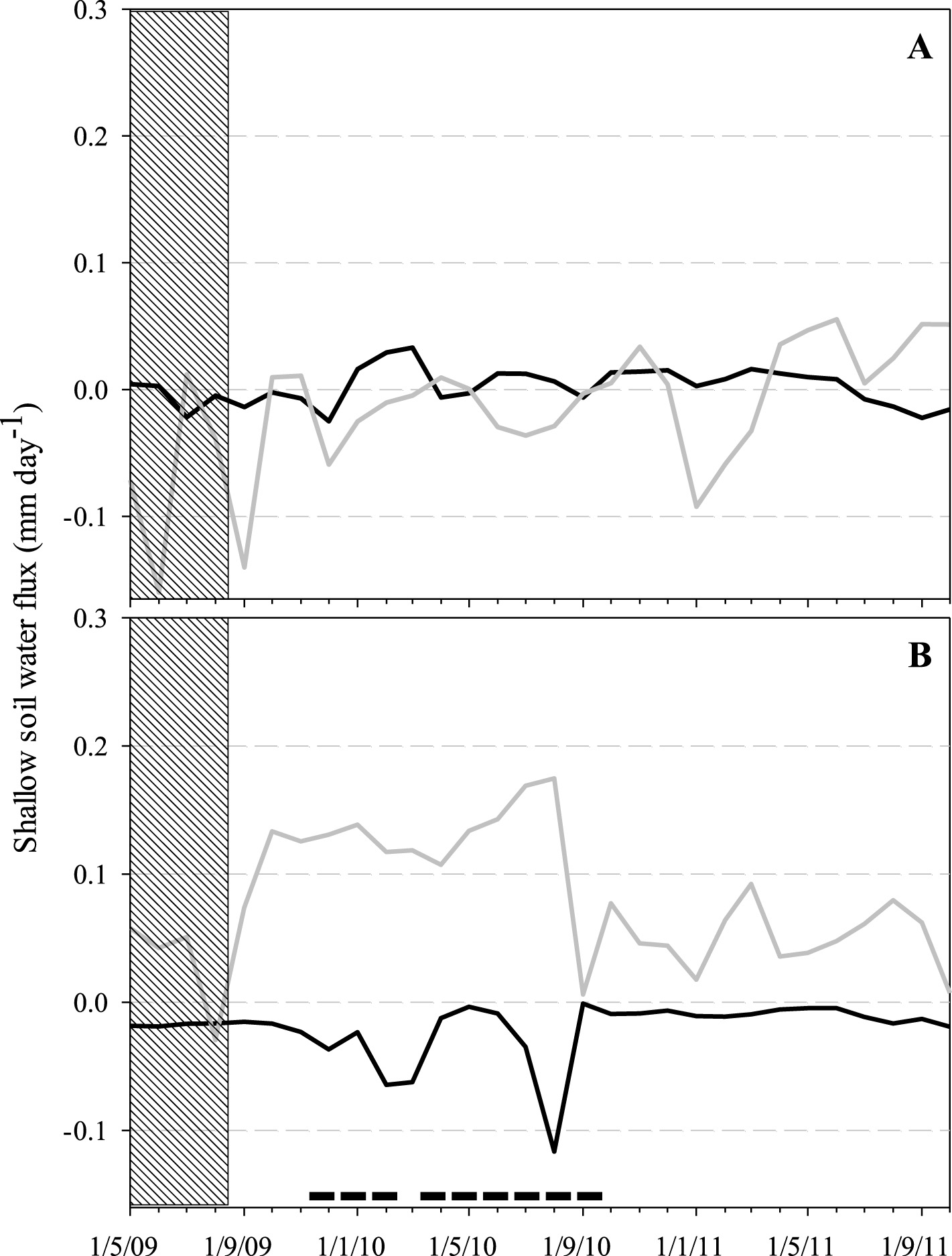
Shallow soil water flux at 7-20 cm depth (A) and 20-35 cm depth (B). The solid black and gray lines represent control and thinned plots, respectively. The bold black minus symbol depicts statistical significance. The vertical rectangle (hatched area) depicts the pre-treatment season.
Table 4
| 7–20 cm depth | 20–35 cm depth | |||||
|---|---|---|---|---|---|---|
| Season † | Control (SE) | Thinned (SE) | P -value | Control (SE) | Thinned (SE) | P -value |
| Pre-treatment | −0.005 (0.023) | −0.065(0.058) | 0.347 | −0.018 (0.029) | 0.030 (0.056) | 0.449 |
| Dry 2009 | −0.002 (0.028) | 0.010 (0.071) | 0.878 | −0.017 (0.039) | 0.133 (0.075) | 0.070 |
| Snow 2009–2010 | −0.005 (0.023) | −0.024 (0.057) | 0.757 | −0.028 (0.030) | 0.132 (0.058) | 0.019* |
| Snowmelt 2010 | 0.013 (0.018) | 0.002 (0.046) | 0.827 | −0.037 (0.028) | 0.113 (0.048) | 0.012* |
| Dry 2010 | −0.003 (0.020) | 0.001 (0.051) | 0.950 | −0.004 (0.032) | 0.134 (0.054) | 0.031* |
| Rainy 2010 | 0.006 (0.016) | −0.024 (0.042) | 0.498 | −0.040 (0.026) | 0.123 (0.041) | 0.005* |
| Dry 2010 | 0.013 (0.020) | 0.005 (0.051) | 0.879 | −0.009 (0.032) | 0.077 (0.054) | 0.163 |
| Snow 2010–2011 | 0.011 (0.017) | −0.018 (0.043) | 0.540 | −0.009 (0.027) | 0.036 (0.044) | 0.392 |
| Snowmelt 2011 | 0.014 (0.018) | 0.002 (0.046) | 0.798 | −0.007 (0.028) | 0.064 (0.048) | 0.202 |
| Dry 2011 | 0.010 (0.020) | 0.047 (0.051) | 0.500 | −0.004 (0.032) | 0.039 (0.054) | 0.481 |
| Rainy 2011 | −0.009 (0.016) | 0.034 (0.041) | 0.339 | −0.011 (0.026) | 0.063 (0.041) | 0.147 |
| Dry 2011 | −0.016 (0.022) | 0.051 (0.051) | 0.232 | −0.019 (0.034) | 0.007 (0.054) | 0.672 |
Shallow soil water flux (mm day−1) at two depths.
†Pre-treatment season (May-August 2009), (2) Dry season fall (October) and spring (May), (3) Snow season (November–January), (4) Snowmelt season (March-April), and (5) Rainy season season (June–September).
The asterisk depicts statistical significance between control and thinned plots at a depth of 20–35 cm.
Following thinning, at 20 to 35 cm depth, control plots differed significantly from thinned plots beginning with the snow season 2009–2010 (November 2009–January 2010) through the rainy season 2010 (June–September 2010; Figure 9B). During this period, in control plots, q was in downward direction with the lowest q of −0.040 ± 0.026 mm day−1 during the rainy season 2010 (June–September). In thinned plots, q was predominantly in upward direction with the highest q of 0.134 ± 0.054 mm day−1 during the dry season in May 2010 (Table 4).
4 Discussion
The effect of thinning observed in the soil volumetric water content after 8 months was mainly at 35 cm depth, and in the soil water flux after 3 months at the soil profile of 20 to 35 cm depth. There were no differences in the pre-treatment between forest stands, likely due to similar forest conditions (e.g., slope gradient, tree density, soil texture, and soil depth) before the thinning treatment carried out in mid-August 2009. Our findings revealed the shallow soil water dynamics in response to different seasons and highlight the critical role of post-thinning.
4.1 Soil volumetric water content
Our results suggest that thinning increases soil volumetric water content at 35 cm depth, likely stored at the bottom of the soil column on a rock surface. Following the thinning treatment, the difference in soil volumetric water content between control and thinned plots increased from May 2010 through October 2011, driven by changes in forest structure. Thinning reduced the canopy cover and tree density, leaving open spaces covered by scattered slash. These changes aimed to maintain higher soil volumetric water content for longer periods compared to control plots, even during the lowest precipitation recorded (i.e., the rainy season) in 2011 (Figure 6). The weathered bedrock vadose zone, referred to as “rock moisture” (Hahm et al., 2022; Luo et al., 2024), mitigates drought impacts by storing water in wet years and releasing it in dry periods (Callahan et al., 2022). Forest structure is a key factor influencing soil moisture at the upper 50 cm depth, especially during drought periods (Belmonte et al., 2022). Thinning creates forest gaps, enhancing soil moisture through three key processes: (1) reduced canopy interception (Wang et al., 2015), (2) reduced water uptake (Marthews et al., 2008), and (3) lower transpiration rates (Ritter et al., 2005). Our results agree with Lucas-Borja et al. (2018), who reported warmer soil surface temperature and higher soil volumetric water content in straw mulch plots compared to control plots in a Mediterranean forest. Similar to our study, thinning a semi-arid ponderosa forest increased soil moisture in the first 100 cm vs. unthinned forests (Sankey and Tatum, 2022). Another study reported temporal effects on soil moisture response in thinned stands. The onset of soil moisture depletion was delayed in thinned vs. control stands. However, in years with above-average precipitation, thinned and control stands reached their maximum water storage capacity (Hardage et al., 2022).
4.2 Shallow soil water flux
Our results revealed a more nuanced effect of forest thinning on soil water flux than initially hypothesized. Specifically, the hypothesis, “In treated plots, water flows in downward direction during the snowmelt and rainy season,” was partially confirmed. It was not supported during the snowmelt period (upward water flow), but was supported during the rainfall period in 2010 (downward water flow).
During the snowmelt season (2010), differences in soil and slash cover temperatures influenced the upward water flux. This was confirmed by the hydraulic head gradients, with a higher water potential at 35 cm and a lower water potential at 7 cm depth. The differences in gradients were likely influenced by high evaporative demand at the surface. In thinned plots, solar radiation reached the slash cover directly, increasing the soil temperature and slash cover, which provided the latent energy for evaporation (Heck et al., 2020). Concurrently, wind removed water vapor from the surface, sustaining a high vapor pressure deficit (Davarzani et al., 2014). Both variables influenced the upward flow observed during this period. Soil temperature gradients influence soil water flux in unsaturated soils; however, the magnitude of the temperature effect depends on the volumetric water content (Bach, 1992). Gierke et al. (2016) characterized the snowmelt in the same watershed as slow, uniform infiltration that primarily fills soil micropores, creating a tightly-bound water source for water uptake during the dry spring. The upward flux we reported was a key mechanism for redistributing moisture in the shallow root zone, although the majority of the snowmelt water likely infiltrated and was stored at the weathered bedrock. Contrary to our results and a different setup, Iwata et al. (2010) reported downward water flux as the snow melted in above-zero temperatures in an agricultural field devoid of vegetation.
During the rainy season (2010), we observed a complex pattern of water flux. It was downward from 7 to 20 cm and upward from 35 to 20 cm. This pattern likely occurred due to the water uptake by pine seedlings known as hydraulic redistribution. This process occurs when water moves from deeper soil layers (moist soil) upward to shallow soil layers (drier soil) through the root system, usually during the night when transpiration has diminished (Richards and Caldwell, 1987; Brooks et al., 2002). This is a plausible process on our site, where ponderosa pine seedlings can extract water from shallow, rocky soils (Rose et al., 1997) despite root growth being influenced by soil moisture and bulk density (Siegel-Issem et al., 2005). According to the tree density assessment conducted in March 2010, pine seedlings averaged 163 per ha in thinned plots and 128 per ha in control plots. Fornwalt et al. (2017) reported similar total understory plant cover on mulching plots (i.e., similar to our treatment) vs. control plots after 2–4 years of the treatment in a mixed conifer forest. Warren et al. (2011) reported that root water extraction was mainly in the upper soil horizon (20 cm) in old-growth ponderosa pine. Isotope analysis from the same watershed showed that trees take water from shallow and deep layers during the rainy season (Gierke et al., 2016). Their results detailed a seasonal pattern where trees relied exclusively on the shallow water pool during the dry spring, then shifted to a mixture of both shallow and deep water sources during the monsoon, and continued to access the deeper water for months after the rains ended.
Our hypothesis, “During the low water input (dry season), treated plots may have upward water flux,” was confirmed. The upward water flux likely resulted from a high evaporative demand (similar to the observed snowmelt season), which created a hydraulic gradient that moved water upward from storage at the base of the rock column. This process reflected water redistribution from the weathered bedrock interface toward a drier surface layer. The upward water flux was observed right after the thinning treatment from October 2009 (dry season) through the end of the study (October 2011), with noticeable differences in the hydraulic gradients in the shallow soil matrix. The scattered slash covered the topsoil and kept the soil warmer compared to the soil under the canopy in control plots. The slash absorbed and re-radiated solar radiation throughout the year, creating a warmer microclimate at the soil surface. This increase in temperature likely enhanced water loss via evaporation. Solar radiation has been widely studied, resulting in warmer soil temperatures in treated than in control plots due to the lack of canopy cover (Everett and Sharrow, 1985; Breshears et al., 1998; Tang et al., 2005; Moroni et al., 2009; Garduño et al., 2010). In addition, forest floor residues (e.g., slash) have been shown to influence soil temperature patterns (Liechty et al., 1992; Zabowski et al., 2000). Similar to our results but different thinning setup, Sun et al. (2016) reported increased soil evaporation after strip thinning in a Japanese cypress forest. They reported that radiation was highly correlated, followed by vapor pressure deficit during this process. Tatum et al. (2025) measured the soil water potential in a thinned Ponderosa forest. The vertical gradient in soil water potential observed in the thinned treatment suggests upward water movement from deep soil layers (less negative at 100 cm) to the shallow root zone (more negative at 25 cm) during the dry season.
4.3 Study limitations
The interpretation of our findings on soil water dynamics should be considered within the inherent context of hydrological data uncertainty. Hydrological data are subject to multiple sources of uncertainty, with typical magnitudes of 10 to 40% (McMillan et al., 2018). First, the Darcy-Richards equation relies on key assumptions: (1) water flow is essentially one-dimensional in the vertical direction, (2) the soil is isotropic with uniform hydraulic properties horizontally, and (3) steady-state conditions are approximated over the measurement interval (Warrick, 2003). This approach offers a reliable estimate of shallow soil water fluxes, even though natural soil systems may differ from these ideal circumstances, introducing potential error.
Second, our study considered the uncertainty associated with the scale-up process (using a limited number of experimental blocks, n = 4). Although this design is common in large-scale experiments, it introduces uncertainty when extrapolating results across broader and heterogeneous landscapes. The statistically significant treatment effects observed in soil volumetric content and shallow soil water flux were detectable across this underlying uncertainty and represented a relevant hydrological response to thinning.
4.4 Management implications
The hydrological response to thinning observed in our study is specific to the conditions of a mixed conifer forest overlying fractured limestone bedrock. The direct application of our findings is most relevant to forest and water managers operating in similar climate and shallow, rocky soil environments. Our findings provide critical-grounded guidance for managers aiming to enhance forest resilience and water storage during drought. Despite an increase in soil water storage, thinning had nuanced effects on water flux, mainly in upward direction. This process translates into more stored water and less water lost via evaporation under soils with scattered slash. For managers, this implies that strategic thinning can be a proactive strategy to mitigate drought stress in conifer forests. By reducing stand density, managers can effectively delay the onset of soil water deficit, thereby reducing tree mortality and susceptibility to pests, which are often exacerbated by drought.
5 Conclusions
Our study demonstrates that thinning mixed conifer forest stands on fracture limestone led to soil volumetric water content storage, likely due to water accumulation in the weathered bedrock vadose zone, which subsequently contributed to upward water flux during dry periods.
These findings provide valuable insights for water managers seeking to make informed land management decisions that support sustainable water use and ecosystem health. By considering the impact of forest thinning on soil water dynamics, managers can promote healthy forest ecosystems while addressing climate change-related concerns. It is important to include thinning practices to keep trees and seedlings at low density to avoid water loss by evapotranspiration by contributing to groundwater recharge, especially in regions facing increasing water scarcity due to climate change.
Further research is necessary to understand the long-term effects of thinning on the hydrological processes of forest ecosystems under changing climatic conditions. Such studies should consider the effects of thinning intensity and techniques on forest hydrology to develop optimal thinning practices for different forest types and climatic conditions. By integrating climate change considerations into forest management strategies, water managers can enhance the resilience of forest ecosystems and ensure sustainable water resources.
Statements
Data availability statement
The soil volumetric water content, soil matric potential, and soil temperature data generated in this study have been deposited in the Zenodo repository under DOI: 10.5281/zenodo.17297044.
Author contributions
HG: Conceptualization, Investigation, Methodology, Project administration, Writing – original draft, Writing – review & editing. AF: Conceptualization, Funding acquisition, Resources, Writing – review & editing. BN: Funding acquisition, Resources, Writing – review & editing. DV: Formal analysis, Writing – review & editing. MS: Resources, Writing – review & editing.
Funding
The author(s) declare that financial support was received for the research and/or publication of this article. This study was partially funded by the Sacramento Mountains Hydrogeology Study of the New Mexico Bureau of Geology and Mineral Resources, the New Mexico Agricultural Experimental Station, the NSF-NM EPSCoR UROP program, and Hatch/NIFA #1015539.
Acknowledgments
Special thanks to Ricardo Martinez and Angel Morales for providing the logistical support to carry out this project. We also want to acknowledge the field data collection help provided by undergraduate students from New Mexico State University and New Mexico Tech.
Conflict of interest
The authors declare that the research was conducted in the absence of any commercial or financial relationships that could be construed as a potential conflict of interest.
Generative AI statement
The author(s) declare that no Gen AI was used in the creation of this manuscript.
Any alternative text (alt text) provided alongside figures in this article has been generated by Frontiers with the support of artificial intelligence and reasonable efforts have been made to ensure accuracy, including review by the authors wherever possible. If you identify any issues, please contact us.
Publisher’s note
All claims expressed in this article are solely those of the authors and do not necessarily represent those of their affiliated organizations, or those of the publisher, the editors and the reviewers. Any product that may be evaluated in this article, or claim that may be made by its manufacturer, is not guaranteed or endorsed by the publisher.
Supplementary material
The Supplementary Material for this article can be found online at: https://www.frontiersin.org/articles/10.3389/ffgc.2025.1648254/full#supplementary-material
References
1
Atalar F. Beyazoglu O. Fernald A. G. Burney O. T. VanLeeuwen D. M. Cram D. S. et al . (2021). A case study of runoff and sediment yield in areas subjected to different forest thinning operations in a northern New Mexico forest. JSWC76, 293–302. doi: 10.2489/jswc.2021.00135
2
Bach L. B. (1992). Soil water movement in response to temperature gradients: experimental measurements and model evaluation. SSSAJ56, 37–46. doi: 10.2136/sssaj1992.03615995005600010005x
3
Bai S. H. Dempsey R. Reverchon F. Blumfield T. J. Ryan S. Cernusak L. A. et al . (2017). Effects of forest thinning on soil-plant carbon and nitrogen dynamics. Plant Soil411, 437–449. doi: 10.1007/s11104-016-3052-5
4
Belmonte A. Sankey T. T. Biederman J. Bradford J. B. Kolb T. (2022). Soil moisture response to seasonal drought conditions and post-thinning forest structure. Ecohydrology15:e2406. doi: 10.1002/eco.2406
5
Bond W. (1998). Soil Physical Methods for Estimating Discharge: Basics of Recharge and Discharge Part 3. Collongwood: CSIRO Publishing. doi: 10.1071/9780643105355
6
Breshears D. D. Nyhan J. W. Heil C. E. Wilcox B. P. (1998). Effects of woody plants on microclimate in a semiarid woodland: soil temperature and evaporation in canopy and intercanopy patches. J. Plant Sci.159, 1010–1017. doi: 10.1086/314083
7
Brooks J. R. Meinzer F. C. Coulombe R. O. Gregg J. (2002). Hydraulic redistribution of soil water during summer drought in two contrasting Pacific Northwest coniferous forests. Tree Physiol.22, 1107–1117. doi: 10.1093/treephys/22.15-16.1107
8
Callahan R. P. Riebe C. S. Sklar L. S. Pasquet S. Ferrier K. L. Hahm W. J. et al . (2022). Forest vulnerability to drought controlled by bedrock composition. Nat. Geosci.15, 714–719. doi: 10.1038/s41561-022-01012-2
9
Campbell Scientific L. T. D. (2006). 229 Heat Dissipation Matric Water Potential Sensor: Instruction Manual. Campbell Scientific Ltd: Loughborough, UK.
10
Campbell G. (2008). Modeling available soil moisture. Dec. Dev. Support Appl.1–4.
11
Cobos D. R. Chambers C. (2009). Calibrating ECH2O Soil Moisture Sensors. Application Note. Pullman WA: Decagon Devices.
12
Cook B. Ault T. R. Smerdon J. E. (2015). Unprecedented 21st century drought risk in the American southwest and central Plains. Sci. Adv. 1:82. doi: 10.1126/sciadv.1400082
13
Courcot B. Lemire D. Bélanger N. (2024). Dynamics of soil water potential as a function of stand types in a temperate forest: emphasis on flash droughts. Geodermal Reg.38:e00850. doi: 10.1016/j.geodrs.2024.e00850
14
Cram D. S. Baker T. T. Fernald A. G. Madrid A. Rummer B. (2007). Mechanical thinning impacts on runoff, infiltration, and sediment yield following fuel reduction treatments in a southwestern dry mixed conifer forest. JSWC62, 359–366. doi: 10.1080/00224561.2007.12435984
15
Davarzani H. Smits K. Tolene R. M. Illangasekare T. (2014). Study of the effect of wind speed on evaporation from soil through integrated modeling of the atmospheric boundary layer and shallow subsurface. Water Resour. Res.50, 661–680. doi: 10.1002/2013WR013952
16
Decagon Devices (2008). ECHO2-EC-TM: Water Content, EC, and Temperature Sensors. Operator's Manual. Version 5. Pullman WA: Decagon Devices.
17
del Campo A. D. Otsuki K. Serengil Y. Blanco J. A. Yousefpour R. Wei X. (2022). A global synthesis on the effects of thinning on hydrological processes: implications for forest management. For. Ecol. Manag.519:120324. doi: 10.1016/j.foreco.2022.120324
18
Di Prima S. Bagarello V. Angulo-Jaramillo R. Bautista I. Cerdai A. Del Campo A. et al . (2017). Impacts of thinning of a Mediterranean oak forest on soil properties influencing water infiltration. J. Hydrol. Hydromech65, 276–286. doi: 10.1515/johh-2017-0016
19
Dingman S. L. (2008). Physical Hydrology, 2nd edn. Illinois: Waveland Press Inc., 646.
20
Domenico P. A. Schwartz F. W. (1997). Physical and Chemical Hydrogeology, 2nd edn. New York: John Wiley & Sons Inc., 506.
21
Everett R. L. Sharrow S. H. (1985). Soil water and temperature in harvested and non-harvested pinyon-juniper stands. Intermountain Res. Station342, 1–5.
22
Flury M. Wai N. N. (2003). Dyes as tracers for vadose zone hydrology. Rev. Geophys. 41, 1–37. doi: 10.1029/2001RG000109
23
Fornwalt P. J. Rocca M. E. Battaglia M. A. Rhoades C. C. Ryan M. G. (2017). Mulching fuels treatments promote understory plant communities in three Colorado, USA, coniferous forest types. For. Ecol. Manag.385, 214–224. doi: 10.1016/j.foreco.2016.11.047
24
Fulé P. Z. Korb J. E. Wu R. (2009). Changes in forest structure of a mixed conifer forest, southwestern Colorado, USA. For. Ecol. Manag.258, 1200–1210. doi: 10.1016/j.foreco.2009.06.015
25
Gardner W. R. (1958). Some steady-state solutions of the unsaturated moisture flow equation with application to evaporation from a water table. Soil Sci.85, 228–232. doi: 10.1097/00010694-195804000-00006
26
Garduño H. R. Fernald A. VanLeeuwen D. (2015). Non-commercial thinning effects on runoff and sediment yield in mixed conifer New Mexico forest. JSWC70, 12–22. doi: 10.2489/jswc.70.1.12
27
Garduño H. R. Fernald A. G. Cibils A. F. VanLeeuwen D. M. (2010). Response of understory vegetation and soil moisture to infrequent heavy defoliation of chemically thinned juniper woodland. J. Arid Environ. 74, 291–297. doi: 10.1016/j.jaridenv.2009.08.005
28
Gierke C. Newton B. T. Phillips F. M. (2016). Soil-water dynamics and tree water uptake in the Sacramento Mountains of New Mexico (USA): a stable isotope study. Hydrogeol J. 24:805. doi: 10.1007/s10040-016-1403-1
29
Hahm W. J. Dralle D. N. Sanders M. Bryk A. B. Fauria K. E. Huang M. H. et al . (2022). Bedrock vadose zone storage dynamics under extreme drought: consequences for plant water availability, recharge, and runoff. Water Resour. Res.58:e2021WR031781. doi: 10.1029/2021WR031781
30
Hanks R. J. (1992). Applied Soil Physics: Soil Water and Temperature Applications, 2nd edn. New York, NY: Springer-Verlag, 159. doi: 10.1007/978-1-4612-2938-4_5
31
Hardage K. Wheelock S. J. Gaffney R. O'Halloran T. Serpa B. Grant G. et al . (2022). Soil moisture and micrometeorological differences across reference and thinned stands during extremes of precipitation, southern Cascade Range. Front. For. Glob. Change5:898998. doi: 10.3389/ffgc.2022.898998
32
Harr R. D. (1977). Water flux in soil and subsoil on a steep forested slope. J. Hydrol. 33, 37–58. doi: 10.1016/0022-1694(77)90097-X
33
Heck K. Coltman E. Schneider J. Helmig R. (2020). Influence of radiation on evaporation rates: a numerical analysis. Water Resour. Res.56:e2020WR027332. doi: 10.1029/2020WR027332
34
Iwata Y. Hirota T. Hayashi M. Suzuki S. Hasegawa S. (2010). Effects of frozen soil and snow cover on cold-season soil water dynamics in Tokachi, Japan. Hydrol. Process24, 1735–1765. doi: 10.1002/hyp.7621
35
Kupers S. J. Engelbrecht B. M. Hernández A. Wright S. J. Wirth C. Rüger N. et al . (2019a). Growth responses to soil water potential indirectly shape local species distributions of tropical forest seedlings. J. Ecol.107, 860–874. doi: 10.1111/1365-2745.13096
36
Kupers S. J. Wirth C. Engelbrecht B. M. Rüger N. (2019b). Dry season soil water potential maps of a 50 hectare tropical forest plot on Barro Colorado Island, Panama. Sci. Data6:63. doi: 10.1038/s41597-019-0072-z
37
Lal R. Shukla M. K. (2004). Principles of Soil Physics, 1st edn. New York: Marcel Dekker Inc., 716. doi: 10.4324/9780203021231
38
Lee R. (1980). Forest Hydrology, 1st edn. New York: Columbia University Press, 349. doi: 10.7312/lee-91170
39
Liechty H. O. Holmes M. J. Reed D. D. Mroz G. D. (1992). Changes in microclimates after stand conversion in two northern hardwood stands. For. Ecol. Manag.50, 253–264. doi: 10.1016/0378-1127(92)90340-F
40
Liu X. Chen X. Zhang Z. Liu W. Peng T. McDonnell J. J. et al . (2025). The role of rock fractures on tree water use of water stored in bedrock: mixing and residence times. EGUsphere2025, 1–43. doi: 10.5194/egusphere-2025-3937
41
Löffler J. (2007). The influence of micro-climate, snow cover, and soil moisture on ecosystem functioning in high mountains. J. Geogr. Sci. 17, 3–19. doi: 10.1007/s11442-007-0003-3
42
Lucas-Borja M. E. Zema D. A. Carrà B. G. Cerdà A. Plaza-Alvarez P. A. Cózar J. S. et al . (2018). Short-term changes in infiltration between straw mulched and non-mulched soils after wildfire in Mediterranean forest ecosystems. Ecol. Eng.122, 27–31. doi: 10.1016/j.ecoleng.2018.07.018
43
Luo Z. Fan J. Shao M. A. Yang Q. Li M. (2024). Rock moisture reinforces belowground water storage under different precipitation scenarios and vegetation coverage. J. Hydrol.636:131276. doi: 10.1016/j.jhydrol.2024.131276
44
Madrid A. Fernald A. G. Baker T. T. VanLeeuwen D. M. (2006). Evaluation of silvicultural treatment effects on infiltration, runoff, sediment yield, and soil moisture in a mixed conifer New Mexico forest. JSWC61, 159–168. doi: 10.1080/00224561.2006.12435876
45
Maloney E. D. Camargo S. J. Chang E. Colle B. Fu R. Geil K. L. et al . (2014). North American climate in CMIP5 experiments: part III: assessment of twenty-first-century projections. J. Clim.27, 2230–2270. doi: 10.1175/JCLI-D-13-00273.1
46
Marthews T. R. Burslem D. F. R. P. Paton S. R. Yangüez F. Mullins C. E. (2008). Soil drying in a tropical forest: three distinct environments controlled by gap size. Ecol. Modell.216, 369–384. doi: 10.1016/j.ecolmodel.2008.05.011
47
McGuire K. J. Likens G. E. (2011). “Historical roots of forest hydrology and biogeochemistry,” in Forest Hydrology and Biogeochemistry: Synthesis of Past Research and Future Directions, Vol. 1, eds. D. F. Levia, D. Carlyle-Moses, T. Tanaka (Netherlands: Springer), 3–26. doi: 10.1007/978-94-007-1363-5_1
48
McMillan H. K. Westerberg I. K. Krueger T. (2018). Hydrological data uncertainty and its implications. Wiley Interdiscip. Rev. Water5:e1319. doi: 10.1002/wat2.1319
49
Moroni M. T. Carter P. Q. Ryan D. A. (2009). Harvesting and slash piling affects soil respiration, soil temperature, and soil moisture regimes in Newfoundland boreal forests. Can. J. Soil Sci.89, 343–355. doi: 10.4141/CJSS08027
50
Newton T. Mammer E. Re Velle P. Garduño H. (2015). Sacramento Mountains Watershed Study - The Effects of Three Thinning on the Local Hydrologic System. New Mexico Bureau of Geology and Mineral Resources Open-File Report. doi: 10.58799/OFR-576
51
Novick K. A. Ficklin D. L. Baldocchi D. Davis K. J. Ghezzehei T. A. Konings A. G. et al . (2022). Confronting the water potential information gap. Nat. Geosci15, 158–164. doi: 10.1038/s41561-022-00909-2
52
Park J. Taekyu K. Minkyu M. Sungsik C. Daun R. Hyun S. K. et al . (2018). Effects of thinning intensities on tree water use, growth, and resultant water use efficiency of 50-year-old Pinus koraiensis forest over four years. For. Ecol. Manag. 408, 121–128. doi: 10.1016/j.foreco.2017.09.031
53
Richards J. H. Caldwell M. M. (1987). Hydraulic lift: substantial nocturnal water transport between soil layers by Artemisia tridentata roots. Oecologia73, 486–489. doi: 10.1007/BF00379405
54
Richards L. A. (1931). Capillary conduction of liquids through porous mediums. J. Appl. Phys.1, 318–333. doi: 10.1063/1.1745010
55
Ritter E. Dalsgaard L. Einhorn K. S. (2005). Light, temperature and soil moisture regimes following gap formation in a semi-natural beech-dominated forest in Denmark. For. Ecol. Manage.206, 15–33. doi: 10.1016/j.foreco.2004.08.011
56
Rose R. Haase D. L. Kroiher F. Sabin T. (1997). Root volume and growth of ponderosa pine and Douglas-fir seedlings: a summary of eight growing seasons. West. J. Appl. For.12, 69–73. doi: 10.1093/wjaf/12.3.69
57
Salve R. Rempe D. M. Dietrich W. E. (2012). Rain, rock moisture dynamics, and the rapid response of perched groundwater in weathered, fractured argillite underlying a steep hillslope. Water Resour. Res.48, 1–25. doi: 10.1029/2012WR012583
58
Sankey T. Tatum J. (2022). Thinning increases forest resiliency during unprecedented drought. Sci. Rep12:9041. doi: 10.1038/s41598-022-12982-z
59
Seager R. Ting M. Alexander P. Nakamura J. Liu H. Li C. et al . (2023). Oceanforcing of cool season precipitation drives ongoing and future decadal drought in southwestern North America. npj Clim. Atmos. Sci. 6:141. doi: 10.1038/s41612-023-00461-9
60
Siegel-Issem C. M. Burger J. A. Powers R. F. Ponder F. Patterson S. C. (2005). Seedling root growth as a function of soil density and water content. Soil Sci. Soc. Am. J.69, 215–226. doi: 10.2136/sssaj2005.0215
61
Sopper W. E. Lull H. W. (1967). “International symposium on forest hydrology,” in Proceedings of a National Science Foundation advanced Science Seminar Held at the Pennsylvania State University, University Park, Pennsylvania (Pergamon Press).
62
Sun X. Onda Y. Otsuki K. Kato H. Gomi T. (2016). The effect of strip thinning on forest floor evaporation in a Japanese cypress plantation. Agric. For. Meteorol.216, 48–57. doi: 10.1016/j.agrformet.2015.10.006
63
Tang J. M. Qi Y. Xu M. Misson L. Goldstein A. H. (2005). Forest thinning and soil respiration in a ponderosa pine plantation in the Sierra Nevada. Tree Physiol.25, 57–66. doi: 10.1093/treephys/25.1.57
64
Tatum J. Sankey T. T. Belmonte A. Dymond S. F. Woolley T. (2025). Five years of hourly soil water potential monitoring demonstrates forest thinning benefits in the North American Southwest. Ecohydrology18:e70104. doi: 10.1002/eco.70104
65
Thorne J. H. Choe H. Stine P. A. Chambers J. C. Holguin A. Kerr A. C. et al . (2018). Climate change vulnerability assessment of forests in the Southwest USA. Clim. Change148, 387–402. doi: 10.1007/s10584-017-2010-4
66
van Genuchten M. T. (1980). A closed-form equation for predicting the hydraulic conductivity of unsaturated soils. Soil Sci. Soc. Am. J44, 892–898. doi: 10.2136/sssaj1980.03615995004400050002x
67
van Genuchten M. T. Leij F. J. Yates S. R. (1991). The RETC Code for Quantifying the Hydraulic Functions of Unsaturated Soils. U.S. Department of Agriculture, Agricultural Research Service.
68
Wang T. Xu Q. Gao D. Zhang B. Zuo H. Jiang J. et al . (2021). Effects of thinning and understory removal on the soil water-holding capacity in Pinus massoniana plantations. Sci. Rep.11:13029. doi: 10.1038/s41598-021-92423-5
69
Wang Z. Bao W. Yan X. (2015). Non-structural carbohydrate levels of three co-occurring understory plants and their responses to forest thinning by gap creation in a dense pine plantation. J. For. Res.26, 391–396. doi: 10.1007/s11676-015-0073-5
70
Warren J. M. Brooks J. R. Dragila M. I. Meinzer F. C. (2011). In situ separation of root hydraulic redistribution of soil water from liquid and vapor transport. Oecologia166, 899–911. doi: 10.1007/s00442-011-1953-9
71
Warrick A. W. (2003). Soil Water Dynamics. New York, NY: Oxford University Press. doi: 10.1093/oso/9780195126051.001.0001
72
Weiler M. McDonnell J. J. (2004). “Water storage and movement,” in Encyclopedia of Forest Sciences, eds. J. Burley, J. Evans, J. A. Youngquist (Oxford: Elsevier), 1253–1260. doi: 10.1016/B0-12-145160-7/00249-0
73
Western Regional Climate Center (WRCC) (2024). Available online at: https://wrcc.dri.edu/cgi-bin/cliMAIN.pl?nm1931 (Accessed March 27, 2024).
74
Williams A. P. Cook B. I. Smerdon J. E. (2022). Rapid intensification of the emerging southwestern North American megadrought in 2020–2021. Nature Clim. 12, 232–234. doi: 10.1038/s41558-022-01290-z
75
Xu Q. Liu S. Wan X. Jiang C. Song X. Wang J. et al . (2012). Effects of rainfall on soil moisture and water movement in a subalpine dark coniferous forest in southwestern China. Hydrol. Process26, 3800–3809. doi: 10.1002/hyp.8400
76
Yang H. Choi H. T. Lim H. (2019). Effects of forest thinning on the long-term runoff changes of coniferous forest plantation. Water11:2301. doi: 10.3390/w11112301
77
Zabowski D. Java B. Scherer G. Everett R. L. Ottrnar R. (2000). Timber harvesting residue treatment: part 1. Responses of conifer seedlings, soils, and microclimate. For. Ecol. Manag126, 25–34. doi: 10.1016/S0378-1127(99)00081-X
78
Zhang F. Zhang C. (2021). Probing water partitioning in unsaturated weathered rock using nuclear magnetic resonance. Geophysics 86, WB131–WB147. doi: 10.1190/geo2020-0591.1
79
Zhang X. Guan D. Li W. Sun D. Jin C. Yuan F. et al . (2018). The effects of forest thinning on soil carbon stocks and dynamics: a meta-analysis. For. Ecol. Manag.429, 36–43. doi: 10.1016/j.foreco.2018.06.027
Summary
Keywords
weathered bedrock, percolation, soil moisture storage, matric potential, forest resiliency
Citation
Garduño HR, Fernald AG, Newton BT, VanLeeuwen DM and Shukla MK (2025) Hydrological response to thinning in forest stands: analysis of soil volumetric water content and soil water flux. Front. For. Glob. Change 8:1648254. doi: 10.3389/ffgc.2025.1648254
Received
16 June 2025
Accepted
27 October 2025
Published
28 November 2025
Volume
8 - 2025
Edited by
Fengjing Liu, Michigan Technological University, United States
Reviewed by
Jessica Young-Robertson, University of Alaska Fairbanks, United States
Ufuk Özkan, Izmir Katip Celebi University, Türkiye
Updates
Copyright
© 2025 Garduño, Fernald, Newton, VanLeeuwen and Shukla.
This is an open-access article distributed under the terms of the Creative Commons Attribution License (CC BY). The use, distribution or reproduction in other forums is permitted, provided the original author(s) and the copyright owner(s) are credited and that the original publication in this journal is cited, in accordance with accepted academic practice. No use, distribution or reproduction is permitted which does not comply with these terms.
*Correspondence: Hector R. Garduño, ramirez.hector@inifap.gob.mx
Disclaimer
All claims expressed in this article are solely those of the authors and do not necessarily represent those of their affiliated organizations, or those of the publisher, the editors and the reviewers. Any product that may be evaluated in this article or claim that may be made by its manufacturer is not guaranteed or endorsed by the publisher.