Using terrestrial laser scanning to estimate mass of hand-built slash piles following hazardous fuels treatments

Pile burning is increasingly used in many forest and woodland ecosystems to reduce hazardous fuel loads following fuel hazard reduction or forest restoration efforts. Pile burning is often linked to thinning practices where residual fuel is piled and subsequently burned; the burning is typically done in winter months when conditions reduce the risk of unwanted fire behavior such as escapes. A key aspect of pile burning is estimating the amount of pile biomass and the amount of fuel consumed during burning as these two variables are critical for estimating treatment efficacy and smoke emissions. Methods to estimate pile masses have been studied and developed previously, however, they are time consuming and require extensive user training. Terrestrial laser scanning (TLS) is a remote sensing tool that has been successfully used on broadcast burning for fuel characterization and has the potential to estimate pile masses at prescribed burning sites. TLS reduces measurement error, requires less extensive user training, and eliminates observer bias in measurements. A total of 16 pile masses were measured across Colorado, United States, using a previously developed pile measurement methodology, using TLS, and by taking apart the pile and weighing the contents of the pile, to determine if TLS would be an adequate method for predicting pile masses. Individually, TLS did not do a good job predicting pile masses, however, when comparing across all 15 piles, using three TLS scans of a pile to estimate pile mass had the lowest median percent error across all piles.

1 Introduction

The western United States (US) has experienced an increase in wildfire activity in recent decades, contributing to increased periods of poor air quality both outdoors and indoors (Wibbenmeyer and Tastet, 2021). Drier and hotter conditions that result from climate change along with changes in the fuels complex associated with a century of fire suppression policies are increasing the severity and area burned during wildfires (National Academies of Sciences, Engineering, and Medicine, 2022). Additionally, the length of the wildfire season has increased because of a temporal shift in seasonal precipitation patterns and increased frequency of drought conditions (National Academies of Sciences, Engineering, and Medicine, 2022). Throughout the last century, fire suppression policies have led to increased wildfire intensity (Roos et al., 2020). Several strategies are deployed to mitigate the risk of wildfire, including hand thinning, mechanical treatment, managed wildfire, prescribed fire or combinations of approaches (González-Cabán, 2008). Increased implementation of prescribed fire is recognized as a critical component for effectively reducing wildfire risk (Kolden, 2019).

There are two main types of prescribed fire used to reduce surface fuel load, broadcast and pile burning. Broadcast burning is the application of fire to fuels in a predetermined area and can range from less than a few hectares to thousands of hectares (USFS) (Arapaho and Roosevelt National Forests and Pawnee National Grassland, 2024). In the western U.S., broadcast burning typically takes place late April to May and September to October when environmental conditions are conducive to supporting fire while minimizing potential for escape or negative effects on resources. Pile burning is a result of mechanical thinning of forest understory, midstory and overstory in addition to the removal of biomass in wildfire prone areas (Wright et al., 2009). The fuel removed is placed into piles, which can be classified as either hand piles or machine piles. Hand piles are smaller and represent piles that were built by hand, whereas machine piles indicate piles built using machinery (Miller et al., 2015). Hand piles can range from about 1.5 m in diameter to 0.9–1.5 m in height, and machine piles are typically from 3.6 m in diameter to 3.6 m in height. Pile burning is an effective way to mitigate wildfire risk. Although pile burning can occur under a wide range of conditions (Hardy, 1996), most often it takes place between November and March with optimal dispersion to reduce negative impacts of emissions. Pile burning is typically favored compared to broadcast burning since fuel consumption is more efficient as broadcast burns may smolder for longer, and winter months are more favorable for reducing smoke and reducing the risk of escape (Mott et al., 2021).

Estimating the amount of biomass in the field and consumption of that biomass during a prescribed fire is critical for planning both broadcast and pile burns. That information is used to predict emissions and staffing needs to effectively and efficiently conduct a burn to meet resources objectives. Traditional methods for surface fuel estimation rely on distance measurements, line intercepts or quadrate methods, all of which are time consuming as they require significant initial setup and highly trained expertise (Pokswinski et al., 2021). The mass of piled residue fuel is commonly estimated in the US using a two-step process where the volume of the pile is estimated based on measures of the length, width and height and a geometric equation based on the determined pile shape. Then the mass is estimated by multiplying the volume by a bulk density value (Wright et al., 2009; Hardy, 1996; Cross et al., 2013). Within this framework there are several key assumptions which introduce uncertainty and error into the biomass estimates. More specifically, uncertainty and error may be introduced due to inaccurate estimates of the pile volume or the application of inaccurate bulk density estimates. For stand level estimates a third source of uncertainty is related to the total count of piles. Weaknesses for ground-based measurements include the selection of the correct geometric equation, ensuring sufficient measurements of a sample, uncertainty in selecting the packing ratios of the piles, and estimation of woody biomass where drywood densities need to be measured (Trofymow et al., 2014). Light Detection and Ranging (LiDAR) is a remote sensing tool that uses pulsed laser to measure distances to create 3D point clouds. LiDAR reduces uncertainties in determining pile volume, although, in some cases ground based measurements such as packing ratios, wood fraction, decay class and packing densities are still needed in combination with LiDAR estimates (Trofymow et al., 2014). An additional study by Long and Boston (2014) compared the mass estimates of 33 piles in Oregon, among three measurement techniques; the geometric method developed by Wright et al. (2009), a laser rangefinder, and a terrestrial laser scanner (TLS). Despite their study indicating that the TLS was more accurate in measuring piles with more complex shapes, they ultimately suggested that other methods such as the laser rangefinder were more efficient and less costly than the TLS.

However, newer TLS equipment are much cheaper, easier to operate, and more portable, making newer applications of TLS a promising measurement technique to estimate pile masses. TLS uses laser pulses to collect detailed information such as topographical data and vegetation structure, both of which are useful for understanding fuel characteristics (Loudermilk et al., 2023; Tenny et al., 2025). TLS is a remote sensing tool that can eliminate challenges associated with previous measurement techniques. TLS reduces error, improves measurement efficiency, and requires less training and expertise to operate, and eliminates observer bias with measurements (Pokswinski et al., 2021). TLS has been used successfully for broadcast burns to successfully characterize fuels (Gallagher et al., 2024). TLS has also been used to successfully estimate cross-sectional areas of slash walls, a forest management practice used to promote forest regeneration, in New York state compared to traditional ground-based measurements. Although slash walls are not the same as piles, this application of TLS is promising (Cranmer et al., 2024).

Recently, the USDA Forest Service has launched a Wildfire Crisis Strategy (WCS) in order to increase the rate and extent of fuel treatments (U.S. Department of Agriculture Forest Service, 2022). The WCS has selected 21 different priority locations with the Colorado Front Range as one (Woolsey et al., 2024). Therefore, this may result in more hazardous fuels treatment across the Colorado Front Range (i.e., more piles constructed and planned to be burned). Currently, there are tens of thousands of piles across Colorado and knowing the total masses of the piles is crucial to land managers to both estimate the treatment effects and emissions released from pile burns. However, with current pile mass estimation techniques require significant time and effort to complete across larger areas. Pile burning releases harmful emissions into the atmosphere such as particulate matter, carbon monoxide, volatile organic compounds, and nitrous oxides (Andreae and Merlet, 2001). Although burning days are chosen when dispersion is optimal, exposure to emissions from pile burning are often likely in nearby residences (Pierobon et al., 2022; Rosenberg et al., 2024). Therefore, being able to estimate the impact of emissions on nearby residents is important as the number of piles constructed and planned to be burned in the upcoming decade is likely increasing. A more accurate and cost-effective method to quantify pile mass is needed.

Terrestrial laser scanning has the potential to be used to estimate pile masses more accurately than previous methodologies and could provide a framework for estimating pile masses to be applied to larger areas. The overall objective of this study is to explore the use and limitations of TLS to estimate pile masses at prescribed fire sites. Specifically, we addressed three interrelated questions. First, how does the accuracy of the volume prediction change with varying amounts of empty space in piles. Second, how accurate is TLS in predicting the mass of piles. Third, how does the predicted mass of piles from the TLS compare to previous methods.

2 Materials and methods

This study used TLS on hand piles at Hall Ranch Open Space (HROS) in Lyons, CO (40.224403, −105.316249) to estimate masses of 15 piles and compare to previous pile mass estimation methodology, and the destructively sampled pile masses. In addition to in-field TLS measurements, this study also used TLS on synthetic piles built in the laboratory using identical pieces of wood to assess the ability of TLS to predict masses of varying shapes with known volumes. Additionally, synthetic piles were used to assess the importance of stitching order and any inherent variability associated with the TLS scans.

2.1 Synthetic piles

2.1.1 Synthetic pile construction

Six synthetic piles were constructed using identical wood pieces (45.4 × 8.9 × 3.8 cm) with the goal of improving our understanding of (1) how TLS handles empty spaces in different fuel arrangements, (2) how the order in which scans are stitched together influence the mass estimation, and (3) how mass estimations vary based on the person completing the stitching. The synthetic piles were constructed out of identical pieces of wood and therefore had known values of volume. The shapes of each synthetic pile are below in Figure 1. Pile 1 is a rectangle with one empty space on the top row, Pile 2 is a rectangle, Pile 3 is a pyramid shape. Piles 1–3 were designed to have as little empty space as possible. Pile 4 is a random shape, meant to have open space in the middle, pile 5 is log cabin style shape, with visible open space between the wood pieces, and Pile 6 was constructed to be representative of the shape of an actual pile found in the field.

FIGURE 1

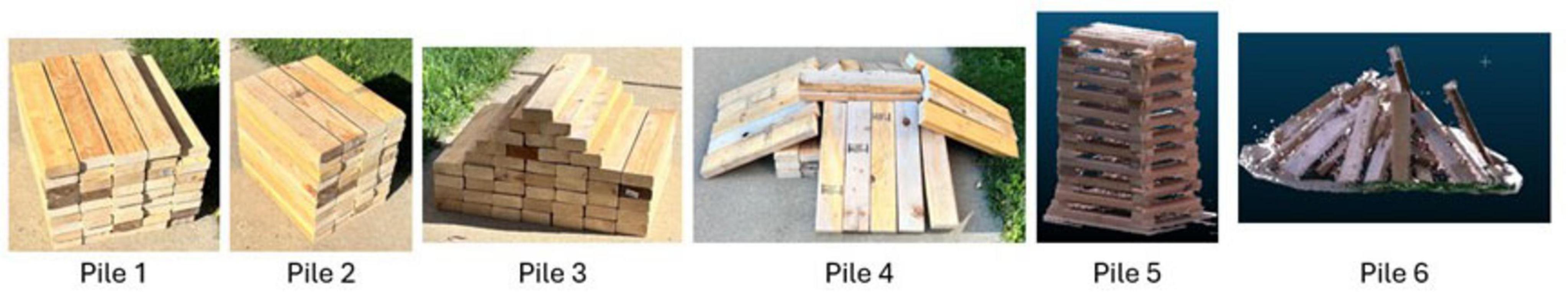
Figure 1. Synthetic piles.

2.2 Field piles

2.2.1 Site description

This study took place at HROS, which is maintained by the Boulder County Parks and Open Space, west of Lyons, Colorado and is part of the Colorado Front Range Wildfire Crisis Strategy landscape. The piles are located on 44.11 ha in a forested area that is dominated by ponderosa pine (Pinus ponderosa var. scopulorum). The piles were constructed in 2023, with no prior prescribed fire. Trees in this area were cut as part of a first entry for restoration prescription, with no material removed from the area, only formed into piles to burn. The last reported wildfire in this location was in 1867. Soil in this area is predominantly gravelly sandy loam about 0.5 m in depth (N. Stremel, personal communication, 29 Jan. 2025).

2.2.2 Field Pile data collection

In total, 15 piles were selected at HROS. Each pile was weighed and scanned using TLS; see Figure 2 for locations. HROS has 1881 piles that are planned to be burned in the winters of 2024–2026. Piles selected to be scanned and weighed were chosen with different shapes and sizes, in order to ensure variety in the sample. However, machine piles (greater than 178 cm × 381 cm) were excluded from sampling to make sure there was enough time to scan and weigh multiple piles as scanning and weighing large piles can take many hours. Each pile was scanned four times, once from each side. Our sampling protocol was chosen to allow flexibility in determining scan locations to minimize occlusion from vegetation. The scans were completed using a Leica BLK360 (Leica Geosystems, Heerbrugg, Switzerland), as described by Pokswinski et al. (2021). The scanner has an 830 nm laser wavelength, a maximum range of 60 m, covers 360° horizontally and 300° vertically, and weighs 1 kg. I used the standard sampling density with non-HDR imaging, which has a resolution of 10 mm at 10 m and a scan time of less than 4 min (Loudermilk et al., 2023; Leica Geosystems, BLK360 Spec Sheet, 2019/2022). For each pile, four spikes with pink flagging were placed around the perimeter of the pile forming a square (see Supplementary Figure 1) to make combining each pile scan easier. Each pile was then taken apart (Supplementary Figure 8) and weighed using a luggage scale (Travelon, Franklin Park, IL) and the geometric volume and mass of those piles were calculated using the methodology described in Wright et al. (2009). This methodology was developed by measuring the geometric and surface shape volume of 121 piles in the western US. The geometric volumes were calculated using equations adapted from Hardy (1996). Of note, this method typically underestimates the true pile volume for very small piles and overestimates the true volume for larger piles (Wright et al., 2009).

FIGURE 2

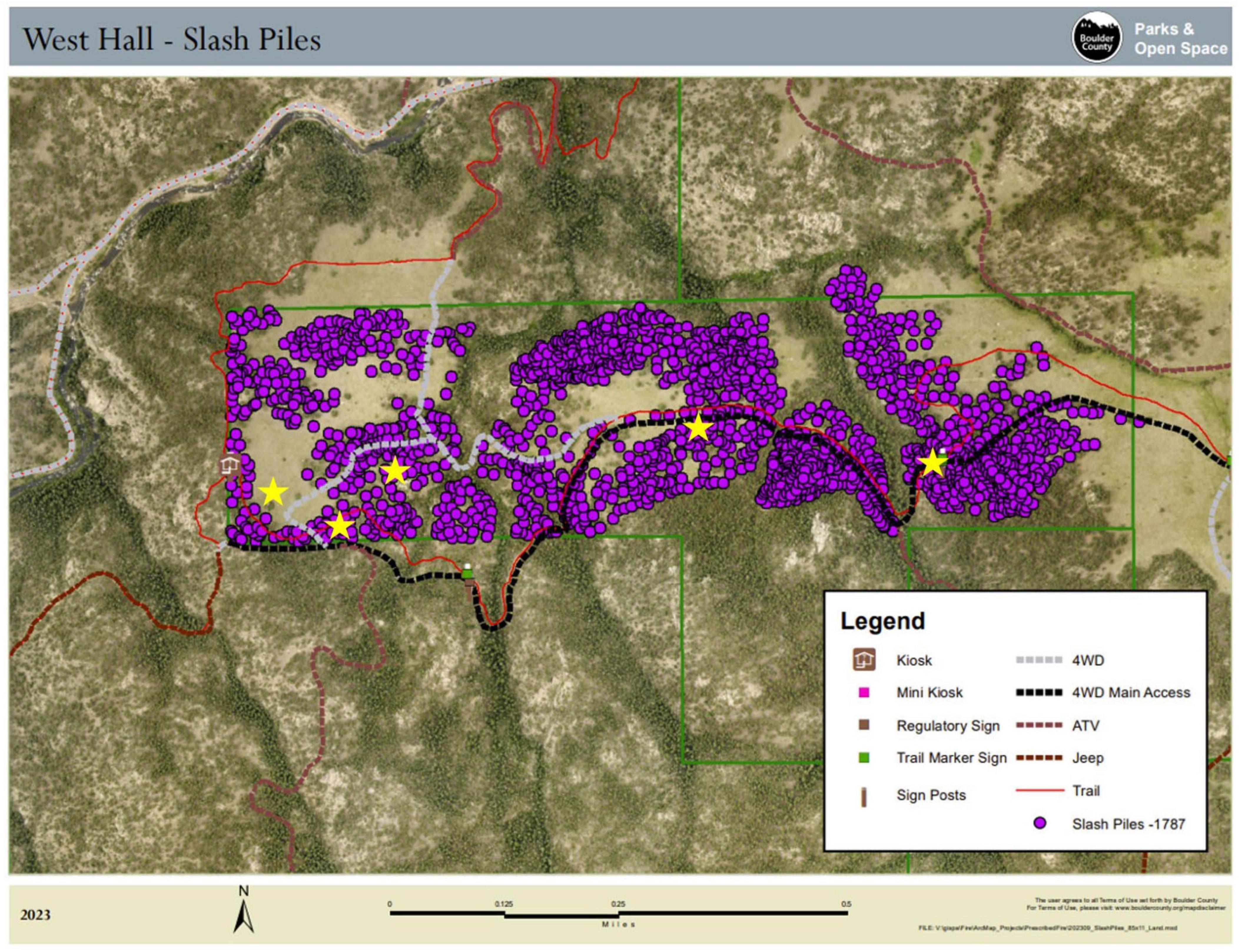
Figure 2. Pile Locations at Hall Ranch Open Space (HROS). Yellow stars are locations in which piles were measured.

2.3 TLS scan processing

Terrestrial laser scanning of the piles from both the field and the synthetic piles were uploaded using Cyclone REGISTER 360 Plus to convert the files on the BLK from. blk to .ptx files. The .ptx files are stitched together into a single point cloud and segmented to isolate only the pile using CloudCompare. The method used to stitch the scans for both handmade and field piles is described in detail in Table 1.

TABLE 1

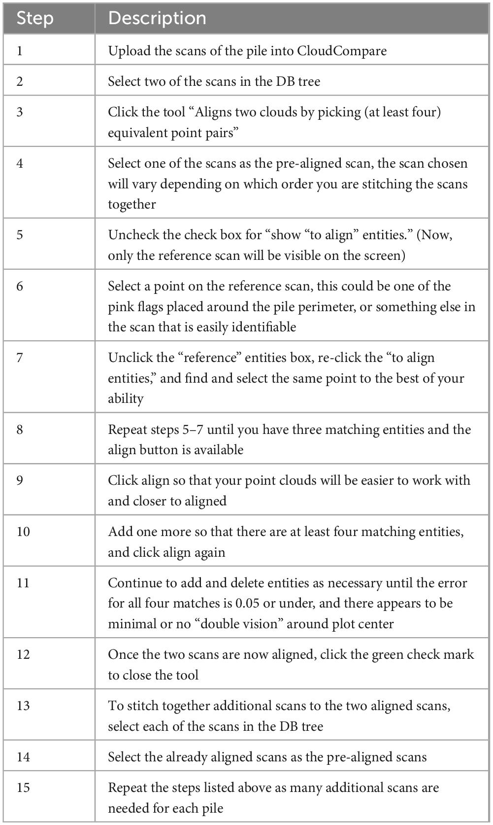
Table 1. Stitching description.

Once the scans have been stitched, the pile needed segmented, from the larger point cloud. The segmenting process is outlined in Supplementary Figure 2 and he often takes more than two iterations.

Following the segmentation of the pile from the larger point cloud, the volume for each pile point cloud was estimated using Poisson Recon Plugin in CloudCompare. To use the Plugin, normal must be computed for the point cloud, this accessed via “Edit> Normals> Compute.” This plug-in then creates a solid surface over the point cloud and allows you to turn it into a solid mesh. The solid mesh produces a scalar field where the color indicates the number of points in the point cloud (red representing the highest point density and blue representing the lowest point density) and allows the user to get rid of spaces on the solid mesh where there are not as many points registered by the TLS. This step ensures that the user is only calculating the volume of the actual pile. For each field pile, space colored in blue or green (green has the next fewest point density following blue) were removed from the pile. To remove the space colored in blue and green, when using the Plugin, ensure that “output density as SF” is selected. Then the user can remove the blue and green colored spaces under “Properties > SF display params.” CloudCompare has a function that will then estimate the volume of the solid mesh. This function is accessed via “Edit > Mesh > Measure volume.” There is no further point cloud reconstruction required.

2.3.1 Synthetic piles TLS scan processing

Each of the synthetic piles were scanned four times, once on each side, and this process was repeated twice. TLS scans for each pile were positioned approximately 2–3 m away from the pile. Scanning each synthetic pile twice in total allowed us to estimate any error associated with the TLS scans on the same shapes of the synthetic piles.

To explore the impact of stitching order on volume estimation, we explored all possible orders given the four scanned sides. Table 2 summarizes those stitching orders. The dash indicates the scans being stitched. So, 1-2 means that scans 1 and 2 are stitched together first, and 12-3 means that scans 1 and 2 which are already aligned, are stitched to scan 3.

TABLE 2

Table 2. Stitching combinations used on each of the synthetic piles.

2.3.2 Field piles TLS scan processing

Each field pile was also scanned four times, once on each side. TLS scans for each pile were positioned approximately 2–3 m away from the pile. Each field pile was stitched together 15 times. The different stitching orders are shown below in Table 3, the stitching combinations represent the scans that were stitched together to estimate the pile mass. Scan 1 represents the 1^st scan done of the pile, while the 4^th scan is the last scan done of the pile. The scans are completed sequentially in a circle around the perimeter of the pile. The location of the first scan was chosen at random, and the second scan was done adjacent to the location of the first scan.

TABLE 3

Table 3. Stitching combinations used on each of the field piles.

For each of the piles, the mass was estimated using a varying number of sides; 1, 2, 3, and all 4 sides of each pile. To estimate the mass of a pile using only one scan, there are four different mass estimates, using each side of the pile scans. To estimate the mass of a pile using two scans, there are six different stitching combinations that can be used. To estimate the mass of a pile using three scans, there are four different stitching combinations that can be used. Finally, to estimate the mass of a pile using all four scans, there is only one stitching combination. Each of the combinations was completed for each pile in order to see how the selection of different numbers and orientations of scans would influence the mass estimate of the pile.

The resulting volume estimation for each field pile was multiplied by a bulk density value of 76.79 kg/m³ (Wright et al., 2009), for hand piles in coniferous forests of Washington and Oregon. Due to the similarity of the species composition and the construction of the piles we have in Colorado and the lack of geographically explicit bulk density estimates, we chose to use the bulk density calculated by Wright et al. (2009) in our analysis. Bulk density is the mass of the material in the pile divided by the total space that the pile occupies, which includes empty space between the fuel in the pile.

The bulk density of the synthetic piles without any empty space is 415 and 116 kg/m³ for Pile 6 which was our attempt to mimic real-life conditions. Our bulk density values are much larger compared to the bulk density of conifer piles, indicating that there is much more empty space in the field piles. This mass estimation process was repeated for each of the 15 stitching orders across 16 field piles.

2.4 Statistical analyses

For the analysis of both the synthetic and field piles, we use the following metrics to compare the accuracy of TLS in predicting pile volume and mass to the actual known volume and mass. Additionally, these metrics are used to understand the impact of the user, stitching order, and scanning trial on the predicted volume of the synthetic piles.

The root mean squared error (RMSE) (Equation 1), mean bias error (MBE) (Equation 2), correlation coefficients (calculated in MATLAB using a built in function), mean absolute percent error (MAPE) (Equation 3), percent errors (Equation 4), relative errors (Equation 5), and relative differences (Equation 6) were calculated for each group of pile mass estimates. All analyses were completed in MATLAB. N is the number of samples in the sample size, x_i is the actual measurement and ${\widehat{x}}_i$ is the predicted measurement.

$RMSE=\sqrt{{\sum }_{i=1}^N{(x_i-\widehat{x_i})}^2/N}(1)$

$MBE=\frac{1}{N}{\sum }_{i=1}^N({\widehat{x}}_i-x_i)(2)$

$MAPE=100*\frac{1}{N}*{\sum }_{i=1}^N(x_i-\widehat{x_i})/\widehat{x_i}(3)$

$\%Error=(x_i-\widehat{x_i})/\widehat{x_i}*100(4)$

$RelativeError=(x_i-\widehat{x_i})/\widehat{x_i}(5)$

$RelativeDifference=(x_1-x_2)/((x_1-x_2)/2)(6)$

3 Results

The following section includes comparisons between the estimated mass values for the field piles and estimated volumes for the synthetic piles. Additionally, the field pile mass estimates were compared to both the mass estimates using the methodology developed by Wright et al. (2009) and the actual pile masses.

3.1 Synthetic piles

3.1.1 Synthetic pile measurements

Figure 3 shows the actual and estimated volumes for each of the synthetic piles as well as the volume of empty space in each pile. Table 4 summarizes the comparison between actual and estimated volume for each pile. The green circle is the actual measured volume of the pile, whereas the red points are volume estimates from the TLS scans. The different shapes of the red points indicate the trial and stitching order. So, Volume_T1_O1 is the volume estimated from trial 1 of the pile scans, and the 1^st stitching order. Whereas Volume _T2_O4 is the volume estimated from trial 2 of scans, and the 4^th stitching order. Each stitching order is described in Table 1. The different shades of red represent the same stitching order and trial done by an additional person. For all synthetic piles except synthetic pile 5, the volume estimates were consistent for both people. However, for Pile 5, one person was able to more accurately estimate the pile volumes while the other was not.

FIGURE 3

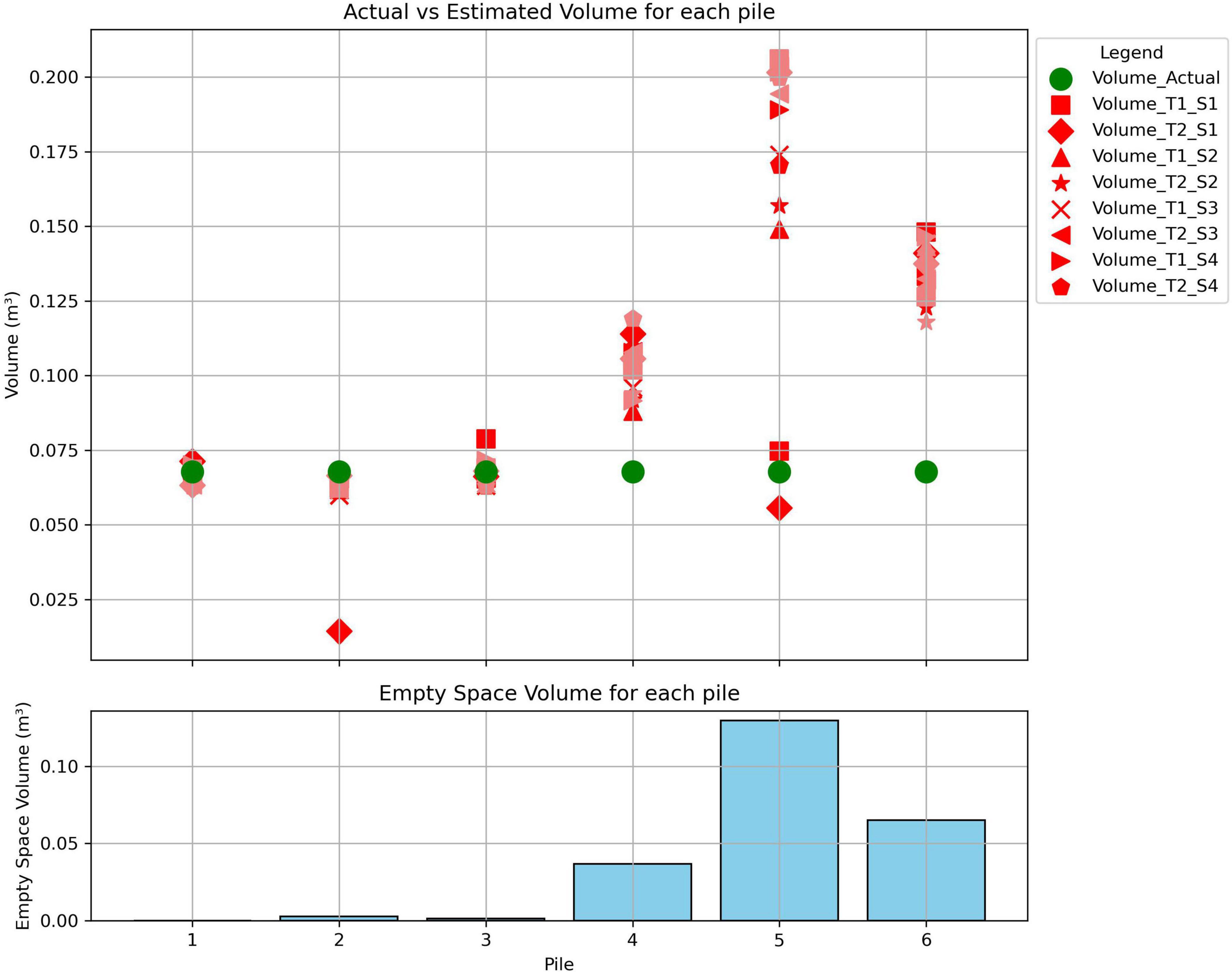
Figure 3. Actual vs. estimated volume for each synthetic pile and empty space volume.

TABLE 4

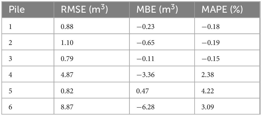
Table 4. Root mean squared error (RMSE), mean bias error (MBE), and mean absolute percent error (MAPE) of estimated mass values for synthetic piles.

Piles 1–3 had the most accurate volume predictions; they had the lowest RMSEs, MBEs, and MAPES compared to piles 4–6. However, the RMSE and MBE for pile 2 were higher than expected since for trial 2 and 2^nd stitching order, the volume estimate was much lower than the actual volume. The reason behind this error is unknown, and that stitching order was repeated several more times for that pile and still had the same results. Volume estimates for piles consistently overestimated the actual volumes of the piles. The inconsistent estimates for the masses for each pile based on both the stitching order as well as the trial does indicate that there is some error associated both with the stitching process as well as in the TLS scans. However, since the differences in the estimates are not consistent in either under or overestimating the synthetic pile mass, this means that there is no bias associated with the stitching process. Based on the results above, when there is any empty space in the synthetic pile, the TLS underestimated the volume of fuel compared to synthetic piles with minimal empty space, and the pile with the largest volume of empty space, had the largest errors. Additionally, synthetic piles with empty space had higher associated RMSEs and MAPEs.

3.1.2 Synthetic pile error

For the synthetic piles, we calculated the relative error when comparing each of the stitching orders to the actual pile volume, the relative difference between users for the volume estimates, as well as the relative error between trials across both users. These results are shown in Supplementary Figures 3–5, respectively.

For the stitching orders with adjacent stitching being done first, orders 1 and 2, the median relative errors when comparing each of the stitching orders to the actual pile volume, were 0.08 and 0.14, respectively (Supplementary Figure 3). For the stitching orders with opposite sides being stitched first, orders 3 and 4, the median relative errors were 0.17 and 0.24, respectively. Stitching orders with opposite sides stitched together first had higher median relative errors.

For all piles, except pile 5, the median relative error between users was less than 0.01 (Supplementary Figure 4). This result means that there was not a bias associated with one user versus another (except for Pile 5). Additionally, when looking at the spread of relative errors between users for each pile there was less user difference for the solid piles (Piles 1–3) than the piles with significant empty space. Using Piles 4 and 6 as reasonable real-world mimics, we can assess the random relative error, or uncertainty, associated with employing different users to determine pile volumes to be the standard deviation of the relative error. For our case study, that random relative error for each pile is as follows, 0.05, 0.46, 0.06, 0.11, 0.43, 0.09; therefore, the random relative error associated with using different users to stitch scan is ∼0.10 or 10%.

Each of the median relative errors between trials (Supplementary Figure 5) were all less than 0.07, the standard deviation of these relative errors can be considered the uncertainty associated with a measurement repeat (but the process and user stay the same); that uncertainty for each pile is as follows, 0.05, 0.47, 0.08, 0.11, 0.13, 0.09. The one anomaly for Pile 2 is increasing the random relative error estimate for that pile; however, there appears to be no difference between solid piles (Piles 1–3) and piles with empty space (Piles 4–6). In general, the random relative error associated with repeat trials is ∼0.10 or 10%, similar to the uncertainty associated with having different users stitch piles.

3.2 Field piles

Figure 4 shows the mass estimates for each pile using TLS as well as the method developed by Wright et al. (2009) compared to the actual mass of the pile weighed by hand. As mentioned in the methods section, each of the piles had 15 different mass estimates based on the varying stitching order. However, Figure 4 only shows the mass estimates of one stitching order for each number of scans. In other words, only one stitching order is being shown here for the mass estimated using three scans. Supplementary Figure 6 in the supplemental shows the 15 different mass estimates for only Field Pile 1, to show the variability between the different TLS mass estimations. There is variability associated with the chosen stitching order and the number of sides selected to estimate the pile mass. This same analysis was done with each of the different stitching orders and similar results were obtained for each. Looking at all piles, for estimating the mass using three scans, when the first stitching done is opposite, the mass estimate was less accurate compared to the mass estimate where the first stitching done is adjacent to one another. For estimating the mass using two scans, when the first stitching done is opposite, the mass estimate was more accurate compared to the mass estimate where the first stitching done is adjacent to one another. For example, the percent errors when stitching together opposite sides first using three sides, the median percent error was 44% compared to a percent error of 15% when stitching together adjacent sides first. When using two sides, the percent error when stitching opposite sides first was 9% while stitching adjacent sides first had a percent error of 25%.

FIGURE 4

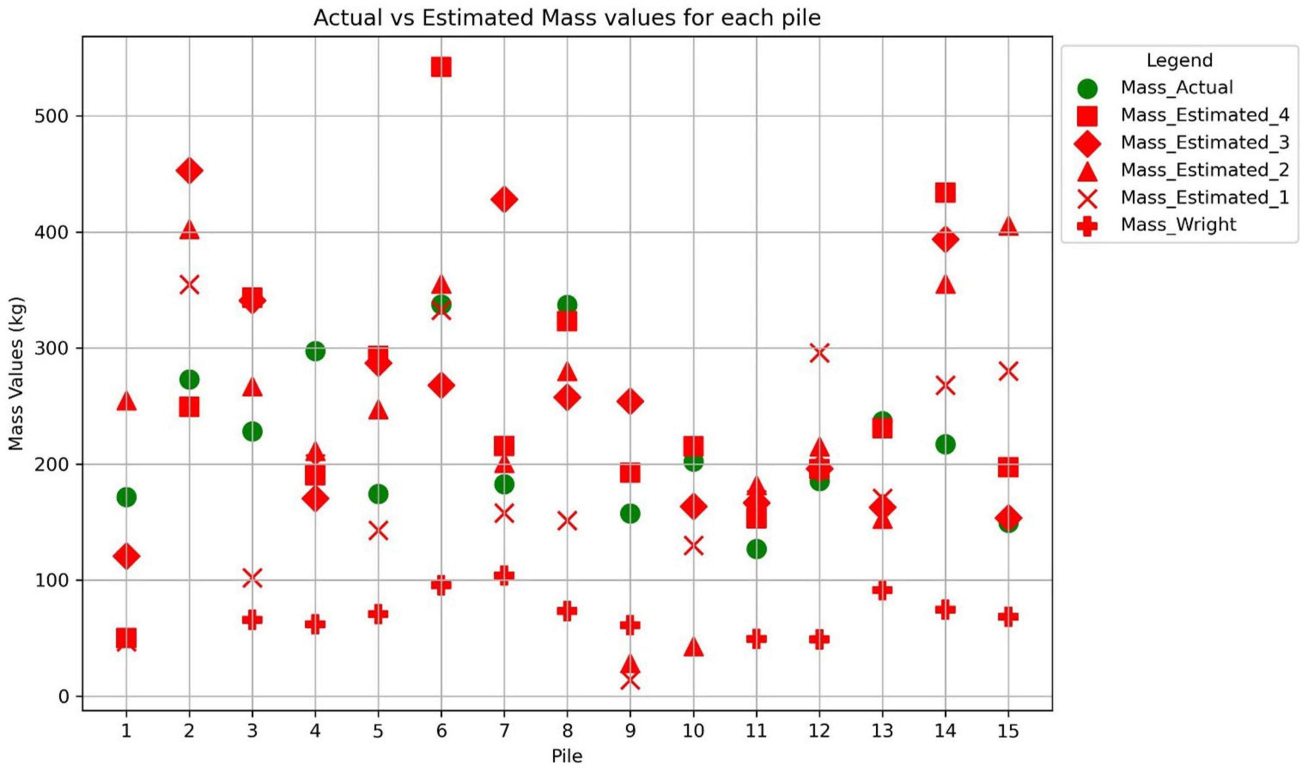
Figure 4. Actual vs. estimated mass values for each pile. Actual pile masses compared to estimated pile masses using methods developed by Wright et al. (2009) and the terrestrial laser scanning (TLS). For three sides the stitching order is 123 and for two sides the stitching orders, refer to Supplementary Figures 6, 7.

In Figure 4, the actual weighed mass is represented with a green circle, whereas the estimated mass values are all shown in red. For Mass_Estimated_X, the number represents the amount of sides that were stitched. Mass_Estimated_4 means that all four sides of the pile were stitched and used to estimate the pile mass, whereas Mass_Estimated_1 means only one side of the pile was used to estimate the pile mass. Note that the measurements needed to be collected in order to estimate the mass using the methodology developed by Wright et al. (2009); however, for this study, for piles 1, 2, and 10, we did not follow that approach, so we do not include that estimate for those three piles. The Wright mass estimates consistently underestimated the actual masses of the piles, meaning this is a biased estimate. From this plot it is evident that neither the TLS or the previous methodology from Wright are consistently accurate in predicting the individual pile masses. There is no consistent pattern between the masses estimated using the TLS and the actual masses of the piles. Additionally, there is no consistent pattern associated with the number of sides scanned and stitched.

Figure 5 shows the estimated vs. actual pile masses when using the different number of sides to estimate the pile masses. Table 5 shows the ranges of RMSE, MBE, correlation coefficients, and MAPE for the in-field pile data shown in Figure 5. There is little correlation between the actual and estimated masses regardless of the number of sides stitched. Stitching all four sides was the most correlated with the individual pile masses, however, the R² value is still low. The RMSEs and MBEs were all fairly high regardless of the number of sides stitched, ranging from 51 to 159 kg, which in some cases was more than half of the weight of the actual pile mass. Figure 5 and Table 5 highlight the inability of TLS to accurately predict a single pile mass.

FIGURE 5

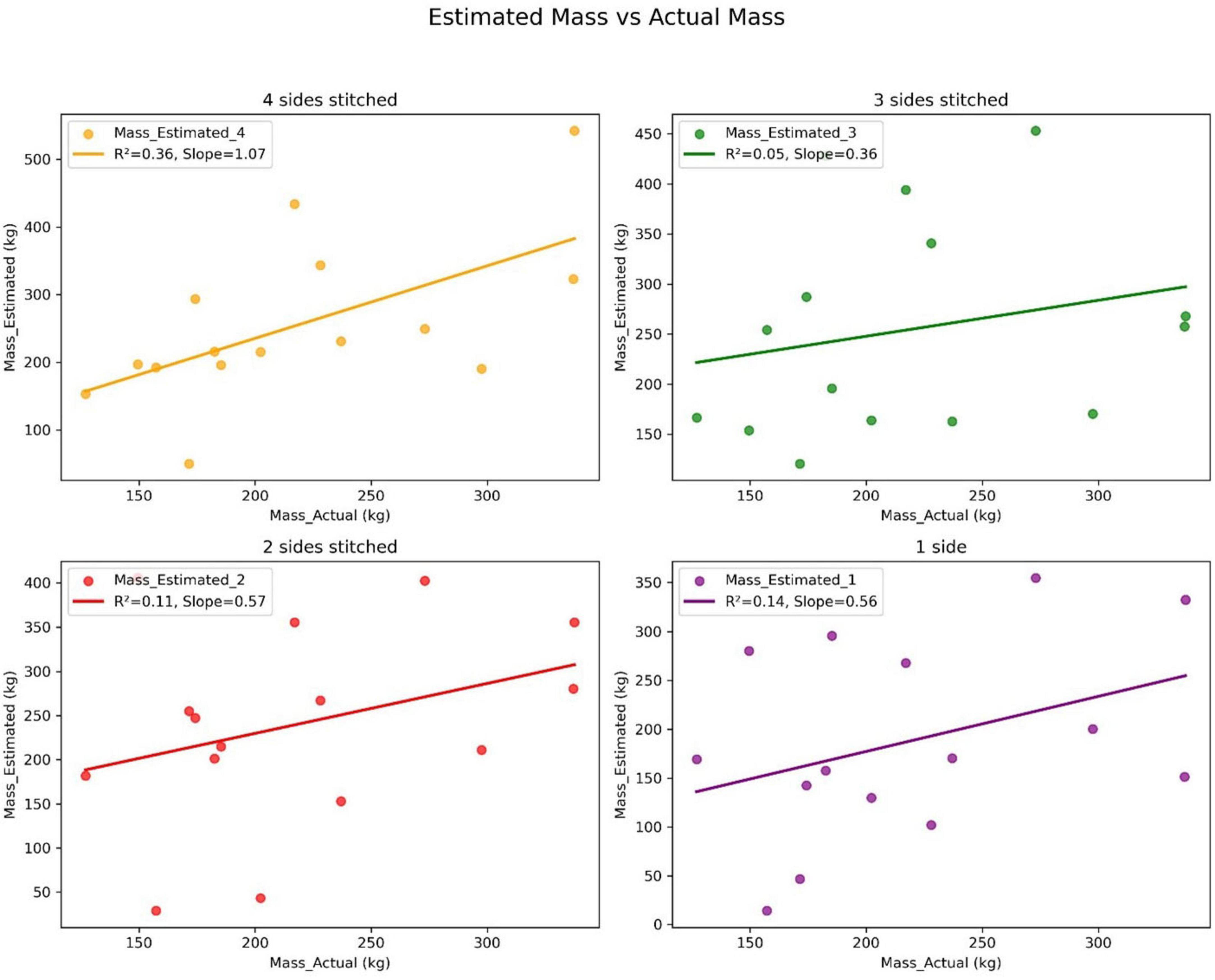
Figure 5. Estimated pile mass vs. actual pile mass. The stitching order is as follows, estimating the mass using three sides, 123, estimating the mass using two sides, 13, estimating the mass using one side, scan one was used.

TABLE 5

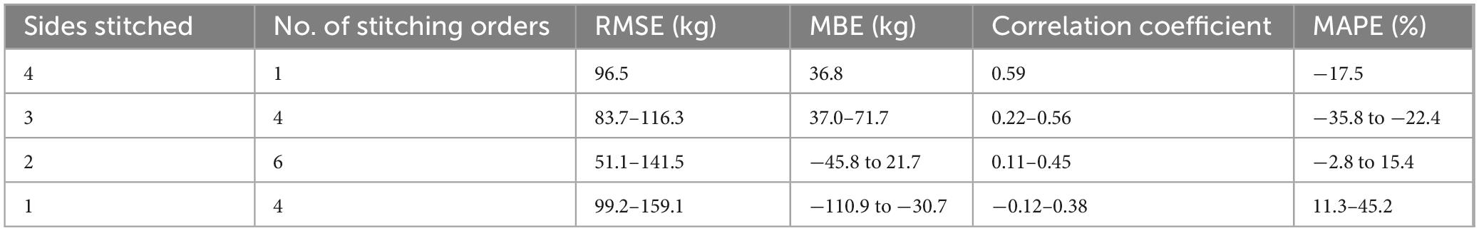
Table 5. Root mean squared error (RMSE), mean bias error (MBE), and correlation coefficients of estimated mass values for in-field piles.

Figure 6 shows the percent error between the actual and estimated masses for the field piles as well as the estimated masses using the methodology developed by Wright et al. (2009). For each mass prediction method, only one stitching combination is being used in this analysis, however, this analysis was completed for each of the additional stitching combinations. When using three sides of the pile to predict pile mass, the percent error was the lowest across all piles when the scans were in sequential order, for example, scans 123 and scans 234. When using two sides of the pile to estimate the mass, the percent difference was the lowest for stitching combinations that were opposite of each other, for example, 13 and 24. In each case, regardless of the number of sides stitched to predict the pile mass, they were not consistent in either over or underestimating the pile masses, meaning that this measurement is not biased. As shown in Figure 5, the TLS is not accurate in estimating the mass of a single pile, but over the entire sample size (Figure 6), the median percent error across all piles is near 0.

FIGURE 6

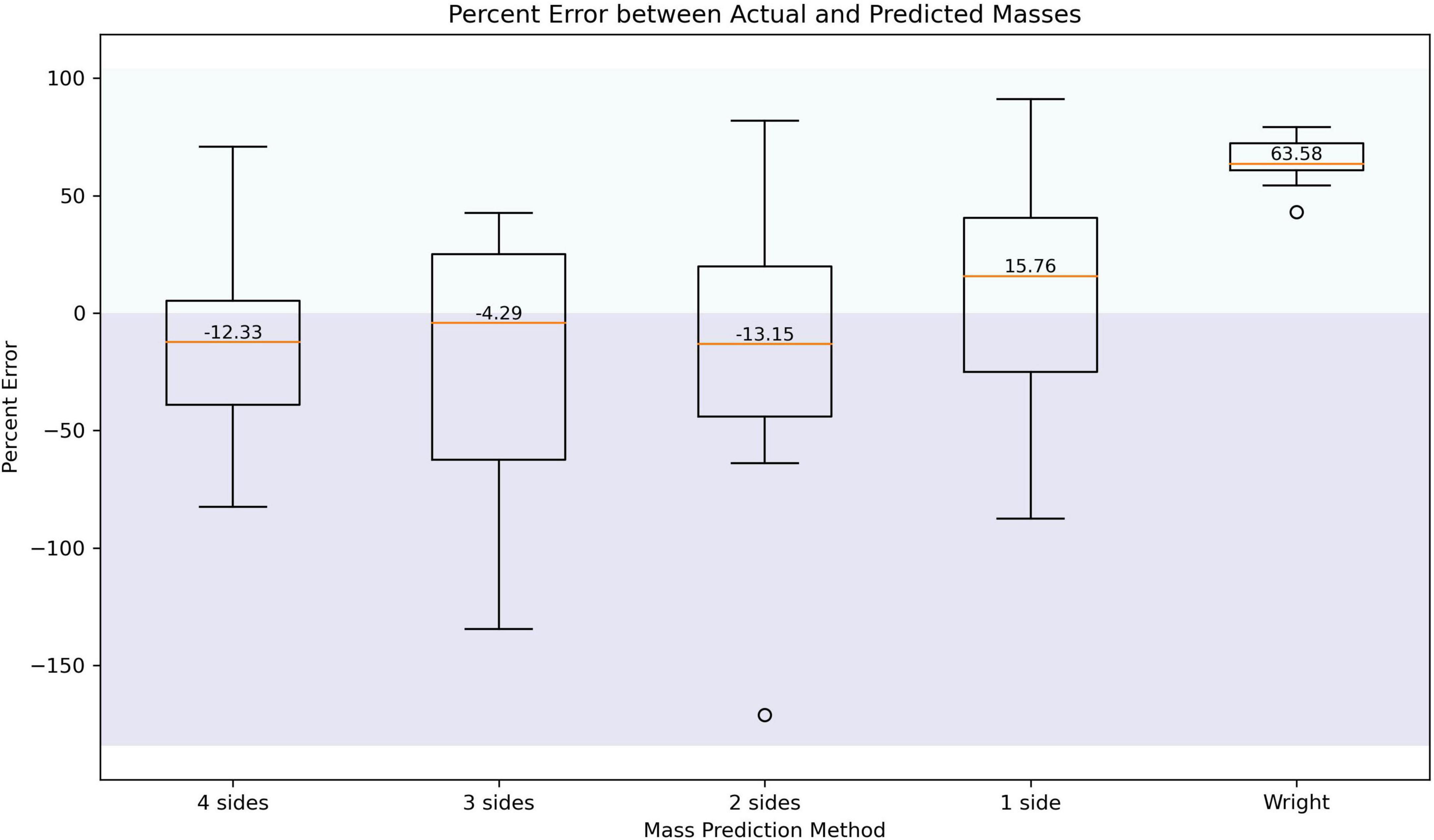
Figure 6. Percent error between actual and estimated pile masses. The stitching order is the same as in Figure 4.

4 Discussion

Using TLS to estimate pile mass reduces the bias in the estimated mass compared to previous pile estimation techniques used by Wright et al. (2009). Using each of the different stitching methods from the TLS scans is not accurate for predicting a single pile mass, but for the entire sample size, the median percent error was lower compared to previous pile mass estimation techniques. Across multiple piles, TLS performed well in estimating pile masses. Similar to the results of both Long and Boston (2014); Casey et al. (2015), the TLS did a better job at estimating the volumes of piles compared to traditional volume estimation methods for “smaller” piles.

For synthetic piles, the difference between the users completing stitching did not influence the results much, ∼10% for piles that mimic real world. There was also not a big difference for repeats of the TLS scans, ∼10%. However, the stitching order did make a difference. Based on the comparison between stitching orders, orders that included stitching adjacent scans first (orders three and four) had higher relative errors. This is inconsistent with what was found for the field piles, where the estimates of pile masses using both three and two sides had lower relative errors when the scans were adjacent. Based on the stitching order results, we do not have any recommendations of which stitching order to use while stitching pile scans.

Being able to estimate the masses of large quantities of piles is crucial for land managers in understanding the treatment effect of prescribed fire. Land managers prioritize being able to estimate large numbers of piles and will rarely need to estimate the mass of only a single pile. Stitching three sides of a pile was overall the most accurate method to estimating the mass of all of the piles in total. However, all of the other stitching methods had a median percent error of less than 20%. Therefore, if there is not enough time to do three scans per pile, scanning either one or two sides of the pile will not result in a significant increase in error. Although using three sides had the lowest error when looking at all of the piles, using four sides had the highest correlation when predicting individual mass.

Although TLS had an overall lower mean percent error relative to previous methods, there are still constraints associated with operationalizing TLS for pile estimation. There is a time cost associated with the processing of the TLS scans. Future work could involve looking into ways to make the process of processing these TLS scans more efficient. Scanning a large sample of piles all at once could reduce the scanning time and time spent processing the scans. Additionally, this study had a relatively small sample size, 15 piles, on only one ecosystem. Future work that measures more piles across several ecosystems would be helpful to assess if the results are the same across a larger sample size and different locations.

For future work, there is a need for methods to actually predict pile masses. In future studies, the development of a quick (< 5 min) in-field measurement that could be used in combination with the TLS scans to predict pile masses may prove to be useful to prescribed fire implementers. TLS scans take less time than traditional field measurements, so any additional non time intensive field metrics that could help predict total pile masses could be helpful. Additionally, methods to calculate bulk density of piles could eliminate the need for a two-step process in mass prediction, as shown in this analysis. There are metrics that can be derived from point clouds such as height distributions, crown volume, vertical density profiles, as well as point return counts that have been used in previous studies to predict fuel types and fuel loading (Gallagher et al., 2024; Loudermilk et al., 2023). It would be interesting to assess the ability of those variables to help further predict the total mass of the piles.

Data availability statement

The raw data supporting the conclusions of this article will be made available by the authors, without undue reservation.

Author contributions

AG: Conceptualization, Data curation, Formal analysis, Investigation, Methodology, Writing – original draft, Writing – review & editing. MD: Data curation, Formal analysis, Investigation, Writing – review & editing. AF: Data curation, Investigation, Writing – review & editing. SH: Data curation, Investigation, Writing – review & editing. PH: Funding acquisition, Investigation, Supervision, Writing – review & editing. CH: Conceptualization, Formal analysis, Investigation, Resources, Supervision, Writing – review & editing. MH: Conceptualization, Formal analysis, Funding acquisition, Resources, Supervision, Writing – review & editing.

Funding

The author(s) declare that financial support was received for the research and/or publication of this article. This work was funded by the Strategic Environmental Research Development Program (SERDP) through grant RC20-1382 as well as the National Science Foundation Graduate Research Fellowship Program.

Acknowledgments

We thank the Hannigan Air Quality Lab at the University of Colorado Boulder and Chad Hoffman’s Lab at Colorado State University.

Conflict of interest

The authors declare that the research was conducted in the absence of any commercial or financial relationships that could be construed as a potential conflict of interest.

Generative AI statement

The authors declare that no Generative AI was used in the creation of this manuscript.

Any alternative text (alt text) provided alongside figures in this article has been generated by Frontiers with the support of artificial intelligence and reasonable efforts have been made to ensure accuracy, including review by the authors wherever possible. If you identify any issues, please contact us.

Publisher’s note

All claims expressed in this article are solely those of the authors and do not necessarily represent those of their affiliated organizations, or those of the publisher, the editors and the reviewers. Any product that may be evaluated in this article, or claim that may be made by its manufacturer, is not guaranteed or endorsed by the publisher.

Supplementary material

The Supplementary Material for this article can be found online at: https://www.frontiersin.org/articles/10.3389/ffgc.2025.1663753/full#supplementary-material

References

Andreae, M. O., and Merlet, P. (2001). Emission of trace gases and aerosols from biomass burning. Glob. Biogeochem. Cycles 15, 955–966. doi: 10.1029/2000GB001382

Crossref Full Text | Google Scholar

Arapaho and Roosevelt National Forests and Pawnee National Grassland. (2024). Resource management. Available online at: https://www.fs.usda.gov/detail/arp/landmanagement/resourcemanagement/?cid=fsm91_058292 (accessed December 10, 2024)

Google Scholar

Casey, J. M., Brooks, R., Eitel, J., and Keefe, R. (2015). Using logging residues as biofuel feedstocks in the Pacific Northwest: Estimating slash pile volumes with low-cost, lightweight terrestrial LiDAR. Master’s thesis. Idaho: University of Idaho.

Google Scholar

Cranmer, N., Han, T., Chedzoy, B., Smallidge, P. J., Beier, C., Johnson, L., et al. (2024). Estimating merchantable and non-merchantable wood volume in slash walls using terrestrial and airborne LiDAR. Forest Ecol. Manag. 569:122211. doi: 10.1016/j.foreco.2024.122211

Crossref Full Text | Google Scholar

Cross, J. C., Turnblom, E. C., and Ettl, G. J. (2013). Biomass production on the olympic and kitsap peninsulas, Washington: Updated logging residue ratios, slash pile volume-to-weight ratios, and supply curves for selected locations (PNW-GTR-872). Washington, DC: U.S. Department of Agriculture.

Google Scholar

Gallagher, M. R., Skowronski, N. S., and Loudermilk, E. L. (2024). Monitoring fuel loads and prescribed fire effects with terrestrial laser scanning. Washington, DC: U.S. Forest Service.

Google Scholar

González-Cabán, A. (2008). Proceedings of the second international symposium on fire economics, planning, and policy: A global view (PSW-GTR-208). Vallejo, CA: U.S. Department of Agriculture, Forest Service, Pacific Southwest Research Station, doi: 10.2737/PSW-GTR-208

Crossref Full Text | Google Scholar

Hardy, C. C. (1996). Guidelines for estimating volume, biomass and smoke production for piled slash (PNW-GTR-364). Corvallis, OR: U.S. Department of Agriculture, Forest Service, Pacific Northwest Research Station, doi: 10.2737/PNW-GTR-364

Crossref Full Text | Google Scholar

Kolden, C. A. (2019). We’re not doing enough prescribed fire in the Western United States to mitigate wildfire risk. Fire 2:30. doi: 10.3390/fire2020030

Crossref Full Text | Google Scholar

Long, J. J., and Boston, K. (2014). An evaluation of alternative measurement techniques for estimating the volume of logging residues. Forest Sci. 60, 200–204. doi: 10.5849/forsci.13-501

Crossref Full Text | Google Scholar

Loudermilk, E. L., Pokswinski, S., Hawley, C. M., O’Brien, J. J., Hudak, A. T., Hiers, J. K., et al. (2023). Terrestrial laser scan metrics predict surface vegetation biomass and consumption in a frequently burned southeastern U.S. ecosystem. Fire 6:151. doi: 10.3390/fire6040151

Crossref Full Text | Google Scholar

Miller, S., Rhoades, C., Schnackenberg, L., Fornwalt, P., and Schroder, E. (2015). Slash from the past: Rehabilitating pile burn scars. Fort Collins, CO: U.S. Department of Agriculture, Forest Service, Rocky Mountain Research Station.

Google Scholar

Mott, C. M., Hofstetter, R. W., and Antoninka, A. J. (2021). Post-harvest slash burning in coniferous forests in North America: A review of ecological impacts. Forest Ecol. Manag. 493:119251. doi: 10.1016/j.foreco.2021.119251

Crossref Full Text | Google Scholar

National Academies of Sciences, Engineering, and Medicine. (2022). Wildland fires: Toward improved understanding and forecasting of air quality impacts: Proceedings of a workshop. Washington, DC: The National Academies Press, doi: 10.17226/26465

PubMed Abstract | Crossref Full Text | Google Scholar

Pierobon, F., Sifford, C., Velappan, H., and Ganguly, I. (2022). Air quality impact of slash pile burns: Simulated geo-spatial impact assessment for Washington State. Sci. Total Environ. 818:151699. doi: 10.1016/j.scitotenv.2021.151699

PubMed Abstract | Crossref Full Text | Google Scholar

Pokswinski, S., Gallagher, M. R., Skowronski, N. S., Loudermilk, E. L., Hawley, C., Wallace, D., et al. (2021). A simplified and affordable approach to forest monitoring using single terrestrial laser scans and transect sampling. MethodsX 8:101484. doi: 10.1016/j.mex.2021.101484

PubMed Abstract | Crossref Full Text | Google Scholar

Roos, C. I., Rittenour, T. M., Swetnam, T. W., Loehman, R. A., Hollenback, K. L., Liebmann, M. J., et al. (2020). Fire suppression impacts on fuels and fire intensity in the western U.S.: Insights from archaeological luminescence dating in northern New Mexico. Fire 3:32. doi: 10.3390/fire3030032

Crossref Full Text | Google Scholar

Rosenberg, A., Hoshiko, S., Buckman, J. R., Yeomans, K. R., Hayashi, T., Kramer, S. J., et al. (2024). Health impacts of future prescribed fire smoke: Considerations from an exposure scenario in California. Earth’s Future 12:e2023EF003778. doi: 10.1029/2023EF003778

PubMed Abstract | Crossref Full Text | Google Scholar

Tenny, J. T., Sankey, T. T., Munson, S. M., Sánchez Meador, A. J., and Goetz, S. J. (2025). Canopy and surface fuels measurement using terrestrial lidar single-scan approach in the Mogollon Highlands of Arizona. Int. J. Wildland Fire 34:WF24221. doi: 10.1071/WF24221

Crossref Full Text | Google Scholar

Trofymow, J. A., Coops, N. C., and Hayhurst, D. (2014). Comparison of remote sensing and ground-based methods for determining residue burn pile wood volumes and biomass. Can. J. For. Res. 44, 182–194. doi: 10.1139/cjfr-2013-0281

Crossref Full Text | Google Scholar

U.S. Department of Agriculture, Forest Service. (2022). Confronting the wildfire crisis: A strategy for protecting communities and improving resilience in America’s forests. Washington, DC: U.S. Department of Agriculture, Forest Service.

Google Scholar

Wibbenmeyer, M., and Tastet, A. M. (2021). Wildfires in the United States 101: Context and consequences. Washington, DC: Resources for the Future.

Google Scholar

Woolsey, G. A., Tinkham, W. T., Battaglia, M. A., and Hoffman, C. M. (2024). Constraints on mechanical fuel reduction treatments in United States Forest Service wildfire crisis strategy priority landscapes. J. For. 122, 335–351. doi: 10.1093/jofore/fvae012

Crossref Full Text | Google Scholar

Wright, C. S., Balog, C. S., and Kelly, J. W. (2009). Estimating volume, biomass, and potential emissions of hand-piled fuels (PNW-GTR-805). Corvallis, OR: U.S. Department of Agriculture, Forest Service, Pacific Northwest Research Station, doi: 10.2737/PNW-GTR-805

Crossref Full Text | Google Scholar