Modeling the COVID-19 Epidemic With Multi-Population and Control Strategies in the United States

As of January 19, 2021, the cumulative number of people infected with coronavirus disease-2019 (COVID-19) in the United States has reached 24,433,486, and the number is still rising. The outbreak of the COVID-19 epidemic has not only affected the development of the global economy but also seriously threatened the lives and health of human beings around the world. According to the transmission characteristics of COVID-19 in the population, this study established a theoretical differential equation mathematical model, estimated model parameters through epidemiological data, obtained accurate mathematical models, and adopted global sensitivity analysis methods to screen sensitive parameters that significantly affect the development of the epidemic. Based on the established precise mathematical model, we calculate the basic reproductive number of the epidemic, evaluate the transmission capacity of the COVID-19 epidemic, and predict the development trend of the epidemic. By analyzing the sensitivity of parameters and finding sensitive parameters, we can provide effective control strategies for epidemic prevention and control. After appropriate modifications, the model can also be used for mathematical modeling of epidemics in other countries or other infectious diseases.

Introduction

Coronavirus disease-2019 (COVID-19) is a contagious disease caused by severe acute respiratory syndrome coronavirus 2 (SARS-CoV-2). Anyone can have mild to severe symptoms. Older adults and people who have severe underlying medical conditions like heart or lung disease or diabetes seem to be at higher risk of developing more serious complications from COVID-19 illness. People with COVID-19 have had a wide range of symptoms reported ranging from mild symptoms to severe illness. Symptoms may appear 2–14 days after exposure to the virus. People with these symptoms may have COVID-19: fever or chills, cough, shortness of breath or difficulty breathing, and so on (1).

The first case was identified in Wuhan, China, in December 2019. It has since spread worldwide, leading to an ongoing pandemic. As of January 19, 2021, the total number of confirmed cases worldwide has reached 96,158,807, and the death toll has reached 20,570,050. Among them, the cumulative number of people infected with COVID-19 in the United States is as high as 24,433,486, and the number is still rising. In addition, with the emergence of mutant virus strains in the United Kingdom that spreads more easily and quickly than the other variants (2), it may make the epidemic prevention situation more severe. Mathematical modeling is one of the most effective methods for forecasting of infectious disease outbreaks and, thus, yielding valuable insights to suggest how future efforts may be improved. An important method for epidemiological studies of such acute infectious diseases is mathematical modeling (3–6). Therefore, it is necessary to establish a mathematical model to accurately predict the evolution trend of COVID-19 in the United States, and find key factors that can significantly affect the evolution of COVID-19 to provide effective control strategies.

At first, many scholars established mathematical modeling research on COVID-19 in China (7–12). For example, Wu et al. (8) proposed a four-dimensional ordinary differential equations to research on the epidemic in Wuhan at the beginning, and the estimated basic reproductive number was 2.68. Besides, they also estimated the number of imported infections from Wuhan to some major cities in China. In the following, Kucharski et al. (7) fitted a stochastic transmission dynamic model with data which includes the cases in Wuhan and internationally exported cases from Wuhan, and estimated that the basic reproductive number declined from 2.35 to 1.05

With the spread of COVID-19 around the world, many scholars were also mathematically modeling the evolution trend of the epidemic in the United States, Britain, Italy, and other countries (13–23). For instance, Reiner et al. (13) used a deterministic susceptible-exposed-infectious-recovered (SEIR) compartmental framework to model the COVID-19 infections in the United States at the state level and assessed scenarios of social distancing mandates and levels of mask use. Giordano et al. (16) established a relatively comprehensive model with eight variables, which included susceptible (S), infected (I), diagnosed (D), ailing (A), recognized (R), threatened (T), healed (H), and extinct (E). The infected individuals were distinguished based on the severity of their symptoms and if they were diagnosed or not.

Unfortunately, the aforementioned models failed to consider individuals who are asymptomatic and undiagnosed in modeling the COVID-19 epidemic in the United States, and no theoretical support was provided for the sensitivity analysis of parameters. This may limit the accuracy of forecasting and the reliability of results.

To resolve this problem, this study presents a novel epidemic model, which divided the population into the Susceptible (S), Asymptomatic and undetected (A), Asymptomatic and detected (A_D), Symptomatic and infected (I), recovered (R) and death (D) groups. Besides, we also use a global sensitivity analysis method to compute the sensitivity indexes of all parameters in order to provide theoretical support for parameter sensitivity and verify it by numerical simulations.

Methods

Mathematical Model

Here is an overview of the transmission mechanism of COVID-19 in the population (Figure 1):

FIGURE 1

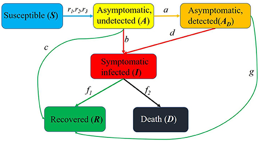
Figure 1. Schematic diagram of the spread of the epidemic in United States. S(t) is the susceptible, A(t) is the asymptomatic and undetected, A_D(t) is the asymptomatic and detected, I(t) is the symptomatic and infected, R(t) is the recovered and D(t) is the death.

It should be noted that the birth rate of newborns and the natural mortality rate of the population were ignored in this study.

The first subject is the susceptible population S(t). Because the birth rate of newborns was ignored, there is no source of the susceptible population, and the output includes contacts of susceptible people and asymptomatic undiagnosed people, asymptomatic diagnosed people, and symptomatic infected people. The infection rates are r₁, r₂, r₃, respectively.

Followed by the asymptomatic untested population A(t), whose sources are contacts among susceptible people and asymptomatic undiagnosed people, asymptomatic diagnosed people, and symptomatic infected people. Then, the input includes r₁S(t)A(t), r₂S(t)A_D(t), r₃S(t)I(t), and the outputs are the asymptomatic undiagnosed people will be diagnosed as asymptomatic people with probability a, be diagnosed as a symptomatically infected population b, and with probability c to develop into a cured population.

The source of the asymptomatic diagnosed population A_D(t) is the asymptomatic undiagnosed population that will be diagnosed as asymptomatic diagnosed population with probability a. The output includes the development of symptomatic infection population with probability d and the cure with probability g.

The sources of symptomatic infected population I(t) include the asymptomatic undiagnosed people with probability b to develop into symptomatic infected population and asymptomatic diagnosed people with probability d to develop into symptomatic infected population. The output includes part of the symptomatically infected people are cured with probability f₁, and part of them died with probability f₂.

The source of the recovered population R(t) includes three parts: first, the asymptomatic undiagnosed population is cured with probability c, the second is the asymptomatic diagnosed population is cured with probability g, and the third is the symptomatic infected population is cured with probability f₁.

Without considering the natural death of the population, the source of the death population D(t) is the development of the symptomatic infection population with probability f₂.

Therefore, this study proposed a mathematical model with Susceptible (S), Asymptomatic and undiagnosed (A), Asymptomatic and diagnosed (A_D), Symptomatic and infected (I), recovered (R) and death (D) groups.

$\begin{array}{l}\frac{dS(t)}{dt}=-r_{1}S(t)A(t)-r_{2}S(t)A_D(t)-r_{3}S(t)I(t),\\ \frac{dA(t)}{dt}=r_{1}S(t)A(t)+r_{2}S(t)A_D(t)+r_{3}S(t)I(t)\\ -aA\mathrm{(t)}-bA\mathrm{(t)}-cA\mathrm{(t)}\text{, }\\ \frac{d{A}_D(t)}{dt}=aA(t)-d{A}_D(t)-g{A}_D(t),\\ \frac{dI(t)}{dt}=bA(t)\text{+}d{A}_D(t)-(f_1+f_2)I(t),\\ \frac{dR(t)}{dt}=cA(t)+g{A}_D(t)+f_{1}I(t),\\ \frac{dD(t)}{dt}=f_{2}I(t).& (1)\end{array}$

In the above equation (1), S(t), A(t), A_D(t), I(t), R(t), D(t) represent the susceptible population, asymptomatic undiagnosed population, asymptomatic diagnosed population, symptomatic infected population, recovered population, and death population in the United States at time t, respectively.

Model Parameter Estimation

We infer the model parameters based on the baidu data in United States from February 22, 2020 (day 1) to January 10, 2021 (day 324). The data from February 22, 2020 to December 1, 2020, which were used for the training set, are provided in Table 1 and were turned into fractions over the whole United States population (~3 ×10⁸) for simulations.

TABLE 1

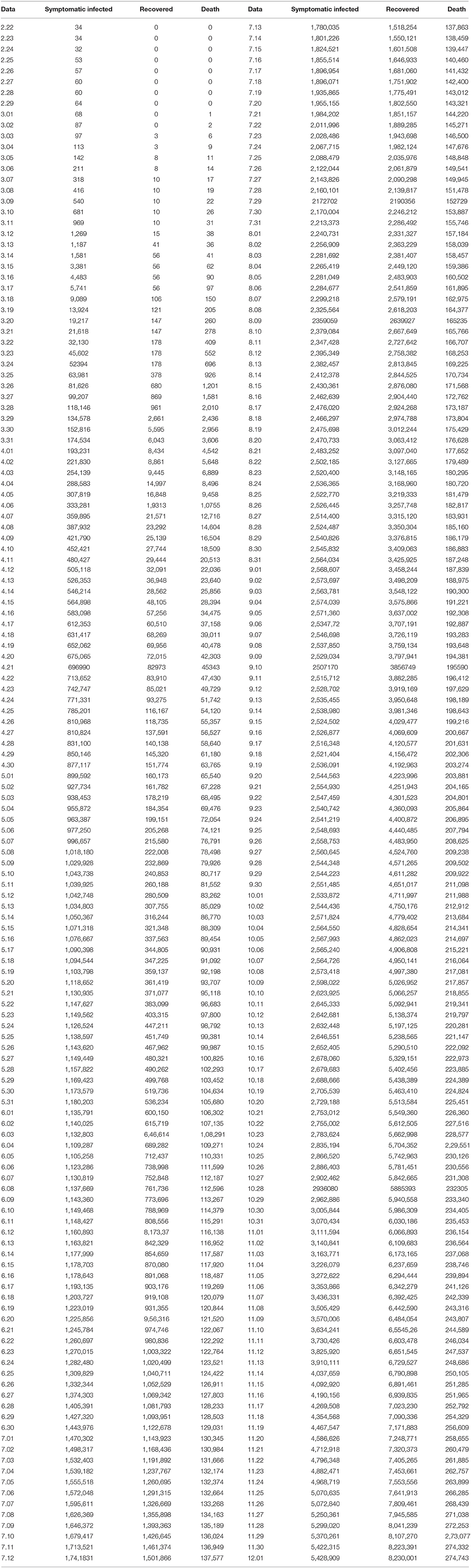
Table 1. The training set for model parameter estimation.

The estimated parameter values are based on the gathered data which are the number of currently infected individuals I(t), the number of diagnosed individuals who recovered R(t) and the number of death D(t) because of SARS-CoV-2 virus.

The nonlinear least square (NLS) method is regarded as the most basic way to estimate unknown parameters for ordinary differential equation model and facilitate to implement algorithm (24). Therefore, the NLS method was adopted to find the parameters that locally minimize the sum of the squares of the errors. During the course of the simulation, the parameters have been updated based on the successive measures at different stages.

NLS Method

Firstly, let P = (r₁, r₂, r₃, a, b, c, d, g, f₁, f₂), and I(t, P), R(t, P) and D(t, P) are the numerical solution of I(t), R(t) and D(t). Then, collect the data of currently infected individuals I₀, I₁, I₂, …, I_n−1, the number of diagnosed individuals who recovered R₀, R₁, R₂, …, R_n−1 and the number of death D₀, D₁, D₂, …, D_n−1. The initial values of six kinds of individuals are S₀, A₀, A_D0, I₀, R₀, D₀.

We assumed that I(t_i, P), R(t_i, P) and D(t_i, P) are the numerical solution at t_i and the parameter vector is P = (r₁, r₂, r₃, a, b, c, d, g, f₁, f₂). Next, we need to find the best parameter vector $\tilde{\text{P}}=({\tilde{r}}_1,{\tilde{r}}_2,{\tilde{r}}_3,ã,\tilde{b},\tilde{c},\tilde{d},\tilde{g},{\tilde{f}}_1,{\tilde{f}}_2)$ to minimize the following equation:

$\begin{array}{l}\text{sum}={\displaystyle \sum _{i=0}^{n-1}}\sqrt{{(I(t_i,\text{P})-I_i)}^2+{(R(t_i,\text{P})-R_i)}^2+{(D(t_i,\text{P})-D_i)}^2}\end{array}$

Furthermore, based on previous literature, give the initial value of parameter vector ${\text{P}}^0=({r_1}^0,{r_2}^0,{r_3}^0,a^0,b^0,c^0,d^0,g^0,{f_1}^0,{f_2}^0)$ and set the bound. Use the fmincon function to estimate the approximate range of each parameter and the estimated parameters were regarded as new initial values. Lastly, the lsqnonlin function was employed to achieve the best fitting effect and get the optimal parameters.

Parameter Sensitivity Analysis

Similar to our previous research (25), extended Fourier Amplitude Sensitivity Test (EFAST) was adopted to search the sensitive parameters. The first order sensitivity index (S_i) and full order sensitivity index (S_Ti) are calculated by the following equations:

$\begin{array}{ll}{S}_i=\frac{V_i}{\text{Var}(Y)}& (2)\end{array}$

$\begin{array}{ll}{S}_{Ti}=\frac{V_i+V_{ij}+\dots +V_{ij\dots k}}{\text{Var}(Y)}& (3)\end{array}$

Based on reference (26), the sensitivity value (S_Ti) larger than 0.5 was defined as a sensitive parameter; otherwise, it was defined as a non-sensitive parameter.

Results

Basic Reproduction Number and Attack Rates

The basic reproduction number reflects the size of the virus transmission capacity. The larger the basic reproduction number, the stronger the virus transmission ability; the smaller the basic reproduction number, the weaker the transmission ability. Therefore, the study on basic reproduction number is very necessary.

Based on equation (1), the equilibrium $(S^{*},A^{*},A_D^{*},I^{*},R^{*},D^{*})=(S^{*},0,0,0,R^{*},D^{*})$ was calculated firstly, and the Jacobian matrix around the equilibrium is:

$\begin{array}{l}Jac=\\ \left[\begin{array}{cccccc}-r_1{A}^{\text{*}}-r_2{A}_D^{*}-r_3{I}^{\text{*}}& -r_1{S}^{\text{*}}& -r_2{S}^{\text{*}}& -r_3{S}^{\text{*}}& 0& 0\\ r_1{A}^{\text{*}}+r_2{A}_D^{*}+r_3{I}^{\text{*}}& r_1{S}^{\text{*}}-a-b-c& r_2{S}^{\text{*}}& r_3{S}^{\text{*}}& 0& 0\\ 0& a& -d-g& 0& 0& 0\\ 0& b& d& -f_1-f_2& 0& 0\\ 0& c& g& f_1& 0& 0\\ 0& 0& 0& f_2& 0& 0\end{array}\right]\end{array}$

The corresponding Jacobian determinant is:

$\begin{array}{l}\left|Jac\right|=\\ \left|\begin{array}{cccccc}\lambda \text{+}{r}_1{A}^{\text{*}}+r_2{A}_D^{*}+r_3{I}^{\text{*}}& r_1{S}^{\text{*}}& r_2{S}^{\text{*}}& r_3{S}^{\text{*}}& 0& 0\\ -r_1{A}^{\text{*}}-r_2{A}_D^{*}-r_3{I}^{\text{*}}& \lambda -r_1{S}^{\text{*}}+a+b+c& -r_2{S}^{\text{*}}& -r_3{S}^{\text{*}}& 0& 0\\ 0& -a& \lambda +d+g& 0& 0& 0\\ 0& -b& -d& \lambda +f_1+f_2& 0& 0\\ 0& -c& -g& -f_1& \lambda & 0\\ 0& 0& 0& -f_2& 0& \lambda \end{array}\right|\hfill \end{array}$

$\begin{array}{l}={\lambda }^3\left(\lambda +f_1+f_2\right)\left(\lambda +a+b+c\right)\left(\lambda +d+g\right)\\ -{\lambda }^3{S}^{\text{*}}[r_1\left(\lambda +f_1+f_2\right)\left(\lambda +d+g\right)\text{+}ad{r}_3\\ +a{r}_2\left(\lambda +f_1+f_2\right)+b{r}_3\left(\lambda +d+g\right)]\end{array}$

Let

$\begin{array}{ll}p(\lambda )=D(\lambda )-S^{*}N(\lambda )& (4)\end{array}$

where

$\begin{array}{l}\begin{array}{lll}D(\lambda )\hfill & =\hfill & (\lambda +f_1+f_2)(\lambda +a+b+c)(\lambda +d+g)\hfill \\ N(\lambda )\hfill & =\hfill & r_1(\lambda +f_1+f_2)(\lambda +d+g)\text{+}ad{r}_3\text{+}a{r}_2(\lambda +f_1+f_2)\hfill \\ \hfill & \hfill & +b{r}_3(\lambda +d+g).\hfill \end{array}\end{array}$

Therefore, we get G(λ) is as follows:

$\begin{array}{l}G(\lambda )=\frac{N(\lambda )}{D(\lambda )}=\\ \frac{r_1(\lambda +f_1+f_2)(\lambda +d+g)\text{+}ad{r}_3\text{+}a{r}_2(\lambda +f_1+f_2)+b{r}_3(\lambda +d+g)}{(\lambda +f_1+f_2)(\lambda +a+b+c)(\lambda +d+g)}\end{array}$

The system is positive and $||G(\lambda ){||}_{\infty }=G(0)=\frac{N(0)}{D(0)}$, where ||G(λ)||_∞ is the H_∞ norm of G(λ).

Based on Hurwitz criterion (27) and conference (16), all roots in the left-hand plane if, and only, if S^* < G(0). Therefore, the basic reproduction number is:

$\begin{array}{l}{R}_0=\frac{1}{S^{*}}=G(0)\\ =\frac{r_1(f_1+f_2)(d+g)\text{+}ad{r}_3\text{+}a{r}_2(f_1+f_2)+b{r}_3(d+g)}{(f_1+f_2)(a+b+c)(d+g)}& (5)\end{array}$

The attack rate denotes the proportion of all infected individuals to the total population, and the infected individuals include the asymptomatic and undetected, the asymptomatic and detected, and the symptomatic and infected. The method for calculation of the attack rate is:

$\begin{array}{ll}attackrate=\frac{A(t)+A_D(t)+I(t)}{S(t)+A(t)+A_D(t)+I(t)+R(t)+D(t)}& (6)\end{array}$

Parameter Estimation

Since the development trend of the epidemic varies with the different control strategies adopted by countries, the parameters of model were estimated by piecewise fitting method in this study. Based on Baidu data and the above NLS algorithm, the model parameters obtained by piecewise fitting are as follows:

The parameters from days 1 to 50 are:

r₁ = 0.049477, r₂ = 1.3392e−05, r₃ = 0.27981, a = 0.23686, b = 0.71424, c = 0.0233352, d = 0.79452, g = 0.0040538, f₁ = 0.0061802, f₂ = 0.009, and the basic reproduction number is R₀ = 6.0064.

The parameters from day 51 to day 100 are:

r₁ = 0.049477, r₂ = 1.3392e−05, r₃ = 0.27981, a = 0.13686, b = 0.009424, c = 0.007352, d = 0.007452, g = 0.0018538, f₁ = 0.0061802, f₂ = 0.003, and the basic reproduction number is R₀ = 6.2908.

The parameters from days 101 to 200 are:

r₁ = 0.049477, r₂ = 1.3392e−03, r₃ = 0.0131, a = 0.13686, b = 0.008424, c = 0.0053352, d = 0.003052, g = 0.0018538, f₁ = 0.0061802, f₂ = 0.0047, and the basic reproduction number is R₀ = 1.8003.

The parameters from days 201 to 250 are:

r₁ = 0.049477, r₂ = 1.3392e−03, r₃ = 0.0131, a = 0.13686, b = 0.004424, c = 0.0053352, d = 0.003052, g = 0.003538, f₁ = 0.006, f₂ = 0.003, and the basic reproduction number is R₀ = 1.4888.

The parameters from day 251 to day 324 are:

r₁ = 0.049477, r₂ = 1.3392e−03, r₃ = 0.0281, a = 0.13686, b = 0.00424, c = 0.0123352, d = 0.0138, g = 0.00538, f₁ = 0.0062, f₂ = 0.0032, and the basic reproduction number is R₀ = 3.2698.

Simulation Results and Predictions

Based on the parameter estimation of the above five stages, the fitting results are obtained, as shown in Figure 2 (from February 22, 2020 to December 1, 2020, 284 days in total). The black curve represents the simulation result of the mathematical model, and the red curves are the collected data of the current infected, recovered and death, respectively. The correlation between the number of current infected simulated by the mathematical model and the collected was 98.85%, the correlation of the recovered was 99.84%, and the correlation of the death was 99.54%.

FIGURE 2

Figure 2. Fitted epidemic evolution by the model based on the available data about the coronavirus disease-2019 (COVID-19) outbreak in the United States.

In addition, we have also calculated the basic reproduction number in 5 stages. The basic reproduction number in the first stage is R₀ = 6.0064, and the basic reproduction number in the second stage is R₀ = 6.2908, indicating that the transmission capacity of the epidemic is very strong in the first two stages. If it is not controlled, it will quickly spread throughout the United States. In the third stage, the basic reproduction number is R₀ = 1.4888. Compared with the first two stages, the transmission capacity of COVID-19 has been significantly reduced. In the fourth stage, the basic reproduction number further drops to R₀ = 1.4888, indicating that with joint efforts of the US government and the people, the spread of the epidemic has further declined. In the fifth stage, the basic reproduction number has risen again to R₀ = 3.2698, indicating that the transmission capacity of COVID-19 has increased, and that it is necessary to take measures to prevent and control it.

Next, in order to verify the accuracy of the model established in this research, we continued to collect data from December 2, 2020 to January 10, 2021 (40 days in total) (marked with blue curves). The data are provided in Table 2.

TABLE 2

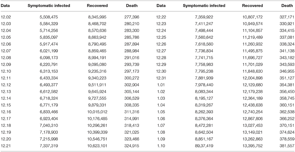
Table 2. Validation set for verifying the accuracy of the model.

The red curves are from February 22, 2020 to December 1, 2020, a total of 284 days, and the black curve is the simulation result of the model, as shown in Figure 3. We use the following equation to calculate the accuracy of model prediction:

$\begin{array}{ll}accuracyrate=\left(1-\frac{1}{n}·\frac{{\displaystyle \sum _{i=1}^n}|x_i-y_i|}{x_i}\right)\times 100\%& (7)\end{array}$

where x_i is the real value, y_i is the forecasting value, and n is the number of all data that needs to be forecast.

FIGURE 3

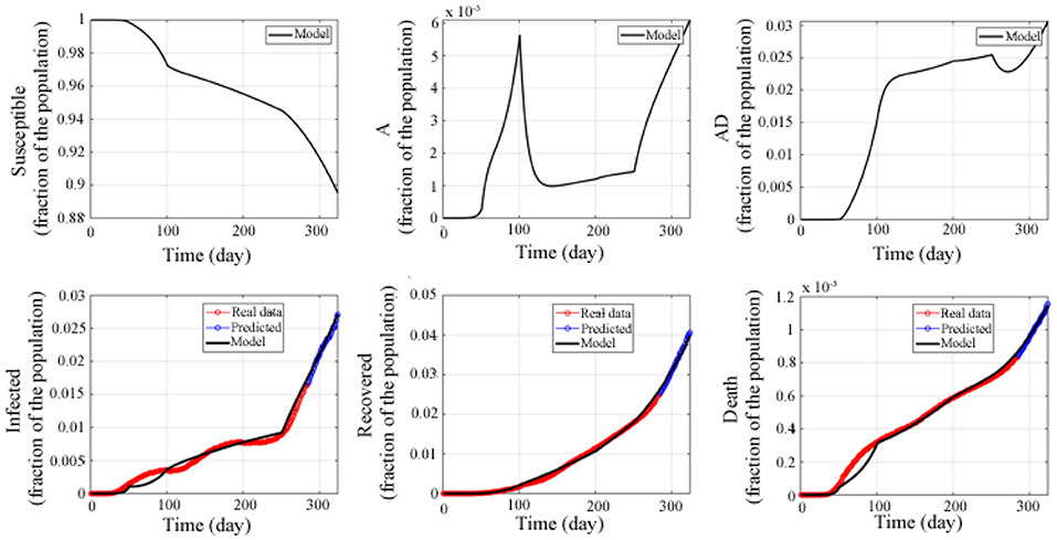
Figure 3. Fitted and predicted epidemic evolution. Epidemic evolution predicted by the model based on the available data about the COVID-19 outbreak in the United States.

The results show that the prediction accuracy rate of the current infected population I(t) is 98.33%, the prediction accuracy rate of the recovered population R(t) is 98.2%, and the prediction accuracy rate of the death population D(t) is 98.96%. This indicates that the model established in this study has high accuracy, and that the model can accurately predict the trend of the epidemic in the United States, and provides a guarantee for the following applied research.

Therefore, without taking into account the vaccine and the recovery of the survivors, we used the above model to make a long-term prediction of the epidemic in the United States (as shown in Figure 4). The prediction results showed that the susceptible population continued to decline, reaching the lowest level around the 1,560th day (4.45% of the total population) and continued until the end. The asymptomatic undiagnosed population reached a peak on the 518th day (1.53% of the total population), and then gradually decreased, dropping to 0% on the 1367th day. The asymptomatic diagnosed population reached the peak on the 570th day (10.32% of the total number), and gradually decreased, and the dropped to 0% on the 1,440th day. The infected population reached a peak around the 679th day (17.92% of the total number), gradually decreased, and then dropped to 0% around the 1,852th day. The number of recovered people was increasing, reaching a peak around the 1,533th day (91.87% of the total number), and was stable at this value. The number of deaths also increased gradually, reaching a peak around the 1,619th day (3.16% of the total number), and remained stable.

FIGURE 4

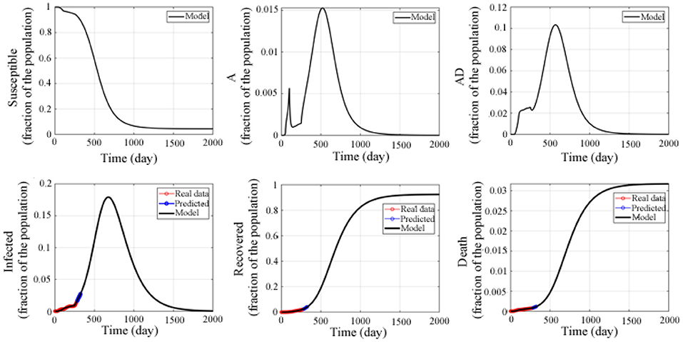
Figure 4. Predicted epidemic evolution for 2,000 days. Epidemic evolution predicted by the model based on the available data about the COVID-19 outbreak in the United States.

In addition, the attack rate was also studied and shown in Figure 5. The numerical simulation result indicated that the attacked individuals increased from the beginning and reached a peak around the 624th day, and that the maximum attack rate was 0.281, which is different from the asymptomatic and undetected, the asymptomatic and detected, and the symptomatic and infected.

FIGURE 5

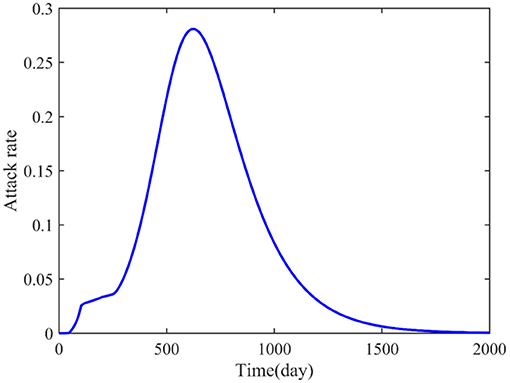
Figure 5. Predicted attack rate for 2,000 days.

Parameter Sensitivity Analysis

Next, parameter sensitivity analysis was performed to screen the factors that significantly affected the development of the epidemic. In order to overcome the influence of coupling between parameters on the results, we adopted a robust, highly calculated, and low-sample required global sensitivity analysis method, the Extended Fourier Amplitude Sensitivity Test (EFAST) method.

Based on the method of global sensitivity analysis, we obtained the first-order and full-order sensitivity indexes of 10 parameters in the mathematical model (Table 3 and Figures 6A,B). Based on reference, the sensitivity value (S_Ti) higher than 0.5 was defined as a sensitive parameter; otherwise, it was defined as a non-sensitive parameter (26).

TABLE 3

Table 3. First-order and full-order sensitivity indexes of the 10 parameters.

FIGURE 6

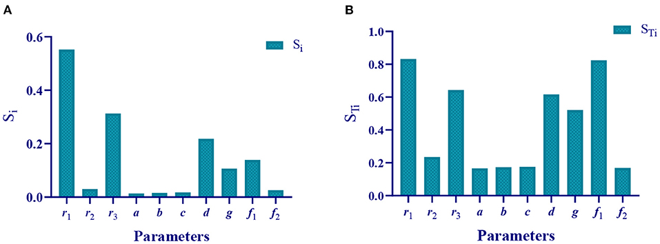
Figure 6. Sensitivity indexes of the 10 parameters. (A) First-order sensitivity index of the 10 parameters. (B) Full-order sensitivity index of the 10 parameters.

Therefore, we theoretically analyzed the parameters that affect the epidemic. The sensitivity parameters are r₁ = 0.8317 (the infection rate of asymptomatic undiagnosed population to susceptible population), r₃ = 0.6427 (the infection rate of symptomatic infection population to susceptible population), d = 0.6163 (probability of asymptomatically diagnosed population turning into symptomatically infected population), g = 0.521 (recovered rate of asymptomatic diagnosed population), and f₁ = 0.8247 (recovered rate of symptomatically infected population), non-sensitive parameters are r₂ = 0.2353 (the infection rate of the asymptomatic diagnosed population to the susceptible population), a = 0.1664 (the probability of the asymptomatic undiagnosed population becoming asymptomatic diagnosed population), b = 0.1731 (the probability of asymptomatic undiagnosed population becoming symptomatically infected), c = 0.1757 (the recovered rate of asymptomatic undiagnosed population), and f₂ = 0.169 (the death rate of symptomatic infection).

Verified Results of Parameter Sensitivity Analysis by Numerical Simulation

In the following, we used numerical simulation method to verify the correctness of the above global sensitivity analysis results. That is, the gradient change of parameters is used to study the impact of the output results of the susceptible population, the asymptomatic undiagnosed population, the asymptomatic diagnosed population, the symptomatic infected population, the recovered population, and the death population. For example, the initial value of parameter r₁ is 0.05, and it increases to 0.1 in steps of 0.01 to study the dynamics trend of each type of population.

Numerical simulation results showed that when parameter r₁ increases from 0.05 to 0.1 in steps of 0.01, the number of susceptible populations is greatly reduced, and that the number of asymptomatic undiagnosed population, asymptomatic diagnosed population, symptomatic infected population, recovered population, and death population all increases significantly with increase in r₁ (as shown in Supplementary Figure 1). This is consistent with the sensitivity of r₁, calculated by our theory, of 0.8317 (Table 3). Therefore, the parameter r₁ is a sensitive parameter that affects the epidemic.

When parameter r₂ increases from 0.0013 to 0.0018 in steps of 0.0001, the number of susceptible people, asymptomatic undiagnosed population, asymptomatic diagnosed population, symptomatic infected population, recovered population, and death population has no significant changes (Supplementary Figure 2). This is consistent with the sensitivity of parameter r₂ of 0.2353 (Table 3), indicating that parameter r₂ is an insensitive parameter, and that the change in parameter r₂ has no significant effect on the epidemic.

When parameter r₃ increased from 0.016 to 0.021 in steps of 0.001, the number of susceptible populations significantly reduced, and the number of asymptomatic undiagnosed population, asymptomatic diagnosed population, symptomatic infected population, recovered population, and death population all increased significantly with the increase in r₃ (Supplementary Figure 3). This is consistent with the sensitivity of r₃ of.6427 (Table 3). Therefore, parameter r₃ is a sensitive parameter that affects the epidemic. The sensitivity of parameter r₃ (0.6427) is lower than that of parameter r₃ (0.8317). The numerical simulation results also verify that the change in parameter r₁ has a greater impact on the epidemic than parameter r₃, which preliminarily proves that the parameter sensitivity obtained by our theoretical calculation is correct.

When parameter a increased from 0.13 to 0.18 in steps of 0.01, except for a certain degree of change in the asymptomatic undiagnosed population, the number of susceptible people, asymptomatic diagnosed population, symptomatic infected population, recovered population, and death population did not change significantly (Supplementary Figure 4), which is consistent with the sensitivity of parameter a of 0.1664 (Table 3), indicating that the parameter is a non-sensitive parameter with no significant impact on the epidemic.

When parameter b increased from 0.004 to 0.014 in steps of 0.002, the number of susceptible people, asymptomatic undiagnosed population, asymptomatic diagnosed population, symptomatic infected population, recovered population, and death population had no significant changes (Supplementary Figure 5), indicating that parameter b is a non-sensitive parameter, which is consistent with the sensitivity of parameter b of 1731 (Table 3).

Similarly, when parameter c increased from 0.005 to 0.01 in steps of 0.001, there was no significant change in the 6 groups of people (as shown in Supplementary Figure 6), indicating that parameter c is a non-sensitive parameter, which corresponds to the sensitivity of parameter c of 0.1757 (Table 3).

When parameter d increased from 0.013 to 0.018 in steps of 0.001, there were significant changes in the asymptomatic undiagnosed population, symptomatic infected population, and death population (Supplementary Figure 7), indicating that parameter d is a sensitive parameter, which is consistent with the sensitivity of parameter d of 0.6163 (Table 3).

When parameter g increased from 0.004 to 0.009 in steps of 0.001, in addition to the cured population, the number of susceptible populations, asymptomatic undiagnosed populations, asymptomatic diagnosed populations, symptomatic infected populations, and death populations all changed significantly (Supplementary Figure 8). It means that parameter g is a sensitive parameter that affects the epidemic, which is consistent with the sensitivity of parameter g of 0.521 (Table 3).

When parameter f₁ increased from 0.006 to 0.011 in steps of 0.001, the number of susceptible populations, asymptomatic undiagnosed population, asymptomatic diagnosed population, symptomatic infected population, and death population all changed significantly, except for the recovered. Besides, the amplitude of change is greater than the parameters d and g (Supplementary Figure 9). This is because the sensitivity of parameter f₁ is 0.8247, which is significantly greater than the sensitivity of parameters d and g (0.6163 and 0.521) (Table 3).

When parameter f₂ increased from 0.0002 to 0.0007 in steps of.0001, except for the obvious changes in death population, there was no significant change in the susceptible population, asymptomatic undiagnosed population, asymptomatic diagnosed population, symptomatic infected population, and recovered population (Supplementary Figure 10), indicating that parameter f₂ is a non-sensitive parameter, which is consistent with the sensitivity of parameter f₂ (0.169) (Table 3).

In summary, we have verified the sensitivity indexes of the 10 parameters obtained by theoretical calculations through numerical simulation. The results showed that gradient change in the sensitive parameters can significantly affect the development of the epidemic, and that change in the insensitive parameters has little impact on the epidemic (only a small impact on a certain group of people or no significant impact at all). Thus, the accuracy of the parameter sensitivity analysis was proved. In addition, the higher the sensitivity of the parameter, the greater the impact of parameter changes on the epidemic.

Influence of Parameter Changes on Attack Rate

In addition, the influence of parameter changes on attack rate was also studied. The simulation results (Figure 7A) showed that when increase parameter r1 from 0.05 to 0.1 in steps of 0.01, the attack rate increases significantly. which was shown in Figure 7A, where the color and black arrow have the same meaning as above. Similarly, increase r₃ from 0.016 to 0.021 in steps of 0.001 (Figure 7C), increase g from 0.004 to 0.009 in steps of 0.001 (Figure 7H), and increase f₁ from 0.006 to 0.011 in steps of 0.001 (Figure 7I), the attack rates are all affected significantly. What the difference is that with the increase in r₁ and r₃, the attack rate also increases, and when parameters g and f₁ increase, the attack rate decreases significantly. This is consistent with our sensitive analysis.

FIGURE 7

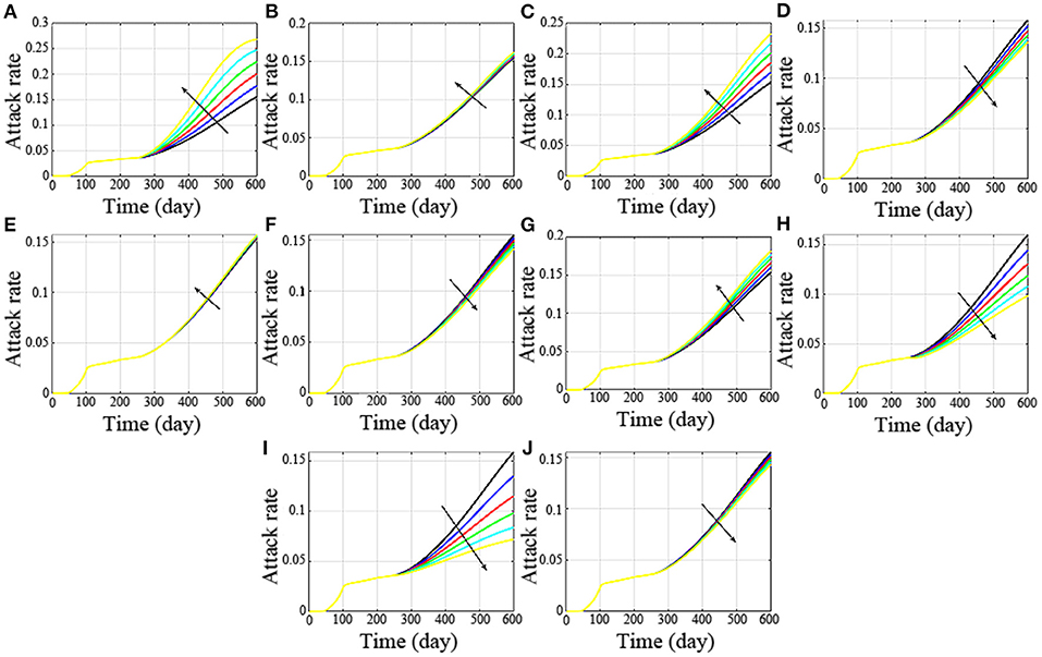
Figure 7. Influence of parameter changes on attack rate. (A-J) are the attack rates with the changes of the parameter r₁, r₂, r₃, a, b, c, d, g, f₁ and f₂, respectively.

Besides, if r₂ increases from 0.0013 to 0.0018 in steps of 0.0001, the attack rate has no significant difference (Figure 7B). Similarly, increase a from 0.13 to 0.14, 0.15, 0.16, 0.17 and 0.18 (Figure 7D), increase parameter b from 0.004 to 0.006, 0.008, 0.01, 0.012, and 0.014 (Figure 7E), increase parameter c from 0.005 to 0.006, 0.007, 0.008, 0.009, and 0.01 (Figure 7F), there was no significant change in their attack rates. The non-sensitive parameters are consistent with our theoretical analysis.

However, when d increases from 0.013 to 0.018 in steps of 0.001, the change is not particularly dramatic. This is because with the increase in d, the asymptomatic undiagnosed population and symptomatic infected population increased, and the asymptomatic diagnosed population decreased.

Conclusion

Based on the transmission characteristics of COVID-19 in the population, in this study, the population was divided into 6 categories, namely, the susceptible population, asymptomatic undiagnosed population, asymptomatic diagnosed population, symptomatic infected population, recovered population, and death population, and a differential mathematical model was established to describe and predict the trend of COVID-19. Based on the real-time big data report of Baidu's epidemic situation (https://voice.baidu.com/act/newpneumonia/newpneumonia?), the number of the currently infected with COVID-19, recovered, and death from February 22, 2020 to December 1, 2020 in the United States was collected. The NLS algorithm was used to estimate the model parameters, and the correlations were calculated between the mathematical model and the collected epidemic data (the correlation between the number of the currently infected simulated by the mathematical model, and the collected infected is 98.85%, the correlation between the cured number simulated by the mathematical model and the collected cured number is 99.84%, and the correlation between the death simulated by the mathematical model and the collected death is 99.54%). Besides, we also calculated the basic reproductive number of each stage to access the transmission capacity. Subsequently, we continued to collect data (the number of the current infected, recovered and death of COVID-19 in the United States from December 2, 2020 to January 10, 2021, and verified the accuracy of the model. The results show that the prediction accuracy of the infected I(t) is 98.33%, the recovered R(t) is 98.2%, and the death D(t) is 98.96%. Therefore, this model can effectively describe and predict the evolution of the epidemic in the United States.

In order to overcome the influence of coupling effect between parameters on the results, the global sensitivity analysis method was adopted to analyze the sensitivity of the parameters, so as to obtain the sensitive parameters that affected the evolution of the epidemic, and provide effective control strategies for the prevention and control of the epidemic by adjusting the sensitive parameters.

The global sensitivity analysis results show that parameters r₁ (S_Ti = 0.8317), r₃ (S_Ti = 0.6427), d (S_Ti = 0.6163), g (S_Ti = 0.521), and f₁(S_Ti = 0.8247) are sensitive parameters, and that parameters r₂ (S_Ti = 0.2353), a (S_Ti = 0.1664), b (S_Ti = 0.1731), c (S_Ti = 0.1757), and f₂ (S_Ti = 0.169) are non-sensitive parameters. Next, the method of parameter gradient change is adopted to verify the correctness of the parameter sensitivity results of the theoretical analysis. The results showed that change in the sensitive parameters could significantly affect change in the epidemic, and that change in the insensitive parameters had no significant impact on the epidemic. For example, the sensitivity of parameter r1 is S_Ti = 0.8317. When r₁ increases from 0.05 to 0.1 in steps of 0.01, the number of the susceptible reduced greatly, while the asymptomatic undiagnosed, asymptomatic diagnosed, symptomatic infected, recovered, and death all increased significantly with the increase in r₁. The sensitivity of parameter r₂ is S_Ti = 0.2353. When r₂ increases from 0.0013 to 0.0018 in steps of 0.0001, the number of the susceptible, asymptomatic undiagnosed, asymptomatic diagnosed, symptomatic infected, recovered, and death has no significant change.

Therefore, based on the above sensitivity analysis results, this study proposes the following control strategies:

1. Strengthen isolation. Because strengthening isolation can effectively reduce the infection rate of the asymptomatic undiagnosed to the susceptible (r₁) and the infection rate of the symptomatic infected to the susceptible (r₃). Reducing r₁ and r₃ can increase the number of the susceptible, and decrease the number of the asymptomatic undiagnosed, asymptomatic diagnosed, symptomatic infected, and death. In addition, if someone has to travel, wearing a mask may also be an effective isolation measure.

2. Strengthen the monitoring and treatment of the asymptomatic diagnosed. When the probability (d) that the asymptomatic diagnosed turns into the symptomatic infected increases, the number of the susceptible population will decrease, but the number the asymptomatic undiagnosed, symptomatic infected, and death will significantly increase. In addition, the recovered rate (g) of the asymptomatic diagnosed should be increased, because when parameter g increases, the number of the susceptible increases, while the number of the asymptomatic undiagnosed, asymptomatic diagnosed, symptomatic infected, and death increases significantly with the increase in g.

3. Improve the recovered rate of the symptomatic infected. When the recovered rate (f₁) of the symptomatic infected increases, the number of the susceptible will increase, while the number of the asymptomatic undiagnosed, asymptomatic diagnosed, symptomatic infected and death will decrease significantly.

Data Availability Statement

The original contributions presented in the study are included in the article/Supplementary Material, further inquiries can be directed to the corresponding author/s.

Author Contributions

DS: conceptualization, methodology, software, funding acquisition, formal analysis, resources, investigation, writing-original draft, supervision, and writing-review editing. XL: data curation and project administration. JL: simulations, supervision and funding support. All authors contributed to the article and approved the submitted version.

Funding

This study was supported by the National Natural Science of China under Grant Nos. 62103287 and 62003071. This study was also supported by Shenzhen Institutes of Advanced Technology Innovation Program for Excellent Young Researchers (RCBS20200714114856171).

Conflict of Interest

The authors declare that the research was conducted in the absence of any commercial or financial relationships that could be construed as a potential conflict of interest.

Publisher's Note

All claims expressed in this article are solely those of the authors and do not necessarily represent those of their affiliated organizations, or those of the publisher, the editors and the reviewers. Any product that may be evaluated in this article, or claim that may be made by its manufacturer, is not guaranteed or endorsed by the publisher.

Acknowledgments

The authors would like to thank the editor and the reviewers for their valuable suggestions.

Supplementary Material

The Supplementary Material for this article can be found online at: https://www.frontiersin.org/articles/10.3389/fpubh.2021.751940/full#supplementary-material

References

1. Coronavirus disease 2019. Available online at: https://en.wikipedia.iwiki.eu.org/wiki/Coronavirus_disease_2019

2. Centers for Disease Control and Prevention. Available online at: https://www.cdc.gov/coronavirus/2019-ncov/transmission/variant.html

3. González-Parra G, Arenas AJ, Chen-Charpentier BM, Rivera J. A fractional order epidemicmodel for the simulation of outbreaks of influenza A(H1N1). Math Meth Appl Sci. (2014) 37:2218–26. doi: 10.1002/mma.2968

PubMed Abstract | CrossRef Full Text | Google Scholar

4. Elaiw AM, AlShamrani NH. Global stability of humoral immunity virus dynamics models with nonlinear infection rate and removal. Nonlinear Analysis. (2015) 26:161–90. doi: 10.1016/j.nonrwa.2015.05.007

CrossRef Full Text | Google Scholar

5. Sms A, Pgd A. A fractional order differential equation model for hepatitis B virus with saturated incidence. Res Phys. (2021) 24:104114. doi: 10.1016/j.rinp.2021.104114

CrossRef Full Text | Google Scholar

6. Gao F, Li X, Li W, Zhou X. Stability analysis of a fractional-order novel hepatitis B virus model with immune delay based on Caputo-Fabrizio derivative. Chaos Solitons Fractals. (2021) 142:110436. doi: 10.1016/j.chaos.2020.110436

CrossRef Full Text | Google Scholar

7. Kucharski AJ, Russell TW, Diamond C, Liu Y, Edmunds J, Funk S, et al. Early dynamics of transmission and control of COVID-19: a mathematical modelling study. Lancet Infect Dis. (2020) 20:553–8. doi: 10.1016/S1473-3099(20)30144-4

PubMed Abstract | CrossRef Full Text | Google Scholar

8. Wu JT, Leung K, Leung GM. Nowcasting and forecasting the potential domestic and international spread of the 2019-nCoV outbreak originating in Wuhan, China: a modelling study. Lancet. (2020) 395:689–97. doi: 10.1016/S0140-6736(20)30260-9

PubMed Abstract | CrossRef Full Text | Google Scholar

9. Nisar KS, Ahmad S, Ullah A, Shah K, Alrabaiah H, Arfan M. Mathematical analysis of SIRD model of COVID-19 with Caputo fractional derivative based on real data. Res Phys. (2021) 21:103772. doi: 10.1016/j.rinp.2020.103772

PubMed Abstract | CrossRef Full Text | Google Scholar

10. Zhu H, Li Y, Jin X, Huang J, Liu X, Qian Y, et al. Transmission dynamics and control methodology of COVID-19: A modeling study. Appl Math Model. (2021) 89:1983–98. doi: 10.1016/j.apm.2020.08.056

PubMed Abstract | CrossRef Full Text | Google Scholar

11. Demongeot J, Griette Q, Magal P. SI epidemic model applied to COVID-19 data in mainland China. R Soc Open Sci. (2020) 7:201878. doi: 10.1098/rsos.201878

PubMed Abstract | CrossRef Full Text | Google Scholar

12. Huang Q, Kang YS. Mathematical modeling of COVID-19 control and prevention based on immigration population data in China: model development and validation. JMIR Public Health Surveill. (2020) 6:e18638. doi: 10.2196/18638

PubMed Abstract | CrossRef Full Text | Google Scholar

13. Reiner RC, Barber RM, Collins JK, Zheng P, Adolph C, Albright J, et al. Modeling COVID-19 scenarios for the United States. Nat Med. (2021) 27:94–105. doi: 10.1038/s41591-020-1132-9

PubMed Abstract | CrossRef Full Text | Google Scholar

14. Oliveira JF, Jorge DCP, Veiga RV, Rodrigues MS, Torquato MF, da Silva NB, et al. Mathematical modeling of COVID-19 in 14.8 million individuals in Bahia, Brazil. Nat Commun. (2021) 12:333–45. doi: 10.1038/s41467-020-19798-3

PubMed Abstract | CrossRef Full Text | Google Scholar

15. Kyrychko YN, Blyuss KB, Brovchenko I. Mathematical modelling of the dynamics and containment of COVID-19 in Ukraine. Sci Rep. (2020) 10:19662. doi: 10.1038/s41598-020-76710-1

PubMed Abstract | CrossRef Full Text | Google Scholar

16. Giordano G, Blanchini F, Bruno R, Colaneri P, Colaneri M. Modelling the COVID-19 epidemic and implementation of population-wide interventions in Italy. Nat Med. (2020) 2020:1–6. doi: 10.1038/s41591-020-0883-7

PubMed Abstract | CrossRef Full Text | Google Scholar

17. Chang SL, Harding N, Zachreson C, Cliff OM, Prokopenko M. Modelling transmission and control of the COVID-19 pandemic in Australia. Nat Commun. (2020) 11:5710–22. doi: 10.1038/s41467-020-19393-6

PubMed Abstract | CrossRef Full Text | Google Scholar

18. Annas S, Isbar Pratama M, Rifandi M, Sanusi W, Side S. Stability analysis and numerical simulation of SEIR model for pandemic COVID-19 spread in Indonesia. Chaos Solitons Fractals. (2020) 139:110072. doi: 10.1016/j.chaos.2020.110072

PubMed Abstract | CrossRef Full Text | Google Scholar

19. Jahanshahi H, Munoz-Pacheco JM, Bekiros S, Alotaibi ND. A fractional-order SIRD model with time-dependent memory indexes for encompassing the multi-fractional characteristics of the COVID-19. Chaos Solitons Fractals. (2021) 143:110632. doi: 10.1016/j.chaos.2020.110632

PubMed Abstract | CrossRef Full Text | Google Scholar

20. Davies NG, Barnard RC, Jarvis CI, Russell TW, Semple MG, Jit M, et al. Association of tiered restrictions and a second lockdown with COVID-19 deaths and hospital admissions in England: a modelling study. Lancet Infect Dis. (2020) 21:482–92. doi: 10.1016/S1473-3099(20)30984-1

PubMed Abstract | CrossRef Full Text | Google Scholar

21. Català M, Alonso S, Alvarez-Lacalle E, López D, Cardona P-J, Prats C. Empirical model for short-time prediction of COVID-19 spreading. PLoS Comput Biol. (2020) 16:e1008431. doi: 10.1371/journal.pcbi.1008431

PubMed Abstract | CrossRef Full Text | Google Scholar

22. Hasan A, Putri ERM, Susanto H, Nuraini N. Data-driven modeling and forecasting of COVID-19 outbreak for public policy making. ISA Transactions. (2021) 138:1–10. doi: 10.1016/j.isatra.2021.01.028

PubMed Abstract | CrossRef Full Text | Google Scholar

23. Firth JA, Hellewell J, Klepac P, Kissler S, Jit M, Atkins KE, et al. Using a real-world network to model localized COVID-19 control strategies. Nat Med. (2020) 26:1616–22. doi: 10.1038/s41591-020-1036-8

PubMed Abstract | CrossRef Full Text | Google Scholar

24. Li M, Zu J. The review of differential equation models of HBV infection dynamics. J Virol Methods. (2019) 266:103–13. doi: 10.1016/j.jviromet.2019.01.014

PubMed Abstract | CrossRef Full Text | Google Scholar

25. Alahdal M, Sun D, Duan L, Ouyang H, Wang M, Xiong J, et al. Forecasting sensitive targets of the kynurenine pathway in pancreatic adenocarcinoma using mathematical modeling. Cancer Sci. (2021) 112:1481–94. doi: 10.1111/cas.14832

PubMed Abstract | CrossRef Full Text | Google Scholar

26. Cannavo F. Sensitivity analysis for volcanic source modeling quality assessment and model selection. Comp Geosci. (2012) 44:52–9. doi: 10.1016/j.cageo.2012.03.008

CrossRef Full Text | Google Scholar

27. Xw A, Zhen WA, Jx B. Stability and bifurcation control of a delayed fractional-order eco-epidemiological model with incommensurate orders. J Franklin Institute. (2019) 356:8278–95. doi: 10.1016/j.jfranklin.2019.07.028

CrossRef Full Text | Google Scholar