Construction and validation of tertiary models for predicting growth of Salmonella Infantis in chicken liver during a processing chain deviation

Salmonella Infantis is a top human clinical isolate that is found at low levels in chicken liver after primary processing. However, temperature abuse of chicken liver during secondary processing can lead to growth of Salmonella and higher risk of salmonellosis. Therefore, a three-phase linear, polynomial regression, tertiary model (TM_PR) and a multiple layer feedforward neural network with two nodes in the hidden layer, tertiary model (TM_NN) for growth of Salmonella Infantis in chicken liver as a function of dose (10¹–10⁶), time (0–8 h), and temperature (18–30°C) were constructed, validated, and compared using the criteria of the Acceptable Prediction Zones (APZ) method. When the proportion of residuals in the APZ or pAPZ was ≥0.7, predictions were considered acceptable. The pAPZ for the dependent data (n = 360) was 0.979 for the TM_PR and 0.976 for the TM_NN, whereas the pAPZ for the independent data for interpolation (n = 72) was 0.968 for the TM_PR and 0.964 for the TM_NN. Thus, both the TM_PR and TM_NN were validated for interpolation, had similar performance, and can be used with confidence to predict the growth of Salmonella Infantis in chicken liver during a secondary processing deviation of temperature abuse. However, construction of the TM_PR involved three steps, whereas construction of the TM_NN involved one step. Thus, the TM_NN was easier to construct and validate. Nonetheless, the final TM included the TM_PR and TM_NN because the TM_PR predicted lag time and growth rate, whereas the TM_NN did not.

1 Introduction

Salmonella can colonize the liver of live chickens before primary processing (Khan et al., 2024; Wang et al., 2024; Yokoyama et al., 2015). In addition, Salmonella in water, on equipment, or on hands can cross-contaminate chicken liver during primary processing (Rivera-Perez et al., 2014). Thus, chicken liver can be contaminated with Salmonella before secondary processing of it into other products like chicken liver paté (Jung et al., 2019; Porto-Fett et al., 2019; Procura et al., 2019).

Chicken liver is high in nutrients and has a pH and water activity that supports the growth of Salmonella at temperatures encountered during secondary processing in the processing plant or restaurant, institution, or home kitchen (Bovill et al., 2000). Therefore, secondary processing of chicken livers can provide an opportunity for Salmonella to grow to levels that pose a higher risk of salmonellosis (Hanson et al., 2014; Lanier et al., 2018). Models that predict the growth of Salmonella in chicken liver are valuable tools for assessing the impact of processing deviations on the risk of salmonellosis from chicken liver. However, there are currently no models for the growth of Salmonella in chicken liver.

A three step method for developing tertiary models (TM) for growth of Salmonella in food using regression methods is shown in Figure 1 (Whiting, 1995). In step one, data for log number of Salmonella in food over time for one combination of independent variables is fitted to a primary model (PM), like the three phase linear (3PL) model of Buchanan et al. (1997). The PM_3PL has parameters for initial log number (Y1), lag time (X1), time to final log number (X2), and final log number (Y2). In step two, a dataset of the PM parameters and combinations of independent variables investigated is fitted to a secondary model (SM) like the polynomial regression (PR) model of Thayer et al. (1987). In step three, the SM are incorporated back into the PM to construct a TM that predicts the log number of Salmonella in the food over time as a function of the independent variables. Once constructed, the next step is to validate the TM.

Figure 1

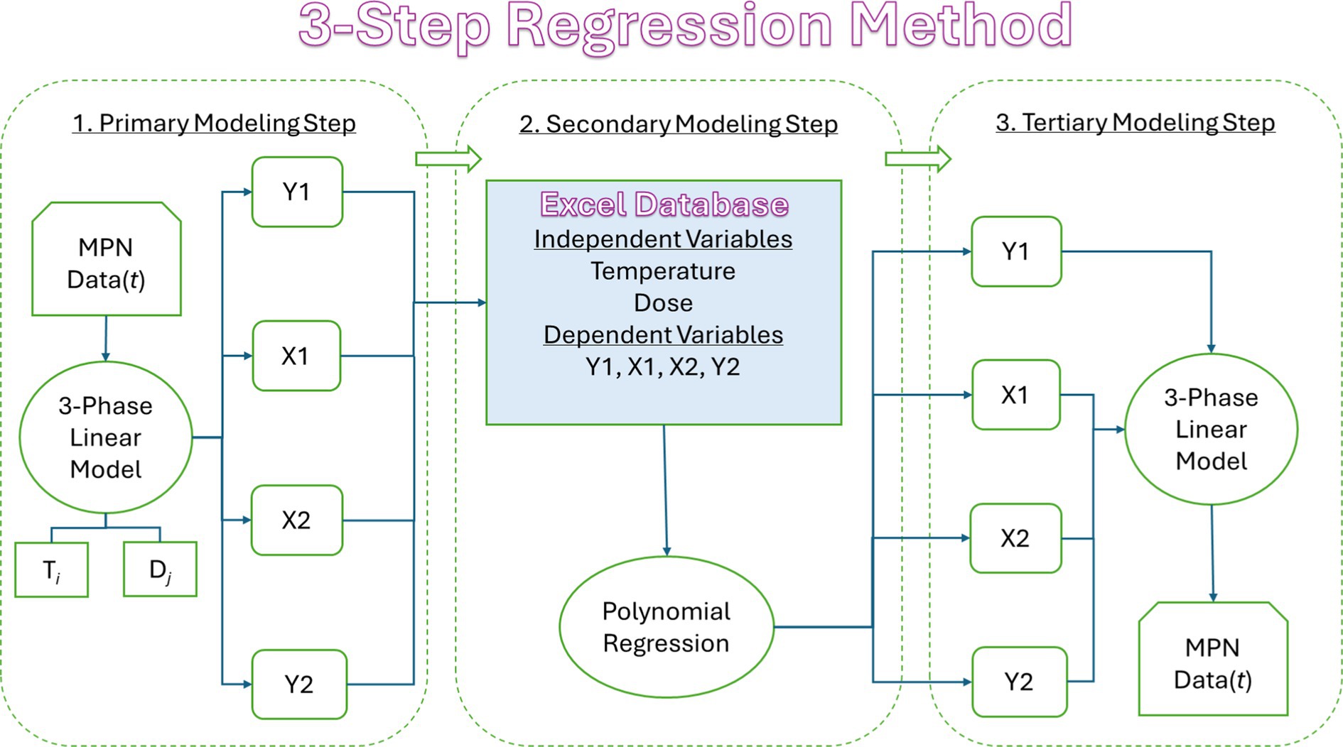
Figure 1. Flow diagram showing the three steps of the process used to construct a tertiary model using regression methods. MPN, most probable number; t, time; T, temperature; D, dose; Y1, initial MPN; X1, lag time; X2, time to final MPN; and Y2, final MPN.

Model validation occurs in three steps (Figure 2). In step one, model predictions are compared to dependent data. In step two, model predictions are compared to independent data for interpolation. In step three, model predictions are compared to independent data for extrapolation. Model validation occurs when all criteria for test data, model performance, and model validation are met for the first two steps. The third step is optional but important because validation of a model to a new independent variable can save time and money by identifying conditions for which new models are not needed. In the present study, the test data, model performance, and model validation criteria of the Acceptable Prediction Zones (APZ) method (Oscar, 2020b, 2023) were used to validate PM, SM, and TM.

Figure 2

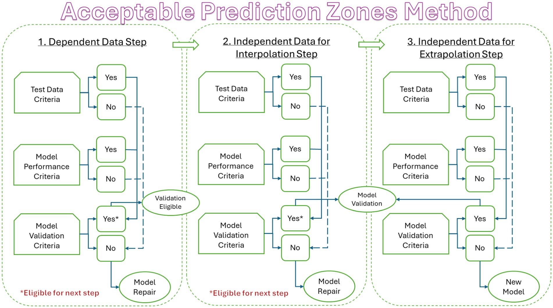
Figure 2. Flow diagram showing the three steps of the model validation process used in the Acceptable Prediction Zones method in the Validation Software Tool (ValT) for predictive microbiology.

The three-step methods for construction and validation of models for growth of Salmonella in food are time consuming and complex. However, it is possible to construct the TM in one step using a neural network (NN) method (Oscar, 2009, 2015, 2018). Therefore, the current study was undertaken to construct, validate, and compare, for the first time, a TM_PR to a TM_NN for growth of Salmonella Infantis in chicken liver as a function of dose (10¹–10⁶), time (0–8 h), and temperature (18–30°C). The Salmonella serotype and dose range investigated and modeled were based on results of a previous study that determined Salmonella serotype prevalence and number in chicken liver (Oscar, 2021), whereas the time and temperature ranges investigated and modeled were based on those commonly encountered during the secondary processing of chicken livers in a processing plant or in a restaurant, institution, or home kitchen.

2 Methods

2.1 Experimental designs

The experiment for model construction was a replicated (n = 6), 3 × 5 × 4, full factorial of dose (10¹, 10^3.5, 10⁶), time (0, 2, 4, 6, 8 h), and temperature (18, 22, 26, 30°C), whereas the experiment for model validation for interpolation was a replicated (n = 3), 2 × 4 × 3 full factorial of dose (10^2.25, 10^4.75), time (1, 3, 5, 7 h), and temperature (20, 24, 28°C). The doses, times, and temperatures investigated and modeled were based on the following considerations. First, they were based on the ranges identified above. Second, they were based on the test data criterion of the APZ method for even spacing of independent variable values (Oscar, 2020b, 2023). Third, they were based on the test data criterion of the APZ method for intermediate independent variable values for internal validation of validation for interpolation.

2.2 Data collection

The method of Oscar (2024a) was used to collect the most probable number (MPN) data for model construction and validation with some modifications. A single brand of chicken liver rather than a single brand of ground turkey was used. Five doses instead of one dose of Salmonella Infantis were used. Storage trials were 8 h instead of 28 h and were conducted at 18–30°C instead of 16–40°C. Thus, the current model is for chicken liver instead of ground turkey, and the range of prediction is wider for dose and narrower for time and temperature.

2.3 Model construction

The method of Oscar (2024a) was used to construct the TM_PR with modifications. First, the PM_3PL was fitted to MPN data from individual storage trials instead of combined storage trials. Second, PR (StatTools, Decision Tools Suite, version 8.2, Lumivero) was used for SM instead of the SM of Oscar (2024a). Third, the TM_PR had three (dose, time, temperature) independent variables instead of two (time, temperature). The PR form was:

$\mathrm{Y}={\mathrm{B}}_0+{\mathrm{B}}_1\mathrm{D}+{\mathrm{B}}_2\mathrm{T}+{\mathrm{B}}_3{\mathrm{D}}^2+{\mathrm{B}}_4{\mathrm{T}}^2$

where Y was a PM_3PL parameter, B₀ to B₄ were regression coefficients, D was dose, and T was temperature. The PM_3PL parameters were X1 = lag time (h); Y1 = initial MPN (log₁₀/0.2 g); X2 = time to final MPN (h); and Y2 = final MPN (log₁₀/0.2 g). The TM_PR was constructed in Excel (Office 365, MicroSoft).

The method of Oscar (2020a), which uses the BestNet Search option of NeuralTools to identify the best-performing TM_NN, was used with one modification to construct a multiple layer feedforward neural network with two nodes in the hidden layer that had three (dose, time, temperature) instead of two (time, temperature) independent variables. Here, the dependent data (n = 360) were used to train the TM_NN, whereas the independent data for interpolation (n = 72) were used to test the TM_NN for generalization. The TM_NN was constructed in Excel with a spreadsheet add-in program (NeuralTools, Decision Tools Suite 8.2, Lumivero), which is needed to simulate the TM_NN.

2.4 Model validation

The TM_PR and TM_NN and the PM and SM were validated using the APZ method of Oscar (2023) in the Validation Software Tool (ValT) for predictive microbiology (Oscar, 2020b). In brief, the observed and predicted values for the dependent data and independent data for interpolation were entered into ValT followed by calculation of the pAPZ, which was the proportion of residuals in the partly and fully acceptable prediction zones. Next, the “yes” or “no” questions in the decision trees for dependent data and independent data for interpolation were answered and then ValT provided an objective “yes” or “no” decision about model validation. A model was validated when it satisfied all APZ criteria for dependent data and independent data for interpolation.

A model was considered to provide predictions with acceptable bias and accuracy when pAPZ was >0.7. The justification for this threshold and the boundaries of the partly and fully acceptable prediction zones for the different types of models is complex and thus, beyond the scope of this study, but can be found in previous studies (Oscar, 2005a, 2005b, 2020b, 2023).

2.5 Statistical analysis

Two-way, analysis of variance (ANOVA) in Prism for Windows (version 10, GraphPad Software, San Diego) was used to determine if lag time and growth rate were affected (p ≤ 0.05) by dose, temperature, or their interaction and to determine if prediction bias (mean residual) and prediction accuracy (mean absolute residual) were affected (p ≤ 0.05) by type of data, type of TM, or their interaction.

3 Results

3.1 Primary modeling and validation

3.1.1 Primary modeling of dependent data

Figure 3 shows typical fits of the PM_3PL to the growth curves. The rest of the growth curve fits are in Supplementary S42–S131 to provide a complete visual appraisal of data and model fit quality. The results in Figure 3 showed that curves had two and on rare occasions three phases of growth. Luckily, the PM_3PL could be fitted to curves with one, two, or three phases of growth as well as those with limited data in a growth phase (Figure 3) and still provide complete and reliable PM parameter data for SM and TM construction. This contrasts with other PM like the Gompertz, Baranyi, and Huang that require more complete data in all growth phases to generate reliable PM parameter data for SM and TM construction.

Figure 3

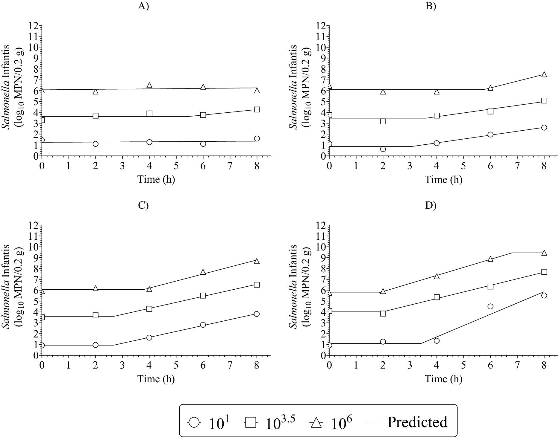
Figure 3. Typical growth curves fits of the three-phase linear primary model to the log₁₀ most probable number (MPN) data (dependent data) for growth of Salmonella Infantis in chicken liver as a function of dose (10¹, 10^3.5, 10⁶), time (0, 2, 4, 6, 8 h), and temperatures of (A) 18°C; (B) 22°C; (C) 26°C; and (D) 30°C. Results are from one storage trial per combination of independent variables.

3.1.2 Validation of the primary model (dependent data)

The APZ analysis in ValT for the PM_3PL and dependent data (n = 360) is shown in Figure 4. Here, answers to questions (Q) 1–3 for test data in the decision tree were “yes” meaning that the criteria were met and where answers of “yes” lead to model validation, whereas and a single answer of “no” leads to model repair (Figure 2). Thus, the data were used in model construction, the levels of the independent variables (dose, time, temperature) were evenly spaced, and there was a minimum of four prediction cases (pair of observed and predicted values) for each combination of independent variables.

Figure 4

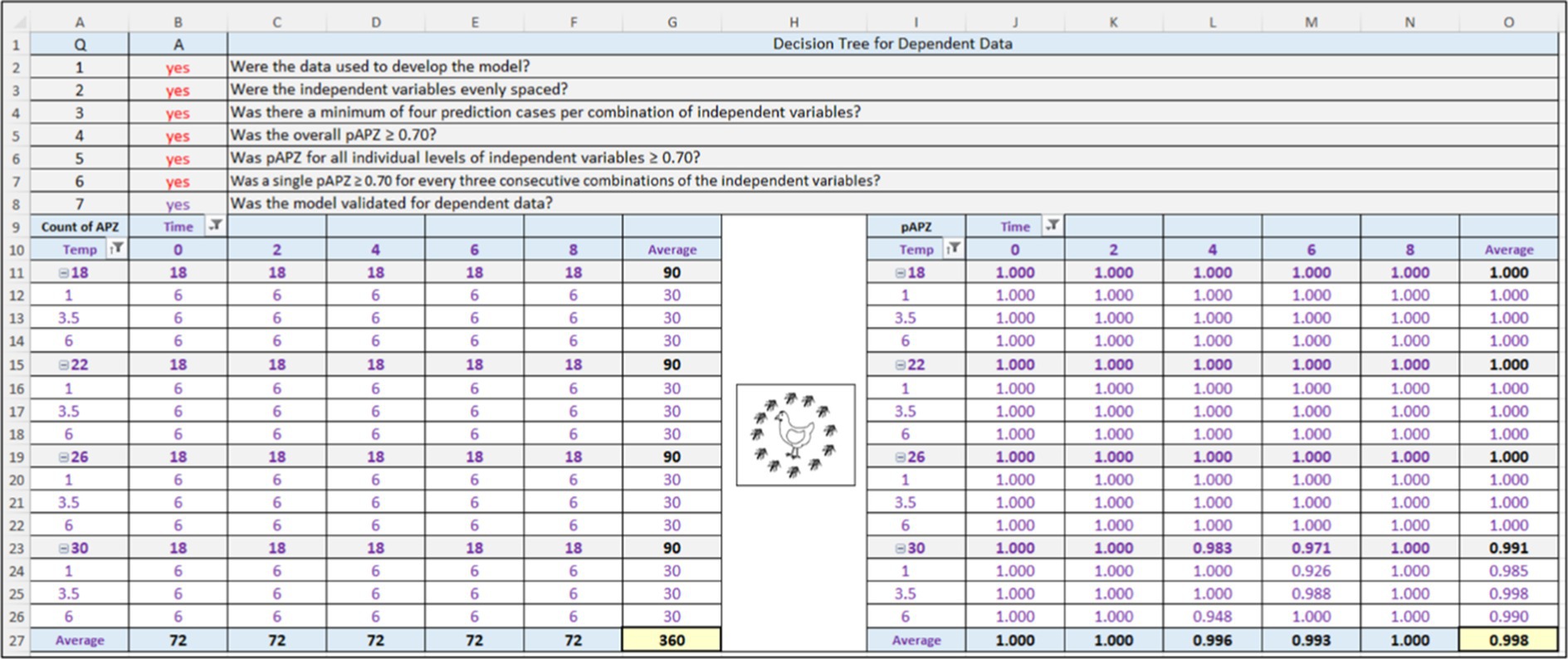
Figure 4. Screenshot of the Acceptable Prediction Zones (APZ) analysis in the Validation Software Tool for the three-phase linear, primary model that predicts the growth of Salmonella Infantis in chicken liver over time for individual combinations of dose (10¹, 10^3.5, or 10⁶) and temperature (18, 22, 26, or 30°C). Results are for the dependent data.

Continuing with the validation (Figure 4), answers to Q4 to Q6 for model performance were “yes” indicating that the PM_3PL satisfied these criteria. In other words, the PM_3PL had no local or global prediction problems for the dependent data. Because the PM_3PL satisfied the criteria for test data and model performance, the response to Q7 for the model validation criterion, which was automatically provided by a formula in ValT, was “yes” indicating that the PM_3PL was validated for the dependent data or had acceptable goodness-of-fit.

The results in Figure 4 for the PM_3PL and dependent data were confirmed in Figure 5, which shows the distribution of residuals (observed–predicted) among the partly and fully acceptable prediction zones as a function of the independent variables of dose, time, and temperature. Most residuals (357 of 360) were in the fully acceptable prediction zone from −1.0 to 0.5 log₁₀ MPN per 0.2 g of chicken liver. The rest (3 of 360) were in the partly acceptable prediction zone from −1.0 to −2.0 log₁₀ MPN per 0.2 g of chicken liver, and from 0.5 to 1.0 log₁₀ MPN per 0.2 g of chicken liver. None of the residuals were outside the partly and fully acceptable prediction zones.

Figure 5

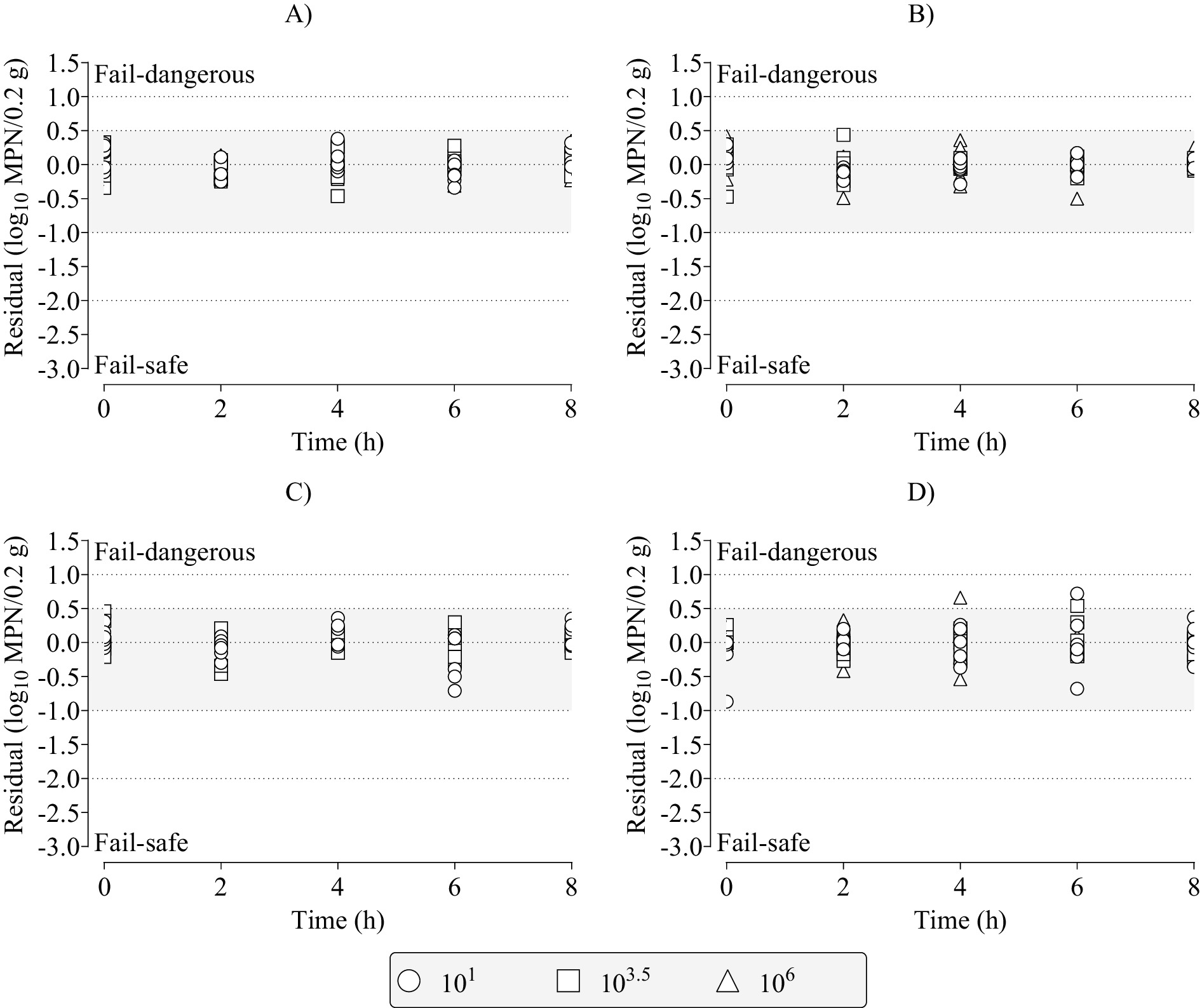
Figure 5. Distribution of residuals (observed–predicted) among the partly (dotted lines with no fill) and fully (dotted lines with gray fill) acceptable prediction zones for the three-phase linear, primary model fits to the dependent data for growth of Salmonella Infantis in chicken liver as a function of individual combinations of dose (10¹, 10^3.5, 10⁶), time (0, 2, 4, 6, 8 h), and temperatures of (A) 18°C; (B) 22°C; (C) 26°C; or (D) 30°C.

The results of the APZ analysis in ValT for the PM_3PL and dependent data are summarized in Table 1 (analysis A). The global pAPZ and the minimum pAPZ for a single level of independent variables, and a combination of all independent variables were all ≥0.926. In addition, the mean residual, a measure of prediction bias, and mean absolute residual, a measure of prediction accuracy, were close to zero. Together, these results indicated that the PM_3PL fitted the dependent data well.

Table 1

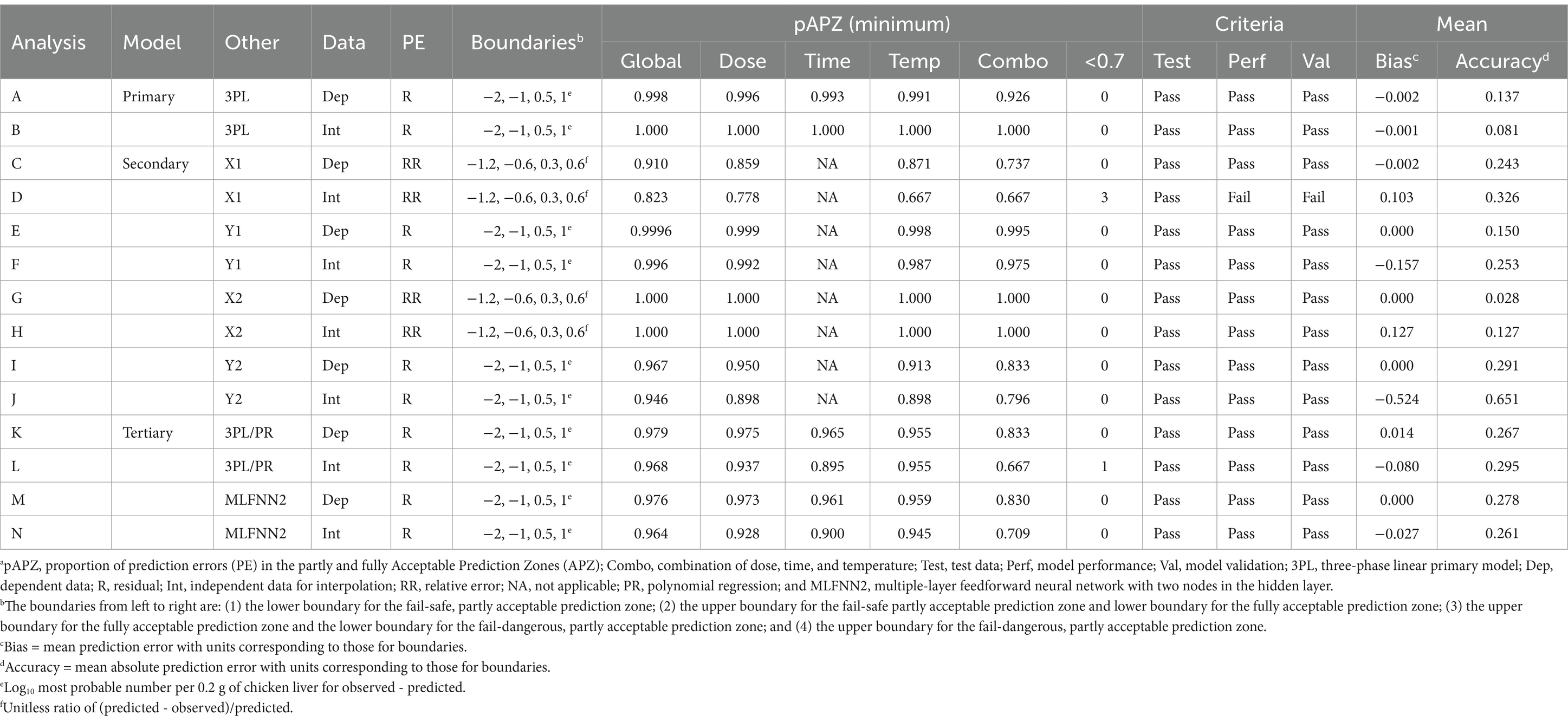
Table 1. Statistical summary of the acceptable prediction zones analysis of primary, secondary, and tertiary model performance for growth of Salmonella Infantis in chicken liver^a.

3.1.3 Primary modeling of the independent data for interpolation

The PM_3PL was fitted to the independent data for interpolation, which was necessary to obtain the PM parameter data needed to validate the SM. The robustness of the PM_3PL was important here because the growth curves in this set of data only had four sampling times (S6).

3.1.4 Validation of the primary model for the independent data for interpolation

The APZ analysis in ValT for the PM_3PL and independent data for interpolation is provided in S7 where the decision tree had nine questions. Questions 1 and 9 were for model validation criteria, Q2–Q5 were for test data criteria, and Q6–Q8 were for model performance criteria. Again, answers of “yes” led to model validation and a single answer of “no” led to model repair (Figure 2). A prerequisite was validation of the PM_3PL for dependent data or an automated answer of “yes” to Q1, which was the case here (S7).

The test data criteria Q2–Q6 ensured that the data were not used in model construction, that levels of independent variables were intermediate to those used in model construction, sufficiently replicated (n = 3 or more) so that an unbiased and accurate evaluation of model performance was obtained, and that the data were collected using the same methods as those used to collect the data for model construction so that the comparison of observed and predicted values was not confounded by differences in data collection methods. The answers to Q2–Q6 in the decision tree of S7 were “yes” indicating that the independent data for interpolation satisfied the APZ criteria for test data.

As shown in S8, all residuals (72 of 72) were in the fully acceptable prediction zone resulting in pAPZ of 1.00 for all combinations and levels of independent variables and overall (analysis B in Table 1). These results indicated that the PM_3PL fitted the independent data for interpolation well. Thus, the PM_3PL was a good choice.

3.2 Secondary modeling and validation

3.2.1 Statistical summary of the secondary modeling of the dependent data

Table 2 provides a statistical summary of the SM_PR fits to the PM parameter data. The R² value was moderate for X1, high for Y1, very low for X2, and high for Y2. Temperature had a nonlinear effect (p ≤ 0.05) on X1, no effect (p > 0.05) on Y1, a nonlinear effect (p ≤ 0.05) on X2, and no effect (p > 0.05) on Y2 (Table 2). Dose had no effect (p > 0.05) on X1, a linear effect (p ≤ 0.05) on Y1, no effect (p > 0.05) on X2, and a linear effect (p ≤ 0.05) on Y2. Thus, PM parameters were affected by dose and temperature but in different ways.

Table 2

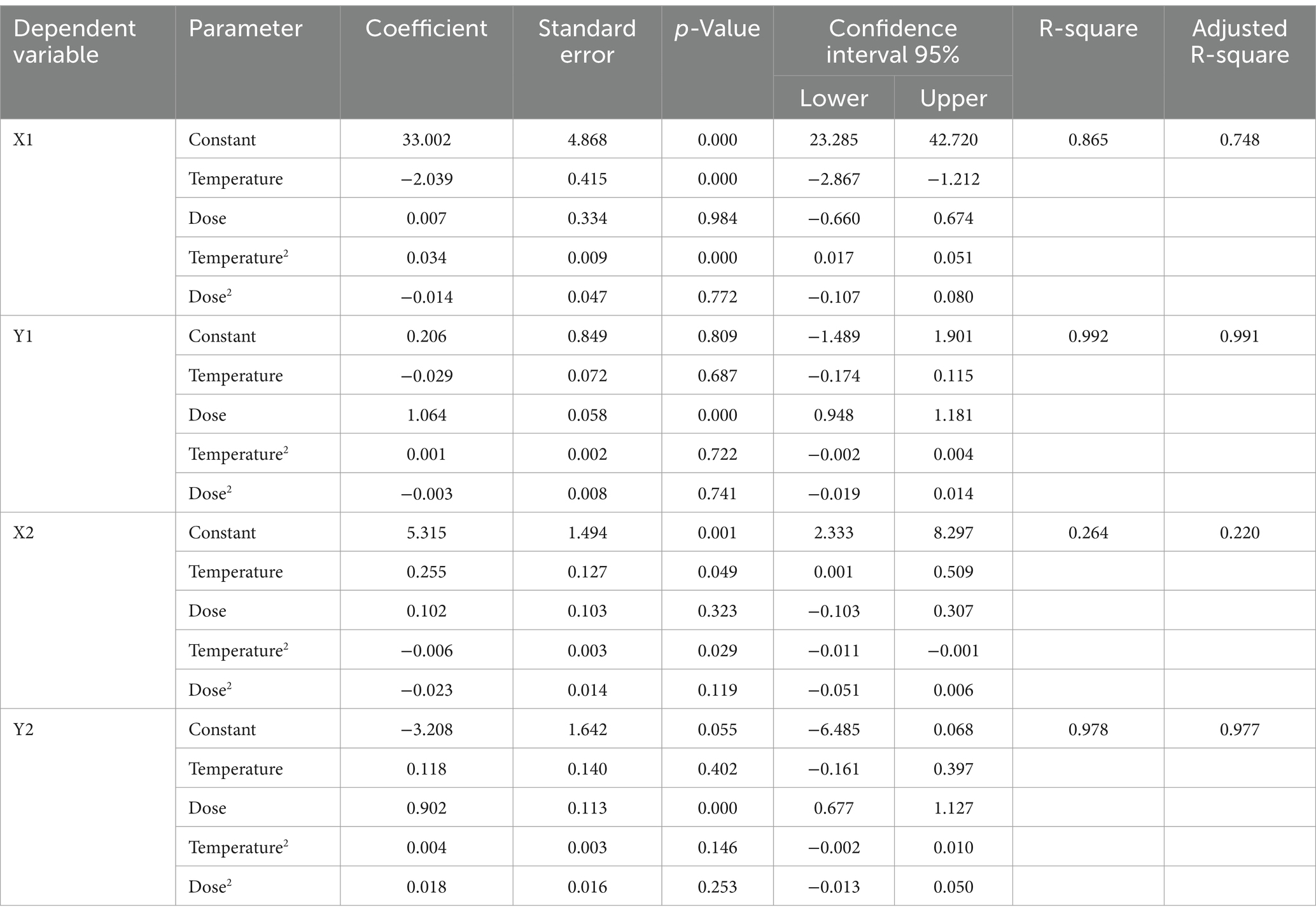
Table 2. Summary of the secondary modeling step for growth of Salmonella Infantis in chicken liver.

3.2.2 Secondary modeling of the dependent data for lag time or X1

Graphs of the PM_X1 data for lag time (Figure 6) and the SM_PR predictions of X1 as a function of dose and temperature indicated that observed and predicted values were in close agreement and that the moderate R² value for the SM_PR fit (Table 2) was from high variation of lag time among replicated storage trials as indicated by large standard deviations. The graphs in Figure 6 clearly show the nonlinear effect of temperature on lag time.

Figure 6

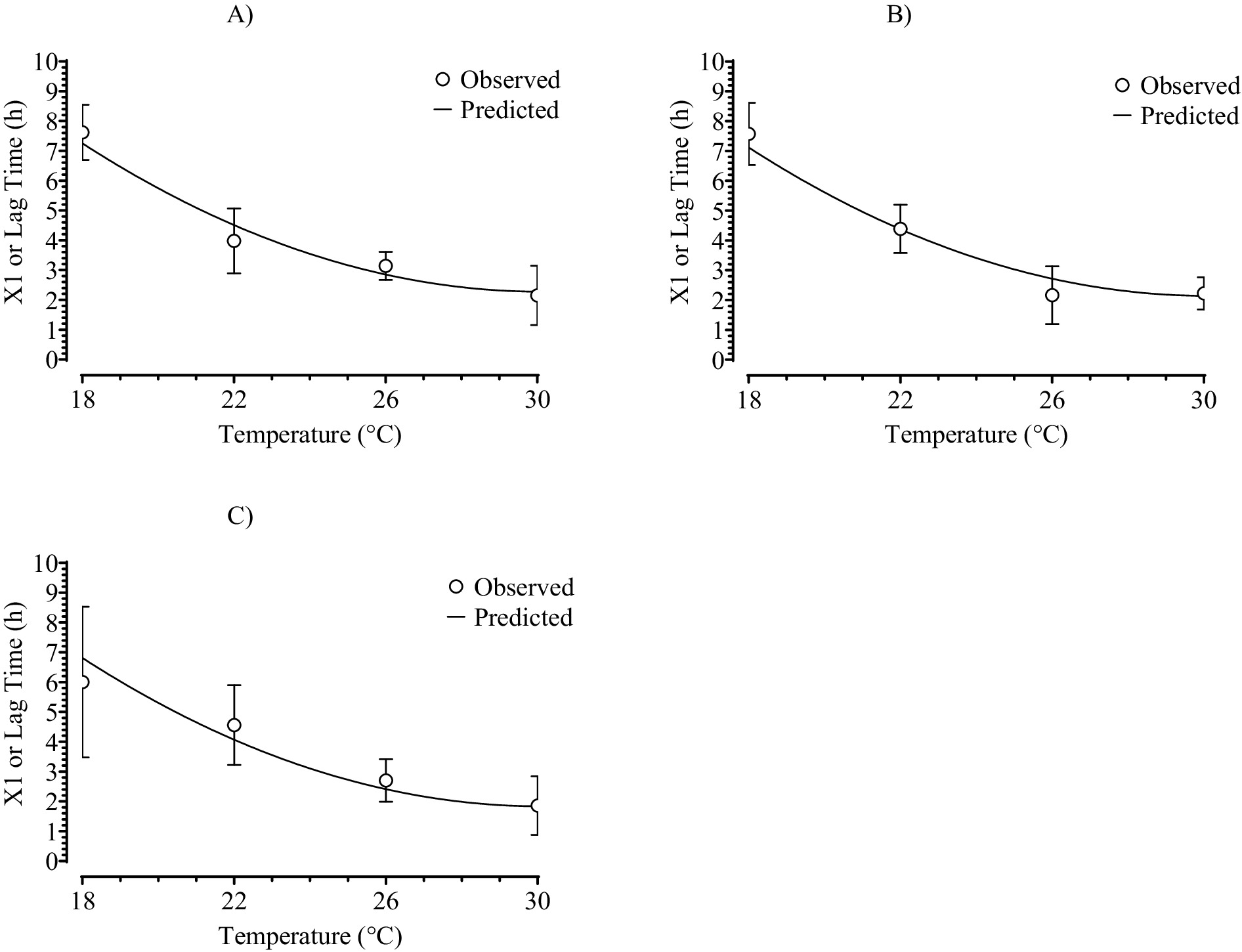
Figure 6. Fit of the polynomial regression, secondary model (SM_PR) to the dependent data for the three-phase linear, primary model parameter values for lag time or X1 as a function of doses of: (A) 10¹; (B) 10^3.5; or (C) 10⁶ and temperature (X-axis) for growth of Salmonella Infantis in chicken liver. Symbols are means ± standard deviation of results from six replicated storage trials and SM_PR fits.

3.2.3 Validation of the SM_PR predictions of the dependent data for lag time or X1

The APZ analysis (S10) indicated that the data used to develop the SM_PR for lag time satisfied the criteria for test data with answers of “yes” to Q1–Q3 in the decision tree for dependent data. In addition, the SM_PR for X1 displayed no local or global prediction problems as indicated by answers of “yes” to Q4–Q6 in the decision tree for dependent data (S10). In fact, the pAPZ for individual levels and combinations of independent variables and overall were ≥0.737 (analysis C in Table 1). These results were confirmed in Figure 7A where all relative residuals for X1 except three were in the partly or fully acceptable prediction zones. Therefore, the SM_PR for X1 was validated for the dependent data as indicated by an answer of “yes” to Q7 in the decision tree for dependent data (S10). Thus, SM_PR for X1 was eligible for validation for interpolation (Figure 2).

Figure 7

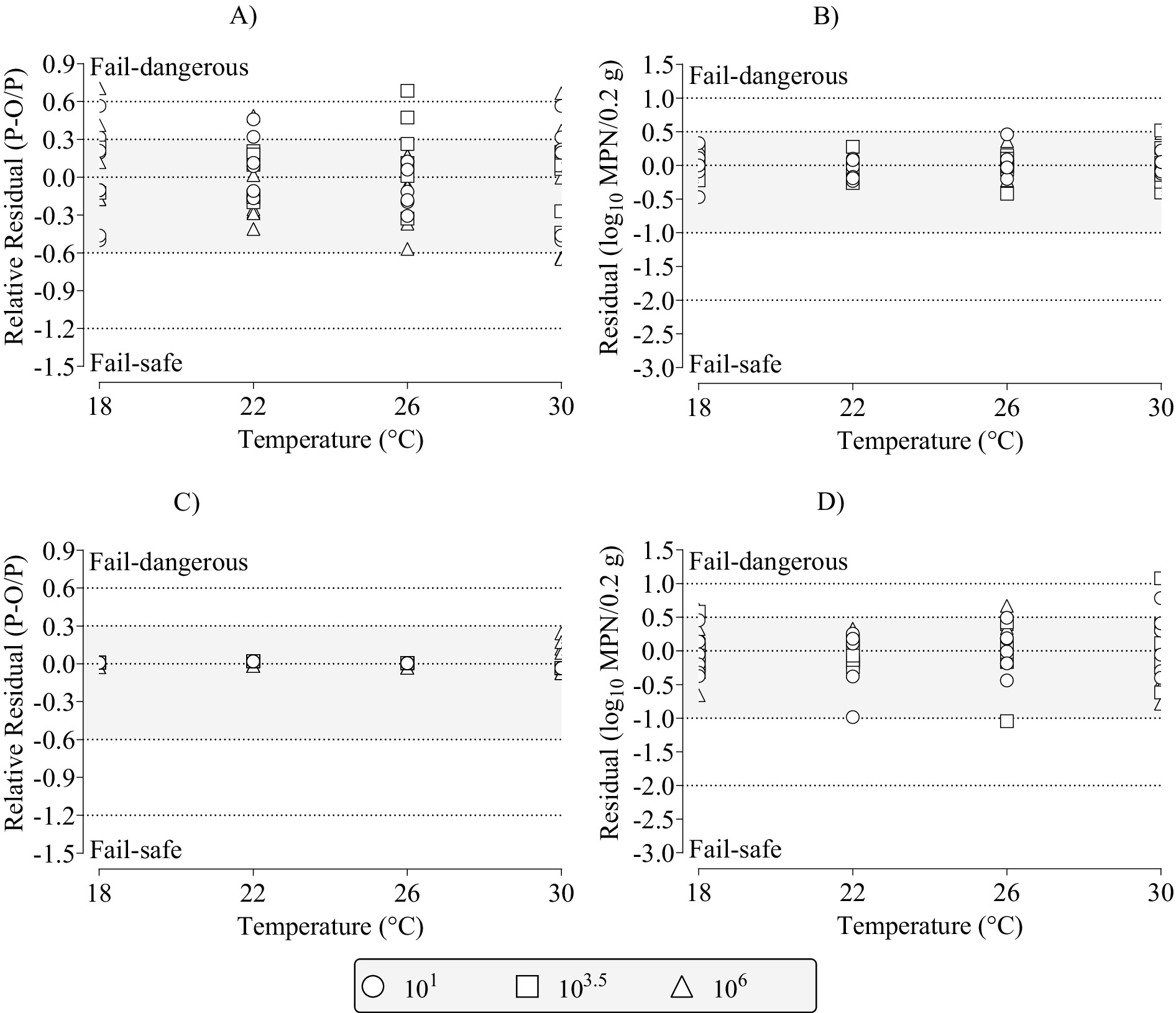
Figure 7. Distribution of relative residuals and residuals (observed–predicted) among the partly (dotted lines with no fill) and fully (dotted lines with gray fill) acceptable prediction zones for the polynomial regression, secondary model fits to the dependent data for the three-phase linear, primary model parameters of: (A) lag time (X1); (B) initial most probable number (Y1); (C) time to final most probable number (X2); and (D) final most probable number (Y2) for growth of Salmonella Infantis in chicken liver as a function of dose (10¹, 10^3.5, 10⁶), and temperatures of 18, 22, 26, or 30°C. P, predicted; O, observed; and MPN, most probable number.

3.2.4 Secondary modeling of the dependent data for initial most probable number or Y1

Graphs of the PM_3PL parameter data for initial MPN and the SM_PR predictions of Y1 as a function of the dose and temperature indicated that observed and predicted values were in close agreement (S12). In addition, there was a low variation of observed values of Y1 among replicated storage trials, which helped explain the high R² value for the SM_PR fit to these data (Table 2).

3.2.5 Validation of SM_PR predictions of the dependent data for initial most probable number or Y1

The APZ analysis (S13) indicated that the data used to develop the SM_PR for initial MPN satisfied the criteria for test data with answers of “yes” to Q1–Q3 in the decision tree for dependent data. In addition, the SM_PR for Y1 displayed no local or global prediction problems as indicated by answers of “yes” to Q4–Q6 in the decision tree for dependent data (S13). In fact, the pAPZ for individual levels and combinations of independent variables and overall were ≥0.995 (analysis E in Table 1). These results were confirmed in Figure 7B where all residuals for Y1 were in the partly and fully acceptable prediction zones. Therefore, the SM_PR for Y1 was validated for the dependent data as indicated by an answer of “yes” to Q7 in the decision tree (S13) and thus, was eligible for validation for interpolation (Figure 2).

3.2.6 Secondary modeling of the dependent data for time to final most probable number or X2

Graphs of the PM_3PL parameter data for time to final MPN and the SM_PR predictions of X2 as a function of the dose and temperature indicated that observed and predicted values were in close agreement (S12) even though the R² for the SM_PR was very low (Table 2). The time to final MPN was fixed at 8 h for all PM_3PL fits except four, which were for the combination of the highest dose (10⁶) and highest temperature (30°C) where three phases of growth were observed in four of six replicated storage trials. Thus, the standard deviation was zero for all combinations of dose and temperature, except the one mentioned. The graphs in S14 show the small but significant nonlinear effect of temperature on X2.

3.2.7 Validation of the SM_PR predictions of dependent data for X2

The APZ analysis indicated that the X2 data used to develop the SM_PR for time to final MPN satisfied the criteria for test data with answers of “yes” to Q1–Q3 in the decision tree for dependent data (S15). In addition, the SM_PR for X2 displayed no local or global prediction problems as indicated by answers of “yes” to Q4–Q6 in the decision tree for dependent data (S15). In fact, the pAPZ for individual levels and combinations of independent variables, and overall was = 1.00 (analysis G in Table 1). These results were confirmed in Figure 7C where all the relative residuals for X2 were in the partly or fully acceptable prediction zones. Therefore, the SM_PR for X2 was validated for dependent data as indicated by an answer of “yes” to Q7 in the decision tree (S15) and thus, was eligible for validation for interpolation (Figure 2).

3.2.8 Secondary modeling of the dependent data for Y2

Graphs of the PM_3PL parameter data for final MPN and the SM_PR predictions of Y2 as a function of the dose and temperature indicated that observed and predicted values were in close agreement (S16). In addition, there was a low variation of observed values among replicate storage trials, which explained the high R² value for the SM_PR fit to these data (Table 2).

3.2.9 Validation of SM_PR predictions of dependent data for Y2

The APZ analysis indicated that the PM_3PL data used to develop the SM_PR for final MPN satisfied the criteria for test data as indicated by answers of “yes” to Q1–Q3 in the decision tree for dependent data (S17). In addition, the SM_PR for Y2 displayed no local or global prediction problems as indicated by answers of “yes” to Q4–Q6 in the decision tree for dependent data (S17). In fact, the pAPZ for individual levels and combinations of independent variables and overall was ≥0.833 (analysis I in Table 1). These results were confirmed in Figure 7D where all residuals for Y2 except one were in the partly and fully acceptable prediction zones. Therefore, the SM_PR for Y2 was validated for the dependent data as indicated by an answer of “yes” to Q7 in the decision tree (S17) and thus, was eligible for validation for interpolation (Figure 2).

3.2.10 Validation of SM_PR predictions of independent data for interpolation of lag time or X1

Graphs of the independent data for interpolation of the PM_3PL parameter of lag time and SM_PR predictions of X1 as a function of dose and temperature (S18) indicated that observed and predicted values were not in as close agreement as they were for the dependent data (Figure 6). The APZ analysis (Figure 8) indicated that the independent data for X1 used to validate the SM_PR for interpolation satisfied the criteria for test data as indicated by answers of “yes” to Q2–Q5 in the decision tree. Thus, the test data were not used to develop the SM_PR; they were collected using the same methods as used to collect the dependent data; the values for the independent variables of dose, time, and temperature were intermediate to those of the dependent data; and there was a minimum of two prediction cases per combination of the independent variables.

Figure 8

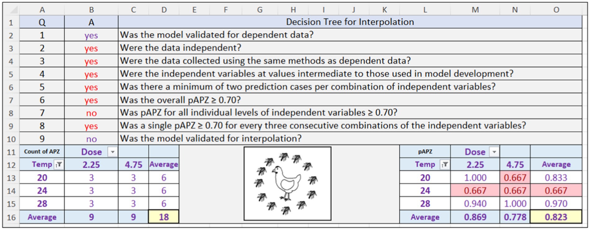
Figure 8. Screenshot of the Acceptable Prediction Zones (APZ) analysis in the Validation Software Tool for the polynomial regression, secondary model that predicts lag time (X1) of Salmonella Infantis in chicken liver as a function of dose (10^2.25, 10^4.75) and temperature (20, 24, 28°C). Results are for the independent data for interpolation. pAPZ, proportion of relative residuals in the partly and fully acceptable prediction zones.

Although the SM_PR for X1 had acceptable overall performance (pAPZ = 0.823) for the independent data for interpolation, it had a local prediction problem at 24°C (pAPZ = 0.667) resulting in an answer of “no” to Q7 in the decision tree (Figure 8 and analysis D in Table 1). These results were confirmed in S20A where three of the relative residuals for X1 were outside the partly and fully acceptable prediction zones. Therefore, the SM_PR for X1 failed validation for interpolation as indicated by an answer of “no” to Q9 in the decision tree for interpolation (Figure 8) and thus, was not eligible for validation for extrapolation (Figure 2). Rather, the course of action for this SM_PR may be to repair it by collecting more data. However, this is only necessary if it causes the TM_PR to fail validation, which was not the case.

3.2.11 Validation of SM_PR predictions of independent data for interpolation of initial MPN or Y1

Graphs of the independent data for interpolation of the PM_3PL parameter data for initial MPN and SM_PR predictions of Y1 as a function of dose and temperature (S21) indicated that observed and predicted values were in close agreement. This was confirmed by the APZ analysis (S22), which indicated that the independent data for Y1 used to validate the SM_PR for interpolation met the criteria for test data as indicated by answers of “yes” to Q2–Q5 in the decision tree. In addition, the SM_PR for Y1 had acceptable local and global performance with pAPZ ≥ 0.975 resulting in answers of “yes” to Q6–Q8 in the decision tree for interpolation (analysis F in Table 1). These results were confirmed in S20B where all residuals for Y1 were inside the partly and fully acceptable prediction zones. Therefore, the SM_PR for Y1 passed validation for interpolation as indicated by an answer of “yes” to Q9 in the decision tree (S22) and thus, was eligible for validation for extrapolation to another independent variable (Figure 2).

3.2.12 Validation of SM_PR predictions of the independent data for interpolation for time to final MPN or X2

Graphs of the independent data for interpolation of the PM_3PL parameter for time to final MPN and the SM_PR predictions of X2 as a function of dose and temperature are shown in S23. Because the last sampling time in these storage trials was 7 h, and the SM_PR was based on 8 h storage trials, a prediction bias of 12.7% occurred (analysis H in Table 1). Nonetheless, the APZ analysis (S24) indicated that the independent data for time to final MPN met the criteria for test data as indicated by answers of “yes” to Q2–Q5 in the decision tree. Also, the SM_PR for X2 did not have any local or global prediction problems as indicated by pAPZ of 1.00 (analysis H in Table 1) resulting in answers of “yes” to Q6–Q8 for model performance criteria in the decision tree for interpolation (S24). Thus, the observed prediction bias (S23), which was slightly fail-dangerous, was acceptable because all the relative residuals were in the fully acceptable prediction zone (S20C). Therefore, the SM_PR for X2 was validated for interpolation as indicated by an answer of “yes” to Q9 in the decision tree (S24) and thus, was eligible for validation for extrapolation to a new independent variable (Figure 2).

3.2.13 Validation of SM_PR predictions of the independent data for interpolation for final MPN or Y2

Graphs of the independent data for interpolation of the PM_3PL parameter data for final MPN and the SM_PR predictions of Y2 as a function of dose and temperature are shown in S25. Regardless of the storage temperature, the SM_PR made biased predictions of Y2 at a dose of 10^2.25 and unbiased predictions of Y2 at a dose of 10^4.75 (S25). Overall, the prediction bias was −0.524 log₁₀ MPN per 0.2 g of chicken liver (analysis J in Table 1). Nonetheless, the APZ analysis (S26) indicated that the independent data for Y2 used to validate the SM_PR for interpolation met the criteria for test data as indicated by answers of “yes” to Q2–Q5 in the decision tree. Also, the SM_PR for Y2 had no local or global performance problems with pAPZ ≥0.796 (analysis J in Table 1) resulting in answers of “yes” to Q6–Q8 in the decision tree for interpolation (S26). These results were confirmed in S20D where all the residuals for Y2 were in the partly and fully acceptable prediction zones. Therefore, the SM_PR for Y2 passed validation for interpolation as indicated by an answer of “yes” to Q9 in the decision tree for interpolation (S26) and thus, was eligible for validation for extrapolation to another independent variable (Figure 2).

3.2.14 Two-way analysis of variance

Figure 9 shows results of the two-way, ANOVA for the dependent data (panels A to C) and for the independent data for interpolation (panels D to F) for initial MPN or Y1 (panels A and D), lag time or X2 (panels B and E), and growth rate (panels C and F), which was calculated as {Y2-Y1}/{X2-X1}. Initial MPN was affected (p ≤ 0.05) by dose but not by temperature. Lag time and growth rate were affected (p ≤ 0.05) by temperature but not by dose. Thus, the growth of Salmonella Infantis in chicken liver was not affected by dose.

Figure 9

Figure 9. Two-way, analysis of variance results for the effects of dose, temperature, or their interaction on initial number or Y1 (A,D), lag time or X1 (B,E), and growth rate (C,F) for dependent data (A–C) or independent data for interpolation (D–F). Symbols are results for individual storage trials and lines are means.

3.3 Tertiary model construction and validation

3.3.1 Construction of the TM_PR for growth of Salmonella Infantis in chicken liver

The SM_PR for PM_3PL parameters X1, X2, Y1, and Y2 were incorporated into the PM_3PL to construct the TM_PR in an Excel spreadsheet (Figure 10). The TM_PR predicted the growth of Salmonella Infantis in chicken liver as a function of dose (10¹–10⁶), time (0–8 h) and temperature (18–30°C) for combinations of independent variables that were used and not used in TM_PR construction. In the example shown in Figure 10, the TM_PR predicted the growth of Salmonella Infantis in chicken liver for a temperature (25°C), times (0.1 h increments) and dose (10^1.5), not used in TM_PR construction. The TM_PR also predicted the PM_3PL parameters X1, Y1, X2, and Y2, which were used to calculate the growth rate of 0.484 {log₁₀ MPN/0.2 g} per h for the simulated combination of independent variables.

Figure 10

Figure 10. Three-phase linear, polynomial regression, tertiary model (TM_PR) and multiple layer feedforward neural network with two nodes in the hidden layer, tertiary model (TM_NN) for predicting growth of Salmonella Infantis in chicken liver as a function of dose (10¹–10⁶), time (0–8 h), and temperature (18–30°C). Temp, temperature; and Log and MPN, most probable number. The model was developed in Excel (Office 365, MicroSoft) and was simulated with NeuralTools (version 8.2, Lumivero).

3.3.2 Validation of the TM_PR for predicting the dependent MPN data

The ability of the TM_PR to predict dependent MPN data was assessed by graphing observed MPN values and predicted MPN values as a function of the independent variables (Figure 11). These graphs indicated good agreement between the observed and predicted MPN values. This was confirmed by conducting an APZ analysis (Figure 12). Here, the global pAPZ of the TM_PR for the dependent MPN data (n = 360) was 0.979 (analysis K in Table 1) and there were no local predictions problems with pAPZ ≥0.833 resulting in answers of “yes” to Q4 to Q6 in the decision tree for dependent MPN data (Figure 12). The acceptable performance of the TM_PR was further confirmed in the residual plots (S31) where all residuals except one were in the partly and fully acceptable prediction zones. In addition, the dependent MPN data satisfied the criteria for test data as indicated by answers of “yes” to Q1 to Q3 in the decision tree (Figure 12). Therefore, the TM_PR was validated for the dependent MPN data as indicated by an answer of “yes” to Q7 in the decision tree (Figure 12) and thus, was eligible for validation for interpolation (Figure 2).

Figure 11

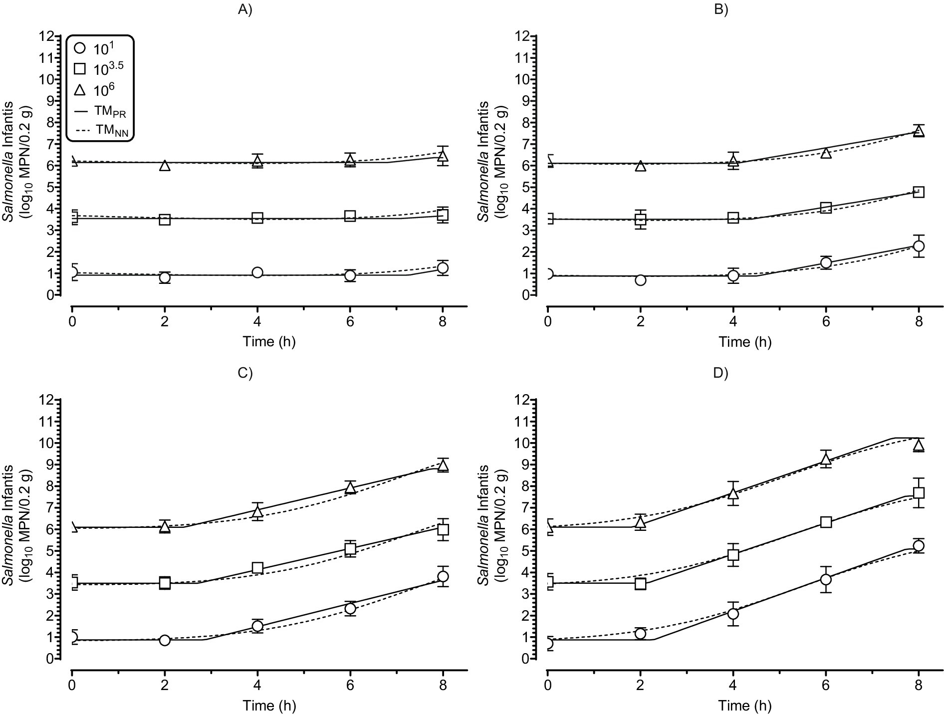
Figure 11. Tertiary model predictions of the dependent data for growth of Salmonella Infantis in chicken liver as a function of dose (10¹, 10^3.5, 10⁶), time (0–8 h), and temperatures of (A) 18°C; (B) 22°C; (C) 26°C; or (D) 30°C. Observed values (symbols) are means ± standard deviation of six replicated storage trials. MPN, most probable number; PR, polynomial regression; TM, tertiary model; and NN, multiple layer feedforward neural network with two nodes in the hidden layer.

Figure 12

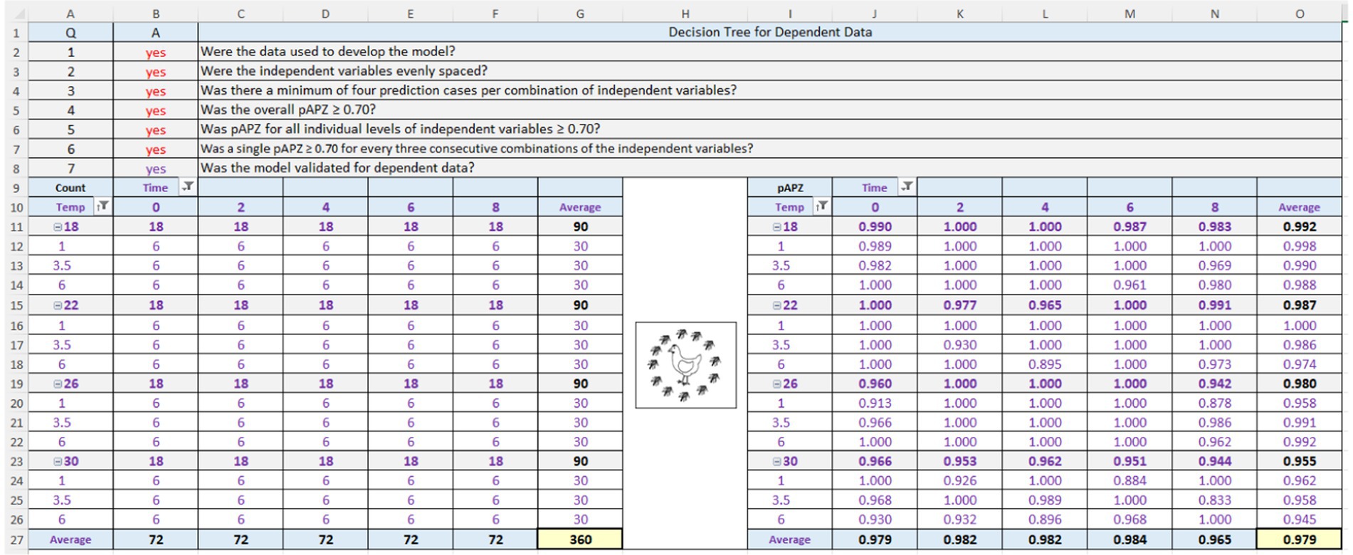
Figure 12. Screenshot of the Acceptable Prediction Zones (APZ) analysis in the Validation Software Tool for the three-phase linear, polynomial regression, tertiary model (TM_PR) that predicts the growth of Salmonella Infantis in chicken liver over time (0, 2, 4, 6, or 8 h) for individual combinations of dose (10¹, 10^3.5, or 10⁶) and temperature (18, 22, 26, or 30°C). Results are for the most probable number (MPN) data used in TM_PR construction or the dependent MPN data (n = 360).

3.3.3 Validation of the TM_PR for predicting the independent MPN data for interpolation

The ability of the TM_PR to predict the independent MPN data for interpolation was assessed by graphing the observed and predicted MPN values as a function of the independent variables (S32). These graphs indicated good but less agreement between observed and predicted MPN values than seen with the dependent MPN data (Figure 11). Nonetheless, the APZ analysis (S33) indicated that the TM_PR provided acceptable predictions of the independent data for interpolation with pAPZ ≥0.667 (analysis L in Table 1) resulting in answers of “yes” to Q6–Q8 in decision tree for interpolation (S33). In fact, the global pAPZ was 0.968, which was slightly lower than that for the dependent MPN data (analysis K in Table 1). The acceptable performance of the TM_PR for the independent MPN data for interpolation was confirmed in the residual plots (S34) where all residuals except one were in the partly and fully acceptable prediction zones. In addition, the independent MPN data for interpolation satisfied the criteria for test data as indicated by answers of “yes” to Q2–Q5 in the decision tree for interpolation (S33). Therefore, the TM_PR was validated for interpolation as indicated by an answer of “yes” to Q9 in the decision tree for interpolation (S33) and thus, was eligible for validation for extrapolation to another independent variable (Figure 2).

3.3.4 Construction of the TM_NN for predicting growth of Salmonella Infantis in chicken liver

A multiple-layer feedforward neural network with two nodes in the hidden layer, tertiary model (TM_NN) was developed in Excel (Office 365, MicroSoft) and was simulated with NeuralTools (version 8.2, Lumivero) (Figure 10). The TM_NN predicted the growth of Salmonella Infantis in chicken liver as a function of dose (10¹–10⁶), time (0–8 h), and temperature (18–30°C) for combinations of the independent variables that were used and not used in TM_NN construction. In the example shown in Figure 10, the TM_NN predicted the growth of Salmonella Infantis in chicken liver for a combination of temperature (25°C), dose (10^1.5), and times (0.1 h increments) not used in TM_NN construction. Unlike the TM_PR, the TM_NN does not predict lag time and growth rate, which is an important feature for some model users. Thus, to meet stakeholder needs, the final TM (Figure 10) included the TM_PR and TM_NN.

The simulations in Figures 10, 11 show that the TM_PR and TM_NN make similar predictions of the growth of Salmonella Infantis in chicken liver. This conclusion is supported by the APZ and two-way ANOVA analyses that are provided next.

3.3.5 Validation of the TM_NN for predicting the dependent MPN data

The ability of the TM_NN to predict dependent MPN data was assessed by graphing observed and predicted values as a function of the independent variables (Figure 11). These graphs indicated good agreement between observed and predicted MPN values and low variation of growth among replicated storage trials as indicated by small standard deviations of the MPN values. To confirm the visual appraisal of the performance of the TM_NN for the dependent data, an APZ analysis was performed (Figure 13). The global pAPZ of the TM_NN for the dependent data (n = 360) was 0.976 (analysis M in Table 1) and there were no local predictions problems with pAPZ ≥0.830 resulting in answers of “yes” to Q5 and Q6 in decision tree for dependent data (Figure 13). This was confirmed further in the residual plots (S38) where all residuals except one were in the partly and fully acceptable prediction zones. In addition, the dependent MPN data satisfied the criteria for test data as indicated by answers of “yes” to Q1–Q3 in the decision tree (Figure 13). Therefore, the TM_NN was validated for the dependent MPN data as indicated by an answer of “yes” to Q7 in the decision tree (Figure 13) and thus, was eligible for validation for interpolation (Figure 2).

Figure 13

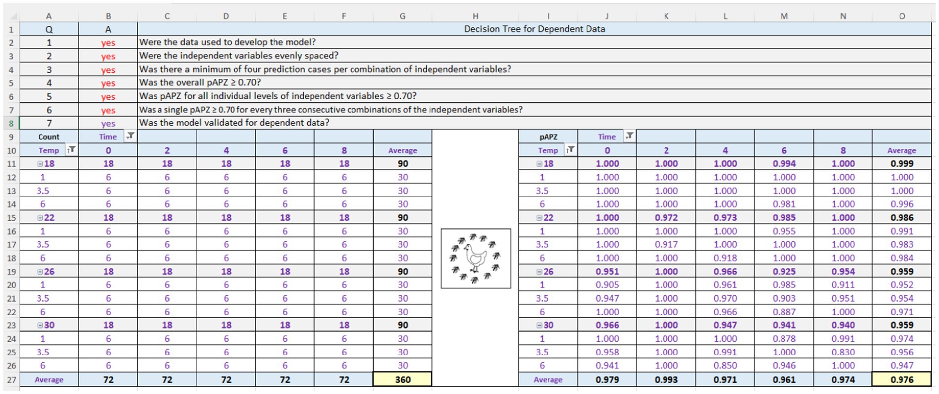
Figure 13. Screenshot of the Acceptable Prediction Zones (APZ) analysis in the Validation Software Tool (ValT) for the multiple layer feedforward neural network with two nodes in the hidden layer, tertiary model (TM_NN) that predicts the growth of Salmonella Infantis in chicken liver over time (0, 2, 4, 6, or 8 h) for individual combinations of dose (10¹, 10^3.5, or 10⁶) and temperature (18, 22, 26, or 30°C). Results are for the dependent data (n = 360).

3.3.6 Validation of the TM_NN for predicting independent MPN data for interpolation

The ability of the TM_NN to predict the independent MPN data for interpolation was assessed by graphing the observed and predicted values as a function of the independent variables (S32). These graphs indicated good but less agreement between observed and predicted MPN values than seen with the dependent MPN data (Figure 11). Nonetheless, the APZ analysis (S39) indicated that the TM_NN provided acceptable predictions of the independent MPN data for interpolation with pAPZ ≥0.709 (analysis N in Table 1) resulting in answers of “yes” to Q6–Q8 in the decision tree for interpolation (S39). Thus, there were no local or global prediction problems. In fact, the overall pAPZ was 0.968 (S39), which was slightly lower than that for the dependent MPN data (analysis M in Table 1).

The acceptable performance of the TM_NN for the independent MPN data for interpolation was confirmed in the residual plots (S40) where all residuals were in the partly and fully acceptable prediction zones. In addition, the independent MPN data for interpolation satisfied the criteria for test data as indicated by answers of “yes” to Q2–Q5 in the decision tree for interpolation (S39). Therefore, the TM_NN was validated for interpolation as indicated by an answer of “yes” to Q9 in the decision tree for interpolation (S39) and thus, was eligible for validation for extrapolation to another independent variable (Figure 2).

3.3.7 Comparison of the TM_PR and TM_NN for prediction bias and accuracy by two-way ANOVA

The mean residual, which was a measure of prediction bias, and the mean absolute residual, which was a measure of prediction accuracy, were compared as a function of the type of data (dependent or independent for interpolation), type of model (TM_PR or TM_NN), and their interaction (Figure 14). Prediction bias was not affected (p > 0.05) by type of data, type of model, or their interaction (Figure 14A). Likewise, prediction accuracy was not affected (p > 0.05) by type of data, type of model or their interaction (Figure 14B). These results indicated that, regardless of the type of data, the TM_PR and the TM_NN provided similar predictions of the growth of Salmonella Infantis in chicken liver as a function of dose (10¹–10⁶), time (0–8 h), and temperature (18–30°C). Thus, either TM can be used with confidence to predict the growth of Salmonella Infantis in chicken liver as a function of the investigated and modeled independent variables. The TM could be incorporated into a risk assessment model by using probability distributions for the independent variables and Monte Carlo simulation (Oscar, 2009, 2024b).

Figure 14

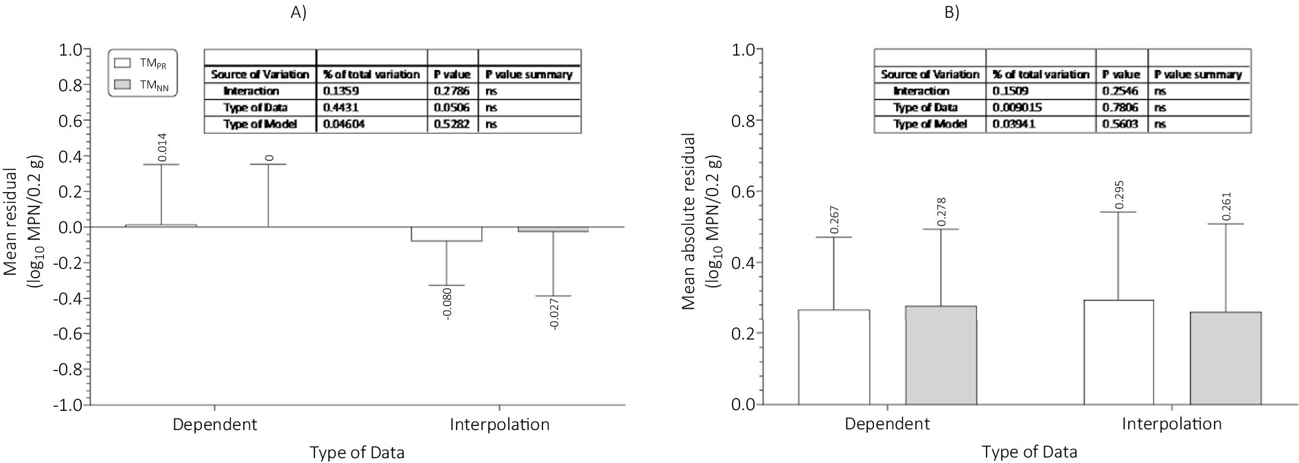
Figure 14. Comparison of (A) mean residual or prediction bias; and (B) mean absolute residual or prediction accuracy of the three-phase linear, polynomial regression, tertiary model (TM_PR) and the multiple layer feedforward neural network with two nodes in the hidden layer, tertiary model (TM_NN) for the dependent data used in model construction and the independent data for interpolation used in model validation for growth of Salmonella Infantis in chicken liver. There were no significant (ns; p > 0.05) differences between the TM_PR and TM_NN for prediction bias or accuracy.

4 Discussion

The primary processing of poultry consists of a series of unit operations like bleed-out, scalding, defeathering, evisceration, washing, chilling, and cold storage. Within a unit operation one or more Salmonella events like growth, death, survival, or cross-contamination may occur. Thus, to simulate changes in Salmonella on poultry during primary processing, TM for each unit operation and associated Salmonella event would need to be constructed, validated, and linked. The key to linking TM for Salmonella and poultry is considering the previous unit operation when collecting data for TM construction and validation.

In the current study, the unit operation targeted for construction and validation of TM for growth of Salmonella in chicken livers was secondary processing, which could occur in a processing plant or in a restaurant, institution, or home kitchen. The relevant previous unit operation was cold storage. Consequently, the chicken livers were inoculated at 4°C to simulate a previous history of refrigerated storage. In addition, the chicken liver samples (0.2 g) were inoculated with doses (10¹–10⁶) of a serotype (Infantis) of Salmonella found in the chicken livers after cold storage in a previous study (Oscar, 2021). After inoculation, the chicken liver samples were held at times (0–8 h) and temperatures (18–30°C) relevant to a secondary processing deviation of temperature abuse. Thus, the MPN data used to construct and validate the TM were collected under dynamic conditions of temperature as the chicken liver samples warmed from 4°C to the test temperature. In this way, growth under dynamic conditions of temperature for the simulated scenario was a built-in feature of the TM.

In the present study, the construction and validation of the TM_PR for growth of Salmonella Infantis in chicken liver was more time consuming and complex than the construction of the TM_NN because it involved three construction steps instead of one and 12 APZ analyses instead of two. Stated differently, construction and validation of the TM_NN was faster and simpler because it combined the primary, secondary, and tertiary steps of TM construction (Figure 1) into one step. Considering that the performance of the TM_PR and TM_NN for predicting the growth of Salmonella Infantis in chicken liver was the same, it was concluded that the one step, neural network method was the better one for TM construction and validation.

Although this was the first study, to the best of my knowledge, to compare performance of TM_PR and TM_NN, other studies have compared these two modeling methods at the PM and SM steps. For example, Schepers et al. (2000) compared a PM_NN with four weights to a set of PM_R with four parameters and found equal performance for fitting growth curves of Lactobacillus helviticus in broth culture. Jeyamkondan et al. (2001) compared SM_NN and SM_R for predicting generation time and lag time as a function of temperature for two pathogens and one spoilage organism. They found similar performance except for some test data sets for interpolation, where the SM_R performed better than the SM_NN. Thus, like the current results for TM, neural network (NN) and regression (R) methods result in similar performance of PM and SM in predictive microbiology. This conclusion is supported by other studies (Garcia-Gimeno et al., 2005; Hajmeer et al., 1997) with some comparing NN and R_logistic for no growth/growth models (Hajmeer and Basheer, 2003; Kuroda et al., 2019; Valero et al., 2007).

Validation of models is important because it provides users with confidence that model predictions are reliable (Zwietering et al., 1994). In addition, it helps modelers identify problems that can be repaired to provide users with better models (Oscar, 2005b). In the present study, models were validated using established criteria for test data, model performance, and model validation (Oscar, 2020b). The criteria for test data ensured that model validation process was complete, unbiased, and accurate. The criteria for model performance and validation ensured that an objective decision was made about model performance and validation.

In the present study, the validation process was more time consuming and complex for the TM_PR than the TM_NN because, in addition to the TM, it involved validation of the PM and 4 SM for dependent data and interpolation. Nonetheless, both TM had similar performance, and both were validated for interpolation. The only issue occurred in the SM for lag time, which had a local prediction problem for interpolation at 24°C. However, it was a prediction problem that did not result in a prediction problem in the TM_PR. Consequently, the SM for lag time was not repaired.

The method used to construct the TM_PR in the present study was to develop SM for all PM_3PL parameters (Y1, X1, X2, Y2) and then incorporate them back into the PM_3PL from which they were derived (Oscar, 2002). Once this was done, the TM_PR was validated for interpolation in two steps. First, by comparing predicted MPN values to observed MPN values used in TM_PR construction. Second, by comparing predicted MPN values to observed MPN values not used in TM_PR construction but collected at intermediate values of the independent variables using the same methods used to collect the MPN data used in TM_PR construction. However, this approach to TM construction and validation differs from other recent studies in which growth of Salmonella in food was investigated and modeled using regression-based methods.

In the study of Omac (2024), growth of Salmonella on carrots as a function of dose (10¹, 10²), time, and temperature (5–37°C) was investigated and modeled. The growth curves were fitted to the Baranyi PM, which had parameters for initial cell concentration, maximum cell concentration, maximum growth rate, and lag time. Regression-based SMs were developed for PM parameters. The SM were compared to the dependent data but not to independent data for interpolation. The SM were not incorporated back into the Baranyi PM to construct and validate a TM. The dependent data did not satisfy the test data criteria of the APZ method (Oscar, 2023).

In the study of Noviyanti et al. (2024), growth of Salmonella in chicken juice and meat as a function of time (0–39 h) and temperature (10–25°C) was investigated and modeled. The growth curves were fitted to the Baranyi PM with parameters of initial log count, maximum specific growth rate, lag time, time to reach stationary growth phase, final log count, and increase in log count from initial to final log count. A SM was developed for growth rate, whereas no SM were developed for the other PM parameters. Predictions of the SM for growth rate were compared to published data for growth rate obtained with other data collection and modeling methods. Thus, a TM was not constructed and validated.

In the study of Haque et al. (2024), growth of Salmonella in ground pork was investigated and modeled as a function of time, temperature (10–40°C), fat level (5, 25%), and microbial competition. The growth curves were fitted using a competition PM with parameters of initial density, maximum specific growth rate, and common saturation time. A SM for maximum specific growth as a function of temperature was developed, whereas SM for the other primary model parameters were not. A TM was constructed by inserting the SM for maximum specific growth rate into the differential form of the Baranyi PM with parameters of initial density, maximum specific growth rate, maximum population density, and physiological state. Maximum population density was calculated using the PM_3PL of Buchanan et al. (1997), whereas a fixed value for physiological state was determined by trial and error. Although TM predictions were compared to an independent set of data, they did not satisfy the test data criteria of the APZ method (Oscar, 2023). In addition, TM predictions were not compared to the dependent data.

In the study of Jia et al. (2020), growth of Salmonella in ground chicken as a function of time, temperature (8–33°C), and microbial competition was investigated and modeled. A one-step regression-based method was used to construct the TM. Thus, like the present study, SM for the PM parameters were used in the PM from which they were derived to construct the TM. Also, like the current study, the ability of the TM to predict the log count data used to construct the TM was evaluated. Although the ability of the TM to predict the log count data not used in TM construction was evaluated, the independent data did not satisfy the test data criteria for interpolation of the APZ method (Oscar, 2023) because they were not obtained at intermediate values of the independent variables. Nonetheless, the one step regression method used by Jia et al. (2020) is like the one step method used in the current study to construct a TM_NN in that it was a faster and simpler way to construct a TM.

5 Conclusion

In conclusion, the results of the current study indicated that it is less time consuming and complex to construct and validate a TM for growth of Salmonella Infantis in chicken liver without sacrificing TM performance using a one-step, NN method rather than a three-step, PR_3PL method. Both the TM_PR and TM_NN were validated for interpolation in this study using the test data, model performance, and model validation criteria of the APZ method in ValT (Oscar, 2020b). Thus, they can be used with confidence to predict the growth of Salmonella Infantis in chicken liver during a secondary processing deviation as a function of dose (10¹–10⁶), time (0–8 h), and temperature (18–30°C). A disadvantage of the TM_NN for some is that it does not predict the lag time and growth rate of Salmonella in chicken liver like the TM_PR. Thus, to meet stakeholder needs, the final TM deployed from the present study will include both the TM_PR and TM_NN. A common use of such TM is to determine if a process deviation results in significant growth of the pathogen, which is usually an increase of 1-log or more. If yes, the process is considered in need of correction, and the food is considered unsafe.

Data availability statement

The raw data supporting the conclusions of this article will be made available by the authors without undue reservation.

Author contributions

TO: Conceptualization, Data curation, Formal analysis, Funding acquisition, Investigation, Methodology, Project administration, Resources, Software, Supervision, Validation, Visualization, Writing – original draft, Writing – review & editing.

Funding

The author(s) declare that no financial support was received for the research and/or publication of this article.

Conflict of interest

The author declares that the research was conducted in the absence of any commercial or financial relationships that could be construed as a potential conflict of interest.

Generative AI statement

The author declares that no Gen AI was used in the creation of this manuscript.

Publisher’s note

All claims expressed in this article are solely those of the authors and do not necessarily represent those of their affiliated organizations, or those of the publisher, the editors and the reviewers. Any product that may be evaluated in this article, or claim that may be made by its manufacturer, is not guaranteed or endorsed by the publisher.

Supplementary material

The Supplementary material for this article can be found online at: https://www.frontiersin.org/articles/10.3389/fsufs.2025.1565247/full#supplementary-material

References

Bovill, R., Bew, J., Cook, N., D'Agostino, M., Wilkinson, N., and Baranyi, J. (2000). Predictions of growth for listeria monocytogenes and Salmonella during fluctuating temperature. Int. J. Food Microbiol. 59, 157–165. doi: 10.1016/s0168-1605(00)00292-0

Crossref Full Text | Google Scholar

Buchanan, R. L., Whiting, R. C., and Damert, W. C. (1997). When is simple good enough: a comparison of the Gompertz, Baranyi and three-phase linear models for fitting bacterial growth curves. Food Microbiol. 14, 313–326. doi: 10.1006/fmic.1997.0125

Crossref Full Text | Google Scholar

Garcia-Gimeno, R. M., Hervas-Martinez, C., Rodriguez-Perez, R., and Zurera-Cosano, G. (2005). Modelling the growth of Leuconostoc mesenteroides by artificial neural networks. Int. J. Food Microbiol. 105, 317–332. doi: 10.1016/j.ijfoodmicro.2005.04.013

Crossref Full Text | Google Scholar

Hajmeer, M., and Basheer, I. (2003). Comparison of logistic regression and neural network-based classifiers for bacterial growth. Food Microbiol. 20, 43–55. doi: 10.1016/S0740-0020(02)00104-1

Crossref Full Text | Google Scholar

Hajmeer, M. N., Basheer, I. A., and Najjar, Y. M. (1997). Computational neural networks for predictive microbiology II. Application to microbial growth. Int. J. Food Microbiol. 34, 51–66. doi: 10.1016/s0168-1605(96)01169-5

Crossref Full Text | Google Scholar

Hanson, H., Hancock, W. T., Harrison, C., Kornstein, L., Waechter, H., Reddy, V., et al. (2014). Creating student sleuths: how a team of graduate students helped solve an outbreak of Salmonella Heidelberg infections associated with kosher broiled chicken livers. J. Food Prot. 77, 1390–1393. doi: 10.4315/0362-028X.JFP-13-564

Crossref Full Text | Google Scholar

Haque, M., Wang, B., Mvuyekure, A. L., and Chaves, B. D. (2024). Modeling the growth of Salmonella in raw ground pork under dynamic conditions of temperature abuse. Int. J. Food Microbiol. 422:110808. doi: 10.1016/j.ijfoodmicro.2024.110808

Crossref Full Text | Google Scholar

Jeyamkondan, S., Jayas, D. S., and Holley, R. A. (2001). Microbial growth modelling with artificial neural networks. Int. J. Food Microbiol. 64, 343–354. doi: 10.1016/S0168-1605(00)00483-9

Crossref Full Text | Google Scholar

Jia, Z., Peng, Y., Yan, X., Zhang, Z., Fang, T., and Li, C. (2020). One-step kinetic analysis of competitive growth of Salmonella spp. and background flora in ground chicken. Food Control 117:107103. doi: 10.1016/j.foodcont.2020.107103

Crossref Full Text | Google Scholar

Jung, Y., Porto-Fett, A. C. S., Shoyer, B. A., Henry, E., Shane, L. E., Osoria, M., et al. (2019). Prevalence, levels, and viability of Salmonella in and on raw chicken livers. J. Food Prot. 82, 834–843. doi: 10.4315/0362-028X.JFP-18-430

Crossref Full Text | Google Scholar

Khan, S., McWhorter, A. R., Andrews, D. M., Underwood, G. J., Moore, R. J., Van, T. T. H., et al. (2024). Dust sprinkling as an effective method for infecting layer chickens with wild-type Salmonella typhimurium and changes in host gut microbiota. Environ. Microbiol. Rep. 16:e13265. doi: 10.1111/1758-2229.13265

Crossref Full Text | Google Scholar

Kuroda, S., Okuda, H., Ishida, W., and Koseki, S. (2019). Modeling growth limits of Bacillus spp. spores by using deep-learning algorithm. Food Microbiol. 78, 38–45. doi: 10.1016/j.fm.2018.09.013

Crossref Full Text | Google Scholar

Lanier, W. A., Hale, K. R., Geissler, A. L., and Dewey-Mattia, D. (2018). Chicken liver-associated outbreaks of campylobacteriosis and salmonellosis, United States, 2000-2016: identifying opportunities for prevention. Foodborne Pathog. Dis. 15, 726–733. doi: 10.1089/fpd.2018.2489

Crossref Full Text | Google Scholar

Noviyanti, F., Mochida, M., and Kawasaki, S. (2024). Predictive modeling of Salmonella spp. growth behavior in cooked and raw chicken samples: real-time PCR quantification approach and model assessment in different handling scenarios. J. Food Sci. 89, 2410–2422. doi: 10.1111/1750-3841.17020

Crossref Full Text | Google Scholar

Omac, B. (2024). Modeling the growth behavior of Salmonella spp. in grated carrots inoculated with different inoculum levels stored at various temperatures. J. Food Saf. 44:e13150. doi: 10.1111/jfs.13150

Crossref Full Text | Google Scholar

Oscar, T. P. (2002). Development and validation of a tertiary simulation model for predicting the potential growth of Salmonella typhimurium on cooked chicken. Int. J. Food Microbiol. 76, 177–190. doi: 10.1016/s0168-1605(02)00025-9

Crossref Full Text | Google Scholar

Oscar, T. P. (2005a). Development and validation of primary, secondary and tertiary models for predicting growth of Salmonella Typhimurium on sterile chicken. J. Food Prot. 68, 2606–2613. doi: 10.4315/0362-028x-68.12.2606

Crossref Full Text | Google Scholar

Oscar, T. P. (2005b). Validation of lag time and growth rate models for Salmonella Typhimurium: acceptable prediction zone method. J. Food Sci. 70, M129–M137. doi: 10.1111/j.1365-2621.2005.tb07103.x

Crossref Full Text | Google Scholar

Oscar, T. P. (2009). General regression neural network and Monte Carlo simulation model for survival and growth of Salmonella on raw chicken skin as a function of serotype, temperature, and time for use in risk assessment. J. Food Prot. 72, 2078–2087. doi: 10.4315/0362-028x-72.10.2078

Crossref Full Text | Google Scholar

Oscar, T. P. (2015). Neural network model for survival and growth of Salmonella enterica serotype 8,20:-:z₆ in ground chicken thigh meat during cold storage: extrapolation to other serotypes. J. Food Prot. 78, 1819–1827. doi: 10.4315/0362-028X.JFP-15-093

Crossref Full Text | Google Scholar

Oscar, T. P. (2018). Development and validation of a neural network model for predicting growth of Salmonella Newport on diced Roma tomatoes during simulated salad preparation and serving: extrapolation to other serotypes. Int. J. Food Sci. Technol. 53, 1789–1801. doi: 10.1111/ijfs.13767

Crossref Full Text | Google Scholar

Oscar, T. P. (2020a). Predictive model for growth of Salmonella Newport on Romaine lettuce. J. Food Saf. 40:e12786. doi: 10.1111/jfs.12786

Crossref Full Text | Google Scholar

Oscar, T. P. (2020b). Validation software tool (ValT) for predictive microbiology based on the acceptable prediction zones method. Int. J. Food Sci. Technol. 55, 2802–2812. doi: 10.1111/ijfs.14534

Crossref Full Text | Google Scholar

Oscar, T. P. (2021). Monte Carlo simulation model for predicting Salmonella contamination of chicken liver as a function of serving size for use in quantitative microbial risk assessment. J. Food Prot. 84, 1824–1835. doi: 10.4315/JFP-21-018

Crossref Full Text | Google Scholar

Oscar, T. P. (2023). “Acceptable prediction zones method for the validation of predictive models for foodborne pathogens” in Basic protocols in predictive food microbiology. ed. V. O. Alvarenga. 1st ed (New York, NY: Humana Press), 185–208.

Google Scholar

Oscar, T. P. (2024a). Development and validation of a predictive model for growth of Salmonella Infantis in ground Turkey. J. Food Prot. 87:100387. doi: 10.1016/j.jfp.2024.100387

Crossref Full Text | Google Scholar

Oscar, T. P. (2024b). Poultry food assess risk model for Salmonella and chicken gizzards: III. Dose consumed step. J. Food Prot. 87:100242. doi: 10.1016/j.jfp.2024.100242

Crossref Full Text | Google Scholar

Porto-Fett, A. C. S., Shoyer, B. A., Shane, L. E., Osoria, M., Henry, E., Jung, Y., et al. (2019). Thermal inactivation of Salmonella in pate made from chicken liver. J. Food Prot. 82, 980–987. doi: 10.4315/0362-028X.JFP-18-423

Crossref Full Text | Google Scholar

Procura, F., Bueno, D. J., Bruno, S. B., and Roge, A. D. (2019). Prevalence, antimicrobial resistance profile and comparison of methods for the isolation of Salmonella in chicken liver from Argentina. Food Res. Int. 119, 541–546. doi: 10.1016/j.foodres.2017.08.008

Crossref Full Text | Google Scholar

Rivera-Perez, W., Barquero-Calvo, E., and Zamora-Sanabria, R. (2014). Salmonella contamination risk points in broiler carcasses during slaughter line processing. J. Food Prot. 77, 2031–2034. doi: 10.4315/0362-028X.JFP-14-052

Crossref Full Text | Google Scholar

Schepers, A. W., Thibault, J., and Lacroix, C. (2000). Comparison of simple neural networks and nonlinear regression models for descriptive modeling of Lactobacillus helveticus growth in pH-controlled batch cultures. Enzyme Microbiol. Technol. 26, 431–445. doi: 10.1016/s0141-0229(99)00183-0

Crossref Full Text | Google Scholar

Thayer, D. W., Muller, W. S., Buchanan, R. L., and Phillips, J. G. (1987). Effect of NaCl, pH, temperature, and atmosphere on growth of Salmonella typhimurium in glucose-mineral salts medium. Appl. Environ. Microbiol. 53, 1311–1315. doi: 10.1128/aem.53.6.1311-1315.1987

Crossref Full Text | Google Scholar

Valero, A., Hervas, C., Garcia-Gimeno, R. M., and Zurera, G. (2007). Product unit neural network models for predicting the growth limits of Listeria monocytogenes. Food Microbiol. 24, 452–464. doi: 10.1016/j.fm.2006.10.002

Crossref Full Text | Google Scholar

Wang, J., Fenster, D. A., Vaddu, S., Bhumanapalli, S., Kataria, J., Sidhu, G., et al. (2024). Colonization, spread and persistence of Salmonella (typhimurium, Infantis and Reading) in internal organs of broilers. Poult. Sci. 103:103806. doi: 10.1016/j.psj.2024.103806

Crossref Full Text | Google Scholar

Whiting, R. C. (1995). Microbial modeling in foods. Crit. Rev. Food Sci. Nutr. 32, 467–494.

Google Scholar

Yokoyama, E., Ando, N., Ohta, T., Kanada, A., Shiwa, Y., Ishige, T., et al. (2015). A novel subpopulation of Salmonella enterica serovar Infantis strains isolated from broiler chicken organs other than the gastrointestinal tract. Vet. Microbiol. 175, 312–318. doi: 10.1016/j.vetmic.2014.11.024

Crossref Full Text | Google Scholar

Zwietering, M. H., Cuppers, H. G. A. M., deWit, J. C., and van 'T Riet, K. (1994). Evaluation of data transformations and validation of a model for the effect of temperature on bacterial growth. Appl. Environ. Microbiol. 60, 195–203. doi: 10.1128/aem.60.1.195-203.1994

Crossref Full Text | Google Scholar