A point source model to represent heat distribution without calculating the Joule heat during radiofrequency ablation

Introduction

Radio Frequency Ablation (RFA) has been used for the treatment of focal primary and secondary liver malignancies as a minimally invasive, image-guided alternative to standard surgical resection (Berjano, 2006; Blachier et al., 2013). Computational simulations have been used to simulate the electrical thermal processes during the RFA and to predict the outcome of ablation treatment (Payne et al., 2010; Schumann et al., 2010). At the frequencies employed in RF ablation (300kHz − 1 MHz) and within the area of interest (the electrical power is deposited within a small radius around the active electrode), the tissues can be considered as a purely resistive medium, as the displacement currents are negligible. Using a quasi-static approach, the distributed heat source q (Joule loss) is given by (Doss, 1982)

$q=\vec{J}.\vec{E}=\sigma |\nabla V{|}^2(1)$

where $\vec{J},\vec{E},\sigma$ and V denote respectively the current density, the electric field intensity, the electrical conductivity (S/m) and the voltage. In the literature, the voltage is assumed to be constant on the surface of the RF electrode probe needle and the potential field generated around the probe is solved numerically using the Laplace equation (Prakash, 2010)

$\sigma \mathrm{\Delta }V=0(2)$

Here σ is assumed to be spatially homogeneous (Panescu et al., 1995; Tungjiktkusolmun et al., 2002; Ahmed et al., 2008). This model has to be applied on a very thin probe tip. Therefore, for better accuracy in the numerical simulation, a finer mesh is required in turn increases the computational cost. Solving Equation 2 together with bioheat equation (Pennes, 1948), cell-death model (O’Neill et al., 2011) and appropriate initial and boundary conditions to provide infeasible prediction time. Moreover, the accurate position of the entire electrode probe is not always available in CT scan images. On contrary, the calculated Joule heat losses are very sensitive to the probe position (Khlebnikov and Muehl, 2010). Alternatively, if the analytical solution of the Joule heat model is known, then the computational cost could reduce. Since the analytical solution of the Joule heat model on the liver domain is not easy to obtain, independent of the whole electrode geometry in the tissue, estimating the Joule heat during the RF ablation is a better choice to reduce the computational cost.

In this study, an alternative model is proposed to represent the RFA heat deposition without the need for Joule heat computation because the tissue near the probe receives significant Joule heat whereas tissue far away from the probe receives a negligible amount of heat (Schramm et al., 2007; Haemmerich, 2010). The proposed Gaussian distributed point source model uses a few voxels containing the electrode probe to represent the RFA power deposition. This novel model is validated against conventional Joule heat computation. Further, this model is employed on retrospective clinical data for validation.

Bioheat equation and cell death model

The RFA treatment requires the treatment prediction to kill a minimal amount of cancer cells. The bioheat equation predicts the temperature distribution around the tumour cells. The governing bioheat equation (Pennes, 1948) is given by

$\rho C\frac{\partial T}{\partial t}=\nabla .k\nabla T-{\rho }_b{C}_b{\omega }_b\left(T-T_a\right)+Q_r(3)$

where ρ and ρ_b denote respectively density of the blood and tissue, C and C_b denote the heat capacity of tissue and blood respectively, k is thermal conductivity, ω_b is the blood perfusion, T_a is the arterial temperature and Q_r is the power source term generate by RF probe which can be calculated by the Joule heat model or estimated by the point source model as explained later. The boundary and initial conditions are given by.

$T=37°C\text{on\hspace{0.17em}Circular/spherical\hspace{0.17em}sides}(4)$

$\frac{\partial T}{\partial n}=0\text{on\hspace{0.17em}probes\hspace{0.17em}surface}(5)$

$T\left(0\right)=37°C(6)$

Upon solving the above equations, the temperature distribution around the cells is known. Based on the temperature distribution the cell death model (O’Neill et al., 2011) predicts the alive and dead cells.

$\frac{dA}{dt}=-k_{f}A+k_b\left(1-A-D\right)(7)$

$\frac{dD}{dt}=k_f\left(1-A-D\right)(8)$

$k_f=k_{f_0}{e}^{\frac{T}{T_k}}\left(1-A\right)(9)$

Here A is the fraction of alive cells, D is the fraction of the dead cells, k_f and k_b denote the forward and backward constants to describe the rate of change from alive cells to dead cells and vice versa. $k_{f_0}$ is the scaling factor and T_k denotes the rate of the exponential increase with temperature.

Apart from obtaining the source term from either the Joule heat model or the point source model, the bioheat model is solved numerically using the finite element method on a finer mesh domain, whereas the cell-death model is solved using traditional finite difference method.

To provide justification for the point source model in place of the Joule heat model for the source term, needle geometry has to be explained. The next section explains the needle geometry and then followed by that the Joule heat model is explained.

Needle geometry

The multi-array needle (Figure 1) comes with a different number of needles AngioDynamics (2022b,a) ranging from 3 to 9. In this study, we used nine arrays plus an active trocar tip AngioDynamics (2022a). During the treatment, the needle is inserted inside the organ for heating which used to be either the centre of the tumour or a point near the tumour. This point is known as the target point or the intersection point. For each needle in the array, the target point, another endpoint and the midpoint between these two are used as point sources for our model.

FIGURE 1

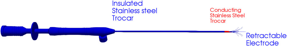
FIGURE 1. RFA needle geometry: RITA Starburst XL needle.

Joule heat model

In order to validate our point source model, it is necessary to compare the electric potential, the heat source term and the temperature obtained from both the Joule heat model and the point source model. We have tested our model in both two-dimension and three-dimensional models. In order to generate a proper point source model, let us first simulate the Joule heat model. The Joule heat model is simulated on unit circular and unit sphere geometry respectively on 2D and 3D. The needle is placed at the centre of the geometry. For the two-dimensional model, we have generated a finite element mesh on a circular disc where three array needle is placed at the centre of the disc as shown in Figure 2. For a three-dimensional model, finite element mesh on a sphere geometry with nine arrays needle at the centre of the sphere is generated as shown in Figure 3.

FIGURE 2

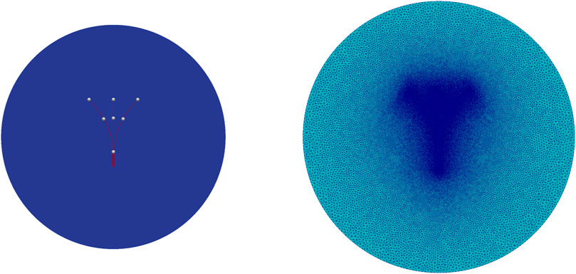
FIGURE 2. Two-dimensional needle geometry for case (2) (left) and adaptive finite element mesh used in the simulation. Mesh generated using Gmsh (Geuzaine and Remacle, 2020) (right).

FIGURE 3

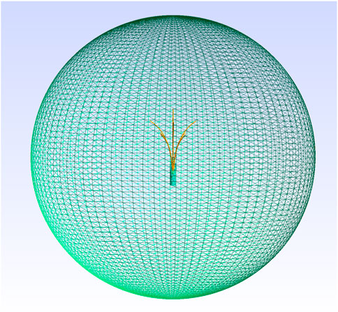
FIGURE 3. 3D Geometry and adaptive finite element mesh used in the simulation. Mesh generated using Gmsh (Geuzaine and Remacle, 2020).

The governing equations of the Joule heat model is given by

$\sigma \mathrm{\Delta }V=0(10)$

The boundary conditions for the electric potential are the following.

$V=a^{+}\text{on\hspace{0.17em}tips\hspace{0.17em}surface}(11)$

$V=a^{-}\text{on\hspace{0.17em}circular\hspace{0.17em}sides}(12)$

$\frac{\partial V}{\partial n}=0\text{on\hspace{0.17em}shaft\hspace{0.17em}surface}(13)$

Upon solving these equations for V, we can obtain the source term for the bioheat model as follows:

$Q_r=\sigma |\nabla V{|}^2(14)$

where σ is the electrical conductivity.

Analytical derivation

Geometry, electrical and thermal properties play an important role in the power deposition distribution of the treatment. Different manufacturers produce different kinds of probes for radiofrequency ablation. The study presented here is based on the RITA Starburst XL multi-array needle (Figure 1) and RITA 1500X RITA generator. However, the analytical results obtained here can also be applied to other types of ablation probes with proper changes.

Method of moments

The analysis starts by solving the charge distribution on a line conductor of finite length, a simplified geometry of the electric probe. Coulomb repulsion pushes the charge out towards the ends, just as the charge on a solid conductor flows to the surface. However, an explicit analytical solution to the charge distribution is an ill-posed problem in the scientific community (Griffiths and Li, 1996).

In the present study, our probe needle is modelled as a thin, conducting wire of length L and radius r oriented along the x axis as shown in Figure 4. Since the radius of the wire is very small, the electric (Coulomb) potential of the wire can be expressed using the following integral

${\varphi }_e\left(\vec{\mathbf{x}}\right)=\underset{0}{\overset{L}{\int }}\frac{q_e\left(x^{\prime }\right)d{x}^{\prime }}{4\pi \epsilon |\vec{\mathbf{x}}-\overrightarrow{{\mathbf{x}}^{\prime }}|}(15)$

where q_e is the charge density and ɛ is the electric constant. The conducting wire is subdivided into N segments ${\{I_j=[x_{j-1},x_j]\}}_{j=1}^N$ each of length Δx and the charge density of each subsegment is assumed to have a value q_j (j = 1, 2, …, N). Therefore, Equation 15 becomes

${\varphi }_e\left(\vec{\mathbf{x}}\right)=\frac{2\pi r}{4\pi \epsilon }\sum _{j=1}^N{q}_j\underset{I_j}{\int }\frac{d{x}^{\prime }}{|\vec{\mathbf{x}}-\overrightarrow{{\mathbf{x}}^{\prime }}|}(16)$

FIGURE 4

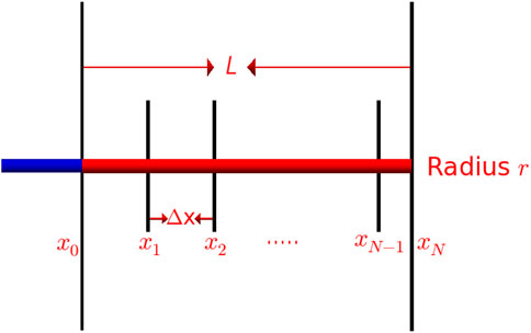
FIGURE 4. Thin conducting wire.

Let us fix the source points on the wire axis and the observation point on the wire’s surface (Gibson, 2008) which ensures that there is no singularity in the integrand. The denominator of the integrand becomes

$|\vec{x}-\overrightarrow{x^{\prime }}|=\sqrt{{\left(x-x^{\prime }\right)}^2+r^2}(17)$

Let us assume uniform charge density except for the endpoints (Andrews, 1997). Therefore, we assign the charge density as

$q_j=\left\{\begin{array}{cc}{q}_a\hfill & j=\mathrm{2,3},..,N-1\hfill \\ q_b\hfill & j=1,N\hfill \end{array}\right.$

Substituting q_j values and Equation 17 into Equation 16, we obtain

${\varphi }_e\left(\vec{x}\right)=\frac{1}{2\epsilon }\left(q_a\underset{\mathrm{\Delta }x}{\overset{\left(N-1\right)\mathrm{\Delta }x}{\int }}\frac{1}{\sqrt{{\left(x-x^{\prime }\right)}^2+r^2}}d{x}^{\prime }+q_b\underset{I_1\cup I_N}{\int }\frac{1}{\sqrt{{\left(x-x^{\prime }\right)}^2+r^2}}d{x}^{\prime }\right)(18)$

It is easy to verify that

$\int \frac{1}{\sqrt{{\left(x-x^{\prime }\right)}^2+r^2}}d{x}^{\prime }=\log \left(\sqrt{r^2+{\left(x-x^{\prime }\right)}^2}+x^{\prime }-x\right)(19)$

Under the following assumptions: $4\ll N\ll \frac{L}{r}$ and $\frac{r}{\mathrm{\Delta }x}\ll 1$, we evaluate the values of ϕ_e at x = x₀ = 0 and $x=x_{\frac{N}{2}}=\frac{L}{2}$

${\varphi }_e\left(0\right)\approx \frac{r}{2\epsilon }\left[q_b\log \frac{2L}{Nr}+q_a\log N+\frac{q_b}{N}\right](20)$

${\varphi }_e\left(\frac{L}{2}\right)\approx \frac{r}{2\epsilon }\left[\frac{2q_b}{N}+2q_a\log \frac{L}{r}+\frac{2q_b}{N}\right](21)$

Let γ_q denote the ratio of charge density at the ends of the conductor (q_b) to that at the remainder of the conductor (q_a). Since the electric potential on the conductor is constant, using ϕ_e(x) = V, 0 ≤ x ≤ L on (20) and 21, we obtain

${\gamma }_q=\frac{q_b}{q_a}=\frac{2\log \frac{L}{r}-\log N}{\log \frac{2L}{r}-\log N-\frac{3}{N}}(22)$

Let γ_P denote the ratio of power deposition at the ends of the conductor (P_b) to that at the remainder of the conductor (P_a). Since the power deposition(P) is proportional to square of the electric field and electric field (E) is proportional to the charge density(q), using P ∝ E² and E ∝ q in (22) yields

${\gamma }_P=\frac{P_b}{P_a}={\left(\frac{2\log \frac{L}{r}-\log N}{\log \frac{2L}{r}-\log N-\frac{3}{N}}\right)}^2(23)$

The RITA Starburst needle has 14 gauges ($\approx 1.6$mm) outer diameter and length 10 cm. However, the manufacturer AngioDynamics (2022b) supplies various types of needles whose length varies from 10 to 25 cm. In this study, we considered L = 10 cm and r = 0.8 mm. As per our assumption, N must satisfy $4\ll N\ll \frac{L}{r}=125$. The power ratio γ_P increases when the number of points N increases as given in Figure 5. As the variation in the charge near the end of the needle is represented more accurately as the number of segments increases. Therefore, the power deposition of the probe can be represented by N point sources along the needle, whilst two point sources located at the two ends of the needle deliver much higher power than other N − 2 point sources. The power ratio delivered by the needle ends and the needle middle cannot be obtained directly from γ(P) by assuming N = 3 as N = 3 does not satisfy the inequality $4\ll N\ll \frac{L}{r}=125$.

FIGURE 5

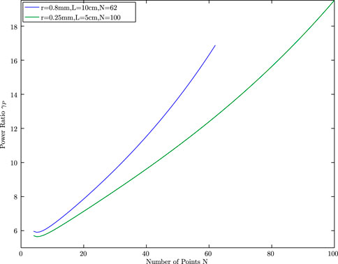
FIGURE 5. Ratio of power deposition ${\gamma }_P=\frac{P_b}{P_a}$.

Therefore, when the number of points known (k) is limited, k < N, then the power ratio can be modelled as:

${\eta }_P\left(k\right)=\frac{P_{\mathit{end}}}{P_{\mathit{mid}}}=\frac{P_b+\left(\frac{N}{k}-1\right)P_a}{\frac{N}{k}{P}_a}(24)$

Note that, when k = N, η_P = γ_P.

In the two-dimensional study, we considered three needles and divided them into the following three cases: 1) the number of point sources is four, three at the end of the tips and one at the intersection of three needles, 2) the number of point sources is seven, three located at the ends of the tips and 3 located at the middle of the tips and one at the intersection of three needles, k = 3, 3) the number of point sources is 13, three located at the end of the tips and the remaining 6 are located equally placed between the end tips and the intersection tips, k = 5. Figure 2 shows the two-dimensional geometry and the needle tips for case (2), k = 3.

For case (2), k = 3 and the power ratio from the endpoint to the midpoint is given by

${\eta }_P={\eta }_P\left(3\right)=\frac{P_{\mathit{end}}}{P_{\mathit{mid}}}=\frac{P_b+\left(\frac{N}{3}-1\right)P_a}{\frac{N}{3}{P}_a}(25)$

Figure 6 plots the ratio η_P against the range of N. The value η_P decays as N increases and finally converges to approximately 1.76, which is the power ratio we propose in our point source model. Note that, the power ratio changes when the length and diameter of the needle change. For instance, when r = 0.25 mm and L = 5cm, the power ratio η_P = 1.5 as given in Figure 6. Similarly when k changes, the power ratio changes as given in Figure 7.

FIGURE 6

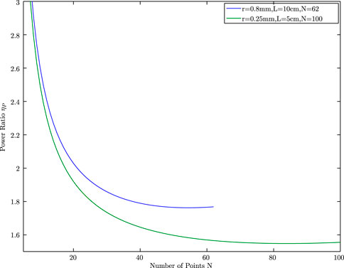
FIGURE 6. Power ratio ${\eta }_P=\frac{P_{\mathit{end}}}{P_{\mathit{mid}}}$.

FIGURE 7

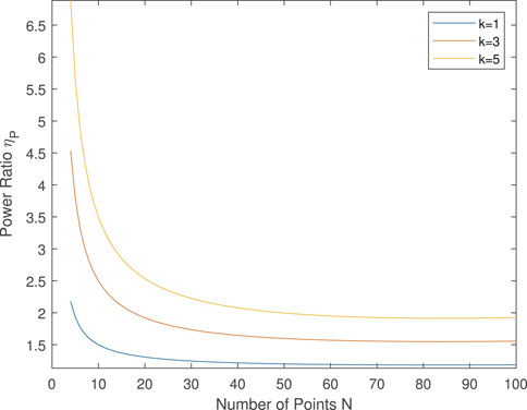
FIGURE 7. Power ratio ${\eta }_P=\frac{P_{\mathit{end}}}{P_{\mathit{mid}}}$ for different k and r = 0.25mm, L = 5 cm.

Point source model

The Laplace equation is invariant under rotation (Evans, 2010) and hence the radial solution is found and later the following fundamental solution of the Laplace equation is derived

$\varphi \left(x\right)=\left\{\begin{array}{cc}-\frac{1}{2\pi }\log |x|\hfill & n=2\hfill \\ \frac{1}{n\left(n-2\right)\alpha \left(n\right)}\frac{1}{|x{|}^{n-2}}\hfill & n\ge 3\hfill \end{array}\right.(26)$

defined for $x\in {\mathbb{R}}^n,x\ne 0$, where α(n) denotes the volume of the unit ball in ${\mathbb{R}}^n$. However, the Laplace equation is sometimes written as

$-\mathrm{\Delta }V={\delta }_0\text{in}{\mathbb{R}}^n(27)$

where δ₀ denotes the Dirac measure on ${\mathbb{R}}^n$. That is, the δ₀ provides a unit mass to the point 0. In the point source model development, unit mass or desired mass is given to the tip of the needle. To solve the above equation mollifier is defined as follows (Evans, 2010):

$\eta \left(x\right)=\left\{\begin{array}{cc}C{e}^{\frac{1}{|x{|}^2-1}}\hfill & if|x|<1\hfill \\ 0\hfill & if|x|\ge 1\hfill \end{array}\right.(28)$

where C is a constant selected so that ${\int }_{{\mathbb{R}}^n}\eta (x)dx=1$.

Based on the above discussion, the point source model is developed which is given by the Gaussian distribution

$Q_r\left(x\right)=\sum _{x_i\in \mathrm{\Omega }}\frac{1}{K}\sum _i{c}_i{e}^{-\frac{|x-x_i{|}^2}{2{\sigma }^2}}(29)$

where K and c_i are obtained by using needle parameters. Here Ω denotes the geometry domain, in our case circular domain or spherical domain. In real patient cases, it is a topological liver domain. Due to the analytical derivation, we have classified the c_i into two categories middle tips (green) and end tips (red) as shown in Figure 8.

FIGURE 8

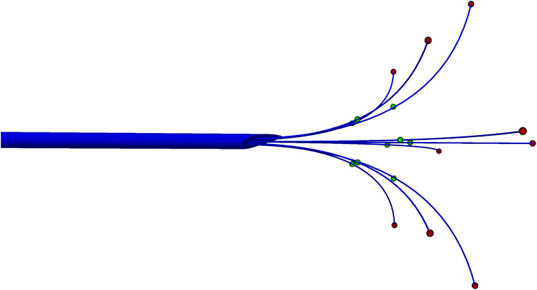
FIGURE 8. Points selected at the middle and end of each needle-array.

For the two-dimensional geometry, the point source model is given by.

$P\left(x,y\right)=\frac{1}{9}\frac{1}{{\left({\sigma }_P\sqrt{2\pi }\right)}^3}\sum _{\mathit{tip}}{c}_{\mathit{tip}}{e}^{-\frac{{\left(x-x_{\mathit{tip}}\right)}^2+{\left(y-y_{\mathit{tip}}\right)}^2}{2{\sigma }_P^2}}(30)$

$Q_r\left(x,y\right)=\sum _{\left(x,y\right)\in \mathrm{\Omega }}P\left(x,y\right)(31)$

Where the values of c_tip is obtained from γ_P. Further, the values of x_tip and y_tip are obtained using spline methods as follows: The parametric curve of the needle is given by

$\gamma \left(t\right)=a_2{t}^2+a_{1}t+a_0(32)$

Where

$t=\left\{\begin{array}{cc}-\frac{|a_1|+\sqrt{|a_1{|}^2+4|a_2|s}}{2|a_2|}\hfill & \text{if\hspace{0.17em}}|a_2|\ne 0\hfill \\ -\frac{s}{|a_1|}\hfill & \text{if\hspace{0.17em}}|a_2|=0\hfill \end{array}\right.$

For the three-dimensional geometry, the point source model is given by.

$P\left(x,y,z\right)=\frac{1}{24}\frac{1}{{\left({\sigma }_P\sqrt{2\pi }\right)}^3}\sum _{\mathit{tip}}{c}_{\mathit{tip}}{e}^{-\frac{{\left(x-x_{\mathit{tip}}\right)}^2+{\left(y-y_{\mathit{tip}}\right)}^2+{\left(z-z_{\mathit{tip}}\right)}^2}{2{\sigma }_P^2}}(33)$

$Q_r\left(x,y,z\right)=\sum _{\left(x,y,z\right)\in \mathrm{\Omega }}P\left(x,y,z\right)(34)$

In both cases, σ_P denotes the standard deviation for normal distribution with σ_P = 0.003 and

$c_{\mathit{tip}}=\left\{\begin{array}{cc}1.5\ast \text{power}\hfill & \text{for\hspace{0.17em}end\hspace{0.17em}tips}\hfill \\ 1.0\ast \text{power}\hfill & \text{for\hspace{0.17em}middle\hspace{0.17em}tips}\hfill \end{array}\right.(35)$

Here, k = 3 is considered. For k = 5, the c_tip values differ.

Numerical evaluation of the point source model and Joule heat model on a 2D simplified model

The Joule heat model is solved using the FEniCS(Dolfin 2019.2.0) (Alnæs et al., 2009), a finite element software tool, to obtain the electric potential and the source term Q_r for a two-dimensional circle geometry with a radius of 3 cm. Here the centre of the circle is located at the needle-trocar intersection point. The circle is discretized using Gmsh (Geuzaine and Remacle, 2020). The discretized mesh contains 117650 triangular elements with 58965 nodes.

In order to achieve a direct comparison between these two different approaches, the total power of the point source model and the Joule heat model is set to be 150W in both cases. This is equivalent to set parameter a^± = ±22.75V in the boundary conditions for the electric potential for the Joule heat model. For the point source model, the input power is considered as 150W. For k = 3, the input power values at the middle tips are 16.6W and the power values at the end tips are 25W. The values of all other parameters used in the bioheat equations are given in Table 1.

TABLE 1

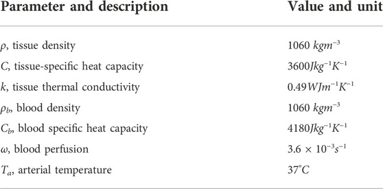
TABLE 1. Model parameters.

Figure 9 shows the ParaView visualization of the electric potential and heat source distribution, where more heat is distributed near the tip of the needle and it decreases as the distance from the tip increases.

FIGURE 9

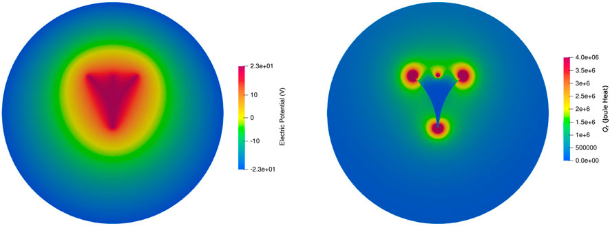
FIGURE 9. Electric potential (left) and the heat source term Q_r (right) from the Joule heat model.

For the Point source model, using simple python code for the same mesh, the values are computed and plotted using ParaView. Since the point source model follows the Gaussian distribution, the nature of the distribution is evident from Figure 10.

FIGURE 10

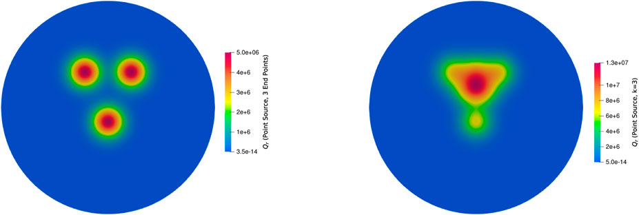
FIGURE 10. The heat source term Q_r from the point source model with 3 end points (left) and k = 3 (right).

The Q_r value computation using the Joule heat model and the point source model is respectively 7.13 and 4.5s for each iteration. When the power value changes depending on the temperature, computation of Q_r at each step is necessary. Therefore, for a 600s simulation with a 0.1s time step, it will take 11.8 h for the Joule heat model whereas 7.5 h for the point source model for Q_r computation. Apart from Q_r computation, we have to solve the bioheat equation and cell-death model at each time step. Since the matrix assembly and discretization are similar to the Joule heat model, for each time step, it takes 7.13s for the bioheat equation and 5.34s for the cell-death model. When the values of all parameters are constant, then FEniCS takes less time to compute the entire simulation. It takes approximately 1.5 h for the 600s ablation protocol which is due to the linear solvers. However, the power input is not constant in the practical application, therefore, the time required for the simulation while using the Joule heat model is approximately 13.3 h, whereas the point source model takes 9 h. With the help of graphics processing unit (GPU) parallelization (Mariappan et al., 2017; Voglreiter et al., 2018), it can be computed in minutes.

The heat distribution obtained by solving bioheat equation with Q_r term from Joule heat model and point source model is given Figure 11. Since the point source model is an approximation model to the Joule heat model, approximately 3°C degree difference is obtained which is negligible when the mesh is finer. Further, good accordance has been found in the temperature distribution and lesion between models. The predicted lesion zone of the point source model (293.7 mm²) is 95% of the Joule heating model (308.51 mm²) for 100s simulation when k = 3. When k = 5, the predicted lesion zone volume decreases to 217.69 mm², which is 70% of the Joule heat model volume, therefore, it is concluded that k = 3 provides the optimal lesion size. Figures 12, 13 provides the visual comparison between both dead cells.

FIGURE 11

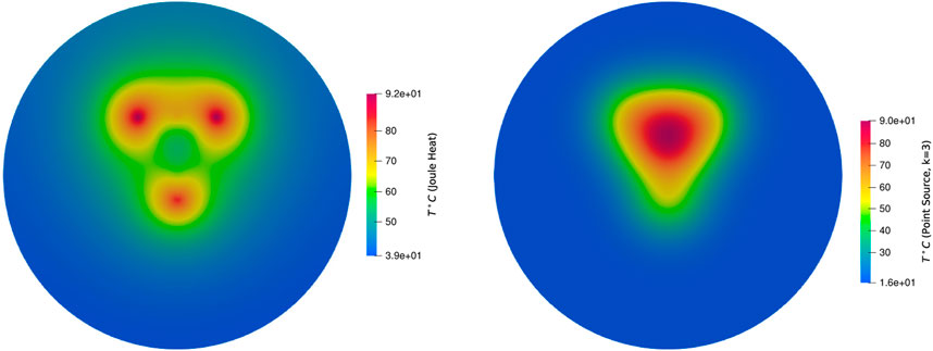
FIGURE 11. Temperature distribution by using bioheat equation with the source term from the Joule heat (left) and the point source model with k = 3 (right) for 100s.

FIGURE 12

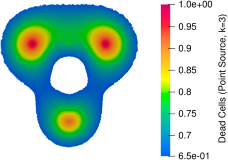
FIGURE 12. Dead cells obtained from temperature distribution where bioheat equation implemented with the source term from the Joule heat.

FIGURE 13

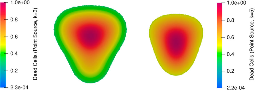
FIGURE 13. Dead cells obtained from temperature distribution where bioheat equation implemented with the source term from the point source model with k = 3 (middle) and with k = 5 (right) for 100s.

Numerical evaluation of the point source model and Joule heat model on a 3D model

The point source model has shown significantly good agreement with the Joule heat model. The point source model is already implemented in our GPU accelerated software tool to predict the lesion in real-time. Initially, the results were compared for pig models on a retrospective dataset. For example, Figure 14 shows the comparison between the dead cells obtained from the Joule heat (8891.1 mm³) model and the point source model (7912.4 mm³), which has 91% accuracy. The model parameters are the same as the two-dimensional geometry, whereas the finite element mesh has 1486412 triangular and tetrahedral elements with 237725 points. Since the solvers are already GPU accelerated, solvers with the point source model took 600s to produce the dead cells and solvers with the Joule heat model took 1000s to produce the dead cells.

FIGURE 14

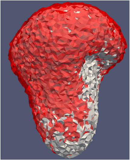
FIGURE 14. Dead cells by using Joule heat model (grey) and the point source model (red) for heat source term in the bioheat equation.

The point source model was already implemented in our ClinicIMPPACT project to simulate the temperature change during RFA and to predict the lesion zone (Mariappan et al., 2017; Voglreiter et al., 2018). Further, the real lesion and simulated lesions had good agreement while using the point source model during this project. The same model was used for clinical trials and found a good match. A good quantitative agreement has been reached between the model simulation and experimental measurements, which suggests that the point source model can be used as a substitute for the Joule heat computation in ablation treatment planning.

Limitations

This study has a few limitations on the model assumptions. Pennes bioheat equation has a few limitations (Nakayama and Kuwahara, 2008; Andreozzi et al., 2020) such as constant and uniform temperature instead of three temperature equations for three media (liver, vessels and tumour), other models are also used by researchers. This study uses only the Pennes bioheat equation. Since the aim of this study is to replace the Joule heat model with the point source model, the same point source model can be used in other modifications of the Pennes bioheat equation. Also, the haemodynamics fluid-structure interaction problems and the tissue contact force (Ana et al., 2018; Yan et al., 2020; Fang et al., 2022) on thermal lesion size are not taken into account in this study. These two studies could mainly impact the temperature distribution near larger vessels due to deformation. Further, the model parameters as given in Table 1 are treated as constant in this study. A few model parameters such as tissue-specific thermal conductivity (Trujillo and Berjano, 2013; Wu et al., 2016), the heat capacity of the tissue Yang et al. (2007, 2006), and blood perfusion (Schutt and Haemmerich, 2008; Singh and Melnik, 2019), can be included as temperature-dependent parameters.

$k\left(T\right)=\widetilde{k_0}+\mathrm{\Delta }k\left(T-T_0\right)(36)$

$C=C_t-\frac{\alpha }{\rho }\frac{dW\left(T\right)}{dT}(37)$

$W\left(T\right)=\left\{\begin{array}{c}0.778-0.778\times \text{exp}\left(\frac{T-106}{3.42}\right)\text{for}T\le 103°C\hfill \\ 0.0289T^3-0.8924T^2+919.6T-31573\hfill \\ \text{for}103°C<T\le 104°c\hfill \\ 0.778\times \text{exp}\left(\frac{T-80}{34.37}\right)\text{for}T\ge 104°C\hfill \end{array}\right.(38)$

${\omega }_b\left(T\right)=\left\{\begin{array}{c}\omega \text{for}T<60°C\hfill \\ 0\text{for}T\ge 60°C\hfill \end{array}\right.(39)$

Where $\widetilde{k_0}$ is the baseline thermal conductivity (W/m°C), Δk is the change in k due to temperature, T₀ is the reference temperature (°C) at which k₀ has been measured and α is the water latent heat content. With respect to the power ratio, one can also use dimensionless number such as Pomerantsev number (Kuneš, 2012) to scale the heat sources.

Conclusion

In this study, we have proposed a new point source model to approximate the power delivered from the needle without the need for a full solution of the electric field obtained using the Joule heat model. Both two-dimensional and three-dimensional simulation shows that the point source power model and the Joule heat model have good accordance with the minimum deviation between them. Also, the point source model reduces the computation time significantly as one of the finite element solvers is completely replaced by the point source model.

Data availability statement

The datasets presented in this article are not readily available because The two-dimensional datasets can be given, but the patient and pig datasets cannot be provided. Requests to access the datasets should be directed to panch.m@iittp.ac.in.

Author contributions

GB has contributed to the FEniCS code development for the comparison of two-dimensional models. PM has developed the simulation part of the three-dimensional model and implemented the same using C++ and CUDA programming. He contributed to the GPU acceleration and also wrote this manuscript. RF, one of the principal investigators of the ClinicIMPPACT project, helped to develop and validate the idea of point source model and three dimensional data set collections.

Funding

The data set collections and the RFA Guardian tool development was funded by the European Union’s Seventh Framework Programme for research, technological development and demonstration under grant agreement no 61088.

Acknowledgments

We thank Tingyin Peng, Claire Bost, David O’Neill, Stephen Payne, Phil Weir, Philip Voglreiter, Tuomas Alhonnoro, Mika Pollari, Michael Moche, Harald Busse, Jurgen Futterer, Horst Rupert Portugaller and Marina Kolesnik for their contribution in the project ClinicIMPPACT and detailed discussion for this model development.

Conflict of interest

Authors PM and RF were employed by the company NUMA Engineering Services Ltd.

The remaining author declare that the research was conducted in the absence of any commercial or financial relationships that could be construed as a potential conflict of interest.

Publisher’s note

All claims expressed in this article are solely those of the authors and do not necessarily represent those of their affiliated organizations, or those of the publisher, the editors and the reviewers. Any product that may be evaluated in this article, or claim that may be made by its manufacturer, is not guaranteed or endorsed by the publisher.

Supplementary material

The Supplementary Material for this article can be found online at: https://www.frontiersin.org/articles/10.3389/fther.2022.982768/full#supplementary-material

References

Ahmed, M., Liu, Z., Humphries, S., and Goldberg, S. N. (2008). Computer modeling of the combined effects of perfusion, electrical conductivity, and thermal conductivity on tissue heating patterns in radiofrequency tumor ablation. Int. J. Hyperth. 24, 577–588. doi:10.1080/02656730802192661

PubMed Abstract | CrossRef Full Text | Google Scholar

Alnæs, M. S., Logg, A., Mardal, K.-A., Skavhaug, O., and Langtangen, H. P. (2009). Unified framework for finite element assembly. Int. J. Comput. Sci. Eng. 4, 231–244. doi:10.1504/ijcse.2009.029160

CrossRef Full Text | Google Scholar

Ana, G. S., Juan, J. P., and Enrique, B. (2018). Should fluid dynamics be included in computer models for rf cardiac ablation by irrigated-tip electrodes. Biomed. Eng. OnLine 17, 43. doi:10.1186/s12938-018-0475-7

PubMed Abstract | CrossRef Full Text | Google Scholar

Andreozzi, A., Iasiello, M., and Tucci, C. (2020). An overview of mathematical models and modulated-heating protocols for thermal ablation. Adv. Heat Transf. 52, 489–541. doi:10.1016/bs.aiht.2020.07.003

CrossRef Full Text | Google Scholar

Andrews, M. (1997). Equilibrium charge density on a conducting needle. Am. J. Phys. 64, 846–850. doi:10.1119/1.18671

CrossRef Full Text | Google Scholar

Berjano, E. J. (2006). Theoretical modeling for radiofrequency ablation: State-of-the-art and challenges for the future. Biomed. Eng. OnLine 5, 24. doi:10.1186/1475-925X-5-24

PubMed Abstract | CrossRef Full Text | Google Scholar

Blachier, M., Leleu, H., Peck-Radosavljevic, M., Valla, D.-C., and Roudot-Thoraval, F. (2013). The burden of liver disease in europe: A review of available epidemiological data. J. Hepatology 58, 593–608. doi:10.1016/j.jhep.2012.12.005

PubMed Abstract | CrossRef Full Text | Google Scholar

[Dataset] AngioDynamics (2022a). Starburst model 1500x RF generator. New York: AngioDynamics.

Google Scholar

[Dataset] AngioDynamics (2022b). Starburst XL RFA generator. New York: AngioDynamics.

Google Scholar

Doss, J. D. (1982). Calculation of electric fields in conductive media. Med. Phys. 9, 566–573. doi:10.1118/1.595107

PubMed Abstract | CrossRef Full Text | Google Scholar

Evans, L. C. (2010). Partial differential equations. United States: American Mathematical Society.

Google Scholar

Fang, Z., Hongjun, W., Hanwei, Z., Michael, A. J. M., Wenjun, Z., Zhiqin, Q., et al. (2022). Radiofrequency ablation for liver tumors abutting complex blood vessel structures: Treatment protocol optimization using response surface method and computer modeling. Int. J. Hyperth. 39, 733–742. doi:10.1080/02656736.2022.2075567

PubMed Abstract | CrossRef Full Text | Google Scholar

Geuzaine, C., and Remacle, J.-F. (2020). Gmsh.

Google Scholar

Gibson, W. C. (2008). The method of moments in electromagnetics. Florida: Chapman & Hall/CRC.

Google Scholar

Griffiths, D. J., and Li, Y. (1996). Charge density on a conducting needle. Am. J. Phys. 64, 706–714. doi:10.1119/1.18236

CrossRef Full Text | Google Scholar

Haemmerich, D. (2010). Biophysics of radiofrequency ablation. Crit. Rev. Biomed. Eng. 38, 53–63. doi:10.1615/critrevbiomedeng.v38.i1.50

PubMed Abstract | CrossRef Full Text | Google Scholar

Khlebnikov, R., and Muehl, J. (2010). “Effects of needle placement inaccuracies in hepatic radiofrequency tumor ablation,” in 32nd Annual International Conference of the IEEE EMBS (Buenos Aires, Argentina: IEEE), 716–721.

PubMed Abstract | CrossRef Full Text | Google Scholar

Kuneš, J. (2012). 5 - thermomechanics, 173–283. doi:10.1016/B978-0-12-416013-2.00005-1

CrossRef Full Text | Google Scholar

Mariappan, P., Weir, P., Flanagan, R., Voglreiter, P., Alhonnoro, T., Pollari, M., et al. (2017). Gpu-based RFA simulation for minimally invasive cancer treatment of liver tumours. Int. J. Comput. Assist. Radiol. Surg. 12, 59–68. doi:10.1007/s11548-016-1469-1

PubMed Abstract | CrossRef Full Text | Google Scholar

Nakayama, A., and Kuwahara, F. (2008). A general bioheat transfer model based on the theory of porous media. Int. J. Heat Mass Transf. 51, 3190–3199. doi:10.1016/j.ijheatmasstransfer.2007.05.030

CrossRef Full Text | Google Scholar

O’Neill, D. P., Peng, T., Stiegler, P., Mayrhauser, U., Koestenbauer, S., Tscheliessnigg, K., et al. (2011). A three-state mathematical model of hyperthermic cell death. Ann. Biomed. Eng. 39, 570–579. doi:10.1007/s10439-010-0177-1

PubMed Abstract | CrossRef Full Text | Google Scholar

Panescu, D., Whayne, J. G., Fleischman, S. D., Mirotznik, M. S., Swanson, D. K., and Webster, J. G. (1995). Three-dimensional finite element analysis of current density and temperature distributions during radio-frequency ablation. IEEE Trans. Biomed. Eng. 42, 879–890. doi:10.1109/10.412649

PubMed Abstract | CrossRef Full Text | Google Scholar

Payne, S. J., Peng, T., O’Neill, D. P., Weihusen, A., Zidowitz, S., Moltz, J. H., et al. (2010). State of the art in computer-assisted planning, intervention, and assessment of liver-tumor ablation. Crit. Rev. Biomed. Eng. 38, 31–52. doi:10.1615/critrevbiomedeng.v38.i1.40

PubMed Abstract | CrossRef Full Text | Google Scholar

Pennes, H. H. (1948). Analysis of tissue and arterial blood temperatures in the resting human forearm. J. Appl. Physiology 1, 93–122. doi:10.1152/jappl.1948.1.2.93

CrossRef Full Text | Google Scholar

Prakash, P. (2010). Theoretical modeling for hepatic microwave ablation∼!2009-10-21∼!2009-12-30∼!2010-02-04∼!. Open Biomed. Eng. J. 4, 27–38. doi:10.2174/1874120701004020027

PubMed Abstract | CrossRef Full Text | Google Scholar

Schramm, W., Yang, D., Wood, B., Rattay, F., and Haemmerich, D. (2007). Contribution of direct heating, thermal conduction and perfusion during radiofrequency and microwave ablation. Open Biomed. Eng. J. 1, 47–52. doi:10.2174/1874120700701010047

PubMed Abstract | CrossRef Full Text | Google Scholar

Schumann, C., Rieder, C., Bieberstein, J., Weihusen, A., Zidowitz, S., Moltz, J. H., et al. (2010). Theoretical modeling for radiofrequency ablation: State-of-the-art and challenges for the future. Crit. Rev. Biomed. Eng. 38, 31–52. doi:10.1615/critrevbiomedeng.v38.i1.40

PubMed Abstract | CrossRef Full Text | Google Scholar

Schutt, D. J., and Haemmerich, D. (2008). Effects of variation in perfusion rates and of perfusion models in computational models of radio frequency tumor ablation. Med. Phys. 35, 3462–3470. doi:10.1118/1.2948388

PubMed Abstract | CrossRef Full Text | Google Scholar

Singh, S., and Melnik, R. (2019). “Radiofrequency ablation for treating chronic pain of bones: Effects of nerve locations,” in International Work-Conference on Bioinformatics and Biomedical Engineering (United States: Springer), 418–429.

CrossRef Full Text | Google Scholar

Trujillo, M., and Berjano, E. (2013). Review of the mathematical functions used to model the temperature dependence of electrical and thermal conductivities of biological tissue in radiofrequency ablation. Int. J. Hyperth. 29, 590–597. doi:10.3109/02656736.2013.807438

PubMed Abstract | CrossRef Full Text | Google Scholar

Tungjiktkusolmun, S., Staelin, S., Haemmerich, D., Tsai, J. Z., Cao, H., Webster, J. G., et al. (2002). Three-dimensional finite-element analyses for radio-frequency hepatic tumor ablation. IEEE Trans. Biomed. Eng. 49, 3–9. doi:10.1109/10.972834

PubMed Abstract | CrossRef Full Text | Google Scholar

Voglreiter, P., Mariappan, P., Pollari, M., Flanagan, R., Sequeiros, R. B., Portugaller, R. H., et al. (2018). RFA Guardian: Comprehensive simulation of radiofrequency ablation treatment of liver tumors. Sci. Rep. 8, 787. doi:10.1038/s41598-017-18899-2

PubMed Abstract | CrossRef Full Text | Google Scholar

Wu, X., Liu, B., and Xu, B. (2016). Theoretical evaluation of high frequency microwave ablation applied in cancer therapy. Appl. Therm. Eng. 107, 501–507. doi:10.1016/j.applthermaleng.2016.07.010

CrossRef Full Text | Google Scholar

Yan, S., Gu, K., Wu, X., and Wang, W. (2020). Computer simulation study on the effect of electrode–tissue contact force on thermal lesion size in cardiac radiofrequency ablation. Int. J. Hyperth. 37, 37–48. doi:10.1080/02656736.2019.1708482

PubMed Abstract | CrossRef Full Text | Google Scholar

Yang, D., Converse, M. C., Mahvi, D. M., and Webster, J. G. (2007). Expanding the bioheat equation to include tissue internal water evaporation during heating. IEEE Trans. Biomed. Eng. 54, 1382–1388. doi:10.1109/tbme.2007.890740

PubMed Abstract | CrossRef Full Text | Google Scholar

Yang, D., Converse, M. C., Mahvi, D. M., and Webster, J. G. (2006). Measurement and analysis of tissue temperature during microwave liver ablation. IEEE Trans. Biomed. Eng. 54, 150–155. doi:10.1109/tbme.2006.884647

PubMed Abstract | CrossRef Full Text | Google Scholar