Parameterizing Deep Water Percolation Improves Subsurface Temperature Simulations by a Multilayer Firn Model

Deep preferential percolation of melt water in snow and firn brings water lower along the vertical profile than a laterally homogeneous wetting front. This widely recognized process is an important source of uncertainty in simulations of subsurface temperature, density, and water content in seasonal snow and in firn packs on glaciers and ice sheets. However, observation and quantification of preferential flow is challenging and therefore it is not accounted for by most of the contemporary snow/firn models. Here we use temperature measurements in the accumulation zone of Lomonosovfonna, Svalbard, done in April 2012–2015 using multiple thermistor strings to describe the process of water percolation in snow and firn. Effects of water flow through the snow and firn profile are further explored using a coupled surface energy balance - firn model forced by the output of the regional climate model WRF. In situ air temperature, radiation, and surface height change measurements are used to constrain the surface energy and mass fluxes. To account for the effects of preferential water flow in snow and firn we test a set of depth-dependent functions allocating a certain fraction of the melt water available at the surface to each snow/firn layer. Experiments are performed for a range of characteristic percolation depths and results indicate a reduction in root mean square difference between the modeled and measured temperature by up to a factor of two compared to the results from the default water infiltration scheme. This illustrates the significance of accounting for preferential water percolation to simulate subsurface conditions. The suggested approach to parameterization of the preferential water flow requires low additional computational cost and can be implemented in layered snow/firn models applied both at local and regional scales, for distributed domains with multiple mesh points.

1. Introduction

Glaciers and ice sheets occupy a substantial fraction of mountain ranges and polar areas and are important components in the system of feedbacks linking the atmosphere, land, and ocean. Glaciers are sensitive to environmental perturbations and are often used as indicators of the past and present climate changes (e.g., Meese et al., 1994; Haeberli et al., 2007). The observed global air temperature rise during the twentieth and twenty-first century (Vaughan et al., 2013) leads to elevated rates of melt water production on glaciers. According to recent estimates one third of the observed rate of the sea level rise is explained by the accelerated rate of mass loss from the Greenland and Antarctic ice sheets, another third is coming from the glaciers and ice caps (Church et al., 2011).

One of the uncertainty sources in the estimates of the contribution of glaciers and ice sheets to the sea-level rise stems from the fact that the melt water generated at the glacier surface does not necessarily lead to runoff. Liquid water can refreeze (e.g., Pfeffer et al., 1991; Machguth et al., 2016) or be stored in the firn pores forming perennial firn aquifers (e.g., Forster et al., 2014; Christianson et al., 2015). Refreezing effectively reduces the amount of melt water that runs off and is most significant in the accumulation zone (e.g., Van Pelt et al., 2012). At the same time, the release of latent heat accompanying refreezing effectively warms the snow and firn column (e.g., Zdanowicz et al., 2012). Once the snow and firn profile is temperate and water cannot be accommodated in the pores, excess water contributes to runoff and eventually to the sea level rise. Firn line retreat to higher elevation and consecutive shrinking of accumulation zones in a warming climate lead to an overall reduction of refreezing, which implies an acceleration of glacier runoff (e.g., van Angelen et al., 2013; Van Pelt et al., 2016). Thus it is important to understand the processes involved in the mass and energy exchange at and below the glacier surface to explain the observed changes in the Earth's ice cover and predict its role in a changing climate.

Multi-layer snow and firn models have been used for description of the mass and energy fluxes in the uppermost tens of meters below the glacier surface. Depending on their exact implementation they may include descriptions of snow precipitation and wind drift, metamorphism, gravitational settling, conductive heat transport, water infiltration, refreezing, and runoff. These processes determine the evolution of the state variables like temperature, grain size and structure, density and water content. The models are typically forced either by observational data or by the surface schemes describing the energy and mass fluxes at the surface to which they are coupled through albedo, ground heat flux, and other feedbacks. For instance, the firn model initially suggested by Greuell and Oerlemans (1986) and developed further by several studies (e.g., Greuell and Konzelmann, 1994; Reijmer and Hock, 2008; Van Pelt et al., 2012) was successfully used in energy/mass balance studies on glaciers and ice sheets (e.g., Bassford et al., 2006; Reijmer et al., 2012; Van Pelt and Kohler, 2015). The CROCUS (Brun et al., 1989) and SNOWPACK (Bartelt and Lehning, 2002) models were originally designed for seasonal snow studies but were also successfully utilized for thicker snow, firn and ice packs (Obleitner and Lehning, 2004; Fettweis, 2007; Gascon et al., 2014; Lang et al., 2015).

Most models assume that the vertical water percolation is laterally uniform and is regulated by two properties of each layer: refreezing capacity and the potential of capillary and adhesive forces to hold water against gravity. However, field and laboratory observations suggest considerable horizontal gradients in the rate of vertical water flow. At certain points concentration of water flow occurs and water infiltrates deeper than the background wetting front forming preferential flow paths. Occurrence of the latter in porous soils infiltrated by water is widely acknowledged (e.g., Hill and Parlange, 1972; Hendrickx and Flury, 2001). Existence of the preferential flow paths in snow and firn has been shown by numerous stratigraphical studies using dye tracing experiments and thick sections (McGurk and Marsh, 1995; Schneebeli, 1995; Bøggild, 2000; Waldner et al., 2004; Campbell et al., 2006; Williams et al., 2010). Further evidences have been provided by temperature tracking of water refreezing events (Sturm and Holmgren, 1993; Conway and Benedict, 1994; Pfeffer and Humphrey, 1996; Humphrey et al., 2012; Cox et al., 2015), radar surveys (Albert et al., 1999; Williams et al., 2000), and observations at the melting snow surface (Williams et al., 1999).

It is important to account for the preferential water flow in estimates of the energy and mass fluxes at glaciers as the mechanism can bring water to the deep snow and firn layers. Deep water percolation serves as an effective way to increase the temperature in deep snow and firn layers through the release of latent heat. A model assuming no preferential flow is likely to overestimate the density gradient with depth and produce a colder subsurface temperature profile than what exists in reality (Gascon et al., 2014), especially at the onset of the melt season (Steger et al., 2017). These effects may results in biased estimates of energy and mass fluxes at and below the surface.

A number of attempts have been undertaken to parameterize preferential flow in snow models. An approach used in one dimensional models is to divide the water available at the surface between two wetting fronts corresponding to the laterally uniform and preferential water flow. For constraining that division, Marsh and Woo (1984b, 1985) used data from multiple lysimeters. Katsushima et al. (2009) and Wever et al. (2016) applied thresholds based on the water content of snow to allocate water to the matrix and preferential flow domains. An alternative approach was suggested by Bøggild (2000) who allowed melt water to affect only a fraction of the profile's refreezing and retention capacity rising from 0.22 (Marsh and Woo, 1984a) to 1 over time. To induce preferential water flow in multidimensional snow models Illangasekare et al. (1990) and Hirashima et al. (2014) perturbed the spatial distribution of subsurface density and grain size.

It has been shown that using the above-mentioned approaches allows simulating preferential flow paths that are intuitively expected in a cold snow pack with a melting surface and qualitatively comply with the empirical evidences. However, constraining the parameters used in the models for characterizing snow and firn (e.g., hydraulic conductivity, water entry pressure, size and shape of snow grains and pores, scale of their spatial heterogeneities) is challenging as reliable high resolution datasets on the spatial variability of snow properties are complicated to retrieve and hence scarce. The fine scale of the processes involved in preferential water flow currently limits the applicability of 2D and 3D snow models with detailed physics in snow/firn simulations at larger scales. However, for distributed regional scale modeling of the mass and energy fluxes at glaciers the details of water infiltration processes might be of limited importance, while accurate estimation of the effect of water percolation on the evolution of the bulk density and temperature is more crucial.

The purpose of the present article is to find an efficient way to describe preferential water flow in snow and firn and by this to increase model performance in reproducing observed subsurface temperature evolution. It is based on the field data on temperature evolution in the upper 12 m of the snow and firn pack measured at Lomononosovfonna, Svalbard, during 2012–2014 by nine thermistor strings horizontally separated by 3–8.5 m. The results of measurements are compared with the temperature simulations using a multilayer snow and firn model (Van Pelt et al., 2012; Van Pelt and Kohler, 2015). A simple routine for describing the effects of preferential water percolation on snow and firn conditions is implemented and tuned to minimize the error between the simulated and observed temperature evolutions. Sensitivity of the model to different infiltration schemes, depths of water percolation and surface melt rate is tested and discussed. Finally, we discuss the potential development of deep percolation schemes and their implementation in firn models, which will help to reduce the uncertainty in simulated subsurface conditions.

2. Study Site

Lomonosovfonna is a >500 km² ice field in the central part of the Spitsbergen island, Svalbard, nourishing several outlet glaciers including Nordenskiöldbreen (Figure 1). During the twentieth to twenty-first century the archipelago has seen a pronounced rise in air temperature (Førland et al., 2011; Nordli et al., 2014), glacier retreat (Nuth et al., 2013), and thinning (Moholdt et al., 2010; Nuth et al., 2010; James et al., 2012). At the summit of Lomonosovfonna the surface temperature experienced a rise of ca 2–3°C during the twentieth century (Van de Wal et al., 2002). Recent decades at Lomonosovfonna and Nordenskiöldbreen are dominated by an amplified and seasonally-dependent warming and the mean annual air temperature increased by more than 1°C during 1989–2010. The resulting glacier-averaged mass balance during this period was calculated to be −0.39 m w.e. yr⁻¹ (Van Pelt et al., 2012).

FIGURE 1

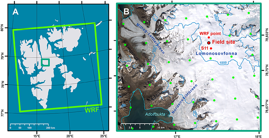
Figure 1. (A) Svalbard archipelago, large green polygon shows the extent of WRF domain, smaller dark-green polygon marks the area shown in (B). (B) Lomonosovfonna and its outlet glaciers. Green dots show locations of the WRF domain nodes; large red dot marks location of the AWS and thermistor strings (detailed sketch of installation is found in Marchenko et al., 2017: thermistor strings were installed in boreholes 1–9); smaller red dots show the WRF domain node, output for which was used to force the surface energy balance model and location of the stake S11. Background - true color satellite image LANDSAT ETM+ from 13 July 2002, contour lines and coastline data is provided by the Norwegian Polar Institute.

The study site is in the accumulation zone of the Lomonosovfonna ice field on a flat spot at 78.824°N, 17.432°E, 1,200 m a.s.l., well above the equilibrium line, which for Nordenskiöldbreen was estimated to be at 719 m a.s.l. (Van Pelt et al., 2012). The local glacier thickness derived from a GPR survey is 192 ± 5.1 m (Pettersson, 2009, unpublished data) and the thickness of the firn layer according to coring results was around 20 m in 2009 (Wendl, 2014). Recent modeling results in the area showed that at the elevation of our study site the melt rate during 1989–2010 was on average ≈0.34 m w.e. yr⁻¹ (Van Pelt et al., 2012). Accumulation at Lomonosovfonna is affected by the wind drift (Pälli et al., 2002; Van Pelt et al., 2014) and measured rates range between 0.58±0.13 and ≈0.75 m w.e. yr⁻¹ (Van Pelt et al., 2014; Wendl et al., 2015). Subsurface temperature measurements at Lomonosovfonna during summer season were carried out in 1965 (Zinger et al., 1966), 1980 (Zagorodnov and Zotikov, 1980), and more recently by Marchenko et al. (2017). While in Marchenko et al. (2017) the focus was on subsurface density and stratigraphy, in this study the analysis concentrates on the subsurface temperature evolution.

3. Data

3.1. AWS and Stake Measurements

For monitoring of the surface energy and mass fluxes an automatic weather station (AWS) was installed at Lomonosovfonna in April 2013 and reinstalled in April 2014 and 2015. Air temperature was measured every 3 h during 23 April–17 August in 2013 and 29 April 2014–1 May 2015. Downwelling and upwelling fluxes of short- and long-wave radiation (SW↓, SW↑, LW↓, LW↑, respectively) were measured every 30 min and averaged values were recorded every 3 h during 23 April–14 July 2013 and 28 April–26 August 2014. Details on the used instruments are given in the Table 1.

TABLE 1

Table 1. Instruments used for measurements of the air temperature, radiative energy fluxes, and subsurface temperature.

The AWS data were filtered to exclude potentially erroneous values from the analysis. Firstly, we discarded the values collected at battery voltage below the limits provided by the manufacturers of the corresponding instruments. Secondly, values outside of the feasible range were rejected: for air temperature this was <−40 and >10°C, for SW↓ and SW↑ this was <0 and >800 W m⁻² and for LW↓ <0 and >350 W m⁻². Additional constraints were also applied to LW↑ assuming that the glacier surface cannot be colder than −50°C and warmer than 0°C. The minimal (140 W m⁻²) and maximum (316 W m⁻²) values for the fluxes were calculated using the Stefan-Boltzmann law assuming a surface emissivity of 1, as:

$\begin{array}{l}LW\uparrow =\sigma ·T^4,\end{array}$

where σ = 5.67 · 10⁻⁸ Wm⁻² K⁻⁴ and T is the surface temperature in Kelvin. Radiation measurements are prone to significant biases due to deposition of rime on the sensors. Values possibly measured during periods dominated by riming were interpreted from occasional decreases in short wave radiative fluxes accompanied by a small difference between LW↓ and LW↑ and excluded from the analysis.

Measurements of snow depth and snow surface height at stake S11 during field campaigns in April 2012–2015 (Figure 1) are also used for validation of the simulated surface energy and mass fluxes. Although, the stake is situated at a distance of 1.5 km from our site, results from radar surveys (Van Pelt et al., 2014) suggest that there is no significant gradient in net annual accumulation rate between the two sites. Measurements at the stake yield estimates of accumulation during the period from August (when the summer surface is formed) to April and the net surface mass flux between two field campaigns. It has to be noted, that the measurements also include the effect of snow and firn settling. Winter accumulation rate measurements include the effect of snow settling that occurs above the previous summer surface and net annual accumulation measurements can be expected to be influenced by the gravitational densification occurring above the stake bottom. The latter can reach significant values as the in 2012 the stake bottom was at 8 m below the surface.

3.2. Snow and Firn Density

Firn density was measured in four cores drilled in April 2012–2014 by a Kovacs corer. The lengths of the cores were 9.9, 11.3 and 13.6 m. Details on the routines applied for extraction and processing of the cores were presented by Marchenko et al. (2017). For the further analysis the density profiles originally measured with a high vertical resolution were smoothed using a 1 m running average filter to exclude spikes caused by thin and likely not laterally consistent ice layers (Marchenko et al., 2017) and to ensure mass conservation.

3.3. Snow and Firn Temperature

Multiple thermistor strings were used to continuously record the evolution of the snow and firn temperature. In April 2012, 2013, and 2014 nine custom manufactured thermistor strings were installed in holes drilled by Kovacs auger with a 5.5 cm diameter. The depths of sensors on the strings are presented in Figure 2. The strings were installed in a 3 × 3 square grid pattern with 3 m separation between neighboring holes. To minimize preferential percolation of melt water along the cables, the holes were backfilled with drill chips and surface snow.

FIGURE 2

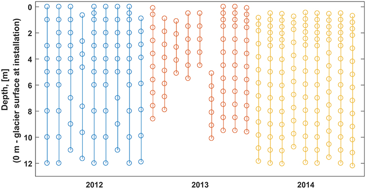
Figure 2. Depths of thermistors installed in April 2012 (blue), April 2013 (red), and April 2014 (yellow) referenced to the glacier surface at installation.

Each thermistor was connected in series with a reference temperature stable resistor to form a resistive half bridge. Precisely measured excitation voltage was applied to the circuit and the voltage drop over reference resistor was measured using a data logger. To increase the number of channels scanned by the logger several relay multiplexors were connected to it. Details on the applied electrical schemes are listed in the Table 1. During post-processing the voltages measured by the data logger were first converted to resistances and then to temperature values using the manufacturer guidelines.

The resulting datasets span the periods 22 April–9 October in 2012, 23 April–12 July in 2013, and 17 April 2014–11 April 2015. Time gaps between the periods covered by subsurface temperature monitoring are explained by the technical problems that occurred during summer 2012 (rapid battery drainage) and 2013 (flooding of the equipment case by melt water). To facilitate the comparison of firn temperature measured by multiple thermistor strings the data from individual strings were first interpolated to a common depth grid using shape-preserving piecewise cubic interpolation. In the next step, the resulting datasets were horizontally averaged to obtain a more spatially representative dataset for each year. We also define three time intervals with rapid subsurface temperature changes subjectively estimated from the results of measurements and interpreted as being driven by the release of latent heat from refreezing water: 2 June–25 September in 2012, 3 June–12 July in 2013, and 4 July–21 September in 2014. These time intervals are used in the further analysis of field data and for its comparison with the model outputs.

4. Modeling

4.1. Regional Climate Model WRF

The Weather Research and Forecast (WRF) regional climate model (Skamarock et al., 2008) has been previously shown to successfully reproduce the evolution of meteorological parameters measured by weather stations in Svalbard (Claremar et al., 2012; Aas et al., 2015, 2016). WRF was forced by ERA Interim weather re-analysis data (Dee et al., 2011) with the spatial resolution of 0.75°, the sea surface temperature and sea ice data from the Operational Sea Surface Temperature and Sea Ice Analysis dataset (Donlon et al., 2012) with 0.05° resolution. We used the dataset on land terrain elevation from the US Geological Survey, while glacier mask was provided by the Norwegian Polar Institute (Nuth et al., 2010). The following modules were used in WRF: land surface scheme NOAH-MP (Niu et al., 2011), turbulence scheme MYNN-2.5 (Nakanishi and Niino, 2006), radiation parameterization RRTMG (Iacono et al., 2008), cumulus convection from Grell and Dévényi (2002) and the double-moment micro-physics scheme from Morrison et al. (2005). The WRF model was run for a domain covering almost the entire Svalbard archipelago (Figure 1A) on a spatial resolution of 5.5 km (Figure 1B). For the further analysis we used four WRF output variables for the domain point that is closest to our study site and lies at 1,053 m a.s.l. (Figure 1B). Air temperature and relative humidity, precipitation and fractional cloud cover accounting for the presence of clouds in all atmospheric levels produced by WRF at 3 h temporal resolution serve as input for the coupled surface energy balance–firn model described below. Despite an elevation difference between the observation site and the model grid point of around 150 m a negative air temperature bias with respect to AWS measurements was found. However, no lapse rate based correction is applied as further discussed in Section 5.1.

4.2. Coupled Surface Energy Balance - Firn Model

To simulate the evolution of the surface and subsurface energy and mass fluxes we apply a model previously used for glaciers on Svalbard (Van Pelt et al., 2012, 2014; Van Pelt and Kohler, 2015). The model consists of two parts describing processes at and below the surface. The surface scheme developed along the lines of Klok and Oerlemans (2002) describes the energy and mass fluxes at the glacier surface and solves for the skin temperature, melt rate, and accumulation. The one dimensional subsurface scheme is based on the model presented by Greuell and Konzelmann (1994) modified by Reijmer and Hock (2008) and Van Pelt et al. (2012) to incorporate updated physics of liquid water storage, gravitational compaction, and heat conduction.

4.2.1. Surface Energy and Mass Fluxes

The surface scheme accounts for the following mass fluxes at the surface: accumulation due to solid precipitation and riming and mass loss due to melt and sublimation. The energy fluxes (in W m⁻²) at the surface are described by the equation:

$Q_m=S{W}_{net}+L{W}_{net}+Q_s+Q_{lat}+Q_{rain}+Q_{sub},$

where Q_m is the energy available for melt, SW_net and LW_net are the short and long wave radiation balances, respectively, Q_s and Q_lat are the sensible and latent turbulent heat fluxes, Q_rain is the energy supplied by rainfall, Q_sub is the subsurface conductive heat flux. Detailed information on the formulations for individual energy fluxes can be found in Klok and Oerlemans (2002) and Van Pelt et al. (2012) and references therein.

On each time step the surface energy balance scheme estimates the above listed fluxes and solves for the surface temperature. In case the resulting value exceeds 0°C, it is reset to ice melt temperature and the fluxes dependent on surface temperature (LW_net, Q_s, Q_lat, and Q_sub) are recomputed to produce the Q_m.

4.2.2. Firn Model

At each time step the subsurface model simulates temperature (T, °C), density (ρ, kg m⁻³) and “wet” gravimetric water content (θ_w = m_w/m_tot, grav.%, where m_w is the mass of water and m_tot is the total mass) of multiple snow, firn and ice layers. The model uses a moving grid in which the boundaries between layers are kept constant over time (Lagrangian scheme). That allows to take into account the effects of vertical advection of snow and firn layers with respect to the surface induced by mass fluxes at the surface. Gravitational settling of the layers is described following Ligtenberg et al. (2011): density of the layers increases with time as a function of the accumulation rate and local subsurface temperature. Conductive heat exchange in the profile is described by the Fourier's law with the conductivity of individual layers parameterized as a function of their density following Calonne et al. (2011). It is assumed that at the lower boundary of the model domain the heat flux equals zero. Although, the simulations are performed for a ca. 25 m thick domain, the output only for the upper 12 m is analyzed in detail, as the vertical extent of the empirical dataset on subsurface temperature and density is limited.

Refreezing of surface liquid water strongly influences the subsurface conditions. The routines applied to describe the processes at each time step of the model are described in Figure 3. The original subsurface scheme is built following the widely applied “bucket” approach and is referred to below as the “default water infiltration scheme.” According to it all water is first allocated to the topmost layer after which its downwards propagation is estimated. Water is allowed to advance to the underlying layer when the refreezing capacity (RC in Figure 3) of the current one is eliminated and the gravimetric water content exceeds the maximum gravimetric water content (or water holding capacity—WHC in Figure 3) — potential of capillary and adhesive forces to retain water against gravity. Water holding capacity of snow and firn is parameterized as a function of density following Schneider and Jansson (2004) and decreases from 11 to 2 grav.% with the density rise from 350 to 900 kg m⁻³. Temperature and density of subsurface layers changes in response to the refreezing of water. The model also describes buildup of slush water layer on top of the lowermost solid ice layer that is assumed to be impermeable and superimposed ice formation as a result of freezing of the slush layer. However, in our case no slush water is generated in the upper 15 m as density never reaches the density of ice there. Runoff is possible either from the bottom of the domain or from the slush layer as a function of time (Zuo and Oerlemans, 1996).

FIGURE 3

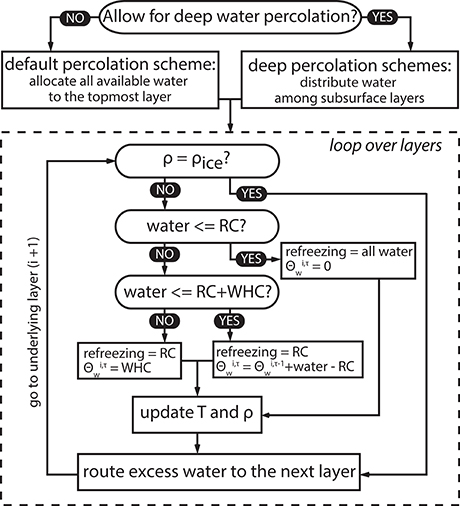
Figure 3. Schematic diagram illustrating routines executed to assess the influence of liquid water refreezing on the temperature (T), density (ρ), and water content (θ_w) of subsurface layers at one time step (τ). RC, refreezing capacity defined by the layer's temperature and density; WHC, water holding capacity defined by the potential of capillary and adhesive forces to retain water within a layer against gravity.

4.2.3. Deep Water Infiltration Schemes

Motivated by previous studies pointing to the highly inhomogeneous pattern of water flow in snow (e.g., Williams et al., 2010) and associated uncertainties in simulating the subsurface mass and energy fluxes (e.g., Gascon et al., 2014; Langen et al., 2017; Steger et al., 2017) we implement different parameterizations of the deep water percolation in snow and firn. Preferential water flow essentially concentrates water flow at certain parts of the snow and firn profile even if water supply at the surface exhibits no lateral variability (e.g., Katsushima et al., 2013). This effect is schematically illustrated by Figure 4A, which, however, is not based on field or simulation data. In a horizontally averaged 1-D case the phenomena can be expressed by allowing fractions of surface water to penetrate to different depths.

FIGURE 4

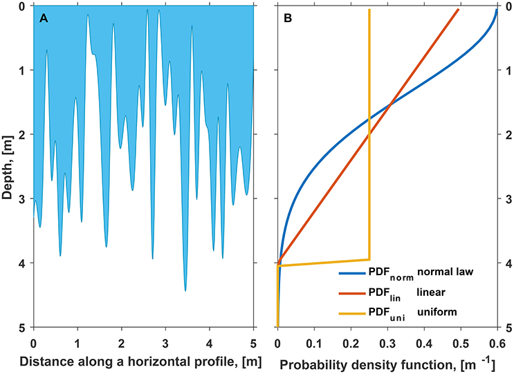
Figure 4. (A) A schematic representation of preferential water flow in a snow and firn pack - blue color shows the wet part of an imaginative snow pit wall. Vertical and horizontal scales and the shape of the “wetting front” are chosen arbitrarily for illustrative purposes. (B) Probability density functions corresponding to the deep water infiltration schemes implemented in the firn model. Values along the horizontal axis can also be interpreted as the fractions of surficial water that would be allocated to a 1 m thick firn layer found at a specific depth.

In each model time step the mass of liquid water available at the surface is distributed among the subsurface layers before the effect of refreezing is assessed (Figure 3). The distribution is governed by a probability density function PDF(z, z_lim), where argument z (m) is depth and z_lim (m) is the single tuning parameter—the depth below which no (or only a small fraction) liquid water is allocated. Since liquid water is generated at the surface it was assumed that deeper layers generally receive less water and the PDF(z, z_lim) function decreases with depth. We test three different implementations of this probabilistic approach with different shapes of the PDF(z, z_lim) function. Corresponding curves are presented in Figure 4B. In contrast to the default infiltration scheme, the tested deep percolation routines allow for instantaneous percolation below 0°C level, thereby mimicking the effect of piping at the lateral scale of several meters.

Uniform water infiltration scheme (yellow curve in Figure 4B) assumes that water is equally distributed above z_lim and no water is allowed to infiltrate below this level:

$PD{F}_{uni}(z,z_{lim})=\{\begin{array}{cc}\frac{1}{z_{lim}},\hfill & \mathrm{\text{if}}z<z_{lim}\hfill \\ 0,\hfill & \mathrm{\text{otherwise}}\end{array}$

According to the linear water infiltration scheme (red curve in Figure 4B) the PDF(z, z_lim) function decreases with depth at a constant rate and reaches 0 at z_lim:

$PD{F}_{lin}(z,z_{lim})=\{\begin{array}{cc}\frac{2(z_{lim}-z)}{z_{lim}^2},& \mathrm{\text{if}}z<z_{lim}\hfill \\ 0,\hfill & \mathrm{\text{otherwise}}\end{array}$

The normal law water infiltration scheme (blue curve in Figure 4B) distributes the water mass according to the corresponding probability density function with the standard deviation σ = z_lim/3, implying that 99.7% of the water stays above z_lim:

$PD{F}_{norm}(z,z_{lim})=2\frac{exp(-\frac{z^2}{2{\sigma }^2})}{\sigma \sqrt{2\pi }},$

Thus with the same z_lim value the relative amount of surficial water allocated to the firn layers just above z_lim is maximum for the uniform infiltration scheme and minimal for the normal-law percolation. Using the above defined PDF(z, z_lim) functions we estimate the fraction of the surface water that is added to subsurface layer i with thickness dz_i as:

$k^i=PDF(z_i,z_{lim})·d{z}_i.$

The suggested schemes describing deep water percolation do not incorporate the physical details of the water transport processes occurring in snow and firn but are rather a statistical description of the horizontally-averaged effect of deep percolation on firn conditions at the scale of several meters. Although, we optimize the model to minimize the mismatch with the averaged temperature evolution measured on a 6 × 6 m plot, the results may also be useful for larger scale applications.

4.3. Model Setup

We set the values of the tuning parameters in the surface energy balance scheme such as the aerosol transmissivity exponent, emissivity exponent at clear-sky and overcast conditions, turbulent exchange coefficient following Van Pelt et al. (2012), who carried extensive calibration experiments at Nordenskiöldbreen and Lomonosovfonna using the data from an AWS at 600 m a.s.l. and readings at multiple stakes. In line with Van Pelt et al. (2014) the value of the fresh snow albedo was set to 0.89, which also resulted in best fit between the simulated and measured LW↑.

The coupled energy balance-firn model was run for a single point at the study site (Figure 1B) with a 3 h temporal resolution during 1 April 2012–1 May 2015. The subsurface scheme is based on a one-dimensional vertical domain comprising 250 layers with an initially uniform thickness of 0.1 m. The firn model is initiated by the temperature and density profiles measured in April 2012. On the 23^d and 18^th April 2013 and 2014, respectively, the simulated density and temperature distributions are reset to the values measured on the corresponding dates to minimize cumulative errors. The gravimetric liquid water content in the profile is reset accordingly to ensure that no liquid water is present in layers at subfreezing temperature.

To explore the effect of deep water percolation on the simulated snow and firn temperature evolution the infiltration schemes described in Section 4.2.3 were implemented and tested for a range of z_lim values: 0.1 m and 0.5–25 m with a step of 0.5 m. We also investigate the model response to perturbation of the surface energy balance by an additional term E₊ set to −5 and 5 W m⁻², which corresponds to a ca. 22% decrease and a ca. 27% increase in surface melt rate, respectively. For the default infiltration scheme additional experiments were also performed for a range of E₊ values up to 50 W m⁻².

5. Results

5.1. Surface Energy Fluxes

The simulated surface conditions at Lomonosovfonna are validated by comparing the output of the WRF model and of the surface energy balance scheme with the AWS and stake measurements. The measured and simulated evolution of air temperature is presented in Figure 5. The modeled mean annual temperature at the study site during April 2012–April 2015 is −11.7°C and shows a pronounced seasonal cycle. In summer months the temperature reaches a few degrees above zero while during cold spells in winter it can drop down to −30°C (Figure 5A). The WRF model reproduces well the observed air temperature (Figure 5B, Table 2) with a root mean square difference (RMSD) of just below 2°C and an underestimation by −0.44°C averaged over the period of observation.

FIGURE 5

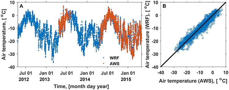
Figure 5. Air temperature at the Lomonosovfonna ice field in April 2012–2015. (A) Values simulated using the regional climate model WRF (blue), AWS measurements (red). (B) Scatter plot illustrating the agreement between the simulated and measured values.

TABLE 2

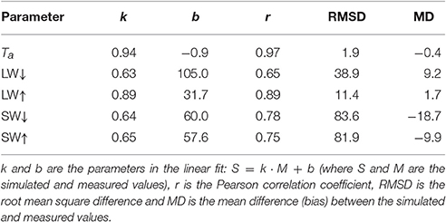
Table 2. Model performance in reproducing the air temperature (T_a) and radiative fluxes measured at the AWS (see Figures 5, 6).

Agreement between the simulated and measured radiative energy fluxes is illustrated by the scatter plots in Figure 6. The mean deviation and RMSD values between the measured and modeled LW↓ values are 9 and 39 W m⁻², respectively (Table 2). The cloud of points in Figure 6A describing the model performance in reproducing the LW↓ can visually be divided into three parts. The points lying along the diagonal line correspond to a good match between the measured and simulated values, while the points occurring above and below the diagonal line indicate respectively over- and under-estimation of the energy flux by the model. Since, the LW↓ flux is heavily dependent on the cloud cover (e.g., Klok and Oerlemans, 2002; Stephens, 2005), we suggest that the three clusters of points are respectively explained by: small errors, over- and underestimation of the cloud cover (n) by the WRF model.

FIGURE 6

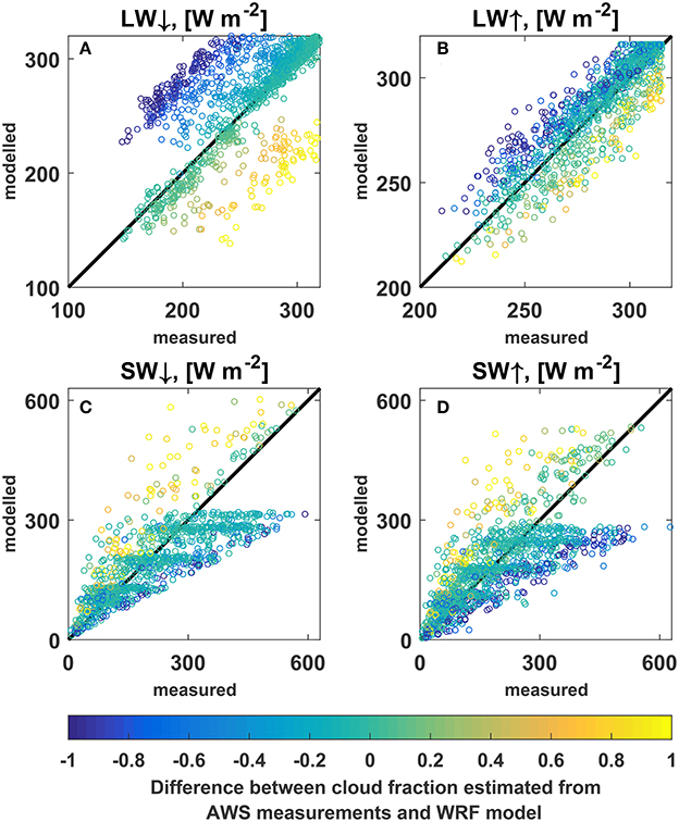
Figure 6. Scatter plots illustrating the agreement between the measured and simulated intensities of the radiative energy fluxes at the Lomonosovfonna ice field during 23 April–14 July 2013 and 28 April–26 August 2014. (A) Long wave downwelling radiation. (B) Long wave upwelling radiation. (C) Short wave downwelling radiation. (D) Short wave upwelling radiation.

This interpretation of LW↓ scatter plot (Figure 6A) is supported by an independent estimation of the n values based on the LW↓ and air temperature measurements at the AWS following the approach of Kuipers Munneke et al. (2011) which assumes a linear dependence between these two parameters for any given air temperature. The resulting differences between the AWS-estimated and WRF-predicted cloud cover fractions are shown as the color code of points in Figure 6. Overestimation of the cloud cover by the WRF model indeed results in artificially high LW↓ values and occurs more often than underestimation. The upper cluster of points in Figure 6A is significantly larger than the lower and the mean cloud cover fraction estimated from the LW↓ and air temperature measurements is 0.65, while the average of WRF derived values for the same period is 0.85.

The mean differences between the simulated and measured short wave radiative flux values (Figures 6C,D; Table 2) are −19 and −10 W m⁻² for the downwelling and upwelling components, respectively, although RMSD are considerably larger and are above 80 W m⁻². We also find that the mean daily albedo (i.e., the averaged relation between mean daily SW↑ and SW↓ values) produced by the model (0.88) is significantly higher than the corresponding measured value (0.80), which is most probably explained by the measurement uncertainties related to the tilt of the AWS mast and riming of sensors. Overestimation of the cloud cover in the forcing data results in reduced SW↓ values, while when the WRF model underestimates the cloud cover, SW↓ is too high (Figure 6C).

The negative effect of the overestimated cloud cover on SW↓ is more than compensated by the positive effect on the LW↓. Figure 7 illustrates the cumulative melt produced by the model during the 3 year period. It is apparent that the model forced by overall lower n values based on AWS measurements, when those are available, produces significantly less melt water compared to the reference run done using the cloud cover from WRF (solid red and blue curves on Figure 7 correspondingly). The effect is also seen in Figure 6B illustrating the agreement between measured and simulated LW↑: overestimation of cloud cover by WRF also results in higher simulated LW↑ values than measured by the radiometer (blue points).

FIGURE 7

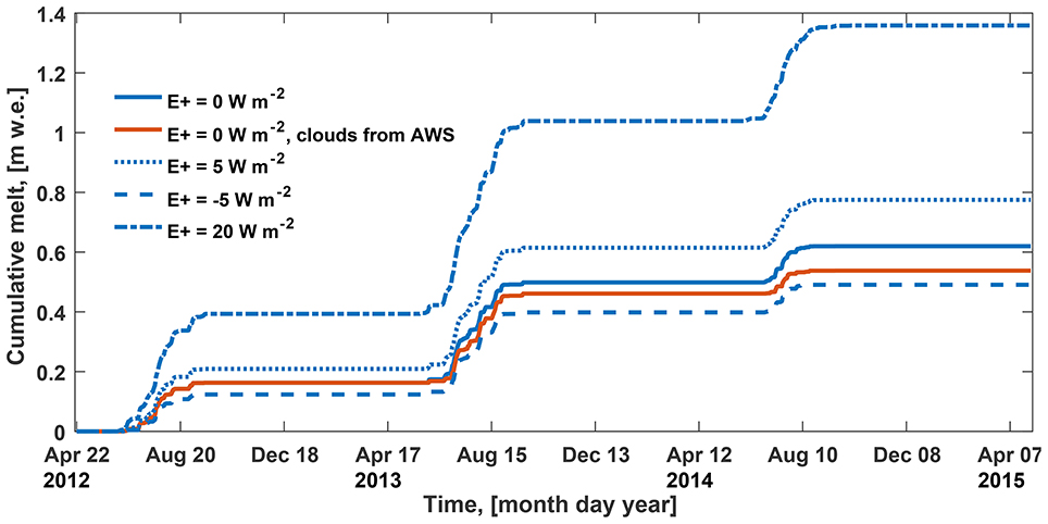
Figure 7. Simulated cumulative melt rate at the Lomonosovfonna ice field in April 2012–2015 for different forcings and settings of the energy balance scheme. Blue lines are used when cloud forcing is provided by WRF, red - cloud forcing is approximated following Kuipers Munneke et al. (2011) using AWS measurements of LW↓ and air temperature, when those are available, when not WRF output is used.

The upwelling long wave radiative energy flux appears to be in close agreement with the measurements (Figure 6B, Table 2). LW↑ is a function of the surface temperature and is defined by the sum of all energy fluxes at the surface. High correlation (0.89) between the modeled and measured LW↑ (Table 2) hence suggests the high accuracy of simulated surface temperature, timing of melt events and also of the melt rate, assuming that the physics of energy fluxes above subfreezing and melting surfaces are similar. In absence of data to directly validate melt rate at the site this provides an important indirect source of validation of simulated melt rates. The absence of a clear bias in simulated surface temperature can be ascribed to compensating effects of the uncertainties in simulated cloud cover (overall positive), air temperature and surface albedo (negative), and turbulent fluxes.

The average winter (ca. August to April) and annual surface height change measured at stake S11 in April 2012–2015 is 1.8 and 1.3 m correspondingly. The average simulated surface height change during the period starting at the surface's lowermost position in July–September (12, 8, and 26 August 2012, 2013, and 2014) and ending at the day when the stake is revisited in April next year is 1.7 m. Estimation of snow gravitational settling during the time following Ligtenberg et al. (2011) yields ca. 0.1 m and thus the surface height change is reduced to 1.6 m. The average annual increment in the surface height during April 2012–April 2015 is 1.7 m. If snow and firn settling above the layer that in April 2012 is at the depth of 8 m (stake length below the surface) is taken into account following Ligtenberg et al. (2011) the value decreases to 1.3 m. The close agreement between modeled and observed dynamics of the surface height suggests decent performance of the surface scheme forced by the WRF model output in reproducing the energy and mass fluxes at our field site on Lomonosovfonna.

The amount of melt water produced by the reference run of the model (blue solid curve in Figure 7) in 2013 (0.34 m w. e.) is significantly larger than in 2012 (0.16 m w. e.) and in 2014 (0.12 m w. e.). This finding agrees with glacier-averaged stake mass balance data for Nordenskiöldbreen (unpublished data described in Van Pelt et al., 2012) according to which the summer mass balance in 2012, 2013, and 2014 was −0.37, −0.79, and −0.35 m w.e., respectively.

5.2. Observed Snow and Firn Temperature Evolution

The measured snow and firn temperature evolution averaged over all thermistor strings installed in each of the field campaigns is presented in Figure 8A. The vertical depth scale is corrected using the modeled change in the surface height and thickness of subsurface layers to account for the accumulation and ablation at the surface and gravitational settling below it.

FIGURE 8

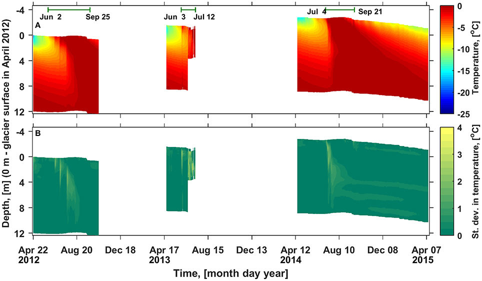
Figure 8. Evolution of the snow and firn temperature measured at the Lomonosovfonna ice field in April 2012–2015. The depth scale was corrected using the model output to account for the accumulation/melt at the surface and gravitational settling below it. (A) Temperature values interpolated to a finer mesh (0.1 m between grid nodes) and averaged over all thermistor strings installed in each of the field campaigns. Green bars in the upper part of the panes mark the time intervals used in calculations presented in Figures 9, 11. (B) Evolution of the standard deviation in snow and firn temperature at one depth used here as a measure of the horizontal temperature gradients.

In April of each year temperature increases from ca −15°C at the surface to 0°C at ca 10 m depth (Figure 8A). Data from June and July 2012 and 2013 shows that warming of the profile occurred in several steps associated with events of intensive melt at the surface (Figure 7). The entire profile was temperate by August 24 in 2012 and by August 9 in 2014. Data for the later part of the summer season in 2013 is not available, however, considering the high melt rates simulated for that year (Figure 7), it can be expected that the upper 12 m of the firn profile became temperate even earlier than in the other two years. Snow and firn temperature evolution during the autumn and winter months was only measured in 2014. It is apparent that in the absence of surface melt starting from the first days of September, the layer of temperate snow and firn is eliminated due to the conductive heat flux toward the cooling surface.

To characterize the lateral variability of the snow and firn temperature measured simultaneously at the same depth standard deviations for corresponding sets of values from multiple thermistor strings were calculated (Figure 8B). The standard deviations reach up to 4°C and during all three melt seasons the areas with increased lateral variability in snow and firn temperature descend to greater depth over time following the 0°C isotherm, where intensive refreezing can be expected. The observation can be related to the horizontal gradients in the rate of downward water flux and associated migration of maxima in lateral temperature variability. It is particularly obvious during the ablation season in 2012, when the melt water generated at the surface during the first warm spell on the 20th June reached no deeper than 2 m, while the consecutive ablation events on the 4th and 23rd July likely brought the water deeper: to 5 and 9 m at maximum, respectively. In 2014 increased lateral variability in snow and firn temperature is also observed during the autumn and winter months at 4.2, 6.3, and 8.5 m (Figure 8). Referenced to the glacier surface in April 2014 these depths correspond to 7, 9.1, and 11.3 m. The phenomena can be related to perched horizons with increased water content that have a horizontal extent less than the plot covered by our thermistor measurements (6×6 m). In April 2014 Marchenko et al. (2017) found multiple ice layers at 7, 8, 9, and 10.8 m depth in three boreholes where the thermistor strings used in present study were installed afterwards. These ice layers could have acted as impermeable horizons and retained water which locally inhibited the cold wave penetration.

The occasional high lateral temperature gradients during the 3 years of observations at Lomonosovfonna indicate a possible uncertainty in subsurface temperature measurements performed at single locations in accumulation zones of glaciers. Higher values of the standard deviations (Figure 8B) during the summer period suggest that the largest uncertainty can be expected during liquid water infiltration in the snow and firn. Data from multiple thermistor strings installed in close vicinity of each other and monitored simultaneously during three melt seasons allows to investigate the effect of averaging the measured temperature evolution over a varying number of thermistor strings.

Firstly for each of the three periods with rapid subsurface temperature changes (see the green bars in Figure 8A) a reference dataset was defined as an average of all nine thermistor strings available (N_strings = 9). Secondly, multiple sample datasets were constructed by averaging data from N_strings = 1…9 thermistor strings. The resulting average RMSD between the reference and the samples are presented in Figure 9. For the 2012 and 2014 datasets the RMSD value decreases from ≈0.4°C for single thermistor string to ≈0.25°C for 3 strings, while the RMSD for larger N_strings values decrease at a slower rate. For the dataset collected in 2013 the RMSD values also show a decrease with the number of strings but the values are generally higher and the concave pattern in lacking. We relate these observations to the shorter period of measurements and a lesser number of thermistors scanned during the season (see Figure 2) and note that the subsurface temperature dataset collected during 2013 is the most uncertain. Thus it becomes apparent that monitoring the summer evolution of subsurface temperature using multiple thermistor strings is beneficial as the resulting laterally averaged dataset is more representative for the study site.

FIGURE 9

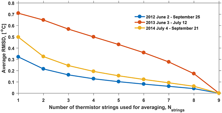
Figure 9. Sensitivity of the measurements of subsurface temperature evolution during the summer period to the number of thermistor strings (N_strings) expressed as the averaged RMSD between the reference dataset (N_strings = 9) and averages of different number of thermistor strings (N_strings = 1…9).

5.3. Modeling Snow and Firn Temperature Evolution

Figure 10 presents the evolution of snow and firn temperature simulated with E₊ = 0 W m⁻² and using the conventional water percolation scheme not allowing for deep water infiltration (Figure 10A) along with the corresponding deviations from the measurements (Figure 10B) and simulated gravimetric water content (Figure 10C). The general pattern of subsurface temperature evolution agrees with the results of measurements. In May and June a gradual warming occurs due to the increase of air temperature. Between mid-June and July infiltrating water causes a fast downward expansion of the temperate snow and firn layer. Evolution of the water content profile follows the firn temperature changes: water saturates the potential of the capillary and adhesive forces immediately after the layer in question becomes temperate. In September, after surface melt ceases, the subsurface profile gradually cools, and the water suspended in pores is refrozen. The temperature below ≈10–12 m remains always at 0°C, it is set to the observed state every April and the conductive cold wave does not reach that deep during 1 year.

FIGURE 10

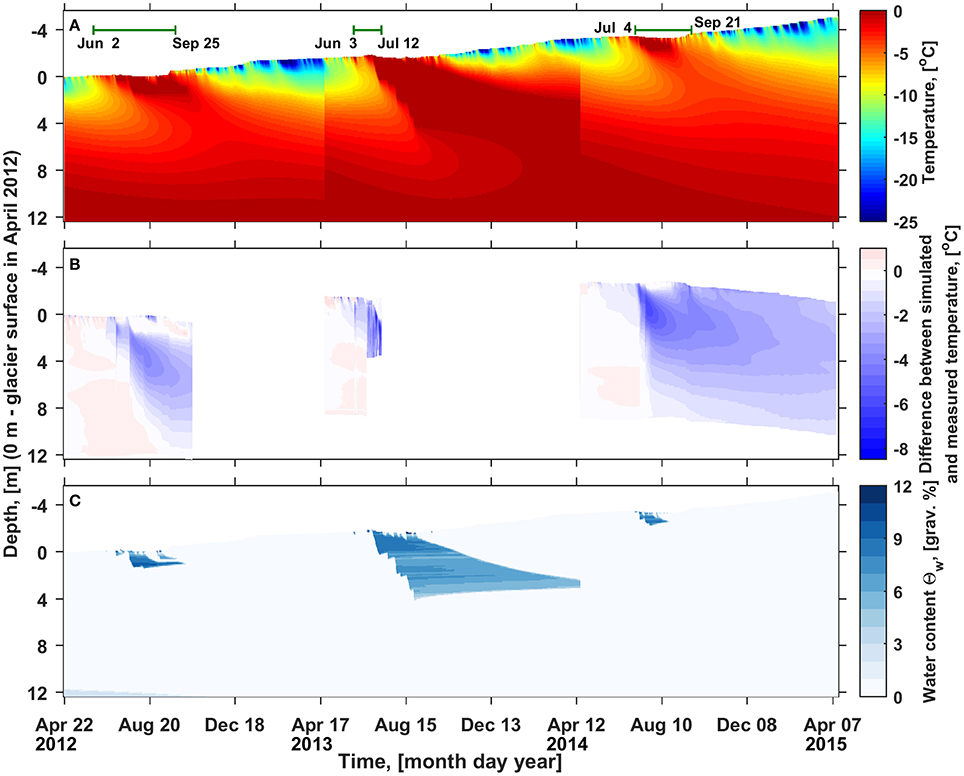
Figure 10. (A) Evolution of the snow and firn temperature simulated using E₊ = 0 W m⁻² and the default water infiltration scheme. Green bars in the upper part of the panel mark the time intervals used in calculations presented in Figure 11. Resetting the simulated temperature profile to the measured values on the 23rd, 18th, and 16th April 2013, 2014, and 2015, respectively causes the sudden shifts in temperature evolution. (B) Difference between the simulated (A) and measured (Figure 8A) temperature evolution. Values larger than 1°C constitute ca 0.33% and are shown as 1°C. (C) Evolution of the simulated gravimetric water content (Θ_w)

Despite the general agreement between the simulated and measured subsurface temperature, the vertical extent and strength of perturbations in the snow and firn temperature deviate considerably from the observations (Figure 10B) with the simulated profile being generally colder. The difference between the simulated and measured temperature reaches up to 12.5 and −8°C. While only 0.3% of the RMSD values are >1°C, 42.3% of the deviations are below −1°C. Biases are the largest in July, when high surface melt rate results in fast and deep water infiltration, which is not captured by the firn model in its default configuration. Positive errors in simulated temperature occur very seldom and are restricted to the upper 1 m of the profile. We note that the depth of elevated negative anomalies increases over time as the deeper firn layers become temperate under the influence of infiltrating water. By the end of all three simulated ablation seasons the subsurface profile did not reach the temperate state. Cold firn was still present below 2 m depth in 2012 and 2014, and below 6.5 m in 2013, when the surface melt rate was higher and the temperate near-surface firn layer almost connected with the deep temperate firn.

Next we explore the sensitivity of the firn model results to different water infiltration schemes and the value of the percolation depth z_lim. The RMSD between simulated and measured subsurface temperature during the periods of rapid changes (Figure 11) is 1.5–2.8°C for the default infiltration scheme and all three deep infiltrations schemes with z_lim set to 0.1 m. With the increase of z_lim to 25 m the RMSD values in all cases exhibit a gradual decrease approximately by a factor of 2 and a subsequent increase almost to the initial values. The presence of a minimum in each case suggests that implementation of the deep water percolation scheme significantly improves the firn model performance in reproducing the measured subsurface temperature evolution. The z_lim values corresponding to the minimal RMSD between the simulated and measured temperature evolution lie in a wide range from 4.5 to 12 m for different years and parameterizations, with a consistent pattern of the uniform percolation exhibiting the smallest values (4.5–6 m) and the normal law percolation the largest (7.5–12 m). At the same time, the minimal RMSD values reached for the different infiltration schemes vary only slightly.

FIGURE 11

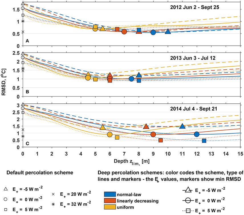
Figure 11. Sensitivity of the RMSD between the simulated and measured summer subsurface temperature on the type of the infiltration scheme, depth z_lim to which liquid water is allowed to infiltrate and parameter E₊ regulating the energy available for melt. (A) 2 June–25 September 2012; (B) 3 June–12 July 2013; (C) 4 July–21 September 2014. Note the difference in the limits of the vertical axis. Black markers in each panel show the RMSD for the default water infiltration scheme, blue color shows the results for “normal law,” red for the “linear” and yellow for the “uniform” infiltration laws. Markers show location of the minima in RMSD for each of the RMSD = f(z_lim) functions. Type of the line and marker code tuning of the surface energy balance model: solid lines and circles for E₊ = 0 W m⁻², dashed lines and triangles for E₊ = −5 W m⁻² and dotted lines and squares for E₊ = 5 W m⁻².

Sensitivity experiments for the default configuration of the firn model revealed that decreasing the amount of melt (E₊ = −5 W m⁻²) results in slightly higher values of the RMSD between the simulated and measured temperature evolution. Higher melt rates (E₊ > 0 W m⁻²) improve the model performance (Figure 11). While a moderate perturbation of E₊ = 5 W m⁻² results only in a slight reduction of the RMSD, with significantly higher E₊ values it is possible to reach a similar effect as by implementation of the deep percolation schemes. However, that is only possible with E₊ = 20 W m⁻² in 2012, E₊ = 22 W m⁻² in 2013, and E₊ = 32 W m⁻² in 2014, which corresponds to increase in the annual melt amount by a factor 2.2, 1.9, and 4.2 for the 3 years, respectively. Given the above described model performance in reproducing the observed energy and mass fluxes at the surface the major underestimation of melt rates seems unrealistic.

In most cases for any given z_lim value in the deep infiltration schemes setting E₊ to −5 W m⁻² (dashed lines) results in the highest RMSD values, while E₊ = 5 W m⁻² (dotted lines) leads to the minimal errors. However, the minimal RMSD values obtained with different settings of E₊ for the deep percolation schemes exhibit this dependence only in 2014, while in 2012 and 2013 the performance of the firn model depends only slightly on the settings of the surface melt rate.

Figure 12 presents the snow and firn temperature evolution simulated using E₊ = 0 W m⁻² and the uniform law percolation scheme with z_lim=5 m, which is the average of the three z_lim values resulting in minimal RMSD for that scheme in 2012, 2013 and 2014. The misfit between the simulated and measured temperature evolution (Figure 12B) still reaches −8 and 12.5°C, but the corresponding time and depth ranges are rather limited. Only 2.3% of the values are >1°C and 13.6% are below −1°C, which is much lower than what was produced by the firn model in its default configuration (Figure 10B). A notable overestimation of the firn temperature occurs in July 2012, while in the other two seasons firn temperature is slightly underestimated. The firn profile reaches the temperate conditions by the end of ablation seasons in 2012 and in 2013 in line with the observations. However, in summer 2014 increase of the deep firn temperature remains underestimated. A better match is found with E₊ set to 5 W m⁻² (blue square in Figure 11C) but a considerable cold firn layer is still present by the end of ablation season, suggesting that simulated melt rates are likely underestimated during this ablation period. The firn gravimetric water content (Figure 12C) follows the downwards propagation of the 0°C level but is considerably lower than in the case of default water percolations scheme (Figure 10C). The density profile is similar in both model realizations, suggesting no difference in the maximum gravimetric water content, and, consequently, significantly lower saturation values in case deep water percolation is assumed.

FIGURE 12

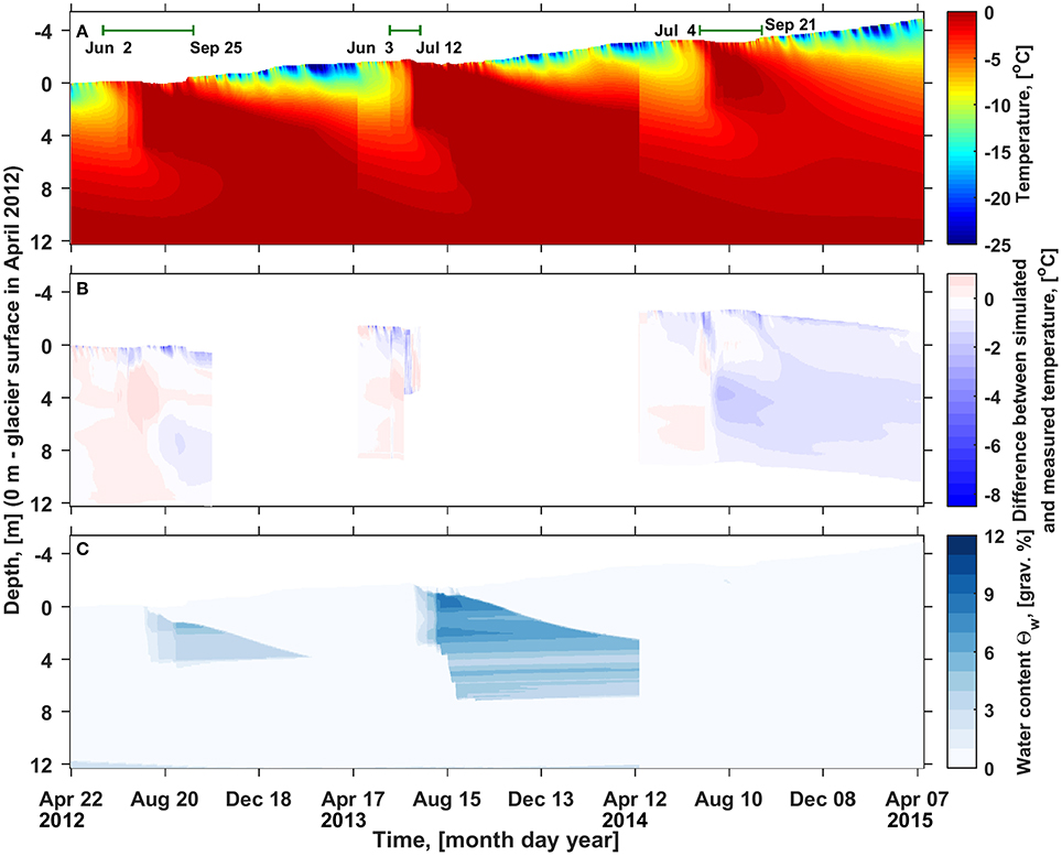
Figure 12. (A) Evolution of the snow and firn temperature simulated using E₊ = 0 W m⁻² and the uniform law water infiltration scheme with z_lim=5 m, corresponding to the average of z_lim values resulting in minimal RMSD for the summer seasons 2012 – 2014. Green bars in the upper part of the panel mark the time intervals used in calculations presented in Figure 11. Resetting the simulated temperature profile to the measured values on the 23rd, 18th, and 16th April 2013, 2014, and 2015, respectively causes the sudden shifts in temperature evolution. (B) Difference between the simulated (A) and measured (Figure 8A) temperature evolution. Values larger than 1°C constitute ca 2.3% and are shown as 1°C. (C) Evolution of the simulated gravimetric water content (Θ_w). Note: the color scales are the same as in Figure 10.

6. Discussion

The air temperature simulated by WRF for the point at 1053 m a.s.l. is on average 0.4°C lower than the values measured by the AWS at 1,200 m a.s.l. even though an opposite tendency can be expected from the elevation difference of ≈150 m and published lapse rate values for Svalbard of 4–6.6°C km⁻¹ (Wright et al., 2005; Nuth et al., 2012). Given the high correlation coefficient (0.97, see Table 2) between the measured and modeled values we conclude that in accordance with earlier results from Svalbard (Claremar et al., 2012; Aas et al., 2015, 2016) the WRF model demonstrated a prominent skill in reproducing the observed air temperature with a tendency for its underestimation.

The cloud cover generated by WRF clearly exceeds the approximations based on the AWS measurements of LW↓ and air temperature following Kuipers Munneke et al. (2011). In contrast with our findings, Aas et al. (2015) reported underestimation of the cloud optical depth at Ny Ålesund (20 m a.s.l.) and Etonbreen (370 m a.s.l., Austfonna). That inconsistency may be explained by the fact that our study site is at a considerably higher elevation.

We find that monitoring the evolution of subsurface temperature using multiple thermistor strings scanned simultaneously and installed in close vicinity from each other is advantageous. It allows to derive a more spatially representative dataset by averaging data from several strings. The latter is of particular relevance during the period of melt water infiltration occurring not homogeneously and resulting in the highest standard deviations in temperature measured at the same depth (Figure 8B). The shape of the RMSD = f(N_strings) function (Figure 9) suggests that representativity can be significantly improved by increasing the number of strings to 3 or 4. The typical values of RMSD between the reference and averages of different number of thermistor strings (Figure 9) are consistently and significantly lower than the RMSD between the simulated and measured subsurface temperature (Figure 11). This justifies utilization of the empirical data for constraining the suggested schemes describing deep water percolation and validating the modeling results. In a broader context it also proves the potential of temperature tracking of melt water in snow and firn packs (Conway and Benedict, 1994; Pfeffer and Humphrey, 1996; Humphrey et al., 2012; Cox et al., 2015; Charalampidis et al., 2016).

Subsurface temperature measurements at Lomonosovfonna provide evidence of warming that occurred during the last decades. The firn temperature measured at 10 m depth in August 1965 (Zinger et al., 1966, 1,050 m a.s.l.) and 1976 (Zagorodnov and Zotikov, 1980, 1,120 m a.s.l.) was in the range of −3 to −2°C and the seasonal temperate surface layer reached the maximum depth of 2–3 m. This suggests that the upper reaches of the ice field, at that time, belonged to the cold firn zone according to the classification of Shumskii (1964). However, our results show that by the end of the ablation seasons 2012–2014 the firn at Lomonosovfonna was temperate down to 10 m meaning that the study site is now in the warm firn zone and runoff may occur.

Reproducing these observations appears to be challenging for the firn model with the default configuration of the water infiltration scheme (Figure 10). By the end of all three ablation seasons the simulated subsurface profile still contained thick layers of firn at subfreezing temperature, which eliminates the possibility of runoff. Underestimation of the snow and firn temperature also results in errors in the simulated conductive heat flux below the surface and consequently biased estimations of other components of the surface energy balance. Additionally, a higher viscosity of too cold firn and ice (Cuffey and Paterson, 2010) may induce biases in long-term simulations of glacier dynamics.

Increasing the surface melt rate by 27% by setting E₊ to 5 W m⁻² resulted only in moderate decrease of the RMSD between the simulated and measured firn temperature and did not produce a warm firn pack by the end of ablation seasons 2012–2014. Larger perturbations (E₊ = 20, 22, and 32 W m⁻² in 2012–2014) significantly reducing the RMSD between the simulated and measured subsurface temperature evolution seem unlikely. Serious changes in the settings of the surface energy balance scheme result in reduction of the performance in validation of the model output against data from stake S11 and the AWS, particularly the LW↑ measurements. The spatial and temporal dynamics of the errors in simulated subsurface temperature evolution (Figure 10B) had the same principal characteristics as evolution of the standard deviations in temperature measured at the same depth (Figure 8B). Altogether this suggests that in conditions of short ablation period at Lomonosovfonna the latent heat of infiltrating and refreezing water heats up the subsurface profile more effectively than it is possible within the default infiltration scheme.

The tested deep percolation schemes allowed to significantly reduce the RMSD between the simulated and measured temperature evolution (Figures 11, 12B). The deep infiltration schemes result in more effective heating of the subsurface profile by the latent heat of refreezing water due to two mechanisms. Firstly, water going deeper releases latent heat at greater distance from the surface, where temperature gradients are low, and conductive heat exchange is not effective. At the same time, the upper part of the profile is allowed to maintain subfreezing temperature longer and by this be more readily warmed up by conduction from the melting surface. Secondly, by allowing a fraction of water to go past the upper firn horizons the potential of capillary and adhesive forces to retain some of the water in the upper layers is underused.

Two dimensional empirical data on the volumetric liquid water content of the seasonal snow packs presented by Techel and Pielmeier (2011) evidences that even though the source of liquid water is at the surface and the dominant flow is directed downwards, perched pockets with increased liquid water content can be present within snow pack along with pockets with reduced liquid water content. Thus the estimates of snow water holding capacity obtained by measuring the liquid mass retained by the sample after being entirely soaked and then drained (Coléou and Lesaffre, 1998; Schneider and Jansson, 2004) may be not immediately applicable in 1D snow and firn models at the onset of the water infiltration. Measurements of the volumetric water content in seasonal snow using upward directed radar conducted by Heilig et al. (2015) yielded the values of <2 vol.% at the onset of outflow from the snow pack registered by lysimeter. Converted to the relative gravimetric water content this corresponds to 6 grav.% assuming the density of 350 kg m⁻³, which is significantly lower than the 10.7 grav.% resulting from the Schneider and Jansson (2004) parameterization. Earlier Reijmer et al. (2012) used a low water holding capacity value (2 grav.%) within the SOMARS model similar to the one used in present study to mimic the effect of preferential flow on subsurface conditions. However, such approach has the drawback of producing too high runoff rates once the water refreezing and retention capacity of the profile is exhausted.

The minimal RMSDs between the simulated and measured subsurface temperature (Figure 11) are consistently found with the largest z_lim values for the normal law infiltration (7.5–12 m) and with the smallest z_lim for the uniform scheme (4.5–6 m). This behavior of the firn model is explained by the properties of the probability density functions (Figure 4B). With the same settings of the z_lim parameter the uniform infiltration scheme allocates most water between z_lim/2 and z_lim, while the normal infiltration implies that the smallest amount of water reaches that deep. It can be noted that the high horizontal gradients in subsurface temperature (Figure 8B) were observed in the depth range that is most close to the z_lim values resulting in minimal RMSD derived using the uniform infiltration scheme (Figure 11). That is particularly apparent for the data from 2012. Therefore, we suggest that this pattern of water percolation most closely reproduces the subsurface water flow.

It has to be mentioned that constraining of the shape of the PDF(z, z_lim) function and of the z_lim values largely relies on the extensive subsurface temperature dataset collected at Lomonosovfonna. Implementation of the suggested approach to parameterization of the deep water percolation for other areas or time periods will require additional temperature measurements for validation of the model output. That might be rather challenging in case the firn model is run on a distributed grid.

In the same time the logic of the deep water infiltration parameterization is simple to implement and allows for further development. Potentially additional parameters can be incorporated in the suggested deep percolation functions for a more realistic description of the effect of preferential water flow. Firstly, the utilized assumption of a constant in time z_lim value is in contrast with the results of temperature measurements. From Figure 8B it is apparent that the maximum depth of water percolation increases over the course of a melt season, which calls for implementation of a time dependence in the model. Secondly, the rate of water infiltration is known to be strongly dependent on the water supply. This is the result of the positive feedbacks: between the relative water conductivity and the water saturation of snow for unsaturated flow (Colbeck, 1972) and between the hydraulic conductivity and grain size of snow for saturated flow (Shimizu, 1970). It is, however, not obvious whether preferential water flow is more pronounced under conditions of high surface melt. While it was found to be the case in soils (Glass et al., 1989), according to the experimental studies, sieved snow was not more prone to preferential water infiltration under high water supply rates (Katsushima et al., 2013). According to our results high water supply rates at the surface are associated with a less pronounced concentration of the flow in the snow and firn pack: in 2013 when most melt water was produced during the ablation period (Figure 7), the optimal z_lim values are minimal (Figure 11) and in 2014 the opposite situation is observed. Finally, subsurface density distribution (ice layers, snow/firn grain-size contrasts, etc.) greatly influences the pattern of water infiltration (Marsh and Woo, 1984a; Fierz et al., 2009), which could be taken into account by incorporating additional arguments in the model.

7. Conclusions

Evolution of subsurface temperature at 1200 m a.s.l. on Lomonosovfonna, Svalbard, was studied during April 2012–2015 using field measurements by multiple thermistor strings and simulations using a coupled surface energy balance–multilayer firn model. Climate forcing for the model is provided by output of the regional scale climate model WRF and the initial subsurface temperature and density distributions are approximated from field data. Simulated mass and energy fluxes at the surface are validated against stake and AWS data.

The snow and firn pack is found to be heavily influenced by liquid water refreezing during the summer period and associated release of the latent heat. By the end of ablation seasons 2012–2014 the upper 12 m of the snow and firn pack were isothermal at 0°C. Compared to the earlier measurements at the ice field, our results provide an evidence of the subsurface warming that occurred during the last decades. The horizontal gradients in subsurface temperature were largest during the period of active melt water infiltration in July and migrated downwards over time. They are interpreted as being associated with the preferential flow paths in firn below the background wetting front. As a consequence of inhomogeneous water flow in snow and firn the measurements from single thermistor strings may be not representative for the area. On the basis of measurements done simultaneously in nine closely placed thermistor strings during two melt seasons we suggest that averaging data from 3 to 4 thermistor strings can significantly increase reliability of the summer temperature data.

Firn model with the default configuration of the water infiltration scheme consistently produced an overall too cold firn profile during the summer seasons 2012–2014. Performance of the subsurface temperature simulations is significantly improved by introduction of deep water infiltration schemes. We describe the effects of preferential water flow in snow and firn using a probability density function that distributes surficial water among subsurface layers relying on a single tuning parameter—depth z_lim to which liquid water is allowed to reach. Three different implementations of the approach were tested.

Introduction of the deep infiltration schemes reduced the RMSD between the simulated and measured temperature by about a factor of 2, more effectively than increasing the melt rate by 27% and in line with a melt increase of ca 200–400% for different years. The minimal RMSD values were reached with z_lim set to 4.5–12 m with the largest and smallest values consistently corresponding to the normal law and uniform infiltration schemes.

The mechanism behind the suggested approach to description of preferential water flow in one dimensional snow and firn models relies on the under-use of the potential of the upper layers to refreeze and retain water against gravity due to the capillary and adhesive forces. Given the simple logic and dependence on the sole parameter (z_lim), suggested deep infiltration schemes can be implemented in firn models applied at a wide range of spatial scales and allow further development by introduction of additional arguments.

Author Contributions

VP, RP, CR, and SM designed the study. SM designed the field experiments, modeling strategy, was responsible for preparation, and updating of the manuscript. CR and WvP provided the coupled surface energy balance-firn model and facilitated its utilization and implementation of the deep infiltration schemes. BC ran the WRF model and provided the forcing data for the coupled surface energy balance-firn model. SM, WvP, HM, RP, VP contributed to collection of the empirical data in the field campaigns. All authors contributed to the preparation of the manuscript and its critical revision.

Conflict of Interest Statement

The authors declare that the research was conducted in the absence of any commercial or financial relationships that could be construed as a potential conflict of interest.

The reviewer NW and handling Editor declared their shared affiliation, and the handling Editor states that the process nevertheless met the standards of a fair and objective review.

Acknowledgments

This publication is contribution 85 of the Nordic Centre of Excellence SVALI funded by the Nordic Top-level Research Initiative. Authors appreciate the constructive feedback provided by the Editor and two Reviewers, their efforts helped to significantly improve the manuscript. Funding was also provided by the Vetenskapsrådet grant 621-2014-3735 (VP). Authors acknowledge the Swedish Polar Research Secretariat, the Norwegian Polar Institute and the University Centre in Svalbard for logistical support of the field campaigns. Additional funding of the field operations was provided by the Ymer-80 foundation, Arctic Field Grant of the Research Council of Norway, Margit Althins stipend of the Royal Swedish Academy of Sciences.

References

Aas, K. S., Berntsen, T. K., Boike, J., Etzelmüller, B., Kristjánsson, J. E., Maturilli, M., et al. (2015). A comparison between simulated and observed surface energy balance at the Svalbard archipelago. J. Appl. Meteorol. Climatol. 54, 1102–1119. doi: 10.1175/JAMC-D-14-0080.1

CrossRef Full Text | Google Scholar

Aas, K. S., Dunse, T., Collier, E., Schuler, T. V., Berntsen, T. K., Kohler, J., et al. (2016). The climatic mass balance of Svalbard glaciers: a 10-year simulation with a coupled atmosphere–glacier mass balance model. Cryosphere 10, 1089–1104. doi: 10.5194/tc-10-1089-2016

CrossRef Full Text | Google Scholar

Albert, M., Koh, G., and Perron, F. (1999). Radar investigations of melt pathways in a natural snowpack. Hydrol. Process. 13, 2991–3000. doi: 10.1002/(SICI)1099-1085(19991230)13:18<2991::AID-HYP10>3.0.CO;2-5

CrossRef Full Text | Google Scholar

Bartelt, P., and Lehning, M. (2002). A physical SNOWPACK model for the Swiss avalanche warning: Part I: numerical model. Cold Regions Sci. Technol. 35, 123–145. doi: 10.1016/S0165-232X(02)00074-5

CrossRef Full Text | Google Scholar

Bassford, R. P., Siegert, M. J., Dowdeswell, J. A., Oerlemans, J., Glazovsky, A. F., and Macheret, Y. Y. (2006). Quantifying the mass balance of ice caps on Severnaya Zemlya, Russian high Arctic I: climate and mass balance of the Vavilov ice cap. Arctic Antarct. Alp. Res. 38, 1–12. doi: 10.1657/1523-0430(2006)038[0001:QTMBOI]2.0.CO;2

CrossRef Full Text | Google Scholar

Bøggild, C. E. (2000). Preferential flow and melt water retention in cold snow packs in West-Greenland. Nordic Hydrol. 31, 287–300. Available online at: http://hr.iwaponline.com/content/31/4-5/287

Google Scholar

Brun, E., Martin, E., Simon, V., Gendre, C., and Coleou, C. (1989). An energy and mass model of snow cover suitable for operational avalanche forecasting. J. Glaciol. 35, 333–342. doi: 10.1017/S0022143000009254

CrossRef Full Text | Google Scholar

Calonne, N., Flin, F., Morin, S., Lesaffre, B., du Roscoat, S. R., and Geindreau, C. (2011). Numerical and experimental investigations of the effective thermal conductivity of snow. Geophys. Res. Lett. 38, L23501. doi: 10.1029/2011GL049234

CrossRef Full Text | Google Scholar

Campbell, F. M. A., Nienow, P. W., and Purves, R. S. (2006). Role of the supraglacial snowpack in mediating meltwater delivery to the glacier system as inferred from dye tracer investigations. Hydrol. Process. 20, 969–985. doi: 10.1002/hyp.6115

CrossRef Full Text | Google Scholar

Charalampidis, C., van As, D., Colgan, W. T., Fausto, R. S., Macferrin, M., and Machguth, H. (2016). Thermal tracing of retained meltwater in the lower accumulation area of the southwestern Greenland ice sheet. Ann. Glaciol. 57, 1–10. doi: 10.1017/aog.2016.2

CrossRef Full Text | Google Scholar

Christianson, K., Kohler, J., Alley, R. B., Nuth, C., and van Pelt, W. J. J. (2015). Dynamic perennial firn aquifer on an Arctic glacier. Geophys. Res. Lett. 42, 1418–1426. doi: 10.1002/2014GL062806

CrossRef Full Text | Google Scholar

Church, J. A., White, N. J., Konikow, L. F., Domingues, C. M., Cogley, J. G., Rignot, E., et al. (2011). Revisiting the Earth's sea-level and energy budgets from 1961 to 2008. Geophys. Res. Lett. 38:L18601. doi: 10.1029/2011GL048794

CrossRef Full Text | Google Scholar

Claremar, B., Obleitner, F., Reijmer, C., Pohjola, V., Waxegård, A., Karner, F., et al. (2012). Applying a mesoscale atmospheric model to Svalbard glaciers. Adv. Meteorol. 2012:22. doi: 10.1155/2012/321649

CrossRef Full Text | Google Scholar

Colbeck, S. C. (1972). A theory of water percolation in snow. J. Glaciol. 11, 369–385. doi: 10.1017/S0022143000022346

CrossRef Full Text | Google Scholar

Coléou, C., and Lesaffre, B. (1998). Irreducible water saturation in snow: experimental results in a cold laboratory. Ann. Glaciol. 26, 64–68. doi: 10.1017/S0260305500014579

CrossRef Full Text | Google Scholar

Conway, H., and Benedict, R. (1994). Infiltration of water into snow. Water Resour. Res. 30, 641–649. doi: 10.1029/93WR03247

CrossRef Full Text | Google Scholar

Cox, C., Humphrey, N., and Harper, J. (2015). Quantifying meltwater refreezing along a transect of sites on the Greenland ice sheet. Cryosphere 9, 691–701. doi: 10.5194/tc-9-691-2015

CrossRef Full Text | Google Scholar

Cuffey, K., and Paterson, W. S. B. (2010). The Physics of Glaciers. Academic Press. Available online at: https://www.elsevier.com/books/the-physics-of-glaciers/cuffey/978-0-12-369461-4

Google Scholar

Dee, D. P., Uppala, S. M., Simmons, A. J., Berrisford, P., Poli, P., Kobayashi, S., et al. (2011). The ERA-Interim reanalysis: configuration and performance of the data assimilation system. Q. J. R. Meteorol. Soc. 137, 553–597. doi: 10.1002/qj.828

CrossRef Full Text | Google Scholar

Donlon, C. J., Martin, M., Stark, J., Roberts-Jones, J., Fiedler, E., and Wimmer, W. (2012). The Operational Sea Surface Temperature and Sea Ice Analysis (OSTIA) system. Remote Sens. Environ. 116, 140–158. Advanced Along Track Scanning Radiometer(AATSR) Special Issue. doi: 10.1016/j.rse.2010.10.017

CrossRef Full Text | Google Scholar

Fettweis, X. (2007). Reconstruction of the 1979–2006 Greenland ice sheet surface mass balance using the regional climate model MAR. Cryosphere 1, 21–40. doi: 10.5194/tc-1-21-2007

CrossRef Full Text | Google Scholar

Fierz, C., Armstrong, R., Durand, Y., Etchevers, P., Greene, E., McClung, D., et al. (2009). The International Classification for Seasonal Snow on the Ground. IHP-VII Technical Documents in Hydrology, No. 83, IACS contribution No. 1, UNESCO-IHP, Paris. Available online at: http://unesdoc.unesco.org/images/0018/001864/186462e.pdf

Førland, E. J., Benestad, R., Hanssen-Bauer, I., Erik, H. J., and Skaugen, T. E. (2011). Temperature and precipitation development at Svalbard 1900–2100. Adv. Meteorol. 2011:893790. doi: 10.1155/2011/893790

CrossRef Full Text

Forster, R. R., Box, J. E., van den Broeke, M. R., Miege, C., Burgess, E. W., van Angelen, J. H., et al. (2014). Extensive liquid meltwater storage in firn within the Greenland ice sheet. Nat. Geosci. 7, 95–98. doi: 10.1038/ngeo2043

CrossRef Full Text | Google Scholar

Gascon, G., Sharp, M., Burgess, D., Bezeau, P., Bush, A. B., Morin, S., et al. (2014). How well is firn densification represented by a physically based multilayer model? Model evaluation for Devon Ice Cap, Nunavut, Canada. J. Glaciol. 60, 694–704. doi: 10.3189/2014JoG13J209

CrossRef Full Text | Google Scholar

Glass, R. J., Steenhuis, T. S., and Parlange, J.-Y. (1989). Wetting front instability: 2. Experimental determination of relationships between system parameters and two-dimensional unstable flow field behavior in initially dry porous media. Water Resour. Res. 25, 1195–1207. doi: 10.1029/WR025i006p01195

CrossRef Full Text | Google Scholar

Grell, G. A., and Dévényi, D. (2002). A generalized approach to parameterizing convection combining ensemble and data assimilation techniques. Geophys. Res. Lett. 29, 38.1–38.4. doi: 10.1029/2002GL015311

CrossRef Full Text | Google Scholar

Greuell, W., and Konzelmann, T. (1994). Numerical modelling of the energy balance and the englacial temperature of the Greenland Ice Sheet. Calculations for the ETH-Camp location (West Greenland, 1155 m a.s.l.). Global Planet. Change 9, 91–114. doi: 10.1016/0921-8181(94)90010-8

CrossRef Full Text | Google Scholar

Greuell, W., and Oerlemans, J. (1986). Sensitivity studies with a mass balance model including temperature profile calculations inside the glacier. Z. Gletsch.kd. Glazialgeol. 22, 101–124. Available online at: https://dspace.library.uu.nl/handle/1874/21035

Google Scholar

Haeberli, W., Hoelzle, M., Paul, F., and Zemp, M. (2007). Integrated monitoring of mountain glaciers as key indicators of global climate change: the European Alps. Ann. Glaciol. 46, 150–160. doi: 10.3189/172756407782871512

CrossRef Full Text | Google Scholar

Heilig, A., Mitterer, C., Schmid, L., Wever, N., Schweizer, J., Marshall, H.-P., et al. (2015). Seasonal and diurnal cycles of liquid water in snow measurements and modeling. J. Geophys. Res. 120, 2139–2154. doi: 10.1002/2015JF003593

CrossRef Full Text | Google Scholar

Hendrickx, J. M., and Flury, M. (2001). “Uniform and preferential flow mechanisms in the vadose zone,” in Conceptual Models of Flow and Transport in the Fractured Vadose Zone (Washington, DC: The National Academies Press), 149–188. Available online at: https://www.nap.edu/catalog/10102/conceptual-models-of-flow-and-transport-in-the-fractured-vadose-zone

Google Scholar

Hill, D. E., and Parlange, J.-Y. (1972). Wetting front instability in layered soils. Soil Sci. Soc. Am. J. 36, 697–702. doi: 10.2136/sssaj1972.03615995003600050010x

CrossRef Full Text | Google Scholar

Hirashima, H., Yamaguchi, S., and Katsushima, T. (2014). A multi-dimensional water transport model to reproduce preferential flow in the snowpack. Cold Regions Sci. Technol. 108, 80–90. doi: 10.1016/j.coldregions.2014.09.004

CrossRef Full Text | Google Scholar

Humphrey, N. F., Harper, J. T., and Pfeffer, W. T. (2012). Thermal tracking of meltwater retention in Greenland's accumulation area. J. Geophys. Res. Earth Surf. 117:F01010. doi: 10.1029/2011JF002083

CrossRef Full Text | Google Scholar

Iacono, M. J., Delamere, J. S., Mlawer, E. J., Shephard, M. W., Clough, S. A., and Collins, W. D. (2008). Radiative forcing by long-lived greenhouse gases: calculations with the AER radiative transfer models. J. Geophys. Res. 113:D13103. doi: 10.1029/2008JD009944

CrossRef Full Text | Google Scholar

Illangasekare, T. H., Walter, R. J., Meier, M. F., and Pfeffer, W. T. (1990). Modeling of meltwater infiltration in subfreezing snow. Water Resour. Res. 26, 1001–1012. doi: 10.1029/WR026i005p01001

CrossRef Full Text | Google Scholar

James, T. D., Murray, T., Barrand, N. E., Sykes, H. J., Fox, A. J., and King, M. A. (2012). Observations of enhanced thinning in the upper reaches of Svalbard glaciers. Cryosphere 6, 1369–1381. doi: 10.5194/tc-6-1369-2012

CrossRef Full Text | Google Scholar

Katsushima, T., Kumakura, T., and Takeuchi, Y. (2009). A multiple snow layer model including a parameterization of vertical water channel process in snowpack. Cold Regions Sci. Technol. 59, 143–151. doi: 10.1016/j.coldregions.2009.09.002

CrossRef Full Text | Google Scholar

Katsushima, T., Yamaguchi, S., Kumakura, T., and Sato, A. (2013). Experimental analysis of preferential flow in dry snowpack. Cold Regions Sci. Technol. 85, 206–216. doi: 10.1016/j.coldregions.2012.09.012

CrossRef Full Text | Google Scholar

Klok, E. L., and Oerlemans, J. (2002). Model study of the spatial distribution of the energy and mass balance of Morteratschgletscher, Switzerland. J. Glaciol. 48, 505–518. doi: 10.3189/172756502781831133

CrossRef Full Text | Google Scholar

Kuipers Munneke, P., Reijmer, C. H., and van den Broeke, M. R. (2011). Assessing the retrieval of cloud properties from radiation measurements over snow and ice. Int. J. Climatol. 31, 756–769. doi: 10.1002/joc.2114

CrossRef Full Text | Google Scholar

Lang, C., Fettweis, X., and Erpicum, M. (2015). Stable climate and surface mass balance in Svalbard over 1979 - 2013 despite the Arctic warming. Cryosphere 9, 83–101. doi: 10.5194/tc-9-83-2015

CrossRef Full Text | Google Scholar

Langen, P. L., Fausto, R. S., Vandecrux, B., Mottram, R. H., and Box, J. E. (2017). Liquid water flow and retention on the Greenland ice sheet in the regional climate model HIRHAM5: local and large-scale impacts. Front. Earth Sci. 4:110. doi: 10.3389/feart.2016.00110

CrossRef Full Text | Google Scholar

Ligtenberg, S. R. M., Helsen, M. M., and van den Broeke, M. R. (2011). An improved semi-empirical model for the densification of Antarctic firn. Cryosphere 5, 809–819. doi: 10.5194/tc-5-809-2011

CrossRef Full Text | Google Scholar

Machguth, H., MacFerrin, M., van As, D., Box, J. E., Charalampidis, C., Colgan, W. T., et al. (2016). Greenland meltwater storage in firn limited by near-surface ice formation. Nat. Clim. Change 6, 390–393. doi: 10.1038/nclimate2899

CrossRef Full Text | Google Scholar

Marchenko, S., Pohjola, V. A., Pettersson, R., van Pelt, W. J. J., Vega, C. P., Machguth, H., et al. (2017). A plot-scale study of firn stratigraphy at Lomonosovfonna, Svalbard, using ice cores, borehole video and GPR surveys in 2012–14. J. Glaciol. 63, 67–78. doi: 10.1017/jog.2016.118

CrossRef Full Text | Google Scholar

Marsh, P., and Woo, M.-K. (1984a). Wetting front advance and freezing of meltwater within a snow cover: 1. Observations in the Canadian Arctic. Water Resour. Res. 20, 1853–1864. doi: 10.1029/WR020i012p01853

CrossRef Full Text | Google Scholar

Marsh, P., and Woo, M.-K. (1984b). Wetting front advance and freezing of meltwater within a snow cover: 2. A simulation model. Water Resour. Res. 20, 1865–1874. doi: 10.1029/WR020i012p01865

CrossRef Full Text | Google Scholar

Marsh, P., and Woo, M.-K. (1985). Meltwater movement in natural heterogeneous snow covers. Water Resour. Res. 21, 1710–1716. doi: 10.1029/WR021i011p01710

CrossRef Full Text | Google Scholar

McGurk, B. J., and Marsh, P. (1995). “Flow-finger continuity in serial thick-sections in a melting sierran snowpack,” in Biogeochemistry of Seasonally Snow-Covered Catchments (Proceedings of a Boulder Symposium, July 1995) IAHS publ. no. 228. Available online at: http://iahs.info/uploads/dms/iahs_228_0081.pdf

Google Scholar

Meese, D. A., Gow, A. J., Grootes, P., Stuiver, M., Mayewski, P. A., Zielinski, G. A., et al. (1994). The accumulation record from the GISP2 core as an indicator of climate change throughout the Holocene. Science 266, 1680–1682. doi: 10.1126/science.266.5191.1680

PubMed Abstract | CrossRef Full Text | Google Scholar

Moholdt, G., Nuth, C., Hagen, J. O., and Kohler, J. (2010). Recent elevation changes of Svalbard glaciers derived from ICESat laser altimetry. Remote Sens. Environ. 114, 2756–2767. doi: 10.1016/j.rse.2010.06.008

CrossRef Full Text | Google Scholar

Morrison, H., Curry, J. A., and Khvorostyanov, V. I. (2005). A new double-moment microphysics parameterization for application in cloud and climate models. Part I: description. J. Atmos. Sci. 62, 1665–1677. doi: 10.1175/JAS3446.1

CrossRef Full Text | Google Scholar

Nakanishi, M., and Niino, H. (2006). An improved Mellor–Yamada level-3 model: its numerical stability and application to a regional prediction of advection fog. Bound. Layer Meteorol. 119, 397–407. doi: 10.1007/s10546-005-9030-8

CrossRef Full Text | Google Scholar

Niu, G.-Y., Yang, Z.-L., Mitchell, K. E., Chen, F., Ek, M. B., Barlage, M., et al. (2011). The community Noah land surface model with multiparameterization options (Noah-MP): 1. model description and evaluation with local-scale measurements. J. Geophys. Res. 116:D12109. doi: 10.1029/2010JD015139

CrossRef Full Text | Google Scholar

Nordli, Ø., Przybylak, R., Ogilvie, A., and Isaksen, K. (2014). Long-term temperature trends and variability on Spitsbergen: the extended Svalbard Airport temperature series, 1898–2012. Polar Res. 33:21349. doi: 10.3402/polar.v33.21349

CrossRef Full Text

Nuth, C., Kohler, J., König, M., von Deschwanden, A., Hagen, J. O., Kääb, A., et al. (2013). Decadal changes from a multi-temporal glacier inventory of Svalbard. Cryosphere 7, 1603–1621. doi: 10.5194/tc-7-1603-2013

CrossRef Full Text | Google Scholar

Nuth, C., Moholdt, G., Kohler, J., Hagen, J. O., and Kääb, A. (2010). Svalbard glacier elevation changes and contribution to sea level rise. J. Geophys. Res. 115, F01008. doi: 10.1029/2008JF001223

CrossRef Full Text | Google Scholar

Nuth, C., Schuler, T. V., Kohler, J., Altena, B., and Hagen, J. O. (2012). Estimating the long-term calving flux of Kronebreen, Svalbard, from geodetic elevation changes and mass-balance modelling. J. Glaciol. 58, 119–133. doi: 10.3189/2012JoG11J036

CrossRef Full Text | Google Scholar

Obleitner, F., and Lehning, M. (2004). Measurement and simulation of snow and superimposed ice at the Kongsvegen glacier, Svalbard (Spitzbergen). J. Geophys. Res. 109:D04106. doi: 10.1029/2003JD003945

CrossRef Full Text | Google Scholar

Pälli, A., Kohler, J. C., Isaksson, E., Moore, J. C., Pinglot, J. F., Pohjola, V. A., et al. (2002). Spatial and temporal variability of snow accumulation using ground-penetrating radar and ice cores on a Svalbard glacier. J. Glaciol. 48, 417–424. doi: 10.3189/172756502781831205

CrossRef Full Text | Google Scholar

Pfeffer, W. T., and Humphrey, N. F. (1996). Determination of timing and location of water movement and ice-layer formation by temperature measurements in sub-freezing snow. J. Glaciol. 42, 292–304. doi: 10.1017/S0022143000004159

CrossRef Full Text | Google Scholar

Pfeffer, W. T., Meier, M. F., and Illangasekare, T. H. (1991). Retention of Greenland runoff by refreezing: Implications for projected future sea level change. J. Geophys. Res. 96, 22117–22124. doi: 10.1029/91JC02502

CrossRef Full Text | Google Scholar

Reijmer, C. H., and Hock, R. (2008). Internal accumulation on Storglaciären, Sweden, in a multi-layer snow model coupled to a distributed energy- and mass-balance model. J. Glaciol. 54, 61–72. doi: 10.3189/002214308784409161

CrossRef Full Text | Google Scholar

Reijmer, C. H., van den Broeke, M. R., Fettweis, X., Ettema, J., and Stap, L. B. (2012). Refreezing on the Greenland ice sheet: a comparison of parameterizations. Cryosphere 6, 743–762. doi: 10.5194/tc-6-743-2012

CrossRef Full Text | Google Scholar

Schneebeli, M. (1995). “Development and stability of preferential flow paths in a layered snowpack,” in Biogeochemistry of Seasonally Snow-Covered Catchments (Proceedings of a Boulder Symposium July 1995) IAHS Publ. no. 228, 89–95. Available online at: http://iahs.info/uploads/dms/iahs_228_0089.pdf

Google Scholar

Schneider, T., and Jansson, P. (2004). Internal accumulation in firn and its significance for the mass balance of Storglaciären, Sweden. J. Glaciol. 50, 25–34. doi: 10.3189/172756504781830277

CrossRef Full Text | Google Scholar

Shimizu, H. (1970). “Air permeability of deposited snow,” in Contributions from the Institute of Low Temperature Science A22, 1–32. Available online at: http://hdl.handle.net/2115/20234

Google Scholar

Shumskii, P. A. (1964). “Zones of Ice Formation,” in Principles of structural glaciology, ed P. F. Shvetsov (New York, NY: Dover Publications, Inc.), 407–440.

Skamarock, W., Klemp, J., Dudhia, J., Gill, D., Barker, D., Wang, W., et al. (2008). A Description of the Advanced Research WRF Version 3. Technical Report, NCAR Technical Note NCAR/TN-475+STR. Available online at: http://www2.mmm.ucar.edu/wrf/users/docs/arw_v3.pdf

Steger, C., Reijmer, C., Van Den Broeke, M., Wever, N., Forster, R., Koenig, L., et al. (2017). Firn meltwater retention on the Greenland ice sheet: a model comparison. Front. Earth Sci. 5:3. doi: 10.3389/feart.2017.00003

CrossRef Full Text | Google Scholar

Stephens, G. L. (2005). Cloud feedbacks in the climate system: a critical review. J. Clim. 18, 237–273. doi: 10.1175/JCLI-3243.1

CrossRef Full Text | Google Scholar

Sturm, M., and Holmgren, J. (1993). Rain-induced water percolation in snow as detected using heat flux transducers. Water Resour. Res. 29, 2323–2334. doi: 10.1029/93WR00609

CrossRef Full Text | Google Scholar

Techel, F., and Pielmeier, C. (2011). Point observations of liquid water content in wet snow – investigating methodical, spatial and temporal aspects. Cryosphere 5, 405–418. doi: 10.5194/tc-5-405-2011

CrossRef Full Text | Google Scholar

van Angelen, J. H., Lenaerts, J. T. M., van den Broeke, M. R., Fettweis, X., and van Meijgaard, E. (2013). Rapid loss of firn pore space accelerates 21st century Greenland mass loss. Geophys. Res. Lett. 40, 21092113. doi: 10.1002/grl.50490

CrossRef Full Text | Google Scholar

Van de Wal, R. S. W., Mulvaney, R., Isaksson, E., Moore, J. C., Pinglot, J. F., Pohjola, V. A., et al. (2002). Reconstruction of the historical temperature trend from measurements in a medium-length borehole on the Lomonosovfonna plateau, Svalbard. Ann. Glaciol. 35, 371–378. doi: 10.3189/172756402781816979

CrossRef Full Text | Google Scholar

Van Pelt, W., and Kohler, J. (2015). Modelling the long-term mass balance and firn evolution of Glaciers around Kongsfjorden, Svalbard. J. Glaciol. 61, 731–744. doi: 10.3189/2015JoG14J223

CrossRef Full Text | Google Scholar

Van Pelt, W. J., Pettersson, R., Pohjola, V. A., Marchenko, S., Claremar, B., and Oerlemans, J. (2014). Inverse estimation of snow accumulation along a radar transect on Nordenskiöldbreen, Svalbard. J. Geophys. Res. 119, 816–835. doi: 10.1002/2013JF003040

CrossRef Full Text | Google Scholar

Van Pelt, W. J. J., Oerlemans, J., Reijmer, C. H., Pohjola, V. A., Pettersson, R., and van Angelen, J. H. (2012). Simulating melt, runoff and refreezing on Nordenskiöldbreen, Svalbard, using a coupled snow and energy balance model. Cryosphere 6, 641–659. doi: 10.5194/tc-6-641-2012

CrossRef Full Text | Google Scholar

Van Pelt, W. J. J., Pohjola, V. A., and Reijmer, C. H. (2016). The changing impact of snow conditions and refreezing on the mass balance of an idealized Svalbard glacier. Front. Earth Sci. 4:102. doi: 10.3389/feart.2016.00102

CrossRef Full Text | Google Scholar

Vaughan, D. G., Comiso, J. C., Allison, I., Carrasco, J., Kaser, G., Kwok, R., et al. (2013). “Observations: Cryosphere, Chapter 4,” in Climate Change 2013: The Physical Science Basis. Contribution of Working Group I to the Fifth Assessment Report of the Intergovernmental Panel on Climate Change, eds T. F. Stocker, D. Qin, G.-K. Plattner, M. Tignor, S. K. Allen, J. Boschung, A. Nauels, Y. Xia, V. Bex, and P. M. Midgley (Cambridge, UK; New York, NY: Cambridge University Press), 317–382. Available online at: http://ipcc.ch/pdf/assessment-report/ar5/wg1/WG1AR5_Chapter04_FINAL.pdf

Google Scholar

Waldner, P. A., Schneebeli, M., Schultze-Zimmermann, U., and Flühler, H. (2004). Effect of snow structure on water flow and solute transport. Hydrol. Process. 18, 1271–1290. doi: 10.1002/hyp.1401

CrossRef Full Text | Google Scholar

Wendl, I. A. (2014). High resolution records of black carbon and other aerosol constituents from the Lomonosovfonna 2009 ice core. Ph.D. thesis, Departement für Chemie und Biochemie der Universität Bern. Available online at: http://csold.unibe.ch/students/theses/phd/76.pdf

Wendl, I. A., Eichler, A., Isaksson, E., Martma, T., and Schwikowski, M. (2015). 800-year ice-core record of nitrogen deposition in Svalbard linked to ocean productivity and biogenic emissions. Atmos. Chem. Phys. 15, 7287–7300. doi: 10.5194/acp-15-7287-2015

CrossRef Full Text | Google Scholar

Wever, N., Würzer, S., Fierz, C., and Lehning, M. (2016). Simulating ice layer formation under the presence of preferential flow in layered snowpacks. Cryosphere 10, 2731–2744. doi: 10.5194/tc-10-2731-2016

CrossRef Full Text | Google Scholar

Williams, M., Pfeffer, W., and Knoll, M. (2000). Collaborative Experiment for Pulsed Radar Visualization of Water Flow Paths in Snow. Boulder, CO: Technical Report, University of Colorado.

Google Scholar

Williams, M. W., Erickson, T. A., and Petrzelka, J. L. (2010). Visualizing meltwater flow through snow at the centimetre-to-metre scale using a snow guillotine. Hydrol. Process. 24, 2098–2110. doi: 10.1002/hyp.7630

CrossRef Full Text | Google Scholar

Williams, M. W., Sommerfeld, R., Massman, S., and Rikkers, M. (1999). Correlation lengths of meltwater flow through ripe snowpacks, colorado front range, USA. Hydrol. Process. 13, 1807–1826. doi: 10.1002/(SICI)1099-1085(199909)13:12/13<1807::AID-HYP891>3.0.CO;2-U

CrossRef Full Text | Google Scholar

Wright, A., Wadham, J., Siegert, M., Luckman, A., and Kohler, J. (2005). Modelling the impact of superimposed ice on the mass balance of an Arctic glacier under scenarios of future climate change. Ann. Glaciol. 42, 277–283. doi: 10.3189/172756405781813104

CrossRef Full Text | Google Scholar

Zagorodnov, V. S., and Zotikov, I. A. (1980). Core drilling at Spitsbergen (in Russian). Materialy Glatsiologicheskih Issledovanii: Khronika, Obsujdeniya (Data of Glaciological Studies) 40, 157–163.

Zdanowicz, C., Smetny-Sowa, A., Fisher, D., Schaffer, N., Copland, L., Eley, J., et al. (2012). Summer melt rates on Penny Ice Cap, Baffin Island: past and recent trends and implications for regional climate. J. Geophys. Res. 117:F02006. doi: 10.1029/2011JF002248

CrossRef Full Text | Google Scholar

Zinger, Y. M., Koryakin, V. S., Lavrushin, Y. A., Markin, V. A., Mihalev, B. I., and Troitskiy, L. C. (1966). Study of glaciers at Spitsbergen by a Soviet expedition during summer 1965 (in Russian). Materialy Glatsiologicheskih Issledovanii: Khronika, Obsujdeniya (Data of Glaciological Studies) 12, 59–72.

Zuo, Z., and Oerlemans, J. (1996). Modelling albedo and specific balance of the Greenland ice sheet: calculations for the Søndre Strømjörd transect. J. Glaciol. 42, 305–317. doi: 10.1017/S0022143000004160

CrossRef Full Text | Google Scholar