Stereovision Combined With Particle Tracking Velocimetry Reveals Advection and Uplift Within a Restraining Bend Simulating the Denali Fault

Scaled physical experiments allow us to directly observe deformational processes that take place on time and length scales that are impossible to observe in the Earth’s crust. Successful evaluation of advection and uplift of material within a restraining bend along a strike-slip fault zone depends on capturing the evolution of strain in three dimensions. Consequently, we require deformation within the horizontal plane as well as vertical motions. While 3D digital image correlation systems can provide this information, their high costs have prompted us to develop techniques that require only two DSLR cameras and a few Matlab^® toolboxes, which are available to researchers at many institutions. Matlab^® plug-ins can perform particle image velocimetry (PIV), a technique used in many analog modeling studies to map the incremental displacements fields. For tracking material advection throughout experiments more suitable Matlab^® plug-ins perform particle tracking velocimetry (PTV), which tracks the complete two-dimensional displacement path of individual particles. To capture uplift the Matlab^® Computer Vision Toolbox^TM, uses pairs of photos to capture the evolving topography of the experiment. The stereovision approach eliminates the need to stop the experiment to perform 3D laser scans, which can be problematic when working with materials that have time dependent rheology. We demonstrate how the combination of PIV, PTV, and stereovision analysis of experiments that simulate the Mount McKinley restraining bend reveal the evolution of the fault system and three-dimensional advection of material through the bend.

Introduction

At restraining bends along strike slip faults, horizontal slip rates decrease (e.g., McGill et al., 2013; Elliott et al., 2018) and local contraction within the bend is accommodated by deformation off of the primary fault (e.g., Cunningham and Mann, 2007). For example, this off-fault deformation is manifested by the three-dimensional migration of material along, and through, a restraining bend, such as where Denali (6,190 m; formerly Mount McKinley) and adjacent high peaks have formed along the strike-slip Denali fault, Alaska at Mount McKinley (Figure 1). The local contraction within restraining bends produces uplift so that the migration of material adjacent to the fault includes both a horizontal and a vertical component. Consequently, the rocks exposed at Denali record an exhumation history that reflects their uplift while also being transported laterally along the Denali fault (Fitzgerald et al., 1995; Burkett et al., 2016; Lease et al., 2016). Interpreting the exhumation history of such rocks can be facilitated by laboratory experiments that reproduce the loading and boundary conditions using carefully scaled analog materials. Such experiments allow us to directly observe millions of years of deformation within minutes and document material advection that can validate our interpretations of crustal deformation within restraining bends, such as the Mount McKinley restraining bend (Figure 1).

FIGURE 1

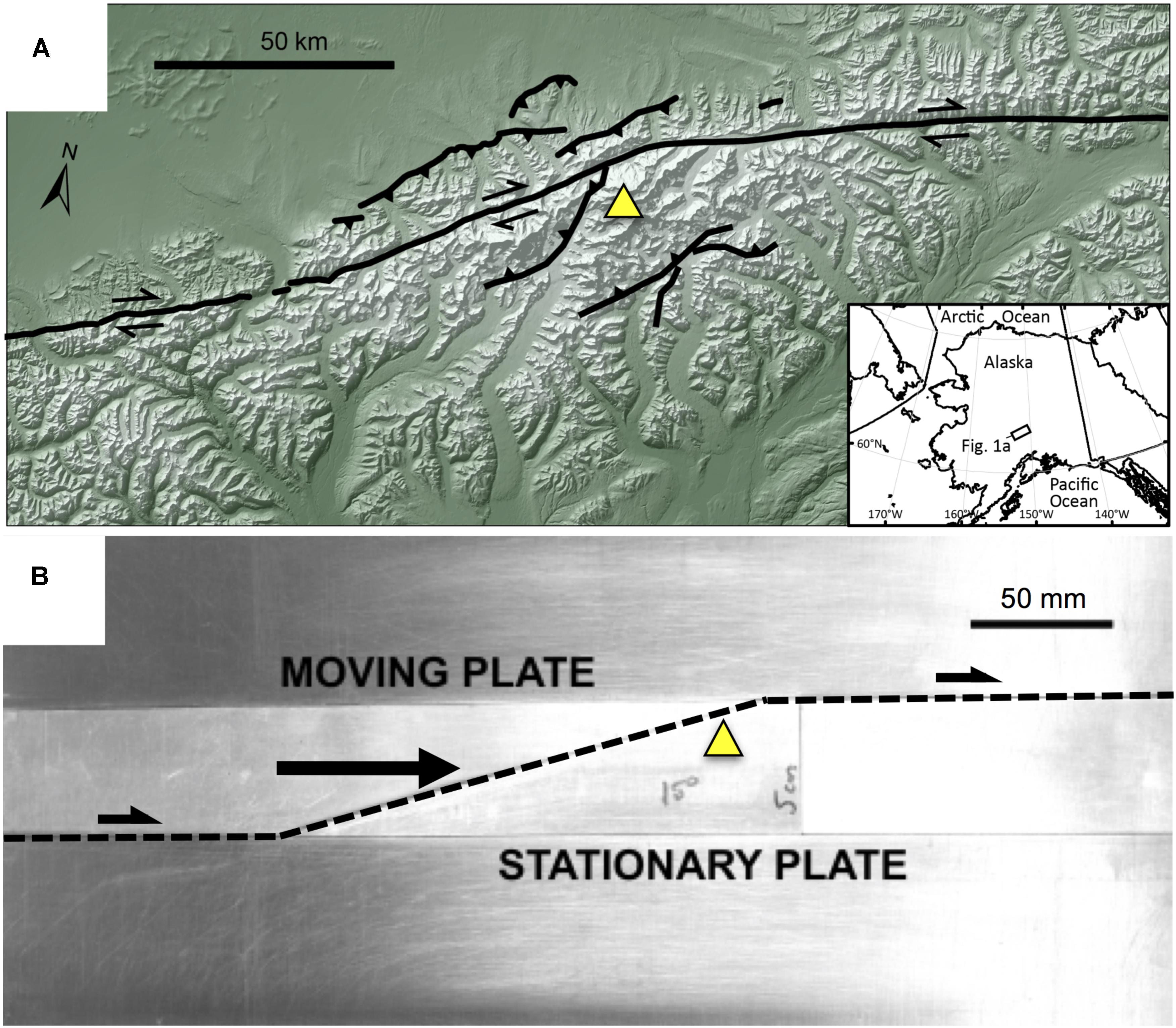
FIGURE 1. (A) Digital elevation model of the Mt. McKinley restraining bend with Denali peak (triangle) and fault trace indicated. Fault traces simplified from Haeussler (2008), Koehler et al. (2012), and Burkett et al. (2016). Shaded-relief base derived from the 2 arcsecond National Elevation Dataset DEM (https://nationalmap.gov/). (B) Basal plate restraining bend configuration (15°, 5 cm stepover) for experimental setup.

Deformation along the modern Alaska Range associated with the Denali fault began in the early Miocene, 16–23 million years ago (e.g., Ridgway et al., 2007; Benowitz et al., 2011). Exhumation and uplift associated with growth of the Alaska Range was spatially variable (Benowitz et al., 2011, 2013; Bemis et al., 2012), with the most prominent feature of the Alaska Range, Denali, initiating rapid exhumation at ∼6 Ma (e.g., Fitzgerald et al., 1995). This exhumation is associated with a major left-step in the Denali fault, forming highly asymmetric and localized topography, within a restraining bend termed the Mount McKinley restraining bend (Fitzgerald et al., 2014; Burkett et al., 2016). Through new quaternary geologic mapping across the eastern portion of the restraining bend, Burkett et al. (2016) identified a number of previously unknown active faults and argued that the locations and sense of slip on these faults place clear limitations on the evolution of the restraining bend system and associated advection of material. However, the limitations of field data and uncertainties of dating deformation make it difficult to directly relate the structural evolution to exhumation recorded in exposed units. Scaled physical experiments can strengthen our field interpretations by demonstrating the relationships between fault system evolution and exhumation path and timings.

Carefully scaled physical experiments reproduce crustal deformational processes that take place on time and length scales, which are otherwise impossible to directly witness (e.g., Cooke et al., 2016; Reber et al., 2017). Scaled experiments of restraining bends have provided critical insights into the development of these structures (Richard et al., 1995; McClay and Bonora, 2001; Dooley and Schreurs, 2012; Cooke et al., 2013; Hatem et al., 2015). These experiments use a variety of techniques to capture the deformation within restraining bends, such as tracking the horizontal displacement of surface marks between photos (McClay and Bonora, 2001; Dooley and Schreurs, 2012; Cooke et al., 2013) and laser scans for uplift (Dooley and Schreurs, 2012; Cooke et al., 2013). Hatem et al. (2015) used successive images taken from a single consumer level DSLR camera and processed using the digital image correlation (DIC) tool, particle image velocimetry (PIV) software, to provide high-resolution displacement perpendicular to the camera view angle. PIV identifies unique patterns of pixels in successive digital images and calculates the displacement vector between them using a Eulerian reference frame. Previous analog modeling studies have successfully demonstrated how PIV can document two-dimensional deformation in a variety of analog materials (e.g., Adam et al., 2005; Cruz et al., 2008; Hatem et al., 2017; Rosenau et al., 2017; Ritter et al., 2018). Similar to PIV, particle tracking velocimetry (PTV) uses image correlation to compare successive images and calculate displacements. Unlike PIV though, PTV identifies individual surface markers between images and calculates a Lagrangian flow path for each marker.

Determining the three-dimensional migration of material in the Mount McKinley restraining bend requires linking horizontal advection with vertical displacement of material in the experiment. Two-dimensional DIC methods (PIV and PTV) use a single camera perspective and fail to provide information about movements in the z plane. For this paper, we will consider that the camera is set up above the experiment to observe horizontal displacement with PIV and PTV but misses uplift deformation. As of 2018, currently available three-dimensional PIV systems (e.g., LaVision DaVis StrainMaster^®) require proprietary software and highly specialized cameras costing upward of $50,000. Here, we present a cost-effective methodology to determine the full three-dimensional advection path of materials using two standard DSLR cameras and a combination of PIV, PTV, and stereovision techniques. The stereovision methodology uses computer vision methods to document vertical deformation within the laboratory. The combination of stereovision with traditional two-dimensional DIC to quantify the vertical and horizontal displacements can be accomplished for less than a tenth of the cost of alternative three-dimensional PIV systems and requires only consumer level cameras, a current Matlab^® license, and several Matlab^® Toolboxes. By adding a second camera to the system, we are able to use stereovision to measure displacement in the z plane (toward and away from the camera) to record the complete three-dimensional deformation. Here, we show how to combine PIV, PTV, and stereovision tools to produce three-dimensional migration paths and show how these methods contribute to our understanding of material movement through the Mount McKinley restraining bend, both horizontal advection along and uplift within the restraining bend.

Materials and Methods

In this section, we first describe how we set up an experiment to simulate deformation within the Mount McKinley restraining bend and then outline the stereovision and PTV methods and approach used to document movement of material through the experimental restraining bend.

Simulating the Mount McKinley Restraining Bend in the Laboratory

To simulate deformation of the restraining bend along the Denali fault, we use bi-viscous wet kaolin. With ∼70% by weight water, the low cohesive strength of wet kaolin provides a material that can scale crustal deformation within a table-top experiment (e.g., Cooke et al., 2016). This material has been used for investigations into the evolution of normal faulting (e.g., Adam et al., 2005; Leever et al., 2011; Hatem et al., 2015), thrust faulting (Cooke and van der Elst, 2012), and strike-slip faulting (e.g., Henza et al., 2010). By adjusting the water content, the clay is prepared to a shear strength of ∼100 Pa, to ensure proper length scaling, and set onto restraining bend configured base plates following Hatem et al. (2015). Using an electrified probe to minimize drag, we precut a 15° restraining bend across a 4 cm thick layer of wet kaolin to approximate the Denali fault’s geometry (Figure 2). Computer controlled stepper motors drive displacement of one of the basal plates to produce a discontinuity at the base of the fault.

FIGURE 2

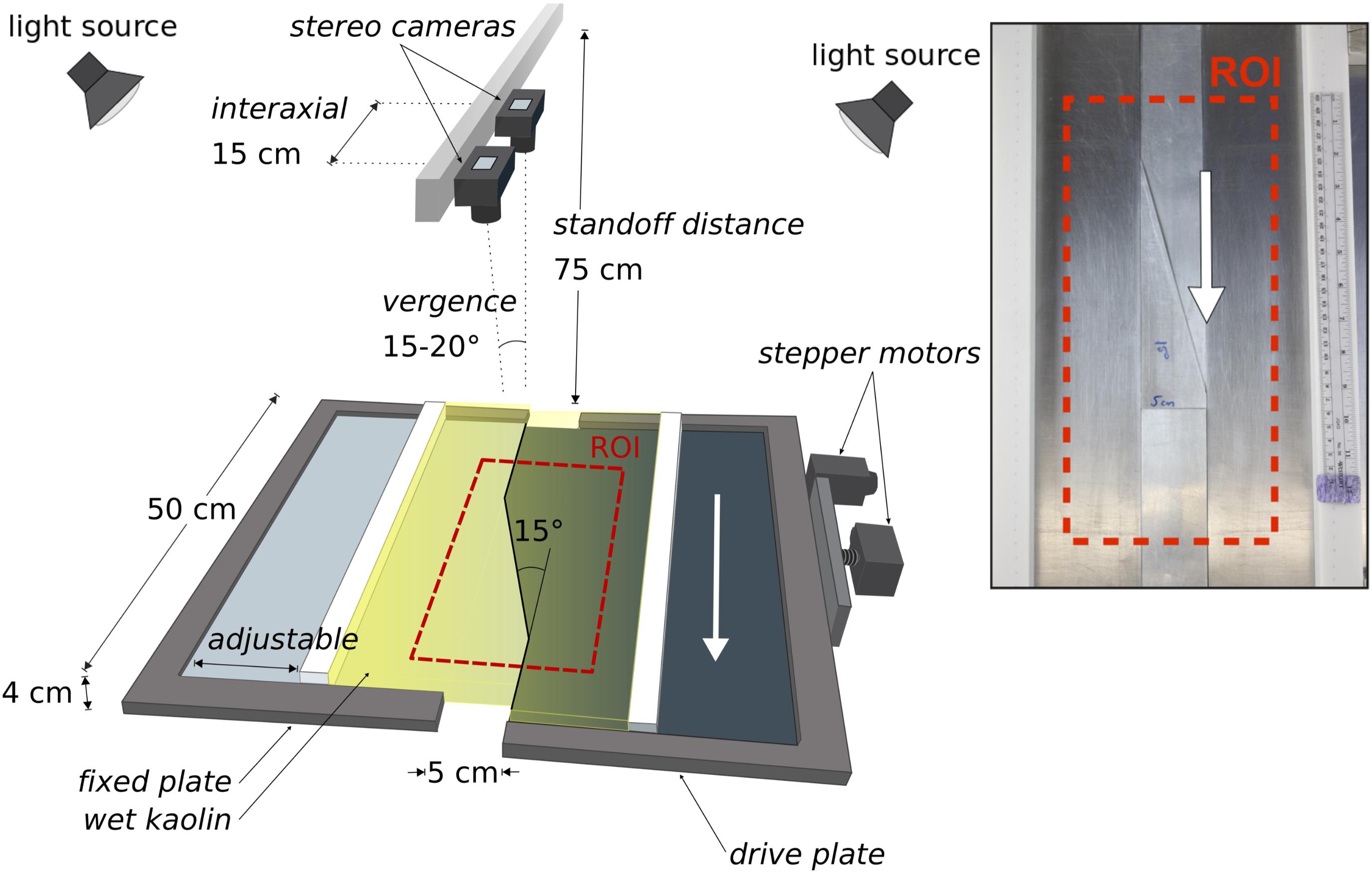
FIGURE 2. Setup for the experiment that simulates the Mount McKinley restraining bend. (Inset) Basal steel plates fitted with triangular aluminum inserts (15°, 5 cm wide) drive the overlying wet kaolin clay with right-lateral displacement. The triangular restraining segment is attached to the fixed plate and overlaps the driving plate. The red dashed box indicates the fixed region of interest (ROI) for image analysis.

To scale the table top experiment to the crustal features of the Mount McKinley restraining bend, two factors need to be considered: the scale of the restraining bend and the slip rate on the fault. Past experiments with wet kaolin have scaled the length of the experiments to the crust (e.g., Henza et al., 2010; Hatem et al., 2015, 2017; Bonanno et al., 2017), but have not considered how the rate of viscous stress relaxation in the kaolin scales to stress relaxation in the crust. Viscous flow within the bi-viscous wet kaolin can simulate the stress dissipation by various pervasive deformation mechanisms in the crust (e.g., cleavage development, microcracking, etc.) if the strain rates are appropriately scaled. The limited range of motor speed necessitated some compromise in scaling of both fault slip rate and length. To scale the fault slip rate, we consider the time-dependent rheology of both the crust and the wet kaolin. The crust has a viscous stress relaxation time of ∼2 Mya (e.g., Bonanno et al., 2017), whereas the relaxation time for kaolin is ∼15 min (e.g., Cooke et al., 2013; Hatem et al., 2015, 2017). Within 15 min of experiment time, we want the fault to accommodate the equivalent of slip that accumulates along Denali fault over 2 Ma. The average slip rate outside of the Mount McKinley restraining bend is approximately 6.5 mm/year (e.g., Turcotte and Schubert, 2014) producing ∼14 km of slip over a period of 2 Mya. Using the fastest motor speed of 2.5 mm/min, the experiment can produce 37.5 mm of slip within 15 min. Setting the 15 min of lab deformation equivalent to 14 km of slip over 2 Ma of crustal deformation gives a length scaling of 1 cm of clay to 3.8 km of crust. This length scaling is consistent with the calculated range of scaling for similar strength wet kaolin (Henza et al., 2010). The restraining segment along the Denali fault measures between 65–70 km in length and forms an ∼18° bend along its trace (Cooke and van der Elst, 2012). Using the length scaling (1 cm: 3.8 km), we simulate this restraining bend in our device using a 15° bend with 19 cm restraining segment (Figure 1). The 4 cm thickness of the clay layer means that we simulate only the upper 15 km of the crust.

We use computer software to take photographs at regular intervals throughout the experiment. The most effective time interval for DIC (PIV and PTV) and stereovision depends on resolution of horizontal and vertical motions and differs for the different techniques as discussed below. Generally, PIV has the finest displacement resolution and all photos are taken at the optimal interval for this analysis. For PTV and stereovision, we use subsets of the recorded photos that represent the optimal time intervals for these analyses. For DIC, photos should be undistorted prior to analysis. Both camera and lens type contribute to distortion. We perform the undistortion in batch form using Adobe Photoshop. This software can also be used to convert color images to black and white, which reduces file size and expedites image analysis. Table 1 lists the material, hardware and software used for the experimental analysis of this study.

TABLE 1

TABLE 1. List of materials used to conduct physical experiments and the necessary software for processing the data.

Stereovision

Stereovision combines two images taken from two different angles to generate depth information for a shared field of view. Before creating a three-dimensional view, the cameras and images must be calibrated. By calibrating the cameras with a grid of known spacing and distance from the imaging sensors, the elevation of common points in the images are correlated to the change in pixel location (pixel disparity). Using the Matlab^® Image Processing Toolbox and the Stereo Camera Calibrator App in the Computer Vision System Toolbox,^TM the user can extract depth information from the two-dimensional image pairs of the experiment.

Acquiring accurate depth information from a photo pair requires several considerations, including:

(1) the desired working distance (standoff distance),

(2) the angle and spacing of the cameras (vergence and interaxial distance),

(3) the focal length of the lenses,

(4) the amount of available light,

(5) the desired spatial and temporal resolution.

Since the total uplift in the restraining bend claybox experiments ranges from a few millimeters to 2 cm, we require very fine vertical resolution in order to capture the incremental elevation change at stages throughout the experiment. Increasing resolution requires either increasing focal length, reducing the working distance, or using a higher resolution sensor. In order to maintain a cost-effective system, we use the standard 18.0 Megapixel complementary metal oxide semiconductor (CMOS) sensors from a pair of consumer grade DSLR cameras at 75 cm standoff distance (Figure 2). Therefore, to improve resolution we are limited to increasing the focal length and/or decreasing the standoff distance—actions that also reduce the field of view. The field of view must remain large enough, however, to capture the faulted region of interest within the experiment. This balance between field of view and resolution must be adjusted on a case-by-case basis.

A pair of Canon Rebel T3i^® cameras with standard 18–55 mm kit lenses provide sub-millimeter vertical resolution. The cameras have an interaxial spacing of 15 cm (Figure 2) combined with a standoff distance of 75 cm and lens focal length of 35 mm, shutter speed (1/60), ISO 100. For this application, we found using a converging field of view (vergence) between 15°–20° as the best compromise between the size of the field of view and the accuracy of depth measurements (Figure 2). Brightly lit surfaces with minimal glare serve best for stereo analysis. We use two identical lamps (four 1600 Lumen LED bulbs) with soft-box light diffusers to provide illumination and turn off the laboratory’s overhead fluorescent to reduce glare on the horizontal surface of the clay (Figure 2).

Calibration and Validation

Extracting depth information from stereo pair images requires careful calibration. Each camera and camera lens have unique intrinsic and extrinsic parameters that vary with focal length and camera position. Before undistorting the images and extracting accurate depth information, we must first measure each of these parameters. Furthermore, we must perform a new calibration any time that the position or focus of a camera is changed. Consequently, once calibrations are completed, we take great care not to disturb the cameras throughout the duration of the experiment.

To determine the calibration parameters, we capture a minimum of 20 stereo pair images of a calibration grid (black and white checkerboard, 23.1 mm squares) that is set at varying orientations and load the photos into the Stereo Camera Calibrator App in the Computer Vision Toolbox^TM of Matlab^®. The software identifies the corners of the grid in each image and determines its three-dimensional orientation. Accurate corner detection requires sharp printing and a consistently flat grid surface. Depending on laboratory humidity, paper may distort between calibration sessions reducing calibration accuracy. We recommend printing on either an overhead transparency sheet or Mylar paper to maintain a dimensionally consistent grid. To calculate depth, the images are rectified or row aligned, reducing the problem to two dimensions (position along x-axis and pixel disparity). The pixel disparity is a measure of change in pixel location between common points from each camera view. The Computer Vision Toolbox^TM combines the known calibration grid spacing to convert the pixel disparity maps to real-world distance maps. We repeat the calibration, removing, and replacing stereo pairs, until the overall mean reproduction error reported by the Stereo Camera Calibrator App is less than 1 pixel. The reproduction error is a measure of the average pixel distance between a detected point projected in the image and the same point reprojected after processing (MathWorks^®, 2018). The Stereo Camera Calibrator application produces a unique stereo parameters object that contains both intrinsic and extrinsic parameters and can be exported and combined with new pairs of photos to generate suites of digital elevation models of the clay surface for each experiment using functions within the Computer Vision Toolbox^TM of Matlab^®.

We import the parameters calculated from the calibration procedure into the built-in Matlab^® Computer Vision Toolbox^TM function rectifyStereoImage. Using the functions stereoAnaglyph, and disparity provided in the Computer Vision Toolbox^TM, we, respectively, create and then convert the pixel disparity map generated from the pairs of photos taken throughout the experiment, into real-world distances from the camera. By subtracting the known distance of the camera from the working surface (working distance), we can then convert these data into a digital elevation model. We validate the calibrated system by comparing the stereovision created digital elevation model of a simple wedge with direct measurements of the wedge’s slope and height. The angled surface provides a continuous gradient of heights to ensure accuracy over a greater depth of field in addition to providing a direct comparison to a known real-world surface. Vertical errors vary within ±1 mm between calibration sessions.

The optimal interval of photos to use in stereovision analysis depends on the vertical errors from the validation and the rate of elevation change of the experiment. With stereovision elevation errors of ±1 mm, photos taken in quick succession of a slowly uplifting feature will not resolve the small (<1 mm) changes in elevation between each photo. Within the restraining bend experiment, we see ∼15 mm of total uplift over 48 min. The rate of uplift rate increases in the latter half of the experiment, so the change in elevation between successive pairs of photos exceeds the vertical error of the analysis.

Calculating Incremental Uplift Pattern

The incremental uplift between pairs of photos is calculated by subtracting the topography of the earlier pair from the later pair. However, as the stepper motors drive deformation, the horizontal position of structures in the clay change relative to the fixed field of view of the cameras. As a result, calculating incremental uplift from the difference in elevation between individual time steps can produce artificial uplift due to shifting locations of structures between steps (Figure 3a). We correct for this shift by adjusting the horizontal position of points in the DEM using results from the PIV analysis. PIV analysis with the PIVlab Matlab^® application (Matmon et al., 2006; Mériaux et al., 2009; Haeussler et al., 2017) uses just one photo from each of the stereopairs to produce a grid of incremental horizontal displacements between each step. The grid from the PIV is often at lower resolution than the DEM from stereovision necessitating re-gridding of one or the other datasets. Once the datasets have matching horizontal grids, the incremental horizontal displacements from the PIV can be subtracted from the point locations of the later DEM to shift the later structures to their earlier positions. The resulting difference in elevation between the later and earlier DEM provides the incremental uplift pattern due to active faulting (Figure 3b). This approach compensates for the horizontal drift between frames and improves the accuracy of the incremental uplift maps. Around the middle of the experiment, the accuracy of the stereovision elevation is compounded by the relatively low uplift rates (compared to late in the experiment) to reduce the quality of the incremental uplift pattern (Figure 3c).

FIGURE 3

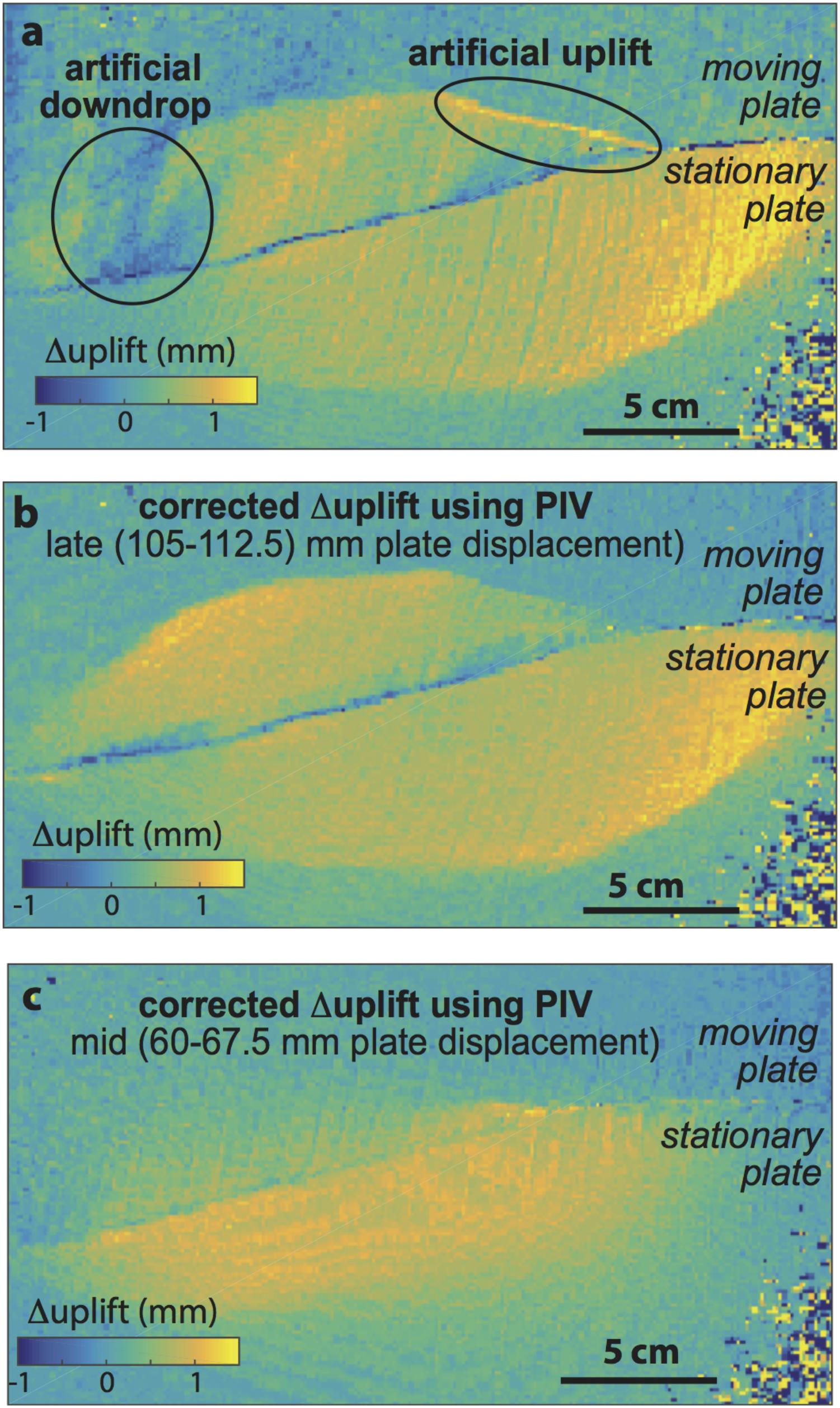
FIGURE 3. Example incremental uplift maps showing the change in surface elevation over a 7.5 mm increment of applied plate displacement late in the experiment. The lower resolution of the incremental uplift maps compared to the cumulative uplift map reflects the downgrading of the DEM to the resolution of the PIV in order to adjust the horizontal position of migrating structures. (a) The differences between elevation at 112.5 and 110 m of plate displacement without PIV correction. The highlighted regions contain artificial down-drop and uplift due to lateral movement of the clay morphology on the moving plate. (b) The change in elevation for the same interval of plate displacement as A but using the PIV data to correct for the lateral movement. The artificial elevation changes are removed and the resulting change in morphology corresponds to fault activity during this period. (c) Incremental uplift for a 7.5 mm stage near the middle of the experiment.

Particle Tracking Velocimetry Methodology

Particle tracking velocimetry is a DIC technique that detects groups of pixels belonging to non-deforming objects/particles and tracks their two-dimensional displacements in successive images. Using a Lagrangian frame of reference, PTV calculates a flow path for each marker, tracking the migration of material throughout an experiment (Figure 4). The technique has been used in fluid mechanics research for several decades (e.g., Maas et al., 1993; Ohmi and Li, 2000). Within geoscience applications, PTV has been used to measure water flow and discharge within water sheds (Muste et al., 2008; Patalano et al., 2017). For this study, we use the free Matlab^® plug-in, PTVlab, developed by Patalano & Wernher and based on PIVlab Version 1.2 2009 by W. Thielicke. Both PTVlab and PIVlab rely on the Image Processing Toolbox within Matlab^®.

FIGURE 4

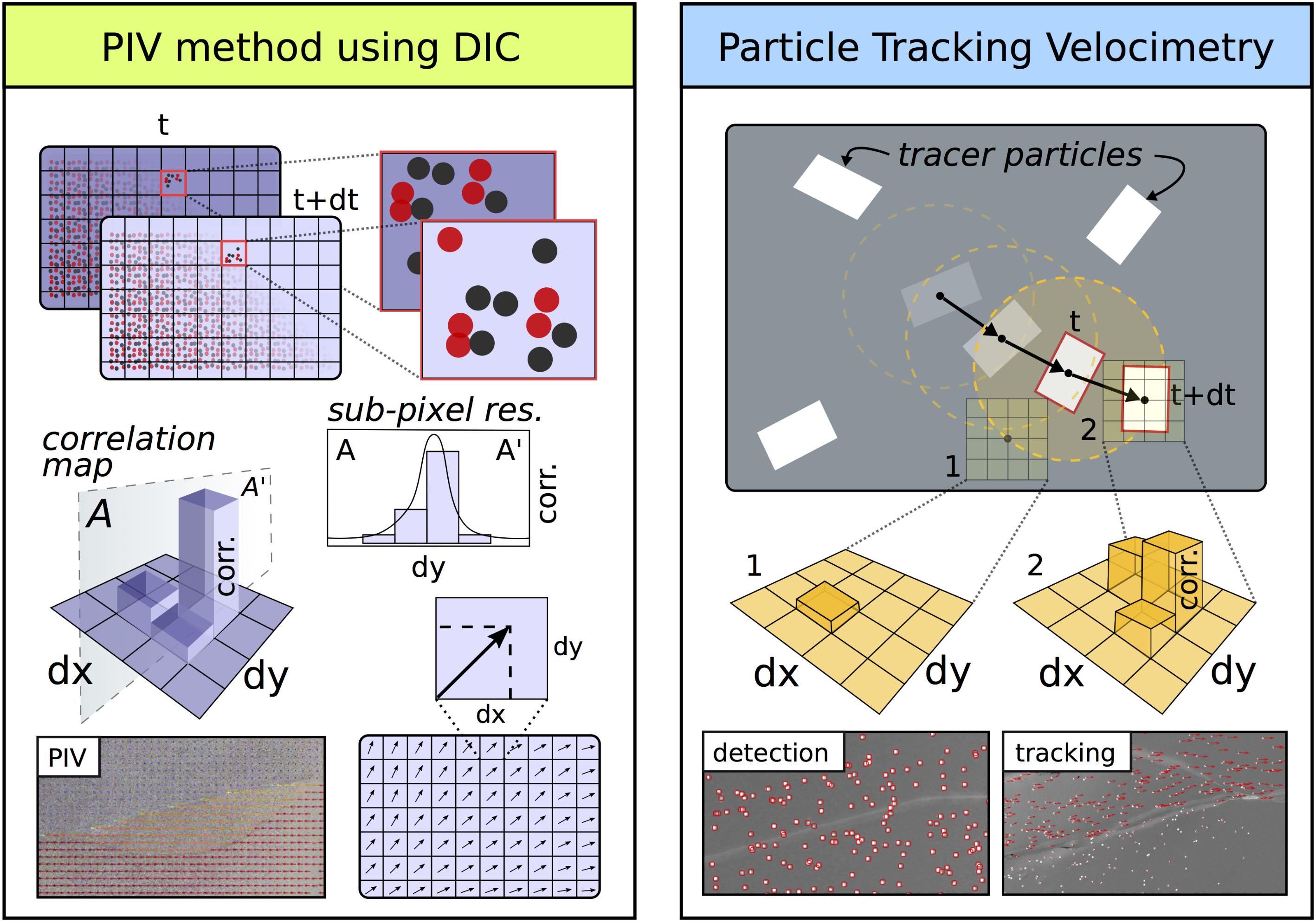
FIGURE 4. Particle image velocimetry (PIV) method employs digital image correlation (DIC) to measure the change in displacement within each gridded cell for a sequence of images (left panel). The grid remains fixed within a Eularian reference frame with cell size predetermined based on the expected displacement increment and desired spatial resolution. Within each gridded cell, small high-contrast surface markers form a unique pattern that is used to identify each cell’s vector of displacement between two sequential frames. A correlation map identifies the grid-locations (dx, dy) with the strongest match from the previous frame. Fitting the correlation map with a Gaussian curve allows for sub-pixel spatial resolution. PTV, however, employs a non-fixed Lagrangian reference frame to track the displacement and velocity of individual particles. The tracer particles are detected based on size and color contrast with the background image and then given unique identifiers (bottom right). Between frames, the area around each particle is searched using a grid to identify the location with the strongest matching pattern (top right). The radius of the grid search is likewise dependent on the displacement increment and the desired spatial resolution.

The most notable difference between the two-dimensional PTV and PIV techniques is how the images are processed (Figure 4). In PIV, pixels within a grid of windows from successive image pairs are cross-correlated to calculate change in displacement between the two photos. The change in displacement from each window contributes to the gridded displacement field. This method provides very precise and complete coverage of the incremental displacement fields. In contrast, PTV identifies individual markers, gives them unique labels, and tracks their migration throughout each subsequent image.

Since PTV relies on being able to detect and correlate unique particles in each image of the experiment, acquiring accurate PTV results requires many of the same setup considerations as stereovision and PIV techniques, such as high-resolution photos and bright non-glare producing lighting. Unlike in stereovision, however, a single camera can be used to extract the two-dimensional flow paths of the particles. We used the images from one of the two stereovision cameras for PTV analysis collected at 1 min intervals throughout the experiment.

Setting Up Particle Detection

When selecting markers to use for PTV, high color contrast and image resolution should be considered in order ensure that the Gaussian Mask detection algorithm can properly identify the markers at the desired resolution. Since our clay surface is off-white, we chose high contrast black foil pieces (craft glitter) with ∼1 mm² area. Because we recorded PTV simultaneously with stereovision, we required the marker’s profile on the surface to be undetectable by stereovision—making the thin foil an ideal marker for our application. PTVlab’s detection algorithms are designed to detect white particles, so we invert the color in all of the images before loading them into MATLAB^® (e.g., Figure 5A). Additionally, the correlation threshold, sigma (number of pixels), and the intensity thresholds for the detection algorithm must be adjusted per application to differentiate the white markers from the background surface/noise. For our photos, we used a fixed a minimum correlation of 0.4 and neighbor similarity of 25% to detect the craft glitter in the inverted photographs.

FIGURE 5

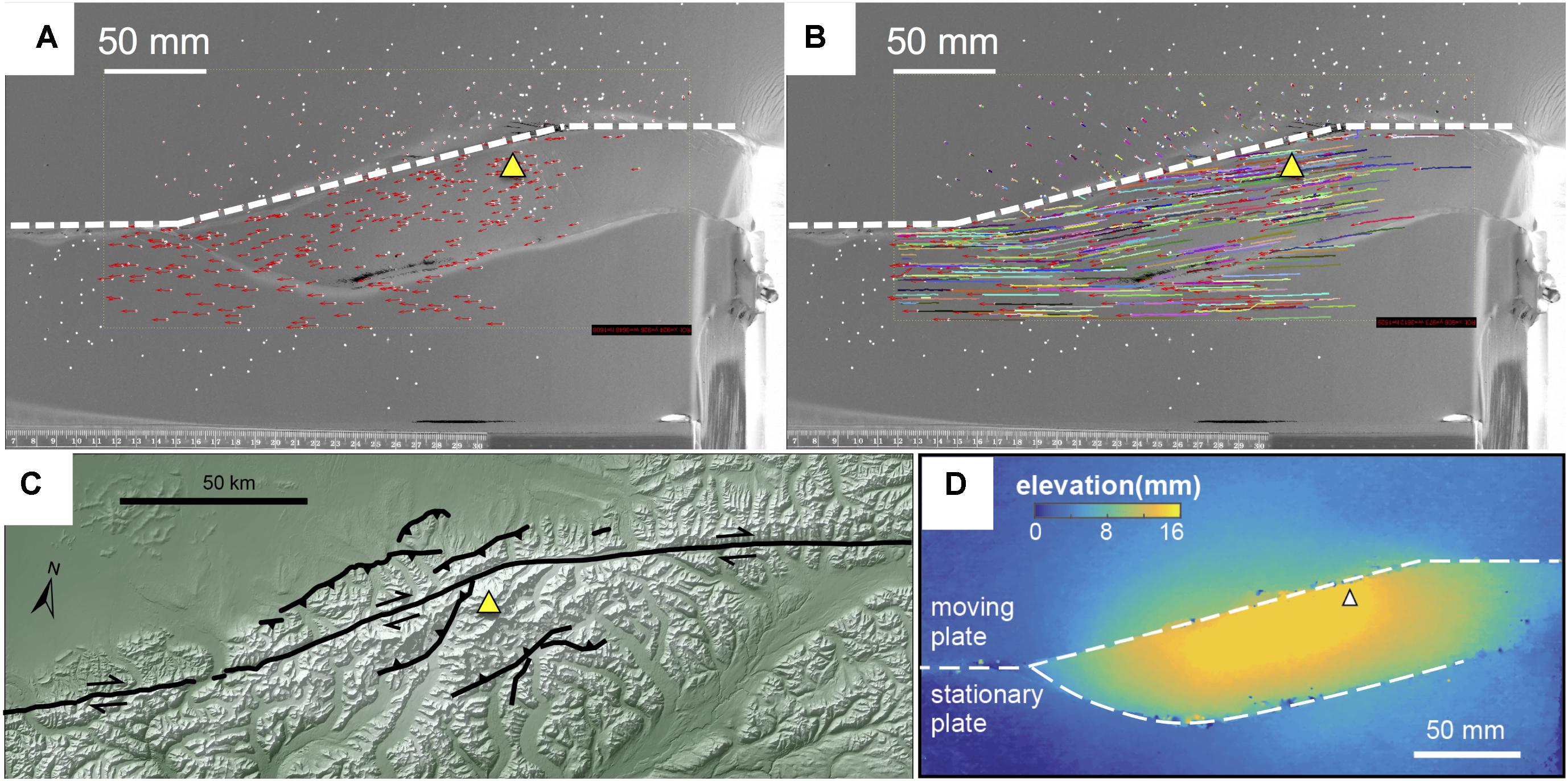
FIGURE 5. Particle tracking velocimetry (PTV) showing (A) incremental and (B) cumulative advective transport around a physical model designed to simulate the Mount McKinley restraining bend along the Denali fault zone. (C) Digital elevation model of the Denali fault with Denali peak (triangle) and fault trace indicated. (D) Cumulative uplift map revealed by stereovision.

Fine resolution of results requires small interrogation windows for the cross-correlation. Consequently, the displacement increment between photos cannot be larger than the window size since the software searches within the window for the pixel cluster of the object. For fast experiments, this requires frequent photos. We use an interrogation window size of 10 sq-pixels (0.77 mm² for our photos) to record the small incremental displacements (0.25 mm/image) in our experiments. The markers used for PTV tracking must be small enough to be detected within the interrogation window. We found that for this interrogation window size, markers with an upper size limit of ∼1 mm² yielded the most accurate marker detection. Since the particle tracking algorithms are computationally expensive, greater number of particles can quickly overwhelm your CPU. For our experiment, we continuously tracked several hundred particles randomly distributed across the surface of the experiment.

The results of the PTV analysis are extracted as a MATLAB^® cell array. The particle path information can be extracted from PTV results using the Langranpath function included with PTVlab. This function sorts information from the cell array by the identification numbers that PTVlab assigns to each detected particle and the Langranpath function stores the track information in a new n by 1 structure, where n is the number of particles detected. Each unit of the nx1 structure has the x- and y-positions of the particle through time that can be plotted as a streamline (Figure 5B). Not all the particles distributed on the kaolin surface were successfully tracked throughout the experiment. Figures 6b,c display the paths from a subset of the 235 particles that were tracked from the start to the end of the experiment. The colors of the streamlines in Figures 6b,c indicate the uplift of the particle as it advects along the fault. To assign the uplift information to each particle we co-located the PTV and stereovision datasets. Once co-located, the PTV dataset provides x- and y-coordinates of the particle throughout the experiment that can be queried from the uplift dataset in order to find the three-dimensional particle path (Figures 6b,c). We performed the PTV and PIV analyses over several hours on an Inspiron 660 standard desktop PC built in 2013. This computer is currently out of date; newer computers with faster processors could perform the analysis more quickly and with greater number of particles.

FIGURE 6

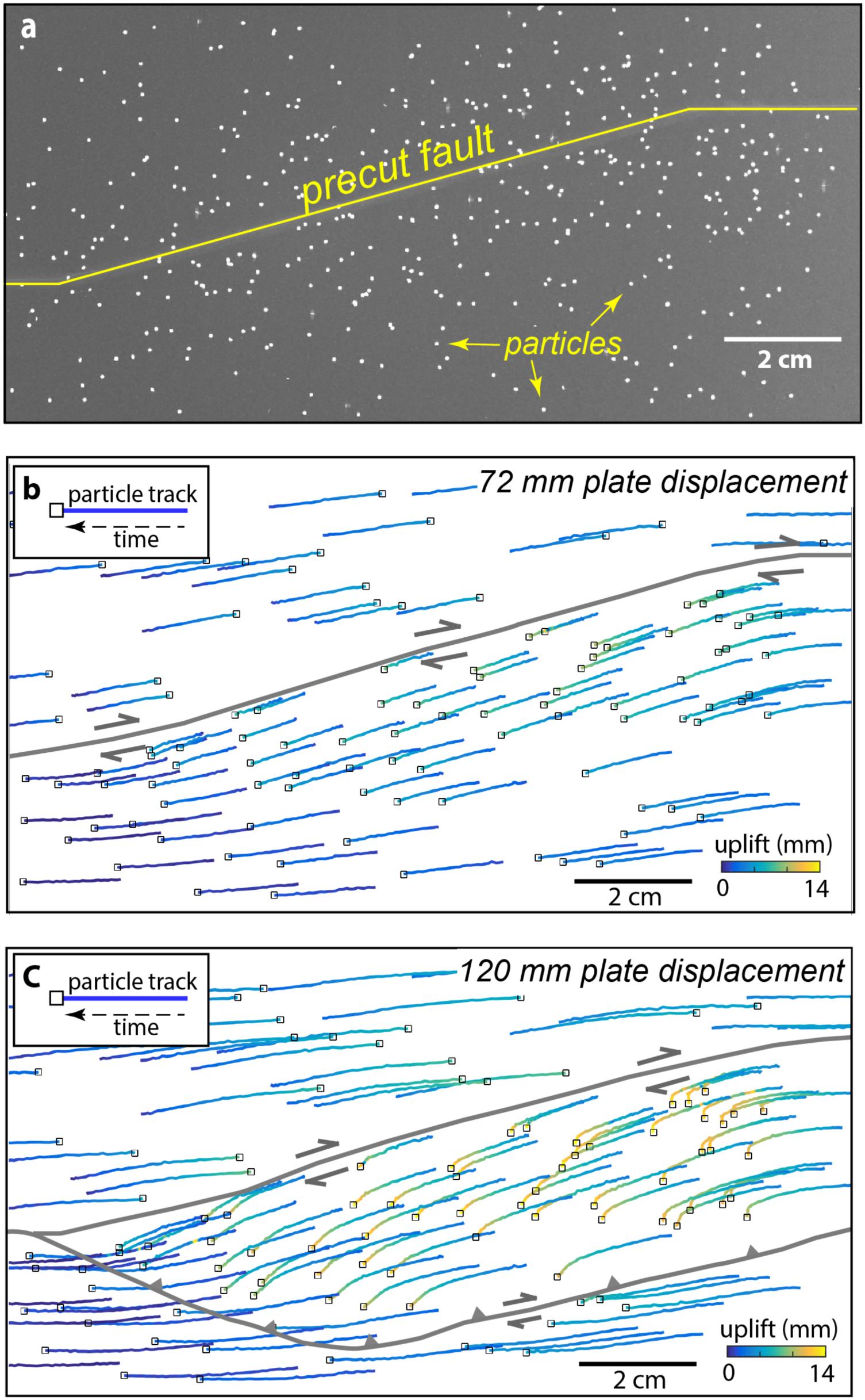
FIGURE 6. (a) Inverted photo used for PTV analysis with black markers on off-white kaolin at the start of the experiment. Flow paths generated from particle tracking velocimetry (PTV) show material migrating through a 15° restraining bend claybox experiment in a fault-fixed reference frame. Color indicates uplift history of each particle. (b) Early in the experiment displacement is predominantly parallel to the fault with modest uplift. (c) With growth of the new oblique-slip fault, the particles change trajectory and uplift.

Performing both PIV and PTV on the same experimental photos can be tricky. The fine resolution of the incremental displacement field from PIV requires many more particles that can be reasonably tracked with the PTV analysis. For our investigation of the Mount McKinley restraining bend with homogeneously textured kaolin, we used two different experiments that were each optimized for the different DIC approaches. One experiment had thousands of sand grains sprinkled on the surface of the clay to provide pixel texture for the PIV analysis (Figures 3, 5D) and another experiment had ∼250 pieces of glitter for the PTV analysis (Figure 6). Photos that contain both thousands of fine particles and hundreds of larger particles could be used for PTV analysis as the fine particles could be filtered out before the analysis. However, using these same photos for PIV may be more problematic. The larger particles will likely create holes in the finer resolution PIV analysis, which would require data conditioning. As long as the markers do not impact the surface topography, uplift data using stereovision tools can be collected from pairs of photos regardless of marker size or spacing.

Results

The cumulative uplift map shows the development of asymmetric high topography around the experimental restraining bend (Figure 5D) that resembles the asymmetric topography of the Mt. McKinley restraining bend (Figure 5C). The highest topography develops above the stationary plate and is associated with the development of a new thrust fault outboard of the initial 15° restraining segment. This morphology is consistent with that recorded in similarly configured restraining bends experiments that use high-precision laser scanners (e.g., Cooke et al., 2013). Hatem et al. (2015) show that the asymmetry arises from the moving basal plate moving over the stationary plate within the restraining bend. This accounts for why restraining bends that have basal plates that move toward one another (at equal displacement rates), and not one over the other, produce symmetric uplift (McClay and Bonora, 2001; Thielicke and Stamhuis, 2014). Comparisons of the final clay surface elevation (Figure 7B) to minimum rock uplift surfaces calculated by thermochronologic data (Figure 7A) and modern topography (Figure 7C) reveal striking first-order similarity in topographic asymmetry across the Denali fault. In both the experiment and the geologic data, the greatest cumulative uplift occurs adjacent to the restraining segment of the fault and decreases with distance from the fault (Figures 7A–C). In contrast, the strike-slip segments of the fault beyond both ends of the restraining segment do not produce a significant uplift signature. The mountainous topography along the Denali fault outside of the restraining bend has elevations that are thousands of meters lower than the topography adjacent to the restraining segment (Figure 7C), and both the regional geology and preliminary thermochronologic data (Burkett et al., 2016) indicate only limited late Cenozoic exhumation. The development of the new oblique-slip fault outboard of the pre-cut restraining bend in the experiment corresponds to Neogene thrust faults mapped to the south of the of the Denali fault, some of which are noted to exhibit oblique-slip (Haeussler, 2008; Figure 7). Similarly, the localized band of uplift and highly oblique particle trajectories on the north side of the restraining segment in the experiment (Figures 5D, 6) is consistent with the occurrence of several active thrust faults that trend sub-parallel to the restraining segment (Burkett et al., 2016; Figures 1A and 7C). While patterns of uplift are remarkably similar, elevation differences between the experiment and geologic constraints (Figures 7D,E) highlight the experiment’s inability to capture erosion, isostatic response, and differential erodibility of units. Erosion factors into the geologic constraints at two primary scales. First, glacial erosion localized across the higher elevations of the restraining bend drives a crustal isostatic response, producing exhumation values that exceed the scaled experimental uplift on the order of 4–5 km (Figure 7D). Second, erosion of broad U-shaped valleys by the major glaciers, particularly along the Denali fault, produce narrow bands where the scaled experimental uplift exceeds the minimum uplift constraints by 2–4 km. Also, the contrast in erodibility between the broadly fractured granitic plutons and the pervasively deformed and fractured Jurassic-Cretaceous sediments of the region (Reed and Nelson, 1980; Haeussler, 2008) likely contributes to the significant topographic relief development illustrated by the two peaks in Figure 7E where the minimum uplift surface exceeds the scaled experimental uplift by up to 1.5 km.

FIGURE 7

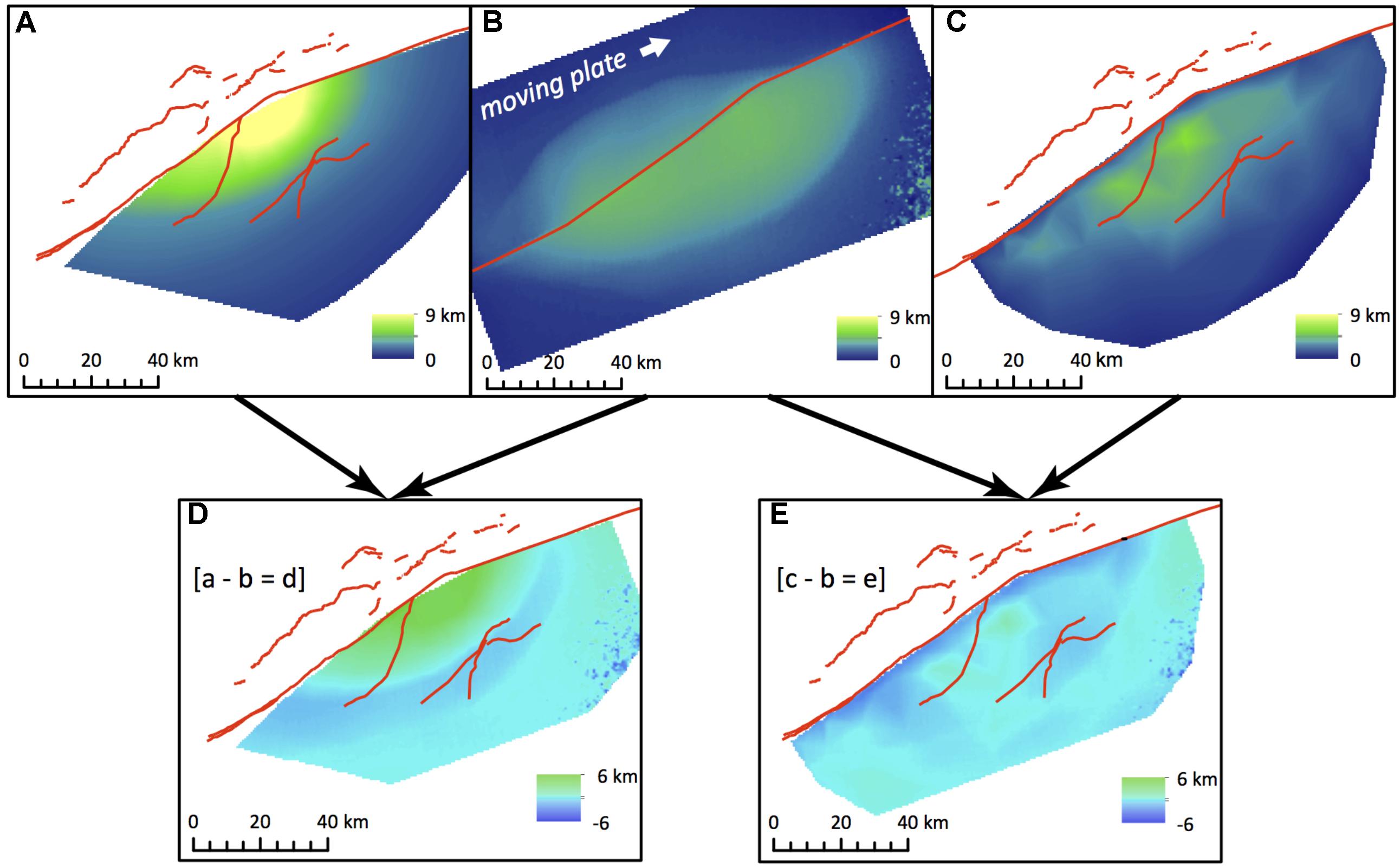
FIGURE 7. Surfaces representing two geologic constraints on uplift in the Mount McKinley restraining bend (A,C) and the surface from the wet kaolin analog experiments (B). Red lines illustrate modern fault traces derived from Reed and Nelson (1980), Haeussler (2008), and Burkett et al. (2016). (A) A rock uplift surface derived from low-temperature thermochronology (Fitzgerald et al., 1995). (B) Equivalent elevation map of the clay experiment, using the scaling relationships of the experiment to convert into the scale of geologic constraints (Fendick, 2016). (C) An approximation of a minimum rock uplift surface derived by extrapolating between modern peak and ridge elevations in the Mount McKinley restraining bend (Fendick, 2016). Surfaces (D) and (E) are difference maps used to compare the cumulative uplift in the experiment (B) to the geologic constraints (A,C). (D) The difference between thermochronology-derived uplift (A) and the experiment (B). (E) The difference between the minimum rock uplift (C) and the experiment (B). Positive values (green) represent areas where the experiment did not produce as much uplift as the geologic constraints and negative values (blue) show where the experiment produced more uplift.

Incremental uplift maps show changes in uplift pattern with thrust fault activity (Figure 3). During the early activity of the outboard faults (60–67.5 mm of basal plate displacement), off-fault deformation increases uplift rate in the hanging wall of the new thrust fault (Figure 3c). At this stage, the greatest uplift rates are adjacent to the precut restraining segment of the fault. Later in the experiment, as the new outboard faults grow and link, the zone of uplift widens to include both hanging walls of the newly created thrust faults (110–112.5 mm basal plate displacement; Figure 3b). The greatest uplift rates are then along the traces of the new faults.

Flow paths from PTV analysis show advection of material through the experimental restraining bend (Figure 6). Within the experiment, one basal plate moves relative to the other so the faults drift with respect to the overhead stationary camera. In Figure 6, we change the reference frame so that the fault remains fixed and markers positioned above the stationary plate appear to move leftward. Prior to the development of the outboard fault, the markers near the fault move parallel to the pre-cut fault segment (Figure 6b). Throughout the experiment markers far from the faults move predominantly in the direction of basal plate movement with modest uplift. With the growth of the new fault, the markers above the stationary plate and in the hanging wall of the oblique-slip fault show an abrupt southward change of particle direction and increase in uplift after ∼75 mm of total plate displacement (Figure 6c). This rapid change in the horizontal trajectory occurs when the uplift pattern suggests growth of the outboard faults.

In this study, we have presented results from two experiments with identical boundary and starting conditions that can be compared to assess repeatability. Aleatory uncertainty due to variable material and experimental conditions naturally occurs within physical experiments so that repeated experiments may give different results (e.g., Schreurs et al., 2016). Both the experiment with sand on the surface of the kaolin (optimal for PIV) and the experiment with glitter distributed on the surface of the clay (optimal for PTV) show development of a new outboard fault that accommodates oblique slip. Both experiments show similar pattern of faulting. One difference between the experiments is the segmented nature of the outboard fault in the PIV optimized experiment (Figure 3) compared to the continuous fault trace in the PTV optimized experiment (Figure 6). This difference is not expected to impact the finding of advection through the restraining bend. Repeated restraining bend experiments with the same device and material used in this experiment show variability of fault slip rates of up to 10% of the motor speed (Hatem et al., 2015; Figure 3b).

Discussion/Conclusion

The stereovision combined with PTV DIC provides a useful approach for tracking advection of several hundred points through the restraining bend. However, the irregular and loose spacing of the PTV particles would not serve well for problems that require high resolution of the displacement or strain fields. For example, mapping active faults and measuring slip rates is better performed with the denser sampling available with PIV DIC.

Other popular techniques exist for extracting 3D topographic data from natural and experimental settings; however, these present challenges for tracking incremental horizontal and vertical displacements through the course of a scaled physical experiment. For example, laser scanners can be used to scan the surface of experiments with comparable resolution. The drawback of laser scanners is that they take several minutes to set up and produce the scan during which the experiment must be stopped. Hatem et al. (2015) show that for time dependent rheology, such as the bi-viscous wet kaolin, stresses within the experiment can dissipate significantly during the time of capturing the laser scan, which impacts the results. Another potential approach is photo-based 3D reconstruction methods (often referred to as structure-from-motion or SfM), which facilitates the creation of a 3D point cloud of a target through the collection of multiple overlapping photographs taken from different viewing angles (e.g., James and Robson, 2012; Westoby et al., 2012; Bemis et al., 2014). The resulting point cloud is effectively the same as those produced through airborne laser swath mapping (ALSM/LIDAR) and lab-based laser scanning tools. Several studies have successfully used these point clouds to measure differential displacements observed in earthquakes and displacements artificially introduced into LIDAR topographic datasets (Nissen et al., 2012, 2014; Scott et al., 2018). However, the iterative-closest-point algorithms employed by these studies rely on a certain degree of topographic complexity to determine unique 3D displacements between the two point clouds. Our experiments exhibit relatively smooth surfaces beyond the localized fault zones; thus, we suspect that iterative-closest-point methods would produce a noisy displacement field at best. Furthermore, this technique requires a windowed/tiled measurement approach (e.g., Nissen et al., 2012), requiring significant processing for a single displacement step. Other algorithms can efficiently calculate differences between point clouds (C2C, M3C2; Lague et al., 2013), but these are unable to account for lateral displacements.

Popular open-source photogrammetry and PIV software MicMac (Galland et al., 2016), TecPIV (Boutelier, 2016), and OpenPIV¹ provide similar functionality to the built-in Matlab^® stereovision application and PIVlab plug-in. Open source software does not depend on access to Matlab^® though some require Python, which is open source. However, for integration between datasets and further analysis in Matlab^®, these programs would create an even more cumbersome workflow. The user-friendly GUI and abundant documentation for both the Matlab^® Stereovision App and PIVlab plug-in were important factors in maintaining a practical, in addition to cost-effective, methodology.

While stereovision in combination with DIC can provide both horizontal and vertical displacements of the experiment, the two datasets are not integrated as they would be with the off-the-shelf three-dimensional PIV systems, such as LaVision DaVis StrainMaster^®. The extra effort to coordinate between the stereovision uplift dataset and the DIC horizontal displacement dataset, however, is offset by the relative cost savings of using Matlab^® based software, available at many institutions. The results of this effort shed insight into the three-dimensional path of material as it advects through the restraining bend.

The calibrated stereovision system reliably produces uplift maps of the clay surface within the experiments with ±1 mm accuracy (∼5% net uplift for a typical experiment). When combined with horizontal displacements, these elevation data describe the three-dimensional deformation within the evolving fault systems, such as advection and uplift of material along restraining bends. In our simulations of the Mt. McKinley restraining bend, we show that the development of outboard thrust faults shifts the trajectory of material advection. The development of the thrust faults also increases the uplift rate of material within the restraining bend, which is revealed from the combination of horizontal and vertical displacements. The uplift/subsidence rate and pattern can be directly calculated by differencing elevation data across sequential time steps. This approach can be used to relate change in fault evolution to changes in uplift rate. Our simulation of the Mount McKinley restraining bend shows that the loci of greatest uplift rate changes during evolution of the fault system from www.openpiv.net/

near the strike-slip fault to adjacent to the new thrust fault traces. Uplift rate maps can also provide the dip slip rate along faults with knowledge of the fault dip, which can be estimated by introducing a trench into the analog material. By combining the horizontal displacement field data with elevation data collected with stereovision techniques, geologists have a new inexpensive tool to quantify the three-dimensional structural evolution of crustal systems in scaled physical experiments.

Data Availability

The raw data supporting the conclusions of this manuscript will be made available by the authors, without undue reservation, to any qualified researcher.

Author Contributions

KT performed the experiments, collected the data, and wrote first draft of the manuscript. MC, JB, and SB contributed conception and design of the study. KT developed the stereovision workflow and algorithm. MC developed the PTV processing algorithm. KT and MC performed the data analysis. MC and SB wrote sections of the manuscript. SB and JB provided geologic background on Denali fault and motivation for study. AF compiled thermochronology and modern day topographic uplift constraints for the Mount McKinley restraining bend. All authors contributed to manuscript revision, read, and approved the submitted version.

Funding

This work was supported partially by the National Science Foundation under Grant No. EAR 1250461 to SB, Grant No. EAR 1550133 to MC, and Grant No. EAR 1249885 to JB.

Conflict of Interest Statement

The authors declare that the research was conducted in the absence of any commercial or financial relationships that could be construed as a potential conflict of interest.

Acknowledgments

The authors thank Tim Dooley, Cara Burberry, and a third reviewer for helpful reviews that helped strengthen the paper.

References

Adam, J., Urai, J. L., Wieneke, B., Oncken, O., Pfeiffer, K., Kukowski, N., et al. (2005). Shear localisation and strain distribution during tectonic faulting—new insights from granular-flow experiments and high-resolution optical image correlation techniques. J. Struct. Geol. 27, 283–301. doi: 10.1016/j.jsg.2004.08.008

CrossRef Full Text | Google Scholar

Bemis, S. P., Carver, G. A., and Koehler, R. D. (2012). The Quaternary thrust system of the northern Alaska Range. Geosphere 8, 196–205. doi: 10.1130/ges00695.1

CrossRef Full Text | Google Scholar

Bemis, S. P., Micklethwaite, S., Turner, D., James, M. R., Akciz, S., Thiele, S. T., et al. (2014). Ground-based and UAV-Based photogrammetry: a multi-scale, high-resolution mapping tool for structural geology and paleoseismology. J. Struct. Geol. 69, 163–178. doi: 10.1016/j.jsg.2014.10.007

CrossRef Full Text | Google Scholar

Benowitz, J. A., Layer, P. W., Armstrong, P., Perry, S. E., Haeussler, P. J., Fitzgerald, P. G., et al. (2011). Spatial variations in focused exhumation along a continental-scale strike-slip fault: the Denali fault of the eastern Alaska Range. Geosphere 7, 455–467. doi: 10.1130/ges00589.1

CrossRef Full Text | Google Scholar

Benowitz, J. A., Layer, P. W., and Vanlaningham, S. (2013). Persistent Long-term (c. 24 Ma) Exhumation in the Eastern Alaska Range constrained by stacked thermochronology. Geological Society. London: Special Publications 378, SP378. 312.

Google Scholar

Bonanno, E., Bonini, L., Basili, R., Toscani, G., and Seno, S. (2017). How do horizontal, frictional discontinuities affect reverse fault-propagation folding? J. Struct. Geol. 102, 147–167. doi: 10.1016/j.jsg.2017.08.001

CrossRef Full Text | Google Scholar

Boutelier, D. (2016). TecPIV—A MATLAB-based application for PIV-analysis of experimental tectonics. Comput. Geosci. 89, 186–199. doi: 10.1016/j.cageo.2016.02.002

CrossRef Full Text | Google Scholar

Burkett, C. A., Bemis, S. P., and Benowitz, J. A. (2016). Along-fault migration of the mount mckinley restraining bend of the denali fault defined by late quaternary fault patterns and seismicity, denali national park & preserve, Alaska. Tectonophysics 693, 489–506. doi: 10.1016/j.tecto.2016.05.009

CrossRef Full Text | Google Scholar

Cooke, M. L., Reber, J. E., and Haq, S. (2016). Physical experiments of tectonic deformation and processes: building a strong community. GSA Today 26:36. doi: 10.1130/gsatg303gw.1

CrossRef Full Text | Google Scholar

Cooke, M. L., Schottenfeld, M. T., and Buchanan, S. W. (2013). Evolution of fault efficiency at restraining bends within wet kaolin analog experiments. J. Struct. Geol. 51, 180–192. doi: 10.1016/j.jsg.2013.01.010

CrossRef Full Text | Google Scholar

Cooke, M. L., and van der Elst, N. J. (2012). Rheologic testing of wet kaolin reveals frictional and bi-viscous behavior typical of crustal materials. Geophys. Res. Lett. 39:L01308. doi: 10.1029/2011gl050186

CrossRef Full Text | Google Scholar

Cruz, L., Teyssier, C., Perg, L., Take, A., and Fayon, A. (2008). Deformation, exhumation, and topography of experimental doubly-vergent orogenic wedges subjected to asymmetric erosion. J. Struct. Geol. 30, 98–115. doi: 10.1016/j.jsg.2007.10.003

CrossRef Full Text | Google Scholar

Cunningham, W. D., and Mann, P. (2007). Tectonics of Strike-Slip Restraining and Releasing Bends: Fig. 1. Geological Society, Vol. 290. London: Special Publications, 1–12. doi: 10.1144/sp290.1

CrossRef Full Text | Google Scholar

Dooley, T. P., and Schreurs, G. (2012). Analogue modelling of intraplate strike-slip tectonics: a review and new experimental results. Tectonophysics 57, 1–71. doi: 10.1016/j.tecto.2012.05.030

CrossRef Full Text | Google Scholar

Elliott, A., Oskin, M., Liu-zeng, J., and Shao, Y.-X. (2018). Persistent rupture terminations at a restraining bend from slip rates on the eastern Altyn Tagh fault. Tectonophysics 733, 57–72. doi: 10.1016/j.tecto.2018.01.004

CrossRef Full Text | Google Scholar

Fendick, A. M. (2016). Denali in a Box: Analog Experiments Modeled After a Natural Setting Provide Insight on Gentle Restraining Bend Deformation. MS thesis, University of Kentucky, Kentucky.

Google Scholar

Fitzgerald, P. G., Roeske, S. M., Benowitz, J. A., Riccio, S. J., Perry, S. E., and Armstrong, P. A. (2014). Alternating asymmetric topography of the Alaska range along the strike-slip Denali fault: strain partitioning and lithospheric control across a terrane suture zone. Tectonics 2013:TC003432. doi: 10.1002/2013TC003432

CrossRef Full Text | Google Scholar

Fitzgerald, P. G., Sorkhabi, R. B., Redfield, T. F., and Stump, E. (1995). Uplift and denudation of the central Alaska Range: a case study in the use of apatite fission track thermochronology to determine absolute uplift parameters. J. Geophys. Res. 100, 20175–20191. doi: 10.1029/95JB02150

CrossRef Full Text | Google Scholar

Galland, O., Bertelsen, H. S., Guldstrand, F., Girod, L., Johannessen, R. F., Bjugger, F., et al. (2016). Application of open-source photogrammetric software MicMac for monitoring surface deformation in laboratory models. J. Geophys. Res. 121, 2852–2872. doi: 10.1002/2015JB012564

CrossRef Full Text | Google Scholar

Haeussler, P. J. (2008). An overview of the neotectonics of interior Alaska: far-field deformation from the Yakutat microplate collision. Active Tecton. Seismic Potent. Alaska 179:20080101.

Google Scholar

Haeussler, P. J., Matmon, A., Schwartz, D. P., and Seitz, G. G. (2017). Neotectonics of interior Alaska and the late Quaternary slip rate along the Denali fault system. Geosphere 13, 1445–1463. doi: 10.1130/GES01447.1

CrossRef Full Text | Google Scholar

Hatem, A. E., Cooke, M. L., and Madden, E. H. (2015). Evolving efficiency of restraining bends within wet kaolin analog experiments. J. Geophys. Res. 120, 1975–1992. doi: 10.1002/2014jb011735

CrossRef Full Text | Google Scholar

Hatem, A. E., Cooke, M. L., and Toeneboehn, K. (2017). Strain localization and evolving kinematic efficiency of initiating strike-slip faults within wet kaolin experiments. J. Struct. Geol. 101, 96–108. doi: 10.1016/j.jsg.2017.06.011

CrossRef Full Text | Google Scholar

Henza, A. A., Withjack, M. O., and Schlische, R. W. (2010). Normal-fault development during two phases of non-coaxial extension: an experimental study. J. Struct. Geol. 32, 1656–1667. doi: 10.1016/j.jsg.2009.07.007

CrossRef Full Text | Google Scholar

James, M., and Robson, S. (2012). Straightforward reconstruction of 3D surfaces and topography with a camera: accuracy and geoscience application. J. Geophys. Res. 117:F03017. doi: 10.1029/2011JF002289

CrossRef Full Text | Google Scholar

Koehler, R. D., Farrel, R.-E., Burns, P. A. C., and Combellick, R. A. (2012). Quaternary Faults and Folds in Alaska: A Digital Database. Alaska Division of Geological & Geophysical Surveys Miscellaneous Publication, 141, 31. doi: 10.14509/23944

CrossRef Full Text | Google Scholar

Lague, D., Brodu, N., and Leroux, J. (2013). Accurate 3D comparison of complex topography with terrestrial laser scanner: application to the Rangitikei canyon (NZ). ISPRS J. Photogramm. Remote Sens. 82, 10–26. doi: 10.1016/j.isprsjprs.2013.04.009

CrossRef Full Text | Google Scholar

Lease, R. O., Haeussler, P. J., and O’Sullivan, P. (2016). Changing exhumation patterns during Cenozoic growth and glaciation of the Alaska Range: insight from detrital geo- and thermo-chronology. Tectonics 2015:TC004067. doi: 10.1002/2015TC004067

CrossRef Full Text | Google Scholar

Leever, K. A., Gabrielsen, R. H., Sokoutis, D., and Willingshofer, E. (2011). The effect of convergence angle on the kinematic evolution of strain partitioning in transpressional brittle wedges: insight from analog modeling and high-resolution digital image analysis. Tectonics 30:F03017. doi: 10.1029/2010tc002823

CrossRef Full Text | Google Scholar

Maas, H., Gruen, A., and Papantoniou, D. (1993). Particle tracking velocimetry in three-dimensional flows. Exp. Fluids 15, 133–146. doi: 10.1007/BF00190953

CrossRef Full Text | Google Scholar

Matmon, A., Schwartz, D., Haeussler, P., Finkel, R., Lienkaemper, J., Stenner, H. D., et al. (2006). Denali fault slip rates and Holocene–late Pleistocene kinematics of central Alaska. Geology 34, 645–648. doi: 10.1130/G22361.1

CrossRef Full Text | Google Scholar

McClay, K., and Bonora, M. (2001). Analog models of restraining stepovers in strike-slip fault systems. AAPG Bull. 85, 233–260.

Google Scholar

McGill, S. F., Owen, L. A., Weldon, R. J., and Kendrick, K. J. (2013). Latest Pleistocene and Holocene slip rate for the San Bernardino strand of the San Andreas fault, Plunge Creek, Southern California: implications for strain partitioning within the southern San Andreas fault system for the last 35 k.y. Geol. Soc. Am. Bull. 125, 48–72. doi: 10.1130/b30647.1

CrossRef Full Text | Google Scholar

Mériaux, A. S., Sieh, K., Finkel, R. C., Rubin, C. M., Taylor, M. H., Meltzner, A. J., et al. (2009). Kinematic behavior of southern Alaska constrained by westward decreasing postglacial slip rates on the Denali fault, Alaska. J. Geophys. Res. 114:B03404. doi: 10.1029/2007JB005053

CrossRef Full Text | Google Scholar

Muste, M., Fujita, I., and Hauet, A. (2008). Large-scale particle image velocimetry for measurements in riverine environments. Water Resour. Res. 44:W00D19. doi: 10.1029/2008WR006950

CrossRef Full Text | Google Scholar

Nissen, E., Krishnan, A. K., Arrowsmith, J. R., and Saripalli, S. (2012). Three-dimensional surface displacements and rotations from differencing pre-and post-earthquake LiDAR point clouds. Geophys. Res. Lett. 39:16301. doi: 10.1029/2012GL052460

CrossRef Full Text | Google Scholar

Nissen, E., Maruyama, T., Arrowsmith, J. R., Elliott, J. R., Krishnan, A. K., Oskin, M. E., et al. (2014). Coseismic fault zone deformation revealed with differential lidar: examples from Japanese Mw 7 intraplate earthquakes. Earth Planet. Sci. Lett. 405, 244–256. doi: 10.1016/j.epsl.2014.08.031

CrossRef Full Text | Google Scholar

Ohmi, K., and Li, H.-Y. (2000). Particle-tracking velocimetry with new algorithms. Measur. Sci. Technol. 11:603. doi: 10.1088/0957-0233/11/6/303

CrossRef Full Text | Google Scholar

Patalano, A., García, C. M., and Rodríguez, A. (2017). Rectification of image velocity results (RIVeR): a simple and user-friendly toolbox for large scale water surface particle image velocimetry (PIV) and particle tracking velocimetry (PTV). Comput. Geosci. 109, 323–330. doi: 10.1016/J.CAGEO.2017.07.009

CrossRef Full Text | Google Scholar

Reber, J. E., Dooley, T. P., and Logan, E. (2017). Analog modeling recreates millions of years in a few hours. EOS 98, doi: 10.1029/2017EO085753

CrossRef Full Text | Google Scholar

Reed, B., and Nelson, S. (1980). Geologic Map of the Talkeetna Quadrangle, Alaska. USGS Misc. Investigations Series, Map I-1174. Reston, VA: US Geological Survey.

Google Scholar

Richard, P., Naylor, M., and Koopman, A. (1995). Experimental models of strike-slip tectonics. Petrol. Geosci. 1, 71–80.

Google Scholar

Ridgway, K. D., Thoms, E. E., Layer, P. W., Lesh, M. E., White, J. M., and Smith, S. V. (2007). “Neogene transpressional foreland basin development on the north side of the central Alaska Range, Usibelli Group and Nenana Gravel, Tanana basin,” in Tectonic Growth of a Collisional Continental Margin: Crustal Evolution of Southern Alaska Geological Society of America Special Paper, eds K. D. Ridgway, J. M. Trop, J. M. G. Glen, and J. M. O’Neill (Boulder, CO: Geological Society of America), 507–547.

Google Scholar

Ritter, M. C., Santimano, T., Rosenau, M., Leever, K., and Oncken, O. (2018). Sandbox rheometry: co-evolution of stress and strain in Riedel– and Critical Wedge–experiments. Tectonophysics 722, 400–409. doi: 10.1016/j.tecto.2017.11.018

CrossRef Full Text | Google Scholar

Rosenau, M., Corbi, F., and Dominguez, S. (2017). Analogue earthquakes and seismic cycles: experimental modelling across timescales. Solid Earth 8, 597–635. doi: 10.5194/se-8-597-2017

CrossRef Full Text | Google Scholar

Schreurs, G., Buiter, S. J. H., Boutelier, J., Burberry, C., Callot, J.-P., Cavozzi, C., et al. (2016). Benchmarking analogue models of brittle thrust wedges. J. Struct. Geol. 92, 116–139. doi: 10.1016/j.jsg.2016.03.005

CrossRef Full Text | Google Scholar

Scott, C. P., Arrowsmith, J. R., Nissen, E., Lajoie, L., Maruyama, T., and Chiba, T. (2018). The M 7 2016 Kumamoto, Japan, Earthquake: 3-D Deformation Along the fault and within the damage zone constrained from differential lidar topography. J. Geophys. Res. 123, 6138–6155. doi: 10.1029/2018JB015581

CrossRef Full Text | Google Scholar

Thielicke, W., and Stamhuis, E. (2014). PIVLab—Time-resolved digital particle image velocimetry tool for MATLAB. PIV ver. 1.32”.).

Google Scholar

Turcotte, D., and Schubert, G. (2014). Geodynamics. Cambridge: Cambridge University Press. doi: 10.1017/CBO9780511843877

CrossRef Full Text | Google Scholar

Westoby, M., Brasington, J., Glasser, N., Hambrey, M., and Reynolds, J. (2012). ‘Structure-from-Motion’photogrammetry: a low-cost, effective tool for geoscience applications. Geomorphology 179, 300–314. doi: 10.1016/j.geomorph.2012.08.021

CrossRef Full Text | Google Scholar