 Heidi M. Dierssen
- Department of Marine Sciences, University of Connecticut, Groton, CT, United States
Breaking waves are highly reflective features on the sea surface that change the spectral properties of the ocean surface in both magnitude and spectral shape. Here, hyperspectral reflectance measurements of whitecaps from 400 to 2,500 nm were taken in Long Island Sound, USA of natural and manufactured breaking waves to explore new methods to estimate whitecap contributions to ocean color imagery. Whitecap reflectance was on average ~40% in visible wavelengths and decreased significantly into the near infrared and shortwave infrared following published trends. The spectral shape was well-characterized by a third order polynomial function of liquid water absorption that can be incorporated into coupled ocean-atmospheric models and spectral optimization routines. Localized troughs in whitecap reflectance correspond to peaks in liquid water absorption and depths of the troughs are correlated to the amount and intensity of the breaking waves. Specifically, baseline-corrected band depths at 980 and 1,200 nm explained 77 and 90% of the whitecap-enhanced reflectance on a logarithmic scale, respectively. Including these wavebands into future ocean color sensors could potentially provide new tools to estimate whitecap contributions to reflectance more accurately than with wind speed. An effective whitecap factor was defined as the optical enhancements within a pixel due to whitecaps and foam independent of spatial scale. A simple mixed-pixel model of whitecap and background reflectance explained as much of the variability in measured reflectance as more complex models incorporating semi-transparent layers of foam. Using an example atmosphere, enhanced radiance from whitecaps was detectable at the top of the atmosphere and a multiple regression of at-sensor radiance at 880, 1,038, 1,250, and 1,615 nm explained 99% of the variability in whitecap factor. A proposed model of whitecap-free reflectance includes contributions from water-leaving radiance, glint, and diffuse reflected skylight. The epsilon ratio at 753 and 869 nm commonly used for aerosol model selection is nearly invariant with whitecap factor compared to the ratio at shortwave infrared bands. While more validation data is needed, this research suggests several promising avenues to retrieve estimates of the whitecap reflectance and to use ocean color to further elucidate the physics of wave breaking and gas exchange.
Introduction
Breaking wind-waves or whitecaps are highly reflective features on the sea surface that change the spectral properties of the ocean surface in both magnitude and spectral shape. Whitecaps are weakly absorbing, highly light-scattering media (Kokhanovsky, 2004). At wind speeds of around 3 m s−1 and higher, waves can break and entrain air in the water which subsequently breaks up into bubbles which rise to the surface (Thorpe, 1982; Monahan and O'Muircheartaigh, 1986). The presence of breaking waves or whitecaps serves to significantly enhance the reflectance of the sea surface measured by aircraft or satellites. Since the seminal work by Gordon and Wang (1994), atmospheric correction approaches for ocean color imagery have included models to account for elevated reflectance of whitecaps. This study builds off of the research from the last few decades to provide new insights into hyperspectral approaches for estimating whitecap contributions for satellites of varying spatial resolutions.
The amount of whitecaps on the sea surface is commonly characterized as a fractional coverage of the sea with actively breaking waves. The fractional whitecap coverage is relatively small across the global ocean (<1%), but can be up to 10% in very active seas (Zhao and Toba, 2001; Brumer et al., 2017). This fractional component includes Stage A whitecap representing the actively breaking wave or bright white portion of the wave (Monahan, 1993). Elevated reflectance also occurs due to the residual plume of foam and subsurface bubbles that is referred to as a Stage B whitecap. Differentiating between these two stages is challenging and it is unclear as to how much of the Stage B plume is included in different methods of estimating whitecap fraction. With image analysis methods, the foam portion of Stage B is generally included in the estimate of whitecap fraction, but elevated reflectance from the submerged bubble plume is not often visible in photography (Brumer et al., 2017). A recent study taken in high wind conditions of the Southern Ocean suggests fractional whitecap coverage retrievals from a radiometer were consistently higher than estimates from high-resolution digital photographs due to the enhanced sensitivity of the radiometer and the ability to detect more of the decaying bubble plume area (Randolph et al., 2017).
The use of a whitecap fraction is appropriate for sensors with a 1-km pixel, which is the footprint of most ocean color missions like the proposed hyperspectral mission PACE. However, higher spatial resolution satellites have smaller pixels ranging from 30 m down to 1 m that can resolve individual whitecap features. For example, the proposed hyperspectral missions Enmap and HyspIRI aim to have 30-m pixel resolution (Guanter et al., 2015; Lee et al., 2015). Hence, the fraction of whitecaps within a pixel can be much higher than the average fractional whitecap coverage and can vary from 0 to 1 within a given scene. For example, a pan-sharpened Landsat-8 image (15-m pixels) off the coast of Normandy where winds were 12.5 m s−1 illustrates how ocean swell and the contribution of breaking waves can vary on a pixel-by-pixel basis (Figure 1A). The imagery also highlights how the impact of a ship wake, observed as the larger “white” feature centered in the image, can also impact the observed ocean color in high resolution imagery (Vanhellemont and Ruddick, 2014).
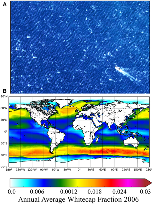
Figure 1. (A) Pseudo-true color image from a 15-m pan sharpened Landsat-8 OLI image from the coast of Normandy with winds estimated at 12.5 m s−1 illustrating whitecap features and a boat wake. (B) Estimate of the average whitecap fraction for 2006 calculated from a parameterization of wind speed and satellite-derived whitecap fraction from microwave brightness temperature. Modified from Albert et al. (2016) with permission from M. Anguelova.
Some of the first measurements of whitecap reflectance were made in the 1980's (Whitlock et al., 1982; Koepke, 1984). While most optical studies dealing with whitecaps and bubbles focus on the visible and near infrared (NIR) wavelengths, limited studies suggest that whitecaps can reflect significantly in the short wave infrared (SWIR) and would interfere with atmospheric correction routines that use SWIR bands (e.g., 1,240 and 1,640 nm) (Whitlock et al., 1982; Frouin et al., 1996; Wright et al., 2012). The reflectance of whitecaps has been modeled using parameterizations of the absorption coefficient of water (Whitlock et al., 1982; Kokhanovsky, 2004). However, as discussed further in this contribution, there were errors in the Whitlock et al. (1982) study, including the water absorption values used in visible wavelengths and the reflectance standard, that make these values inaccurate.
Although technically not a constituent of the atmosphere, corrections for whitecaps, foam, and bubbles are included in the current atmospheric correction routines. Whitecap reflectance is often modeled using an empirical cubic relationship to wind speed and an approximate reflectance value for an individual whitecap (Gordon and Wang, 1994; Ahn et al., 2012). However, such models are overly simplistic and presume that whitecap coverage at an individual daily pixel can be estimated as a simple function of wind speed throughout the world ocean. As shown in many different studies (Anguelova and Webster, 2006; Brumer et al., 2017), instantaneous whitecap coverage can vary by several orders of magnitude at the same wind speed. The fraction of whitecaps can be influenced by the fetch and duration and the wind, water temperature, air temperature and stability of the lower atmosphere defined by the air/water temperature differential, salinity, current shear, and long wave interaction, wave age, and the presence of surfactants such as organic films (reviewed in Scanlon and Ward, 2016). “At different locations in the world ocean, various environmental and meteorological factors act in concert but with different strengths and form a composite effect that either enhances or suppresses the effect of wind alone” (Anguelova and Webster, 2006). Hence, any wind speed parameterization of whitecaps is meant to be climatological rather than instantaneous.
Whitecaps on the sea surface are relevant to air-sea gas exchange, generation of sea spray aerosols and the climate cycle (Blanchard, 1985; Asher and Wanninkhof, 1998; Monahan, 2008). They are especially critical in retrieving accurate ocean color in regions like the Southern Ocean which are characterized by persistent high winds and breaking waves (Figure 1B). Here, new measurements are presented of natural and manufactured whitecaps and foam from the ultraviolet through the shortwave infrared. These data are used to address whether whitecaps can be well-approximated in shape and magnitude by an average whitecap reflectance, what parameterizations can be used to model mixed pixels of varying fractions of whitecaps, and whether more accurate algorithms can be developed to approximate whitecap reflectance for hyperspectral remote sensing applications based on the measured spectrum itself rather than ancillary wind speed.
Methods
The experiments were conducted in Long Island Sound in surface waters near the University of Connecticut Avery Point campus, U.S.A. Sampling included the region known as the Race which spans 5.6 km between Fishers Island and Little Gull Island and serves as the main entrance into Long Island Sound (41°14′36.6″N 72°2′49.2″W). This region is known for a large rip line and large waves due to the depth range from 15 to 75 m coupled with the massive water exchange in and out of Long Island Sound. The water color in this region is peaked in green wavelengths and there are higher amounts of suspended material causing higher backscattered light compared to many other regions of the world ocean (Aurin et al., 2010; Aurin and Dierssen, 2012). However, the waters are not considered turbid (total suspended matter <2 g m−3) and water-leaving reflectance is negligible in NIR and SWIR wavelengths.
Data Collection
Whitecap reflectance was measured using a PANalytical Boulder ASD FieldSpec 4 spectroradiometer with a wavelength range from 350 to 2,500 nm interpolated to a 1 nm resolution under ambient sunlight during clear sky conditions. The sensor was equipped with an 8.5° fore-optic and was optimized for the light field with dark current. The sensor was pointed to a 99% white Spectralon plaque held horizontally to the sea surface at a distance of ~2 cm from the plaque. The plaque was held in a relative azimuth orientation toward the sun to avoid user shading on the measurement. The plaque measurement provided an estimate of downwelling irradiance during the experiment and was taken periodically to normalize the measurement as described further below. After the measurement was taken over Spectralon, the sensor was extended over the target at ~0.5–1.5 m above the sea surface depending on the size of the swell and motion of the boat at an azimuth angle of ~145° from the sun to minimize sun glint. This translates to a field of view covering a 7.5–22-cm diameter circle on the sea surface.
For the natural breaking waves, measurements were made from the side of the R/V Lowell Weicker on 19 January 2016 pointing with a heading into the wind in order to maintain position with the wave field. On this day, wind speed varied from 10 to 12 m s−1 measured at 3 m height at the Eastern Sound Buoy in Long Island Sound (41° 15.48′N, 72° 04.00′W) and significant wave heights estimated to be 1.5–2 m using measurements from the Central Sound Buoy (lisicos.uconn.edu). The background reflectance followed standard NASA protocols where 5-replicates were taken of a sequence of measurements from a 12% spectralon reference panel, water, and sky while maintaining a 45° zenith angle of the sensor. The sensor was positioned at an azimuth angle of ~145° from the sun to minimize sun glint. Whitecap measurements were taken in a time-series mode at 8 ms over a 20-min interval with the radiometer pointing down at a nadir angle at the sea surface for roughly 75,000 samples. Measurements were taken of the 99% spectralon reference panel at the beginning and end of sampling and after every whitecap event in an azimuthal angle facing the sun with the sensor at a nadir angle to the plaque. The time series of measurements taken over rolling breakers were considered to be spectral mixtures of whitecap, foam and undisturbed water. Four different breaking events were measured with varying intensities and contributions of breaking waves.
Measurements were also taken over manufactured breaking waves and foam from various sources including boat wakes and an outflow pipe. During these experiments, the field of view of the sensors was focused on the breaking feature and these measurements are considered to be spectral endmembers of breaking waves/foam without undisturbed water. Forward motion of the 23-m long R/V Connecticut produced a boat wake with a large breaking wave on the side of the ship on 29 June 2017 16:01–16:15 UTC at Race Point Long Island Sound (41° 14.62′N, 72° 02.52′W) with clear skies and a 20° solar zenith angle. In addition, measurements were taken of the boat wake and multiple layers of foam produced by circular motion of a small Carolina Skiff on 25 June 2015. Measurements were also taken of layers of foam produced on the sea surface by an outflow pipe from the high-flow pressurized seawater distribution system at the Rankin Seawater Laboratory, University of Connecticut 27 January 2015.
Data Analysis
Lambertian-equivalent reflectance of the sea surface was calculated as ratio of the measurement obtained of a breaking wave and measurement of the lambertian Spectralon plaque. Normalization was conducted using a recent calibration of the white plaque which varied from 97% in ultraviolet, 99% in visible, and 93% reflective in SWIR wavelengths out to 2,500 nm. No corrections were conducted for reflection of glint or skylight from the sea surface when estimating the reflectance from background water or water enhanced by foam and whitecaps. From a satellite perspective, the removal of sun/sky glint is a separate step from removing whitecap reflectance. Hence, the methods developed here included the sun/sky glint in the background reflectance in order to differentiate the contribution from the whitecap signal from the remaining signal.
Reflectance from breaking waves, foam, and bubbles is treated with different methods in the literature and these different methods are considered in the results section. Because whitecaps are so bright, the signal is commonly thought to dwarf the contributions from water-leaving radiance and reflected skylight or glint and is treated as a “white” patch on the sea surface. For atmospheric correction approaches, the estimated whitecap reflectance is generally considered invariant of the water-leaving signal, sky conditions, and wind speed (Gordon and Wang, 1994). Whitecaps, and particularly bubble plumes, can also be treated as an augmentation above a background reflectance (Moore et al., 2000). The total reflectance (Rt) is considered to be the background water-leaving reflectance (Rb) plus some additional amount due to whitecaps (Raug), such that:
A recent study defined an “augmented reflectance ratio” as the fractional augmentation of a whitecap above a background reflectance (Xu et al., 2015). This definition is not used in this manuscript because it is felt that an augmentation ratio does not properly reflect the physics of the system. A more nuanced approach is to treat whitecaps as a two-layered system where a semi-transparent layer of foam and bubbles overlays a background water reflectance (Frouin et al., 1996), as described further in the results. Radiative transfer modeling based on the theoretical work of Kokhanovsky (2004) and Zege et al. (2006) is presented in the Results. Radiative modeling of whitecaps bridges the measured reflectance to the optical properties of foam.
Whitecap measurements were compared to the absorption coefficient of seawater, aw. The aw (m−1) used in this analysis were calculated for standard ranges of salinity (30–34 ppt) and temperature (0–20°C) encountered in the world ocean using the Water Optical Properties Processor (Rottgers et al., 2011). Differences in aw with temperature and salinity are insignificant to the results presented here out to 2,500 nm, but water properties of 20°C 34 ppt are used for analyses.
Propagation of Sea Spectral Reflectance to the Top of the Atmosphere
Sea surface reflectance is converted to radiance and propagated through the atmosphere to estimate the radiance due to mixed pixels of whitecaps and background at the satellite. First, the reflectance is converted from water-leaving reflectance (Rw = Eu(0+)/Ed(0+)) to an estimate of the upwelling radiance leaving the sea surface in the nadir direction, Lw (note that this definition includes mixed pixels of radiance from foam and bubbles, as well as water-leaving radiance and sea surface reflected diffuse and direct irradiance). This conversion is conducted assuming the sea surface reflectance is lambertian and the downwelling irradiance reaching the sea surface can be approximated by the solar constant, Fo, adjusted by the cosine of the solar zenith angle (θs), the transmission of diffuse irradiance between the sun and earth, tds, and the mean distance between the Sun and Earth, fs, such that for each wavelength:
Finally, this estimate of radiance at the sea surface is attenuated by the intervening atmosphere according to the diffuse transmission factor in the direction of the satellite, tdv. For purposes of this investigation, an experimental atmosphere was used to investigate whether the water impacted by different amounts of foam and whitecap could be detected with an intervening atmosphere containing water vapor and other constituents that could obscure the signal. Hence, experimental values of at-sensor radiance due to Rayleigh scattering (Lr) and aerosols (La) were added to the spectra to create a typical top of the atmosphere radiance spectrum (LTOA). An atmosphere typical to the MOBY buoy (157°11′36″W, 20°49′07″N) was used with a solar zenith angle of 42°, humidity of 72.8%, water vapor of 1.737 g cm−2, and pressure of 1,015.19 mb. No sun glint contribution is considered at TOA because the direct and diffuse reflected skylight was included in the field measurements of water reflectance and propagated through the atmosphere with Lw. This approach neglects any atmospheric effects that may occur due to enhanced reflectance of the sea surface from whitecaps and aerosol-molecular coupling.
The observed epsilon, εobs, is used to assess spectral dependence of aerosols from the TOA radiance and is estimated here for water surfaces with different levels of foam. The observed aerosol reflectance for a given wavelength (λ) was estimated as the difference between the total and Rayleigh radiance components adjusted by an estimate of downwelling irradiance using Fo(λ), such that:
The ratio of this parameter with different combinations of wavebands provides the εobs as:
The Lw contribution is presumed to be 0 in NIR and SWIR wavelengths rather than running a bio-optical model to estimate the contribution of Lw(NIR) (Bailey et al., 2010). The addition of whitecaps, however, could impact the radiance at 670 nm and implementation of the bio-optical model. The wavelengths used to estimate this parameter are typically from the MODIS Ocean Color Sensor 748, 869, 1,240, 1,640, and 2,130 nm (Wang and Shi, 2007). Here the analysis was conducted with 753, 869, 1,253, 1,617, and 2,132 nm, similar to the bands proposed for the PACE mission.
Statistical Analyses
Arithmetic means were calculated and shown with plus or minus the standard deviation. The average spectral whitecap model was developed using a dataset of measured bright white foam data. This average spectrum was used to model the fractional whitecap coverage from a different dataset of field measurements of mixed pixels of whitecap, foam, and background.
Performance of various models to retrieve the whitecap fraction of mixed pixels were considered using mean average error (MAE), mean average percent error (MAPE), coefficient of variation, bias, and R2 and slope (Seegers et al., 2018). These metrics were done in logarithmic space and are reported transformed back from logarithmic space, since whitecap fraction followed a lognormal distribution. Bootstrapping was not conducted for the proposed algorithms using the mixed pixel dataset, as the data was collected over similar water types and the number of data points was considered too limited to divide into algorithm development and validation subsets.
The whitecap reflectance spectrum was fit to water absorption with nonlinear regression using least squares. A p < 0.05 is considered to be statistically significant. For the radiative transfer and fractional whitecap estimates, model parameters were fit to the data with a non-linear regression function using least squares estimation. Spectral weights were not applied, but the spectrum was constrained between 400 and 1,800 nm. For some of the spectral matching modeling, the parameter fits were constrained within a range of realistic values (e.g., 0–1 for whitecap factor). Reflectance of mixed pixels measured from 1800 to 2,500 nm had low signal to noise and were excluded in the spectral fitting analysis.
Results and Discussion
The results and discussion are divided into a section presenting the new whitecap measurements and comparisons to historic data followed by sections focused on different parameterizations and algorithms to estimate whitecap fraction using spectral reflectance.
Natural Breaking Waves
Whitecap reflectance varies depending on the layers of foam on the sea surface and the amount of submerged bubbles. Examples of reflectance measured with different manifestations of whitecap, foam and bubbles from Long Island Sound are shown in Figure 2A. These examples and their corresponding pictures illustrate how the highest reflectance across the spectrum occurs with multiple layers of foam at the sea surface from a wave breaking (Figure 2A, magenta). The color in visible wavelengths can be nearly spectrally flat or “white” with high reflectance ~0.50 for Stage A whitecaps with many layers of foam, and is considerably higher than background (black line). The spectrum decreases into the NIR and SWIR wavelengths with several apparent peaks and troughs. Gaps in the spectrum centered at 1.5 and 1.9 μm occur in regions where the atmosphere is highly absorbing and downwelling irradiance is too low for a measurable signal in the field.
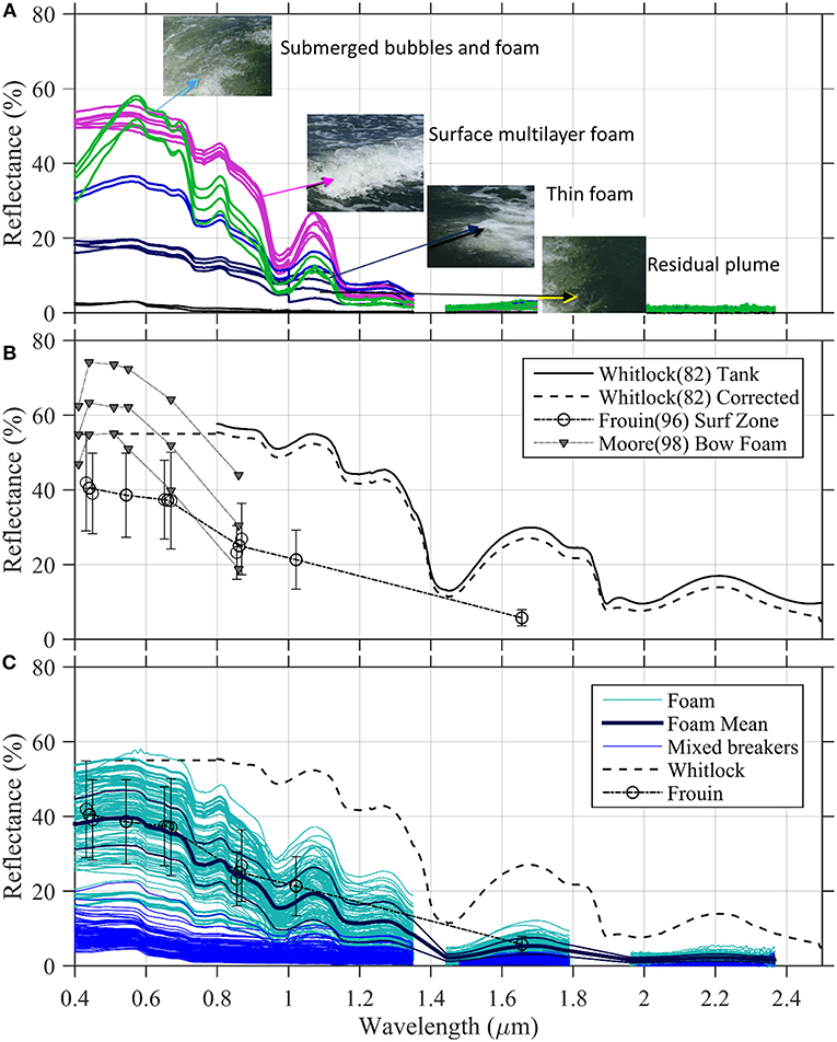
Figure 2. (A) Select examples of manufactured whitecap reflectance and the associated pictures of the sea surface. (B) Historic whitecap reflectance measured over the last 25 years from an indoor tank (Whitlock et al., 1982), bow wake from a research vessel (Moore et al., 2000) and natural breaking in the surf zone (Frouin et al., 1996). The Whitlock et al. (1982) spectrum was modeled using the published relationship to absorption by waters spectrum for wavelengths >800 nm (black line) and corrected for the reflectivity of the barium sulfate standard (dashed black line). (C) Reflectance measured in Long Island Sound, USA of intense wave breaking from a ship bow (cyan) and mixed pixels of natural waves breaking (blue) in relationship to published studies. Average whitecap reflectance is shown as the thick black line overlying the cyan measurements with ±1 standard deviation.
High reflectance can also occur when considerable amounts of bubbles are produced at depth (Figure 2A, green lines). In comparison to breaking waves, however, the spectral shape in visible wavelengths is different likely due to multiple scattering within the water. The waters of Long Island Sound have considerable blue-absorbing colored dissolved organic matter and detritus causing waters with submerged bubbles to be less “white” in visible wavelengths and have a more green-peaked reflectance spectrum (Figure 2A, green lines). The spectra appear as amplifications of the background water reflectance (Stramski and Tegowski, 2001). However, these spectra from deep bubbles produced from a submerged engine are not necessarily representative of normal surface wave breaking and are not considered further in this analysis.
Reflectance of thin layers of foam and residual bubble plumes diminish with similar spectral shapes to the breaking waves (blue lines, Figure 2A). Of note, our field measurements of thin foam produced by whitecaps had ~18% reflectance in the visible wavelengths was nearly equivalent to 22% in visible wavelengths used as an average whitecap reflectance in current atmospheric correction algorithms. This value was estimated by Koepke (1984) who showed that reflectance varied from 20 to 55% upon initial wave breaking to 3–10% after 10 s and an time-averaged effective reflectance of whitecaps of 22% was derived. However, there is considerable uncertainty in those values because a radiometer was not used to measure reflectance but rather a measure of film density was used assuming that the maximum reflectance was 55% (Whitlock et al., 1982) and presuming background water reflectance was equal to Fresnel reflectance of sun glint. Moreover, simply averaging the reflectance over the time-course of a breaking wave may not accurately reflect the physics of wave breaking. The spectral shape of the wave can change as the wave transitions to Stage B with more bubble plumes and more of the underlying water color contributes to the color (Moore et al., 2000).
Our measurements of both natural and manufactured foam are compared to other published measurements of spectral reflectance. Past studies reveal considerable variability in whitecap reflectance varying from 75 to 40% in the visible wavelengths (Figure 2B). Many of the past measurements were conducted with multi-spectral instruments that covered discreet bands within the visible and near-infrared (NIR). Frouin et al. (1996) studied the visible and NIR of sea foam found in the turbulent surf zone. As shown in Figure 2B, sea foam reflectance was found to monotonically decrease into the near infrared wavelengths due to enhanced water absorption in these wavelengths decreasing by 40% at 850 nm, 50% at 1020 nm, and 85% at 1650 nm (Frouin et al., 1996). Measurements by Moore et al. (1998) of foam produced by the bow of a large ship have higher reflectance values (50–75%) and a more green-peaked spectrum in visible wavelengths. However, a similar decay in reflectance out to 860 nm near infrared wavelengths was found by Moore et al. (1998), as well as a decrease at 670 nm compared to blue-green wavelengths. These peaked spectra are closer to the ones produced by deep submerged bubbles in Figure 2A and this may be a result of the type of foam and deeper bubbles produced by the wake of a large ship.
Whitlock et al. (1982) was the first to measure the full spectral reflectance of different layers of foam from 350 to 2700 nm. The reflectance profiles are generally spectrally flat in visible wavelengths with a maximum of 60% and higher reflectance into the NIR and SWIR than observed in other studies (Whitlock et al., 1982). Reflectance from 500 to 800 nm shown in Figure 2B (black line) are from Whitlock et al. (1982 Figure 2A) and derived from the polynomial fit with absorption by water at wavelengths >800 nm (Whitlock et al., 1982, Equation 1). Whitlock et al. (1982) also found a strong relationship between the absorption by pure water at >800 nm and the measured whitecap spectrum and noted reflectance minima at 1,500 and 1,900 nm that correspond to absorption peaks of clean water. A fourth order polynomial model was developed to model the whitecap reflectance from absorption by water. A similar approach was used in this study, as developed below.
While the work was seminal, several problems are evident in the Whitlock et al. (1982) study. First, the values of water absorption from 400 to 800 nm, shown in Figure 2B of Whitlock et al. (1982), are roughly an order of magnitude higher than the cited values (Smith and Baker, 1981). This could explain why the polynomial model of Whitlock does not extend into visible wavelengths. Secondly, the values are quite high in NIR and SWIR compared to other datasets. A reference standard of barium sulfate (EASTMAN 6080 paint) reference surface was used and reported to have 94–99% reflectivity out to 2,000 nm with no correction. While this non-luminescent coating yields reflectance values of 95–98% over the wavelength region from 300 to 1,200 nm, it is spectrally varying from 60 to 80% out to 2,500 nm. Hence, the Whitlock et al. (1982) values are too high and these were “corrected” based on the estimated spectral reflectance of this coating (Figures 2B,C dotted line), although the amount and condition of the coating are not known. However, even with this correction, the Whitlock values are much higher in the NIR and SWIR compared to field measurements made in natural seawater, which could also be due to artifacts in the tank setup that lead to further uncertainty in the NIR and SWIR values of Whitlock et al. (1982).
Two different datasets are provided in Figure 2C and compared to the Whitlock and Frouin measurements. The blue lines in Figure 2C represent measurements of mixed pixels of naturally produced foam, bubbles and background water from rolling breakers obtained close to the water surface from a small boat. The cyan lines represent a compilation of measurements made over bright thick foam at the sea surface mostly generated from a boat wake produced by the shallow-draft 11-m long R/V Lowell Weicker. These waves have considerably larger reflectance than the 22% average used in the standard algorithm for average open ocean waves and average reflectance of ~40% in visible wavelengths. Reflectance dips are prominent particularly at 750, 980, and 1,150 nm which have enhanced liquid water absorption, a result of multiple scattering in and around the bubbles and foam. The cyan lines tend to follow the range measured by Frouin et al. (1996) despite the fact that the measurements were taken over very different types of water and generated foam (i.e., Long Island Sound vs. San Diego surf zone). A mean from our spectrum is highlighted in the thick blue line (Figure 2C) and reveals a similar decay in NIR wavelengths to Frouin et al. (1996) but with more spectral features in the NIR and SWIR.
Model of Average Whitecap Reflectance From Water Absorption
Similar to the approach followed by Whitlock et al. (1982), we modeled the average whitecap spectrum (Figure 2C thick black line) using a polynomial fit to water absorption. The relationship between liquid water absorption and whitecap reflectance is predicted from visible to SWIR wavelengths. The high reflectance corresponds to low water absorption primarily in visible wavelengths and the low reflectance corresponds to high water absorption in NIR and SWIR. A second order polynomial fit to the data explains much of the inverse relationship (Figure 3A, R2 = 0.975), but misses the complexity of the shape. A simple third order polynomial on the log-transformed water absorption is a near match to the average whitecap reflectance spectrum across the visible to SWIR wavelengths (Figure 3B):
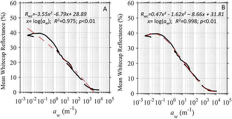
Figure 3. Relationship between absorption by seawater on a logarithmic scale (Rottgers et al., 2011) and the average whitecap reflectance measured here fit with a (A) second order and (B) third order polynomial.
For wavelengths < 400 nm, there is a slightly lower reflectance spectrum than that predicted by water absorption (Figure 3B). This is likely due to absorbing constituents within the water like colored dissolved organic matter and more investigation is needed to accurately explore whitecap reflectance in the ultraviolet wavelengths.
The whitecap reflectance reveals troughs that occur in local liquid absorption maxima evident in the water absorption spectrum (Figure 4). These troughs are centered around 600, 756, 970, 1,198, 1,448, and 1,932 nm and are specific to water in the liquid form, as the maxima shift when water is in solid or vapor form. For example, the snow community uses the shift from 1,030 nm of the imaginary index of refraction (i.e., absorption) of pure ice to 970 nm for liquid water in algorithms to estimate the liquid water content of melting snow (Green et al., 2002). This same absorption feature is shifted to 940 nm for water vapor and is often a channel used for estimating perceptible water vapor and other atmospheric remote sensing applications (Ningombam et al., 2016; Ibrahim et al., 2018). Hence, the liquid absorption features detectable in the whitecap reflectance measured at the sea surface may wholly or in part be obscured by water found in various forms in the atmosphere due to the close and overlapping absorption bands of water in its various forms (see analysis in Section Whitecap Modeling for the PACE sensor below).
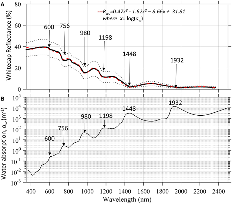
Figure 4. (A) Average whitecap reflectance measured for intense breaking waves with ± 1 standard deviation reveals local reflectance troughs corresponding to (B) Local maxima in liquid water absorption (Rottgers et al., 2011).
Radiative Transfer Modeling of Whitecaps
The close relationship between whitecaps and liquid water absorption implies that these can be tied within the theoretical framework of radiative transfer modeling. Indeed whitecaps belong to a broad class of strongly multiple-scattering media where the volumetric concentration of bubbles is >70% (Kokhanovsky, 2004). Radiative transfer modeling typically applies to media with a low concentration of scatterers (<1% by volume), but progress has been made in the development of the phenomenological optics of whitecaps (Kokhanovsky, 2004; Ma et al., 2015). Zege et al. (1991) provide a radiative transfer model of closely packed optical foam. Kokhanovsky (2004) furthered this work to provide a simple model semi-infinite foam, but notes this can extend to the case of finite foamed media having a large optical thickness (which is similar to a whitecap). Whitecap reflectance has been related to the liquid bulk water absorption (aw), the reflectance function for a single scattering albedo of 1 (i.e., a non-absorbing media) (Ro), and a spectrally neutral constant (h) through the following relationship valid for a semi-infinite foam layer (Kokhanovsky, 2004):
The values for b and Ro can be fit to experimental data or solved based on the physics using the liquid fraction (l), the average diameter of the bubbles (d), the constant B related to the real part of the index of refraction of liquid water, and Q related to the illumination conditions and observation geometry.
However, more research is needed to fully interpret these parameters in the scope of breaking waves and foam on the sea surface. Kokhanovsky (2004) was able to match the Whitlock et al. (1982) spectrum at wavelengths >800 nm only by adding a component to water absorption equivalent to 0.000270 μm−1, three orders of magnitude higher than values found in the ocean (e.g., ~0.270 m−1). If typical values of water absorption are used in Equation (8), then the modeled spectrum is much higher in magnitude and the water absorption features are much more dramatic than that of a typical whitecap (Figure 5, blue line). To achieve the appropriate magnitude of whitecap reflectance, the Ro parameter can also be tuned to <1.0, which may account for some loss of energy as light passes through the air-water interface (Kokhanovsky pers. comm.). If we fit our whitecap spectrum (Figure 5 black line) with Equation (8) using non-linear least squares, we arrive at Ro = 0.36 and b = 10.3 mm (Figure 5 red dotted line, R2 = 0.97, RMSE = 0.0311).
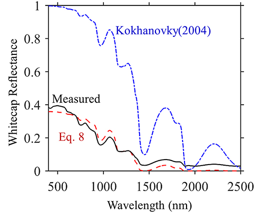
Figure 5. Radiative transfer theory of whitecaps (Kokhanovsky, 2004) was modified from the high published values (blue line) to fit the average whitecap reflectance (black line) by tuning the parameters in Equation 8. The best fit (dotted red line) had an Ro = 0.36 with a spectrally neutral constant b of 10.3 mm that translates to an equivalent water thickness of ~0.01 mm and a mean bubble size range from 0.16 to 1 mm.
This h can be deconstructed to estimate the amount of liquid water and size of bubbles using (Equation 9) above. The parameter B was assumed to ~2.3 for media similar to whitecaps following from Kokhanovsky (2004). The parameter Q can be calculated as follows (Zege et al., 1991):
Given an incidence angle of 20° equivalent to the solar zenith angle and a nadir observation angle and presuming Ro is 0.36 (modeled), Q is 4.40 for our measurement. With these assumptions, we can solve for the equivalent water thickness of 0.099 mm for our average whitecap reflectance. The question arises whether this parameter can be further decomposed into realistic liquid water content and bubble size distributions of a breaking wave.
Bubble clouds near the surface may be crudely separated into short-lived high void-fraction plumes of large bubbles close to the surface embedded in a more slowly varying low-void fraction background field of smaller bubbles extending to greater depths (Melville, 1996). Technology has allowed for better visualizations of breaking wave processes at small scales within the surface ocean (Blenkinsopp and Chaplin, 2007, 2011). As highlighted in Figure 6, modified from Blenkinsopp and Chaplin (2007, 2011), the fraction of air or “void fraction” is much larger in the above water whitecap compared to the underlying submerged bubble plumes. If we infer that the reflectance of the whitecap is largely from the above-water portion of bubbles, the void fractions range from 60 to 99%. The liquid water fraction is the non-air fraction and would then range from ~1 to 40% (Melville, 1996; Blenkinsopp and Chaplin, 2007). Using this range for l in Equation (9), the average bubble diameter, d, contributing to the measured whitecap reflectance would range from 0.16 to 1 mm.
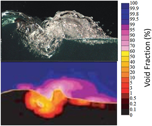
Figure 6. High resolution cross-section of a breaking wave in a laboratory setting and the corresponding void fraction measured using an optical fiber detection probe (Blenkinsopp and Chaplin, 2007). As it is difficult to define the free surface in a turbulent aerated flow, the 50% void fraction contour is used to approximate the position of the free surface. Published with permission from C. Blenkinsopp.
Bubble size distributions are generally measured on the submerged plume within the water column. They generally follow a power law distribution (Blenkinsopp and Chaplin, 2010; Randolph et al., 2014; Deane et al., 2016). However, determining an average bubble diameter is dependent on the size range of bubbles under consideration and the technology used to assess their sizes. For example, acoustics tend to measure a larger size range than afforded by optical methods (Randolph et al., 2014). Most of these approaches are designed to measure bubbles plumes within the water and not surface expressions of foam. However, the larger range of diameter (1 mm) found here is consistent with measurements of bubbles sizes in plumes of breaking waves (e.g., Deane et al., 2016). More experimental research is needed to further constrain the radiative transfer model and underlying assumptions. The ultimate objective would be to use optical measurements of whitecaps from satellites to further elucidate the physics of wave breaking and gas exchange under different environmental conditions across the world ocean.
Estimation of Whitecap Coverage With Known Background Reflectance
Various components of breaking waves can contribute to the reflectance (Frouin et al., 1996). The simplest formulation and the one currently employed by ocean color correction algorithms is to treat the ocean as a mixed pixel where the whitecap component has a constant reflectance, Rf, and covers a fraction of the sea surface, A, and the remaining fraction of sea surface is comprised of a constant background water-leaving reflectance, Rw, such that:
Even though area-weighted averages should be used for the whitecap and white-cap free areas in atmospheric correction routines (Gordon, 1997), the (1-A) term is not explicitly incorporated in retrievals of water-leaving reflectance. Presumably this introduces little error under most wind regimes where whitecap fraction, A, is very low and when considering standard 1-km ocean color pixels that average over a large ocean footprint. However, as satellite spatial resolution becomes smaller, the fraction of whitecap within a pixel can become higher and this error would need to be rectified. The fractional whitecap coverage in pan-sharpened Landsat or Sentinel 2 images (e.g., Figure 1A) can vary from 0 to nearly 1 within a given scene. For this modeling, A is derived as a “whitecap factor” rather than a whitecap fraction since it can be applied to an individual pixel and has no spatial dependence.
A whitecap can also be treated as semi-transparent where there is a contribution from the water layer below. Such a two-layer system can be modeled by the following equation which considers reflectance from the foam layer and an approximation of the water layer which has been attenuated by the overlying foam layer. The optical properties of diffusing materials (Duntley, 1942) can be used to consider a layered whitecap system water the water-leaving reflectance is attenuated by the overlying foam layer (Frouin et al., 1996), such that:
However, it should be noted that the contribution of the water-leaving radiance is negligible when overlain by a thick surface foam, as measured here. The utility of this formulation would only be significant when there is a thin foam and the presumed Rf is low.
Hence, another way to consider the problem is to specify separate contributions from thick foam, as well as a semitransparent thin foam/bubble layer overlying the background water, which can also contain submerged bubbles, and potentially submerged bubbles without surface foam (Zege et al., 2006; Randolph et al., 2014). This would imply a fraction covered by the opaque whitecaps (A1) and another fraction that may be covered by semitransparent layer (A2). If we presume that the thinner foam has the same spectral shape but reduced magnitude when compared to thick foam (e.g., Figure 2A), then the thin foam could be written as a fraction, F, of Rf and the formulation would look like:
These 3 different models (Equations 10–12) were tested using a time series of reflectance measurements made over natural mixed pixels of background, bubbles, and whitecaps (e.g., rolling breakers) (blue lines in Figure 2C). Model parameters were fit to 88 different spectra using non-linear least squares to the total reflectance measured between 400 and 1,800 nm presuming a known background reflectance of water, Rw, and the average whitecap reflectance from Equation (7) (Figure 4A). The simplest model was able to capture the spectral shape from mixed pixels with lots of foam to those just above the background, as illustrated by a range of selected spectra shown in Figure 7A. The modeled retrieval of total reflectance showed good correspondence across all wavelengths (Figure 7B) with and R2 of 0.96 and a slope of 0.98. The MAPE estimate for each wavelength (Figure 7C) shows that the model achieves an average of 18.5% across the spectrum and 9.0% in visible wavelengths (400–700 nm). Application of the second model (Equation 13) which includes a term for semi-transparent whitecap provided little improvement in fit with an average MAPE of 18.69% and 8.27% in visible wavelengths. As mentioned earlier, this is likely because the whitecap reflectance is high and the contribution of the water-leaving radiance is negligible when overlain by a thick surface foam. The third model (Equation 14) allows for a thinner foam layer, but has more free parameters to fit (F, A1, and A2) and unique solutions were difficult to constrain. The model seemed to overfit either A1 or A2 with either fractions of 0 or 1.0. Additionally, the complexity of this model did not significantly improve the fit to the measured spectra and the MAPE was 18.20 and 8.85% in visible wavelengths. Hence, the simplest model (Equation 13) captured the large range in reflectance from mixed pixels, particularly at higher whitecap factors. This provides further evidence that the mixed pixel behaves in a linear manner and the retrieved effective whitecap factor is able to account for different thicknesses of foam on the sea surface.
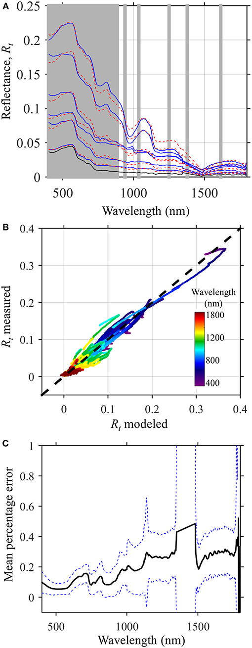
Figure 7. (A) Reflectance measurements of selected mixed pixels (blue lines) of whitecaps and background reflectance (black line) measured in Long Island Sound, USA and a modeled fit using the average whitecap reflectance (Equation 7) and a simple mixed pixel model (Equation 12). The gray regions highlight spectral bands proposed for the PACE mission. (B) spectral fit of the mixed pixel model (Equation 12) showing measured and observed reflectance colored by wavelength for 88 spectra. (C) mean percentage error and ± 1 standard deviation by wavelength varied from 8% in visible wavelengths to 20% in shortwave infrared wavelengths.
Estimating Whitecap Coverage With Unknown Background Reflectance
The above exercise illustrates that a simple model is capable of reproducing the total reflectance from a mixed pixel of foam and background reflectance using the average whitecap reflectance spectrum (Equation 7). The retrieved whitecap factor is an “effective” whitecap coverage that incorporates different levels of foam and bubbles within the pixel varying from 0.01 to 1. With this parameter, the contribution of whitecaps can be removed from the mixed pixel in order to retrieve an estimate of the background water-leaving reflectance that is needed for implementation of ocean color products. In this section, we consider different algorithms that could be used to retrieve to the effective whitecap factor assuming that the background reflectance is not known.
Following from the previous section, an iterative procedure could be implemented to retrieve both the fractional whitecap coverage and the background reflectance with a constant whitecap reflectance by adjusting the shape of background reflectance and fractional whitecap coverage with an optimization routine. Constraints could be applied such that background reflectance is retrieved within the scope of known water-leaving reflectance shapes. Such an optimization, however, may be sensitive to other components of atmospheric correction, such as the choice of aerosol models and removal of diffuse and direct sea surface reflected solar radiance. Hence, the average whitecap reflectance (Equation 7) could be straightforwardly incorporated into existing models that solve both the water and atmospheric components simultaneously (Stamnes, 2003; Fan et al., 2017) or atmospheric correction schemes that rely on spectral matching and optimization (Steinmetz et al., 2011).
Other atmospheric correction algorithms from ocean color satellites are stepwise and incorporate an independent determination of the contribution of whitecaps to the total radiance at the top of the atmosphere (Gordon, 1997; Bailey et al., 2010; Ibrahim et al., 2018). To assess the parts of the spectrum most useful for discrimination of whitecap factor, a correlation matrix was constructed to assess how combinations of different wavelengths could be used to predict whitecap factor, A. A Normalized Difference Index (NDI) was used which is the difference between two wavelengths normalized by the sum of the wavelengths (Figure 8; Dierssen et al., 2015). The normalization constrains the index to values between −1 and 1 with 0 indicating no difference and can be used to isolate narrowband features within a hyperspectral signal. Using this index, regions of highest correlation are localized in discrete wavebands and primarily include water absorption bands at 750 nm, 900–980 nm, and 1,100–1,300 nm. Specifically, a higher effective whitecap factor resulting either from more whitecaps in a pixel or more intense breaking waves are expressed as greater reflectance troughs in the liquid water absorption bands highlighted in Figure 4 (600, 756, 980, 1,198, 1,448 nm).
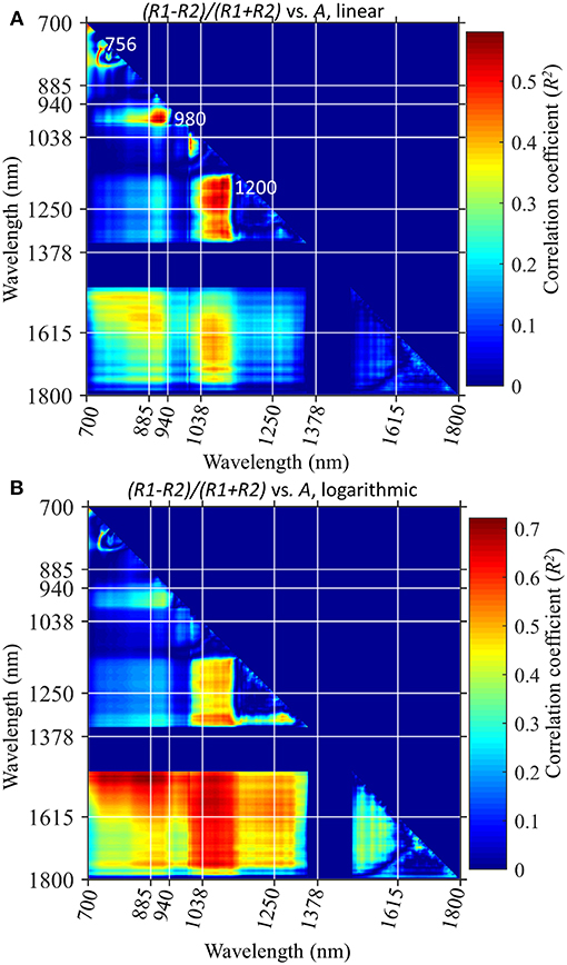
Figure 8. Correlation matrix of normalized difference index calculated using pairs of wavelengths from near infrared through the shortwave infrared in relationship to the derived effective whitecap factor (A) from Equation 12. The colors represent the correlation coefficients derived on a (A) linear scale with NDI vs. A; (B) logarithmic scale with log(NDI) vs. log(A). Selected wavelengths proposed for the PACE mission are highlighted in white.
The initial correlation was done on a linear scale, but a logarithmic scale is more appropriate given the distribution of whitecap factor and the radiance values (Figure 9). Areal-averaged whitecap factors can range over three orders of magnitude roughly from 0.001 to 0.1 (Brumer et al., 2017). Using a logarithmic distribution in the correlation analysis (Figure 8B), the correlation coefficients are higher and the SWIR features are more prominent compared to the linear fit. The amount of reflectance in SWIR bands (1500–1800 nm) is found to be highly correlated to the whitecap factor with R2 > 0.90 for some combinations of wavebands (Figure 8B). While these SWIR bands are not specific liquid water absorption features, the enhanced reflectance in SWIR wavelengths can be important predictors of whitecap contribution and can potentially interfere with aerosol and glint atmospheric correction methods (see Section Whitecap Modeling for the PACE sensor below).
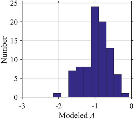
Figure 9. Histogram of the derived effective whitecap factor (A) from mixed pixels of natural breaking waves using Equation 12 reveals the logarithmic distribution of A ranging from −2 to 0 in logarithmic space or 0.01 to 1.
Whitecap Modeling for the PACE Sensor
This analysis focuses on the proposed bands for incorporation in the PACE OLI sensor which include hyperspectral bands from 350 to 890 nm in 5 nm increments with additional largely heritage NIR/SWIR bands at 940, 1,038, 1,250, 1,378, 1,615, 2,130, 2,260 nm. The 1,378 nm channel is not included further in this analysis, because the atmosphere highly attenuates radiance in this band and reflectance at the sea surface is not measurable under most conditions. The PACE OLI sensors misses many of the NIR/SWIR bands related to liquid water absorption such as features around 980 and 1,200 nm. However, PACE is poised to be hyperspectral into the NIR and this analysis shows narrowband information in the 730–800 nm region that are related to the liquid water absorption features at 756 nm. In addition, the 1,038 nm band also may provide information on whitecap, although this region is likely also used for aerosols and sun glint extrapolations.
If we presume that the sea surface is a mixture of pure whitecap with whitecap-free background reflectance, then a simple linear mixing model could be developed to quantify the depth of the reflectance trough for different liquid water absorption bands. For the data collected here, the depth of the trough related to liquid water absorption is related to the derived whitecap factor for the 980 and 1,200 nm features. A baseline subtraction approach (also referred to as continuum removed) has proven to be robust for many environmental remote sensing applications (Clark, 1999; Dierssen et al., 2015; Khan et al., 2017; Garaba and Dierssen, 2018) and is explored here (Figure 10). The water absorption features at ~750 nm is not a robust indicator when the whitecap factor is low. However, the absorption features at 980 nm and 1,200 nm are well-correlated to whitecap factor across several orders of magnitude (0.02–1) and have little bias and fairly low error (Figure 10). Similar results are found for a simple band difference algorithm (Table 1). The NDI does not perform as well in predicting whitecap factor for any of these spectral regions because the normalization to the sum of the reflectance values tends to obscure the relative differences (Table 1).
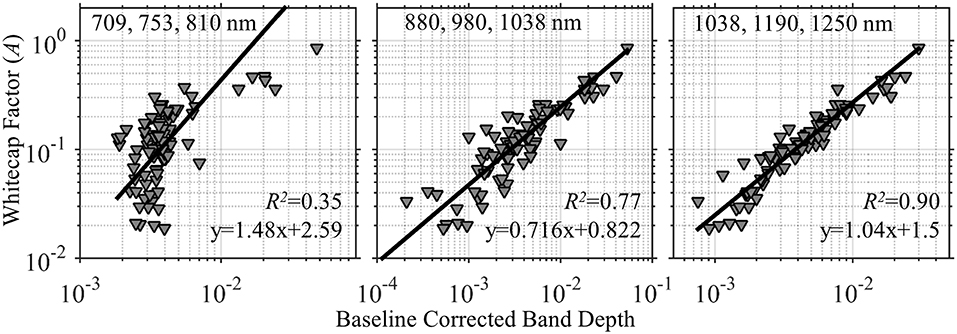
Figure 10. Various models to derive effective whitecap factor (A) from baseline corrected band-depths calculated using different combinations of 3 wavelengths (see Table 1 for additional statistics). Band depths at the liquid water absorption features centered at 980 and 1,200 nm are highly correlated to the whitecap factor on a logarithmic scale. These bands are not proposed to be part of the PACE mission.
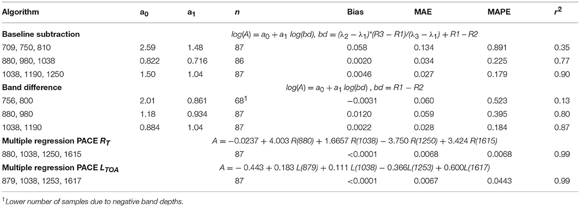
Table 1. Statistical results from various algorithms to estimate the whitecap factor, A, from spectral reflectance at the sea surface and at sensor radiance.
While these liquid water absorption bands are not currently part of the PACE mission, this analysis suggests their addition, particularly 980 and 1,200 nm, could be valuable for predicting whitecap factor and other sea surface applications. High correlations can also be found with a multiple linear regression for select bands in the far NIR/SWIR including 880, 1,038, 1,250, and 1,615 nm (Table 1). As discussed earlier, whitecaps elevate the reflectance in the NIR/SWIR above background and the amount of signal within these bands is a good predictor of the fractional whitecap coverage. The 940 nm band was excluded from the regression analysis because this band varies with atmospheric water vapor absorption. The generality and applicability of these algorithms broadly across different oceanic regimes and atmospheric conditions remains to be tested.
Many of the features unique to whitecaps may be part or wholly obscured by the intervening atmosphere. Hence, a simple transformation was conducted to determine whether the signal observed at the sea surface could “potentially” be observed at the Top of the Atmosphere (TOA). This transformation is for a single atmospheric condition with a realistic set of aerosols and atmospheric gases and does not consider the impact of highly scattering waters on atmospheric processes (e.g., multiple scattering). It provides a glimpse of what a satellite might observe over whitecap-enhanced waters in the bands expected on PACE. The TOA radiance is nearly an order of magnitude higher in visible wavelengths, but the two datasets become closer in magnitude into the NIR and SWIR wavelengths (Figure 11A). The separate contribution of Rayleigh (Lr) and aerosols (La) are shown in comparison to a whitecap pixel (Lw maximum) and an unimpacted background pixel (Lw minimum) (Figure 11B). Pixels completely covered by whitecaps (A = 1) contribute more radiance than aerosols at the TOA from visible to 1,615 nm. This would not be observed on PACE, however, given the large spatial footprint of 1 km and typical values of A < 0.1. Another feature of note is that the changes in radiance are less sensitive to whitecap factor at the top of the atmosphere having steeper slopes (Figure 11C) compared to reflectance at the sea surface (Figure 11D). This could impact the ability to retrieve low whitecap factors common to open ocean conditions from TOA radiance. The impact of different atmospheric conditions will also need to be explored.
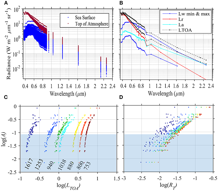
Figure 11. (A) An example of radiance (W m-2 μm−1 sr−1) at the sea surface and the top of the atmosphere in bands similar to those proposed to be on the PACE mission estimated from 88 spectra measured over different mixtures of whitecap and background including direct and diffuse reflected skylight for a single marine atmosphere. (B) Individual contributions to the top of the atmosphere radiance (LTOA) from Rayleigh (Lr), aerosol (La), and the water signal (Lw) over background (min) and whitecap-covered (max) sea surfaces. (C) Relationship between the logarithm of LTOA (from Panel A) and the effective whitecap reflectance for the near infrared (NIR) and shortwave infrared (SWIR) bands. (D) Same analysis as in (C) But for total reflectance measured at the sea surface.
Gordon (1997) writes that “area-weighted averages” of the whitecap-covered and whitecap-free areas of the surface should be considered in the formulation for atmospheric correction (Gordon, 1997). However, current correction routines do not incorporate the (1-A) fraction for the remaining signal emanating from the sea. This may not introduce much error in the current implementation of the whitecap correction routine, which only considers low fractions of whitecaps (A < 0.02). The formulation by Gordon (1997) also presumes that reflection of the direct and diffuse skylight would be the same over whitecap-covered and background waters; however, seas with breaking waves and foam do not reflect light in the same way as flat or wind-ruffled seas. Hence, the area-weighted average of whitecap-free sea surface should potentially include the direct beam (sun glint, Lg) and diffuse skylight (Ld) in addition to the water-leaving component. A modification of the traditional algorithm for conducting atmospheric correction (Gordon, 1997) is proposed that explicitly incorporates the fraction of whitecap-covered and whitecap-free areas following:
where t is the diffuse and T is the direct transmittance of the atmosphere. This equation separates the component of the diffuse reflected skylight, Ld, from the computed Rayleigh radiance and includes it as part of the water signal. This allows for true validation of the atmospheric correction approach, whereby values of Lg, Ld, Lw, and Lf can be individually measured and compared to those derived from the atmospheric correction algorithm.
The εobs used to estimate the aerosol model for atmospheric correction purposes was evaluated at different combinations of NIR and SWIR wavelengths (Figure 12). As shown in Figure 12A, εobs is quite insensitive to whitecap factor using the NIR wavebands of 753 and 869 nm. The liquid water absorption feature at 753 nm compensates for the enhanced reflectance due to the whitecaps. However, the SWIR wavelengths at 1,253, 1,617, and 2,132 nm do not incorporate the liquid water features and εobs is dependent on the whitecap factor with different combinations of SWIR bands. No correlation is found between whitecap factor and εobs(753,869), while the correlation coefficients are 0.54 and 0.36 for εobs(1,253,1,617) and εobs(1,617,2,132), respectively. The range in εobs is large for Figures 12B,C and would result in different aerosol spectral models and variable amounts removed from visible wavelengths, even though the atmospheric properties and water-leaving reflectance were the same.
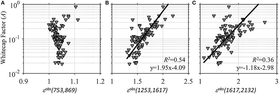
Figure 12. Estimates of the observed epsilon εobs for the two specified wavelengths (Equation 5,6) used in the selection of aerosol models is shown in relationship to the logarithm of effective whitecap factors. The εobs calculated using the near infrared (753 and 869 nm) is nearly invariant of whitecap factor (A) compared to the ratios calculated with shortwave infrared wavelengths (1,253, 1,617, and 2,132 nm) (B,C).
Conclusions and Outlook
Field measurements of the spectral reflectance of whitecaps are challenging to collect due to the many types and stages of whitecaps, the rapid time scale on the order of seconds, the changing contributions of foam and still water, and potential contamination from reflectance of sun and skylight. Reflectance of whitecaps also varies with the type of breaking wave (e.g., rolling breakers and plunging breakers) and the layers of foam and bubbles produced (Frouin et al., 1996; Moore et al., 2000). This was evident in the early measurements of Koepke (1984) who demonstrated the time dependent-variability of the reflectance of breaking waves averaging around 22%. However, that study was limited to simple photography and the spectral shape was presumed to be flat, with later studies highlighting the reduction in reflectance in the NIR (Frouin et al., 1996). Few studies have evaluated whitecap reflectance into the SWIR and at the spectral resolution necessary for atmospheric correction of hyperspectral sensors (e.g., the proposed PACE).
This study builds upon past research to present new whitecap measurements from 350 to 2,500 nm that are useful not only for atmospheric correction, but for sensor design in terms of waveband selection in NIR and SWIR wavelengths. Our measurements in visible and NIR wavelengths are consistent in magnitude with several of the past multi-spectral measurements of whitecaps from vastly different water conditions (Frouin et al., 1996). This consistency in measurements may be a further indication of a phenomena called “turbulence saturation,” whereby the time- and space-averaged fluid turbulence in actively breaking wave crests is proposed to remain approximately constant (Deane et al., 2016). As highlighted in the radiative transfer section above, bridging the physics of wave breaking and radiative transfer (Kokhanovsky, 2004; Ma et al., 2015) is a subject requiring more intensive research and could lead to new predictive capabilities from ocean color data that include estimates of whitecap factor and the intensity of breaking wave features on the sea surface.
Similar to the pioneering work of Whitlock et al. (1982), the average whitecap spectrum is empirically related to the liquid water absorption coefficient from visible to SWIR using a third order polynomial (Equation 7). However, the new hyperspectral parameterization is proposed to be more accurate for natural breaking waves across all wavelengths compared to the laboratory study of Whitlock et al. (1982) and is now consistent from 400 to 2,500 nm. This whitecap parameterization can be easily input into radiative transfer models and various atmospheric correction schemes for ocean color imagery. In particular, the new whitecap parameterization could be input as a spectral shape in spectral matching and optimization algorithms (Steinmetz et al., 2011), which could result in improved atmospheric correction over whitecap-prone seas like the Southern Ocean. Prominent reflectance troughs in the whitecap spectrum correspond to liquid water absorption features at ~750, 980, and 1,200 nm. These absorption features are related to the intensity of breaking wave features whereby more intense foam production leads to enhanced multiple scattering by the medium (Zege et al., 1991; Kokhanovsky, 2004) and enhanced absorption in these localized bands. As shown here, the depths of the reflectance trough at 980 and 1,200 nm are highly related to the effective whitecap factor from 0.01 to 1 and could provide new means to estimate this parameter from the ocean color image.
The liquid water absorption features highlighted here are not unique to reflectance features of whitecaps and can occur from other types of floating or suspended constituents at the sea surface. For example, various types of floating vegetation including the macroalgae Sargassum sp. and floating leaf debris of seagrass (i.e., seagrass wrack) can contain these same water features out to nearly 2,500 nm (Dierssen et al., 2015; Hu et al., 2015). For example, the liquid water absorption feature at ~980 nm has been used for terrestrial applications to map drought within plant communities (Peñuelas et al., 1997; Roberts et al., 2016). Dierssen et al. (2015) related the dip in reflectance at 980 nm to the age of floating seagrass wrack advected from coastal seagrass beds to the oligotrophic ocean. Highly turbid sediment plumes also have similar dips in reflectance at these same liquid water absorption bands up until 1,150 nm (Knaeps et al., 2015). Differentiating highly scattering media at the sea surface, such as sediments, floating vegetation and whitecaps, is possible using spectral characteristics that are unique to each constituent (e.g., red edge of vegetation) (Dierssen et al., 2006) and will be considered in future research.
The “effective” whitecap factor, A, derived here is based on optical reflectance rather than the traditional interpretation of whitecap fraction as an aerial average of bright features observed over a large area of the sea surface. In photographic methods commonly used to estimate whitecap fraction, the threshold of what is considered a “bright feature” is not easy to standardize and large uncertainty exists in derivation of whitecap fractions (Brumer et al., 2017). The “effective” whitecap factor (Equation 12) is the fraction of a standard whitecap reflectance (e.g., Equation 7) that accounts for enhancements in spectral reflectance of the sea surface above the background reflectance. Since A is optically derived, it is better suited for atmospheric correction techniques because it specifically incorporates different levels of foam and bubbles associated with breaking waves and can incorporate small enhancements in reflectance that may not be observable with the eye or photographic systems (Randolph et al., 2017). Moreover, unlike the whitecap fraction parameterized with wind speed measurements, no spatial extent is implicit to A and “effective” whitecap factor can apply to reflectance measurements at any spatial scale on the sea surface. For a large pixel, A can be related directly to the whitecap fraction on the sea surface. For a small pixel, A can be higher than 1.0, if reflectance is greater than the average whitecap reflectance used in the model, and A can be lower than the limit used here of 0.01.
The simple whitecap model (Equation 12) is consistent with the standard model used in most atmospheric correction routines where the sea is treated as a mixed pixel comprising both whitecap and background reflectance (Gordon and Wang, 1994). Gordon (1997) specifically states that “area-weighted averages” of the whitecap-covered and whitecap-free areas of the surface should be considered, but the terms describing the area-weighted averages, specifically A and (1-A), are missing from the standard equation (Gordon, 1997, Equation 5). Without explicitly including these terms, the standard model is commonly misinterpreted as enhancements or augmentations in reflectance above a background reflectance (Equation 1). To clarify this misconception, these terms are explicitly added to the atmospheric correction equation in Equation (15). Incorporating these terms is especially important for satellites with smaller footprints and when considering an “effective” whitecap factor as described above (Thompson et al., 2015; Bender et al., 2018). In addition, the new formulation considers the reflectance from whitecap-free areas of the sea surface to include all contributions of sea spectral reflectance, including sun glint, and diffuse reflected skylight. Current models include a wind-roughened estimate of the diffuse reflected skylight in the Rayleigh component of atmospheric correction (Gordon, 1997; Ibrahim et al., 2018), which is challenging to validate. Enhanced surface roughness, which is directly linked to the generation of whitecaps and air bubble entrainment and to the formation of sea spray as significant aerosol contribution in the lower atmospheric layer, will challenge the atmospheric correction performance and in turn will affect the estimates of whitecap factor (Hieronymi, 2016).
Errors in treating whitecap reflectance for atmospheric correction of satellite imagery, particularly at high winds, are generally accounted for in the aerosol model. Specifically, any enhancement that is not removed as a whitecap is added to the aerosol reflectance in the NIR/SWIR and can impact the retrieved spectral dependence of the selected aerosol model. Even though the selected aerosol concentration and type may be inaccurate, the amount of reflectance that is subtracted may still be approximately correct to retrieve accurate water-leaving reflectance across the visible. If the PACE mission aims to improve retrievals of both aerosols and water-leaving reflectance, however, then better treatment of whitecaps is needed to ensure that errors are not propagated into the retrieved aerosol or water-leaving reflectance values. Here, the εobs used for aerosol model selection was calculated using NIR wavelengths of 753 and 869 nm and found to be quite invariant to changes in the effective whitecap factor. In contrast, εobs calculated for SWIR wavebands (i.e., 1,253, 1,617, and 2,132 nm) was highly variable with whitecap factor. A more thorough analysis of how whitecaps impact top of the atmosphere radiance and aerosol modeling under a variety of environmental conditions will be important for estimating uncertainties of parameters derived from future satellite missions, particularly in whitecap-prone regions like the Southern Ocean. Alternative methods for estimating whitecaps may also be feasible such as using depolarization characteristics of whitecaps or the use of space-based lidars (Hu et al., 2008; Hieronymi, 2016).
Rather than considering whitecaps a contamination to ocean color imagery, these results point the way forward to new avenues of research and ocean color products that could have important implications to physical oceanographers, atmospheric scientists, and climate modelers. Wave breaking leads to enhanced air-sea transfer of gases through additional turbulence and bubble-mediated transfer (Asher and Wanninkhof, 1998). Bursting of surface bubbles injects sea spray aerosols into the atmosphere and the aerosol production flux is thought to be directly proportional to the whitecap coverage. Sea salt aerosols play an important role in the earth's radiation budget through scattering of and serve as cloud condensation nuclei influencing the microphysical and radiative properties of clouds. They are also direct scatterers of solar radiation (Andreae and Rosenfeld, 2008). Including new wavebands specific to liquid water absorption features could open the door for new applications to sea surface processes with potential ecological and climatological applications.
Author Contributions
The author confirms being the sole contributor of this work and has approved it for publication.
Funding
Funding was provided by NASA Ocean Biology and Biogeochemistry through the PACE project (NNX15AC32G).
Conflict of Interest Statement
The author declares that the research was conducted in the absence of any commercial or financial relationships that could be construed as a potential conflict of interest.
Acknowledgments
The following individuals are gratefully acknowledged for assisting in data collection: Kaylan Randolph, Shungudzemwoyo Garaba, Alexandre Castagna, Timothy Bateman and Brandon Russell. Turner Cabaniss and vessel operations at the University of Connecticut Marine Sciences are also acknowledged for providing field operations in rough seas. Amir Ibrahim and Bryan Franz provided data and methods to extrapolate reflectance values to the top of atmosphere. Thanks are extended to Alexandre Castagna, Bo-Cai Gao, Robert Frouin, Kaylan Randolph and Alexander Kokhanovsky and Martin Hieronymi for insightful conversations regarding this work. I also acknowledge Norman Kurig for providing the Landsat 8 image, Monique Albert and Magdalena Anguelova for the image of whitecap fractions and C.E. Blenkinsopp and J.R. Chaplin for the measurements of void fraction.
References
Ahn, J.-H., Park, Y.-J., Ryu, J.-H., and Lee, B. (2012). Development of atmospheric correction algorithm for geostationary ocean color imager (GOCI). Ocean Sci. J. 47, 247–259. doi: 10.1007/s12601-012-0026-2
Albert, M. F., Anguelova, M. D., Manders, A. M., Schaap, M., and De Leeuw, G. (2016). Parameterization of oceanic whitecap fraction based on satellite observations. Atmos. Chem. Phys. 16, 13725–13751. doi: 10.5194/acp-16-13725-2016
Andreae, M. O., and Rosenfeld, D. (2008). Aerosol–cloud–precipitation interactions. Part 1. The nature and sources of cloud-active aerosols. Earth Sci. Rev. 89, 13–41. doi: 10.1016/j.earscirev.2008.03.001
Anguelova, M. D., and Webster, F. (2006). Whitecap coverage from satellite measurements: a first step toward modeling the variability of oceanic whitecaps. J. Geophys. Res. 111:C03017. doi: 10.1029/2005JC003158
Asher, W. E., and Wanninkhof, R. (1998). The effect of bubble-mediated gas transfer on purposeful dual-gaseous tracer experiments. J. Geophys. Res. 103, 10555–10560. doi: 10.1029/98JC00245
Aurin, D. A., and Dierssen, H. M. (2012). Advantages and limitations of ocean color remote sensing in CDOM-dominated, mineral-rich coastal and estuarine waters. Remote Sens. Environ. 125, 181–197. doi: 10.1016/j.rse.2012.07.001
Aurin, D. A., Dierssen, H. M., Twardowski, M. S., and Roesler, C. S. (2010). Optical complexity in Long Island sound and implications for coastal ocean color remote sensing. J. Geophys. Res. 115, 1–11. doi: 10.1029/2009JC005837
Bailey, S. W., Franz, B. A., and Werdell, P. J. (2010). Estimation of near-infrared water-leaving reflectance for satellite ocean color data processing. Optics Express 18, 7521–7527. doi: 10.1364/OE.18.007521
Bender, H. A., Mouroulis, P., Dierssen, H. M., Painter, T. H., Thompson, D. R., Smith, C. D., et al. (2018). Snow and water imaging spectrometer: mission and instrument concepts for earth-orbiting cubesats. 12, 044001. doi: 10.1117/1.JRS.12.044001
Blanchard, D. C. (1985). The oceanic production of atmospheric sea salt. J. Geophys. Res. 90, 961–963. doi: 10.1029/JC090iC01p00961
Blenkinsopp, C. E., and Chaplin, J. R. (2007). Void fraction measurements in breaking waves. Proc. R. Soc. A 463, 3151–3170. doi: 10.1098/rspa.2007.1901
Blenkinsopp, C. E., and Chaplin, J. R. (2010). Bubble size measurements in breaking waves using optical fiber phase detection probes. IEEE J. Oceanic Eng. 35, 388–401. doi: 10.1109/JOE.2010.2044940
Blenkinsopp, C. E., and Chaplin, J. R. (2011). Void fraction measurements and scale effects in breaking waves in freshwater and seawater. Coastal Eng. 58, 417–428. doi: 10.1016/j.coastaleng.2010.12.006
Brumer, S. E., Zappa, C. J., Brooks, I. M., Tamura, H., Brown, S. M., Blomquist, B. W., et al. (2017). Whitecap coverage dependence on wind and wave statistics as observed during SO GasEx and HiWinGS. J. Phys. Oceanogra. 47, 2211–2235. doi: 10.1175/JPO-D-17-0005.1
Clark, R. N. (1999). “Chapter 1: Spectroscopy of rocks and minerals, and principles of spectroscopy,” in Manual of Remote Sensing, Vol. 3, Remote Sensing for the Earth Sciences, ed A. N. Rencz (New York, NY: John Wiley and Sons), 3–58.
Deane, G. B., Stokes, M. D., and Callaghan, A. H. (2016). The saturation of fluid turbulence in breaking laboratory waves and implications for whitecaps. J. Phys. Oceanogra. 46, 975–992. doi: 10.1175/JPO-D-14-0187.1
Dierssen, H. M., Chlus, A., and Russell, B. (2015). Hyperspectral discrimination of floating mats of seagrass wrack and the macroalgae Sargassum in coastal waters of Greater Florida Bay using airborne remote sensing. Remote Sens. Environ. 167, 247–258. doi: 10.1016/j.rse.2015.01.027
Dierssen, H. M., Kudela, R. M., Ryan, J. P., and Zimmerman, R. C. (2006). Red and black tides: quantitative analysis of water-leaving radiance and perceived color for phytoplankton, colored dissolved organic matter, and suspended sediments. Limnol. Oceanogr. 51, 2646–2659. doi: 10.4319/lo.2006.51.6.2646
Duntley, S. Q. (1942). The optical properties of diffusing materials. JOSA 32, 61–70. doi: 10.1364/JOSA.32.000061
Fan, Y., Li, W., Gatebe, C. K., Jamet, C., Zibordi, G., Schroeder, T., et al. (2017). Atmospheric correction over coastal waters using multilayer neural networks. Remote Sens. Environ. 199, 218–240. doi: 10.1016/j.rse.2017.07.016
Frouin, R., Schwindling, M., and Deschamps, P.-Y. (1996). Spectral reflectance of sea foam in the visible and near-infrared: in situ measurements and remote sensing implications. J. Geophys. Res. 101, 14361–14371.
Garaba, S. P., and Dierssen, H. M. (2018). An airborne remote sensing case study of synthetic hydrocarbon detection using short wave infrared absorption features identified from marine-harvested macro-and microplastics. Remote Sens. Environ. 205, 224–235. doi: 10.1016/j.rse.2017.11.023
Gordon, H. R. (1997). Atmospheric correction of ocean color imagery in the Earth Observing System era. J. Geophys. Res. 102, 17081–17106. doi: 10.1029/96JD02443
Gordon, H. R., and Wang, M. (1994). Influence of oceanic whitecaps on atmospheric correction of ocean-color sensors. Appl. Optics 33, 7754–7763. doi: 10.1364/AO.33.007754
Green, R. O., Dozier, J., Roberts, D., and Painter, T. (2002). Spectral snow-reflectance models for grain-size and liquid-water fraction in melting snow for the solar-reflected spectrum. Ann. Glaciol. 34, 71–73. doi: 10.3189/172756402781817987
Guanter, L., Kaufmann, H., Segl, K., Foerster, S., Rogass, C., Chabrillat, S., et al. (2015). The EnMAP spaceborne imaging spectroscopy mission for earth observation. Remote Sens. 7, 8830–8857. doi: 10.3390/rs70708830
Hieronymi, M. (2016). Polarized reflectance and transmittance distribution functions of the ocean surface. Optics Express 24, A1045–A1068. doi: 10.1364/OE.24.0A1045
Hu, C., Feng, L., Hardy, R. F., and Hochberg, E. J. (2015). Spectral and spatial requirements of remote measurements of pelagic Sargassum macroalgae. Remote Sens. Environ. 167, 229–246. doi: 10.1016/j.rse.2015.05.022
Hu, Y., Stamnes, K., Vaughan, M., Pelon, J., Weimer, C., Wu, D., et al. (2008). Sea surface wind speed estimation from space-based lidar measurements. Atmos. Chem. Phys. 9, 3593–3601. doi: 10.5194/acp-8-3593-2008
Ibrahim, A., Franz, B., Ahmad, Z., Healy, R., Knobelspiesse, K., Gao, B.-C., et al. (2018). Atmospheric correction for hyperspectral ocean color retrieval with application to the Hyperspectral Imager for the Coastal Ocean (HICO). Remote Sens. Environ. 204, 60–75. doi: 10.1016/j.rse.2017.10.041
Khan, A. L., Dierssen, H., Schwarz, J. P., Schmitt, C., Chlus, A., Hermanson, M., et al. (2017). Impacts of coal dust from an active mine on the spectral reflectance of Arctic surface snow in Svalbard, Norway. J. Geophys. Res. 122, 1767–1778. doi: 10.1002/2016JD025757
Knaeps, E., Ruddick, K. G., Doxaran, D., Dogliotti, A. I., Nechad, B., Raymaekers, D., et al. (2015). A SWIR based algorithm to retrieve total suspended matter in extremely turbid waters. Remote Sens. Environ. 168, 66–79. doi: 10.1016/j.rse.2015.06.022
Koepke, P. (1984). Effective reflectance of oceanic whitecaps. Appl. Opt. 23, 1816–1824. doi: 10.1364/AO.23.001816
Kokhanovsky, A. A. (2004). Spectral reflectance of whitecaps. J. Geophys. Res. 109:C05021. doi: 10.1029/2003JC002177
Lee, C. M., Cable, M. L., Hook, S. J., Green, R. O., Ustin, S. L., Mandl, D. J., et al. (2015). An introduction to the NASA Hyperspectral InfraRed Imager (HyspIRI) mission and preparatory activities. Remote Sens. Environ. 167, 6–19. doi: 10.1016/j.rse.2015.06.012
Ma, L. X., Wang, F. Q., Wang, C. A., Wang, C. C., and Tan, J. Y. (2015). Investigation of the spectral reflectance and bidirectional reflectance distribution function of sea foam layer by the Monte Carlo method. Appl. Optics 54, 9863–9874. doi: 10.1364/AO.54.009863
Melville, W. K. (1996). The role of surface-wave breaking in air-sea interaction. Annu. Rev. Fluid Mech. 28, 279–321. doi: 10.1146/annurev.fl.28.010196.001431
Monahan, E. C. (1993). “Occurrence and evolution of acoustically relevant sub-surface bubble plumes and their associated, remotely monitorable, surface whitecaps,” in Natural Physical Sources of Underwater Sound (Springer), 503–517. Available online at: https://link.springer.com/chapter/10.1007/978-94-011-1626-8_37 (Accessed September 20, 2017).
Monahan, E. C. (2008). “Whitecaps and Foam,” in Encyclopedia of Ocean Sciences, 2nd Edn, eds J. Steele, S. Thorpe, and K. Turekian (San Diego, CA: Elsevier; Academic), 3213–3219.
Monahan, E. C., and O'Muircheartaigh (1986). Whitecaps and the passive remote sensing of the ocean surface. Int. J. Remote Sens. 7, 627–642. doi: 10.1080/01431168608954716
Moore, K. D., Voss, K. J., and Gordon, H. R. (1998). Spectral reflectance of whitecaps: instrumentation, calibration, and performance in coastal waters. J. Atmo. Oceanic Tech. 15, 496–509.
Moore, K. D., Voss, K. J., and Gordon, H. R. (2000). Spectral reflectance of whitecaps: their contribution to water-leaving radiance. J. Geophys. Res. 105, 6493–6499. doi: 10.1029/1999JC900334
Ningombam, S. S., Jade, S., Shrungeshwara, T. S., and Song, H.-J. (2016). Validation of water vapor retrieval from moderate resolution imaging spectro-radiometer (MODIS) in near infrared channels using GPS data over IAO-Hanle, in the trans-Himalayan region. J. Atmosphe. Solar-Terrestrial Phys. 137, 76–85. doi: 10.1016/j.jastp.2015.11.019
Peñuelas, J., Pinol, J., Ogaya, R., and Filella, I. (1997). Estimation of plant water concentration by the reflectance water index WI (R900/R970). Int. J. Remote Sens. 18, 2869–2875. doi: 10.1080/014311697217396
Randolph, K., Dierssen, H. M., Cifuentes-Lorenzen, A., Balch, W. M., Monahan, E. C., Zappa, C. J., et al. (2017). Novel methods for optically measuring whitecaps under natural wave-breaking conditions in the Southern Ocean. J. Atmosphe. Ocean. Technol. 34, 533–554. doi: 10.1175/JTECH-D-16-0086.1
Randolph, K., Dierssen, H. M., Twardowski, M., Cifuentes-Lorenzen, A., and Zappa, C. J. (2014). Optical measurements of small deeply penetrating bubble populations generated by breaking waves in the Southern Ocean. J. Geophys. Res. 119, 757–776. doi: 10.1002/2013JC009227
Roberts, D. A., Roth, K. L., and Perroy, R. L. (2016). “Chapter 14: Hyperspectral vegetation indices,” in Hyperspectral Remote Sensing of Vegetation, eds P. S. Thenkabail, J. G. Lyon, and A. Huete (Boca Raton, FL: CRC Press), 309–328.
Rottgers, R., Doerffer, R., McKee, D., and Schonfeld, W. (2011). Algorithm Theoretical Basis Document: The Water Optical Properties Processor (WOPP). Technical Report, Helmholtz-Zentrum Geesthacht, University of Strathclyde, Geesthacht.
Scanlon, B., and Ward, B. (2016). The influence of environmental parameters on active and maturing oceanic whitecaps. J. Geophys. Res. 121, 3325–3336. doi: 10.1002/2015JC011230
Seegers, B. N., Stumpf, R. P., Schaeffer, B. A., Loftin, K. A., and Werdell, P. J. (2018). Performance metrics for the assessment of satellite data products: an ocean color case study. Optics Express 26, 7404–7422. doi: 10.1364/OE.26.007404
Smith, R. C., and Baker, K. S. (1981). Optical properties of the clearest natural waters (200–800 nm). Appl. Opt. 20, 177–184. doi: 10.1364/AO.20.000177
Stamnes, K. (2003). Accurate and self-consistent ocean color algorithm: simultaneous retrieval of aerosol optical properties and chlorophyll concentrations. Appl. Opt. 42, 939–951. doi: 10.1364/AO.42.000939
Steinmetz, F., Deschamps, P.-Y., and Ramon, D. (2011). Atmospheric correction in presence of sun glint: application to MERIS. Opt. Exp. 19, 9783–9800. doi: 10.1364/OE.19.009783
Stramski, D., and Tegowski, J. (2001). Effects of intermittent entrainment of air bubbles by breaking wind waves on ocean reflectance and underwater light field. J. Geophys. Res. 106, 345–360. doi: 10.1029/2000JC000461
Thompson, D. R., Gao, B.-C., Green, R. O., Roberts, D. A., Dennison, P. E., and Lundeen, S. R. (2015). Atmospheric correction for global mapping spectroscopy: ATREM advances for the HyspIRI preparatory campaign. Remote Sens. Environ. 167, 64–77. doi: 10.1016/j.rse.2015.02.010
Thorpe, S. A. (1982). On the clouds of bubbles formed by breaking wind-waves in deep water, and their role in air-sea gas transfer. Phil. Trans. R. Soc. Lond. A 304, 155–210. doi: 10.1098/rsta.1982.0011
Vanhellemont, Q., and Ruddick, K. (2014). Turbid wakes associated with offshore wind turbines observed with Landsat 8. Remote Sens. Environ. 145, 105–115. doi: 10.1016/j.rse.2014.01.009
Wang, M., and Shi, W. (2007). The NIR-SWIR combined atmospheric correction approach for MODIS ocean color data processing. Optics Express 15, 15722–15733. doi: 10.1364/OE.15.015722
Whitlock, C. H., Bartlett, D. S., and Gurganus, E. A. (1982). Sea foam reflectance and influence on optimum wavelength for remote sensing of ocean aerosols. Geophys. Res. Lett. 9, 719–722. doi: 10.1029/GL009i006p00719
Wright, R., Deloatch, J., Osgood, S., and Yuan, J. (2012). “The spectral reflectance of ship wakes between 400 and 900 nanometers,” in Geoscience and Remote Sensing Symposium (IGARSS), 2012 IEEE International (IEEE), 4186–4189. Available online at: http://ieeexplore.ieee.org/xpls/abs_all.jsp?arnumber=6351746 (Accessed March 31, 2014).
Xu, Z., Zhou, W., Sun, Z., Yang, Y., Lin, J., Wang, G., et al. (2015). Estimating the augmented reflectance ratio of the ocean surface when whitecaps appear. Remote Sens. 7, 13606–13625. doi: 10.3390/rs71013606
Zege, E. P., Katsev, I. L., and Kokhanovsky, A. A. (1991). Phenomenological model of optical properties of close-packed media and its application to the foam optics. Opt. Spectrosc 71, 486–489.
Zege, E. P., Katsev, I. L., Prikhach, A. S., Gilbert, G., and Witherspoon, N. (2006). Simple model of the optical characteristics of bubbles and sediments in seawater of the surf zone. Appl. Opt. 45, 6577–6585. doi: 10.1364/AO.45.006577
Keywords: whitecap, hyperspectral, foam, reflectance, ocean color, sea surface, atmospheric correction
Citation: Dierssen HM (2019) Hyperspectral Measurements, Parameterizations, and Atmospheric Correction of Whitecaps and Foam From Visible to Shortwave Infrared for Ocean Color Remote Sensing. Front. Earth Sci. 7:14. doi: 10.3389/feart.2019.00014
Received: 01 December 2018; Accepted: 28 January 2019;
Published: 26 February 2019.
Edited by:
David Antoine, Curtin University, AustraliaReviewed by:
Martin Hieronymi, Helmholtz Centre for Materials and Coastal Research (HZG), GermanyAlexander Kokhanovsky, Vitrociset, Germany
Copyright © 2019 Dierssen. This is an open-access article distributed under the terms of the Creative Commons Attribution License (CC BY). The use, distribution or reproduction in other forums is permitted, provided the original author(s) and the copyright owner(s) are credited and that the original publication in this journal is cited, in accordance with accepted academic practice. No use, distribution or reproduction is permitted which does not comply with these terms.
*Correspondence: Heidi M. Dierssen, aGVpZGkuZGllcnNzZW5AdWNvbm4uZWR1