Hybrid Causality Analysis of ENSO’s Global Impacts on Climate Variables Based on Data-Driven Analytics and Climate Model Simulation

Numerous studies have indicated that El Niño and the southern oscillation (ENSO) could have determinant impacts on remote weather and climate using the conventional correlation-based methods, which however, cannot identify the cause-and-effect of such linkage, and ultimately determine a direction of causality. This study employs the vector auto-regressive (VAR) model estimation method with the long-term observational sea surface temperature (SST) data and the NCEP/NCAR reanalysis data to demonstrate the Granger causality between ENSO and other climate attributes. Results showed that ENSO as the modulating factor can result in abnormal surface temperature, pressure, precipitation and wind circulation remotely, not vice versa. We also carry out the global climate model sensitivity simulations using the parallel computing techniques to double confirm the causality relations between ENSO and abnormal events in remote regions. Our statistical and climate model-based analyses may enrich our current understanding on the occurrences of extreme events worldwide caused by different ENSO strengths through teleconnections.

Introduction

El Niño and the southern oscillation (ENSO) is a local phenomenon of the variation in sea surface temperature (SST) and air pressure across the equatorial eastern Pacific Ocean. ENSO is strongly linked to remote weather and climate far away over other parts of the world through the atmospheric “teleconnection.” Strong El Niño events have the potential to temporarily increase global mean sea level (Ngo-Duc et al., 2005; Cazenave et al., 2012; Haddad et al., 2013) whereas in the cold La Niña phase the opposite occurs and negative sea level anomalies can be temporary observed. During the 2011 strong La Nina event, Boening et al. (2012) show that the change in sea level is due to water mass temporarily shifting from oceans to land as precipitation increased over Australia, northern South America, and Southeast Asia, while it decreased over the oceans. A consequence of the ENSO phenomena is also a re-distribution of the angular momentum between the solid Earth, the oceans and the atmosphere resulting in a change in the length of day, i.e., variations of the rotation velocity (Gross et al., 1996, 2002; Höpfner, 1999; Haddad and Bonaduce, 2017).

Over the past several decades, ENSO has been found as one of the most dominating climate factors that impacts remote weather and climate through the atmospheric “teleconnection” using the conventional correlation-based methods (Gu and Adler, 2011; Mokhov et al., 2011; Kumar et al., 2012). These methods are useful to establish how they are linked or correlated in the spatio-temporal pattern, but cannot identify the cause-and-effect of such linkage and ultimately determine a direction of causality. Lagged linear regression is frequently used to infer causality between climate variables (Chen et al., 2011; García-Serrano et al., 2015; Tabari and Willems, 2018). This method may lead to non-accurate results when one or more of the variables have high memory or autocorrelation (Runge et al., 2014; Kretschmer et al., 2016).

Granger causality method (Granger, 1969), which consists of a lagged autoregression and a lagged multiple linear regression, is suitable to determine the causality relations with high memory data (Lozano et al., 2009; McGraw and Barnes, 2018). Recently, Granger causality has been applied to analyze the causality relationships between climate variables, such as between SST and hurricane strength (Elsner, 2007), and between ENSO and Indian monsoon (Mokhov et al., 2011). In this paper, we use the vector auto-regressive (VAR) model estimation method to explore the Granger causality relations between ENSO and some climate variables (surface air temperature, sea level pressure (SLP), precipitation, and wind). We also use the climate model simulation to double confirm the causality relations between ENSO and climate variables from the observation-based analyses.

In this study, we aim to determine the spatio-temporal causality relationships between ENSO and abnormal events in remote regions, and to provide some valuable insights for the prediction of several extreme weather/climate events under different ENSO backgrounds. We hypothesize that ENSO is one of the modulating factors of the extreme weather and climate events, and the causality can be statistically demonstrated using observational datasets and can be consistently simulated using climate models. We note this study greatly extends our previous work at Song et al. (2018).

This paper is structured in the following sections. Section “Materials and Methods” lists the datasets used for the study. Section “Results” introduces the Granger causality methods and global climate model simulations. Section “Discussion” reports the main findings from our study, followed by section “Conflict of Interest” that discusses and concludes the study.

Materials and Methods

Data

Sea Surface Temperature Data

For this study, we use the Hadley centre sea ice and sea surface temperature data (HadiSST). The HadISST data utilize both in situ SST from ships and buoys, and bias-adjusted SST from the satellite-borne advanced very high-resolution radiometer (AVHRR). But the satellite SST only started in late 1981 after AVHRR was launched. The data include monthly mean SST and sea ice extent from 1870 to the present with 1° × 1° latitude-longitude resolution (Rayner et al., 2003).

Same as the ENSO indices defined by National Oceanic and Atmospheric Administration (NOAA), we use the SST in the Niño 3.4 region (5°S-5°N, 170°W-120°W) to derive the ENSO index (Figure 1). A full-fledged El Niño or La Niña will be classified when the anomalies exceed +0.5C or −0.5C for at least five consecutive months.

FIGURE 1

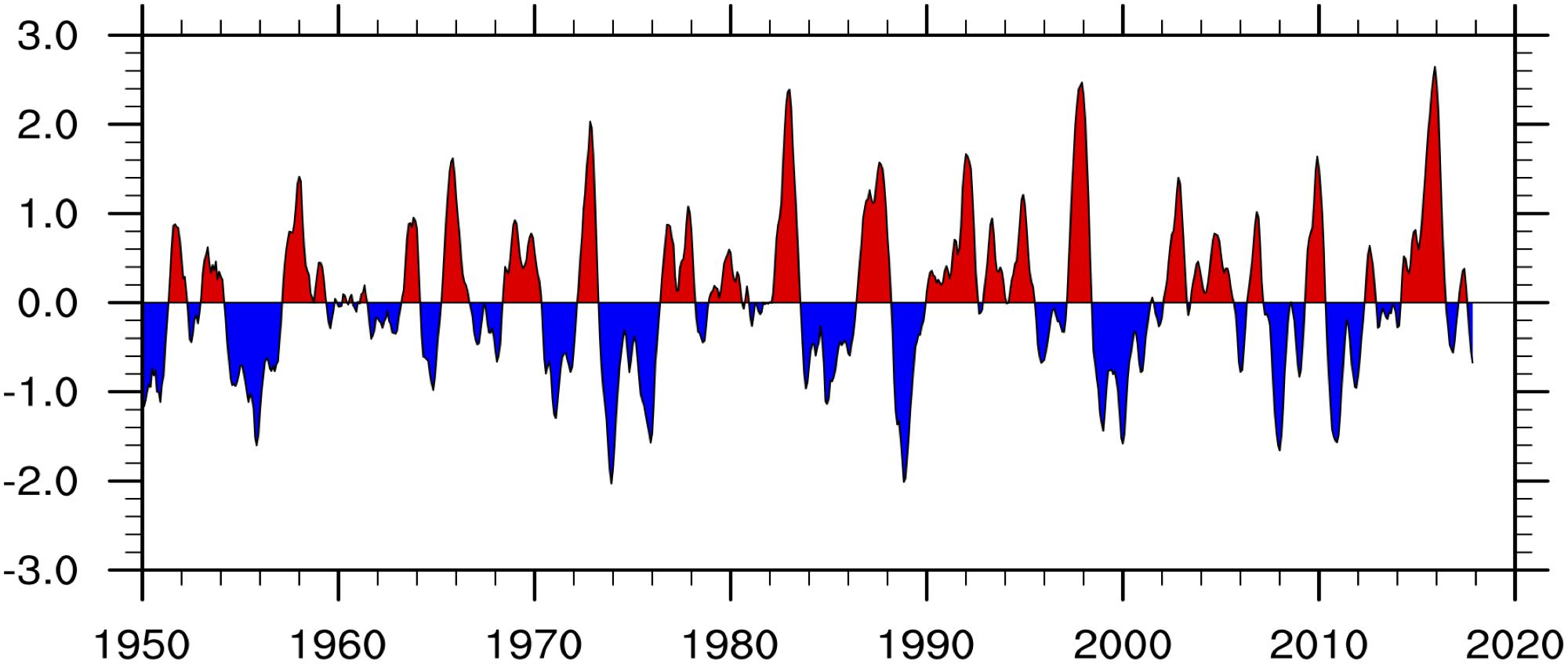
Figure 1. The running 3-month mean SST anomaly for the Niño 3.4 region from 1950 to 2017 with the 1950–2000 as the base period. Unit of SST anomaly is degree Celsius.

Meteorology Reanalysis Data

The NCEP/NCAR reanalysis I data are employed in this study. This reanalysis data is produced using a state-of-the-art analysis/forecast system that performs data assimilation using past observational data from 1948 to the present. The data span from 1948 to present at the 2.5° × 2.5° latitude-longitude resolution with 17 vertical levels (Kalnay et al., 1996). To investigate the relation between climate variables and ENSO, we use NCEP/NCAR monthly mean surface air temperature, SLP, and wind data for any identification of extreme heat or cold events, anomalies in large-scale atmospheric circulation, etc.

Precipitation Data

For flooding and drought extreme events, we use the Global Precipitation Climatology Project (GPCP) version 2.3 precipitation data from 1979 to the present at the 2.5° × 2.5° latitude-longitude resolution (Adler et al., 2016). The GPCP monthly product provides a consistent analysis of global precipitation from an integration of various satellite datasets over land and ocean, and a gauge analysis over land. Observational data from rain gauge stations, satellite, and sounding observations are merged to estimate monthly rainfall.

Methods and Model

In this study, we use two statistic methods (Granger causality method and Maximum lag correlation) and a global climate model (Community Atmospheric Model) to investigate the global impacts of ENSO on the climate variables.

Granger Causality Method

Granger causality could be calculated using different approaches such as vector autoregressive model (VAR), Graphical Lasso and SIN methods (Arnold et al., 2007). In this study, we use the VAR to determine the causality relation between ENSO and climate variables. The VAR includes two regressions: a regression function on predicting y based on its lagged values [Eq. (1)] and another regression predicting y based on lagged values of x and lagged value of y [Eq. (2)]. In [Eq. (2)], if no lagged values of x are retained in regression (i.e., all the coefficients of the terms are 0), we can conclude that y is not Granger caused by x.

$$y(t)=c_0+c_1\times y(t-1)+\mathrm{\cdots }+c_k\times y(t-k)+{\mathrm{\epsilon }}_t(1)$$

$$y(t)=a_0+a_1\times y(t-1)+\mathrm{\cdots }+a_k\times y(t-k)+b_l\times x(t-l)+\mathrm{\cdots }+b_n\times x(t-n)+{\mathrm{\epsilon }}_t(2)$$

Vector autoregressive model

An autoregressive (AR) model is usually used to measure the dependency of a variable on its own previous values.

Using AR(s) to denote an autoregressive model of order s, then the AR(s) on a series x(t) is defined as:

$$x\left(t\right)={\mathrm{\varnothing }}_0+{\mathrm{\varnothing }}_1\times x(t-1)+{\mathrm{\varnothing }}_2\times x(t-2)+\mathrm{\cdots }+{\mathrm{\varnothing }}_s\times x(t-s)+{\mathrm{\epsilon }}_t(3)$$

The vector autoregressive model is a particular case of the autoregressive model: VAR is used when we have more than one variable. Therefore, we will have the autoregressive model [Eq. (3)] on a vector. Given two time series x and y, VAR(p) on x and y is defined as

$$\left(\begin{array}{c}\hfill x(t)\hfill \\ \hfill y(t)\hfill \end{array}\right)=\left(\begin{array}{c}\hfill d_1\hfill \\ \hfill d_2\hfill \end{array}\right)+\left(\begin{array}{cc}\hfill d_{11}^1\hfill & \hfill d_{12}^1\hfill \\ \hfill d_{21}^1\hfill & \hfill d_{22}^1\hfill \end{array}\right)\times \left(\begin{array}{c}\hfill x(t-1)\hfill \\ \hfill y(t-1)\hfill \end{array}\right)+\mathrm{\cdots }+\left(\begin{array}{cc}\hfill d_{11}^p\hfill & \hfill d_{12}^p\hfill \\ \hfill d_{21}^p\hfill & \hfill d_{22}^p\hfill \end{array}\right)\times \left(\begin{array}{c}\hfill x\left(t-p\right)\hfill \\ \hfill y\left(t-p\right)\hfill \end{array}\right)+\left(\begin{array}{c}\hfill {\mathrm{\epsilon }}_{t1}\hfill \\ \hfill {\mathrm{\epsilon }}_{t2}\hfill \end{array}\right)(4)$$

The VAR can be applied to test the Granger causality of x and y: if at least one of the elements $d_{21}^i,i=1\mathrm{\cdots }p$ in [Eq. (4)] are non-zero, then y is Granger caused by x.

Implementation of the vector autoregressive model

In this study, we use the VAR package in Python to implement the vector autoregressive model. The lag order p is selected by an information criteria-based order selection. We choose the maximum number of lags to be 12 since there are 12 months per year. Then, the Schwarz’s criterion (Bayesian information criterion) (Kass and Wasserman, 1995) is used to select the “optimal” lag based on the data. Therefore, for different data set, the p value varies. The F-test is used to check the statistical significance. When we test the Granger causality of x and y, the null hypothesis is: y is not Granger caused by x (this is equivalent to all of the coefficients of x in the regression relation are 0). The F-test will give us two values: test statistic and critical value. The test statistic is also called F-statistic, giving by:

$$f=\frac{(R_u^2-R_r^2)/\mathrm{\gamma }}{R_u^2/(\mathrm{\theta }-\mathrm{\delta })}(5)$$

In [Eq. (5)], R²is the coefficient of determination which measures the strength of the linear relationship in the regression. $R_u^2$ is R²value from the unrestricted regression model [Eq. (2)]; $R_r^2$is the R² value from the restricted regression model [Eq. (1)]. γis the number of restrictions that depends on the lag order. θ is the number of observations and δ is the number of explanatory variables in the unrestricted model. In the F-test, this test statistic f will follow the F-distribution under the null hypothesis. The critical value can be obtained from the F distribution table.

Another way to use the F-test is to compare two values: the significance level α and the p-value p. The significance level is the probability of the study rejecting the null hypothesis; the p-value is the probability of obtaining a result at least as extreme, giving the null hypothesis were true. When we have p < α, we can conclude the result is statistically significant. In most cases, we choose the significance level to be 0.05. Therefore, if the p-value we get from the F-test is smaller than 0.05, we reject the null hypothesis which leads to the conclusion that y is Granger caused by x. In fact, when we have the test statistic is greater than the critical value, we will also have the p-value less than α. Therefore, the two approaches match with each other.

Maximum Lag Correlation

To compare with and to complement the Granger causality model, we also calculate the maximum lag correlation (i.e., cross correlation) between ENSO index and climate variables. It provides the maximum correlation coefficients between ENSO and climate variable and the corresponding lag time. The lag correlation coefficient between two series x(n) and y(n) is defined by Eq. (6), in which τ is the lag time, $\overline{\text{x}}$ and σ_x are the mean and standard deviation of the series x, respectively, and $\overline{\text{y}}$ and σ_y are the mean and standard deviation of the series y, respectively.

$$La{g}_{corr\left[\mathrm{\tau }\right]}=\frac{1}{n-\mathrm{\tau }}\sum _{k=1}^{n-\mathrm{\tau }}\left[\frac{x\left(k\right)-\overline{x}}{{\mathrm{\sigma }}_x}\times \frac{y\left(k+\mathrm{\tau }\right)-\overline{y}}{{\mathrm{\sigma }}_y}\right](6)$$

Global Climate Model

Based on physical hypothesis and sophisticated schemes, climate model is frequently used to find out the impact of a causing factor as effects on other parameters. For this study, series of sensitivity simulations are carried out with the global climate model forced by different simulated ENSO-like SST patterns to see the corresponding responses of atmospheric fields. The climate model we use in this study is the Community Atmospheric Model (version 5.3, CAM5.3) with the CAM5 standard parameterization schemes (Neale et al., 2010). The CAM5.3 uses the finite volume dynamical core at 1.9° latitude × 2.5° longitude resolution with 30 vertical levels and 1800-s time step. Simulations for three ENSO scenarios are carried out: (1) the control run forced with climatological SST; (2) the p2K run forced with climatological SST + 2°C at the Niño 3.4 region and climatological SST + 1°C at the central Pacific (10°S-10°N, 160°E-90°W); and (3) the n2K run forced with climatological SST – 2°C at the Niño 3.4 region and climatological SST – 1°C at the central Pacific (10°S-10°N and 160°E-90°W). The global distribution of climatological SST forcing used in the control run is shown in Figure 2A. The anomalies of the SST forcing used in the p2K run and n2K run with respect to the climatological SST are demonstrated in Figures 2B,C, respectively. In the light red (blue) region, the climatological SST is homogeneously increased (decreased) by 1°C, and in dark red (blue) region, the climatological SST is homogeneously increased (decreased) by 2°C to mimic strong positive (negative) ENSO scenarios (Figures 2B,C). The three simulations are run using MPI with 32 processors at UMBC Maya cluster¹. Each simulation is integrated for 36 months, and the last 24-month simulation outputs are used for analysis. We compare the changes in wind, SLP, cloud, precipitation and temperature fields from three simulations to our observation-based results using the statistical methods (i.e., Granger causality method and maximum lag correlation method) for consistency and discrepancy identifications.

FIGURE 2

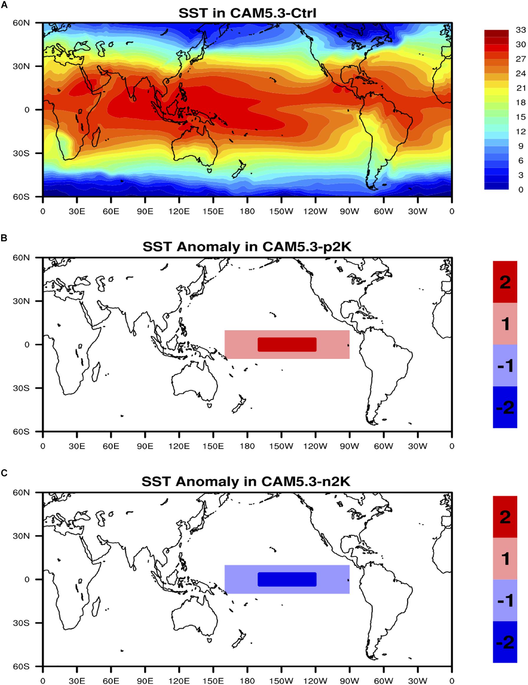
Figure 2. (A) Global distribution of annual mean SST used in the control run. (B) The SST anomaly used in the +2K run with respect to control run. (C) The SST anomaly used in the –2K run with respect to control run. Unit of SST is °C.

Results

ENSO vs. Surface Air Temperature (SAT)

First, we determine the cause-and-effect relation between ENSO and SAT on the global scale using the VAR method for Granger causality model. As the significant differences between Figures 3A,B are found, the changes in ENSO index clearly leads the changes in SAT in Figure 3A, but not vice versa in Figure 3B. This indicates SAT changes are Granger caused by ENSO, and ENSO is attributable for SAT anomalies, such as extreme heat or cold events, in remote regions such as South America, northwest North America, equatorial South Africa, and northern Australia. But ENSO variation is not caused by surface temperature over land. This result is consistent with the study of McGraw and Barnes (2018).

FIGURE 3

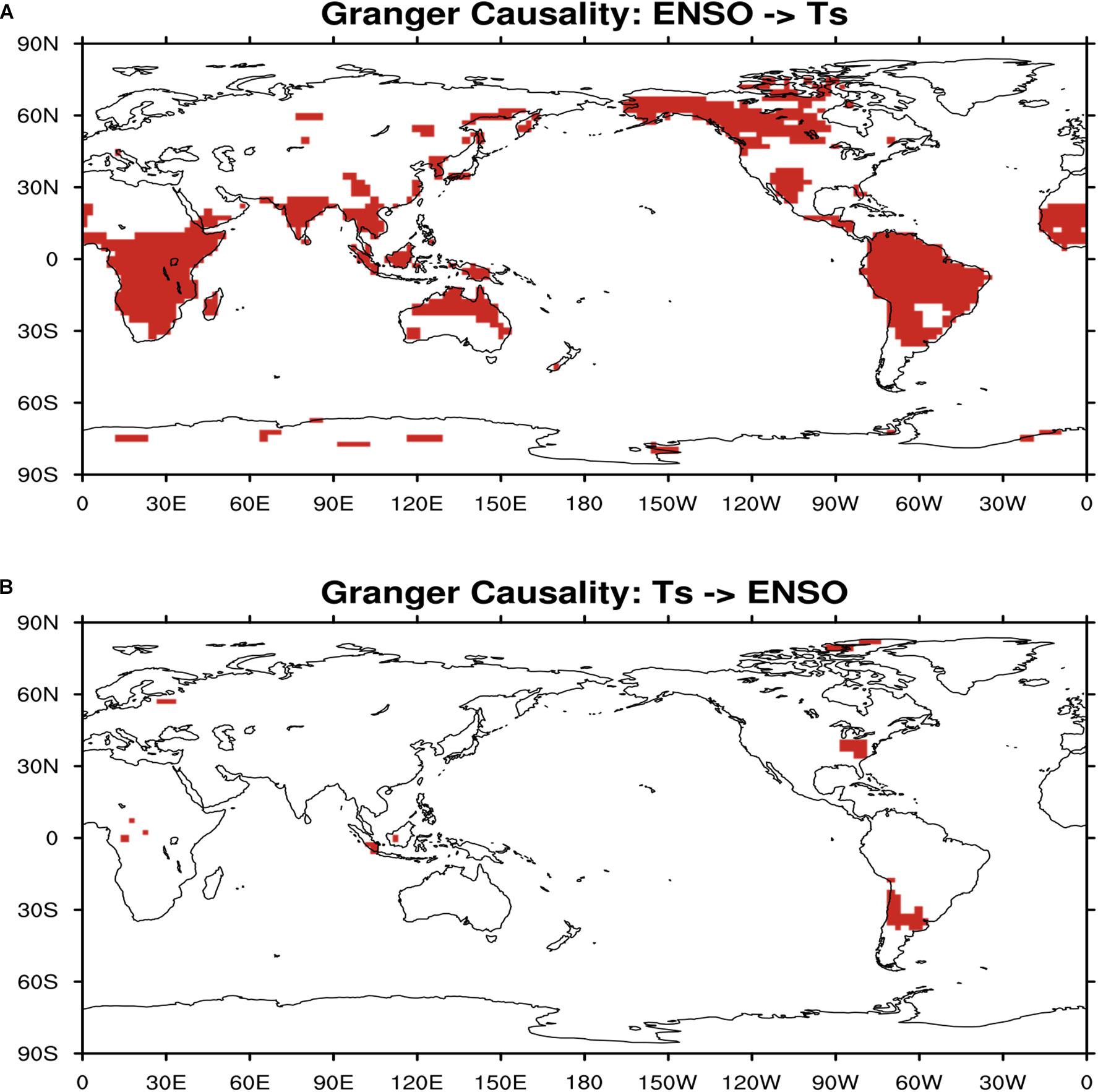
Figure 3. (A) Regions where surface air temperature is Granger caused by ENSO index (red shaded). (B) Regions where surface air temperature causes ENSO (red shaded).

The global distribution of the maximum lag correlation between ENSO index and surface temperature (Figure 4) shows that ENSO has strong positive relationship with surface temperature in South America and equatorial South Africa, which indicates that El Niño events (i.e., ENSO warm phase) are most likely accompanied with higher surface temperature over these lands. Results of the climate model sensitivity simulations (Figure 5) are consistent with the observational-based analyses. In the ENSO warm-phase events, there are positive anomalies in surface temperature over South America, northwest North America while in the ENSO cold-phase events there are negative anomalies in surface temperature over these regions.

FIGURE 4

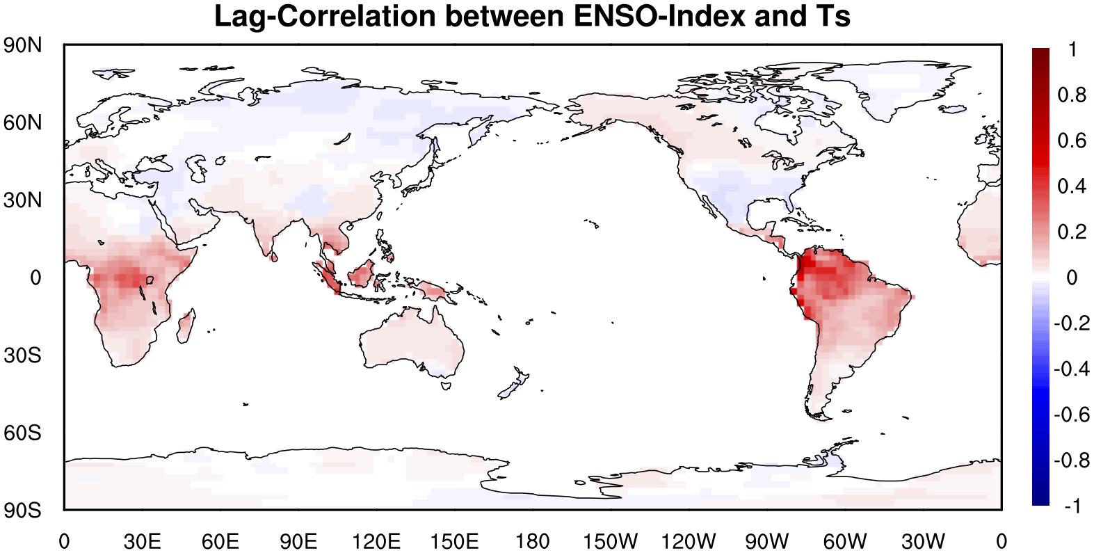
Figure 4. Maximum lag correlation between ENSO index and surface air temperature over land.

FIGURE 5

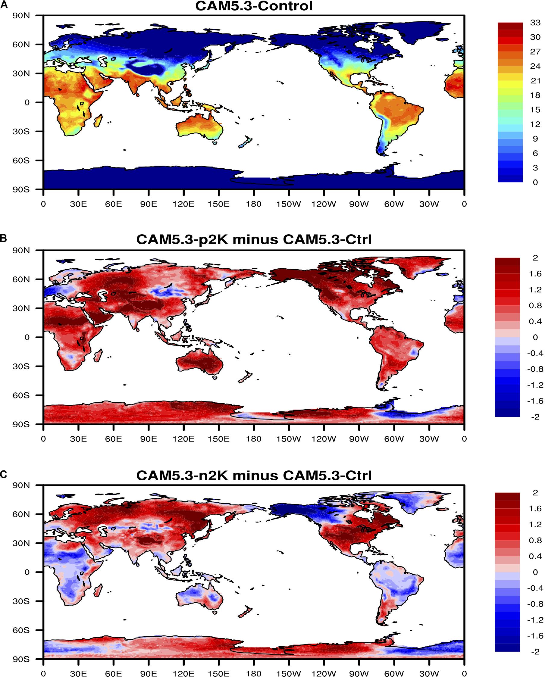
Figure 5. (A) Land surface air temperature in the CAM5 control run. (B) Anomalies of surface temperature in the CAM5 + 2K run with respect to the control run. (C) Anomalies of surface temperature in the CAM5-2K run with respect to the control run. Unit of temperature is °C.

ENSO vs. Sea Level Pressure (SLP)

In this study, we also investigate the causality relation between ENSO and SLP on the global scale for their spatio-temporal patterns. Comparing Figures 6A,B, we clearly observe that ENSO changes is leading the SLP changes and causing the SLP anomalies in the local and remote regions such as Pacific Ocean, Indian Ocean, and central Atlantic Ocean in Figure 6A; while ENSO changes are only caused by SLP over eastern Indian Ocean, tropical northern Pacific Ocean and southeastern Pacific Ocean, but at a much less significant level in Figure 6B. This is another indication that ENSO is the modulating factor in the cause-and-effect analysis with SLP, not vice versa.

FIGURE 6

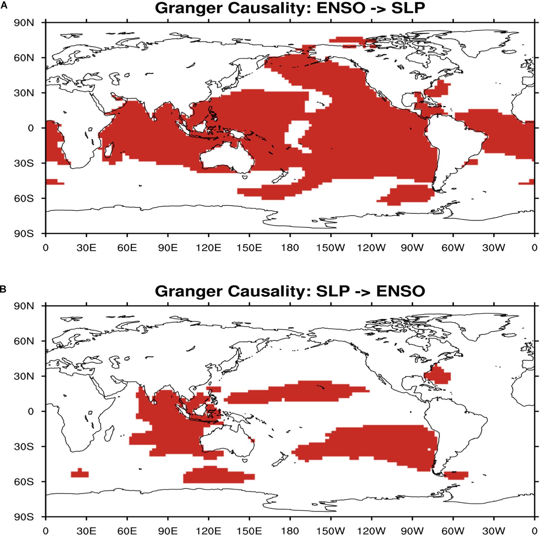
Figure 6. (A) Regions where sea level pressure is Granger caused by ENSO index (red shaded). (B) Regions where sea level pressure causes ENSO (red shaded).

The global distribution of the maximum lag correlation between ENSO index and SLP (Figure 7) shows that ENSO has strong positive relationship with SLP in the Tropical Western Pacific Ocean and strong negative relationship with SLP in the Eastern Pacific Ocean, which implies that El Niño events (i.e., ENSO warm phase) are most likely accompanied with higher SLP over the Tropical Western Pacific Ocean and lower SLP over the Eastern Pacific Ocean. Results of the climate model sensitivity simulations (Figure 8) are consistent with the observational-based analyses. In the ENSO warm-phase events, there are negative anomalies in SLP over Eastern Pacific Ocean while in the ENSO cold-phase events there are positive anomalies in SLP over Eastern Pacific Ocean and negative anomalies in SLP over Tropical Western Pacific Ocean and Indian Ocean. Such consistency between observational evidence and model simulations give us more confidence that ENSO is modulating SLP remotely as the causing factor, thus the spatio-temporal patterns with ENSO leading SLP can be more readily explained as ENSO causing anomalies in SLP over other parts of the world.

FIGURE 7

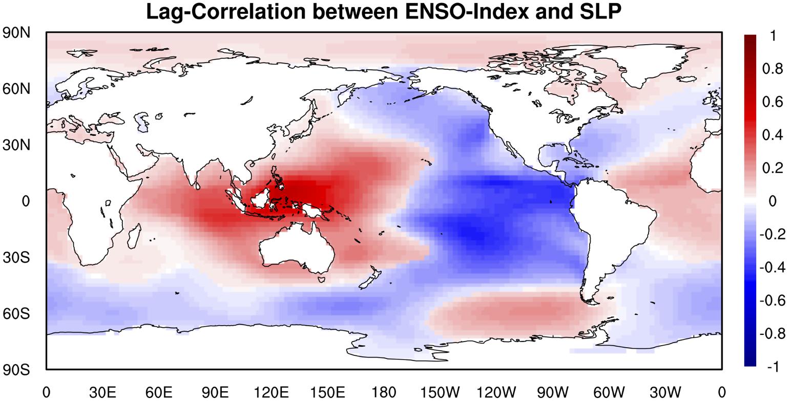
Figure 7. Maximum lag correlation between ENSO index and sea level pressure.

FIGURE 8

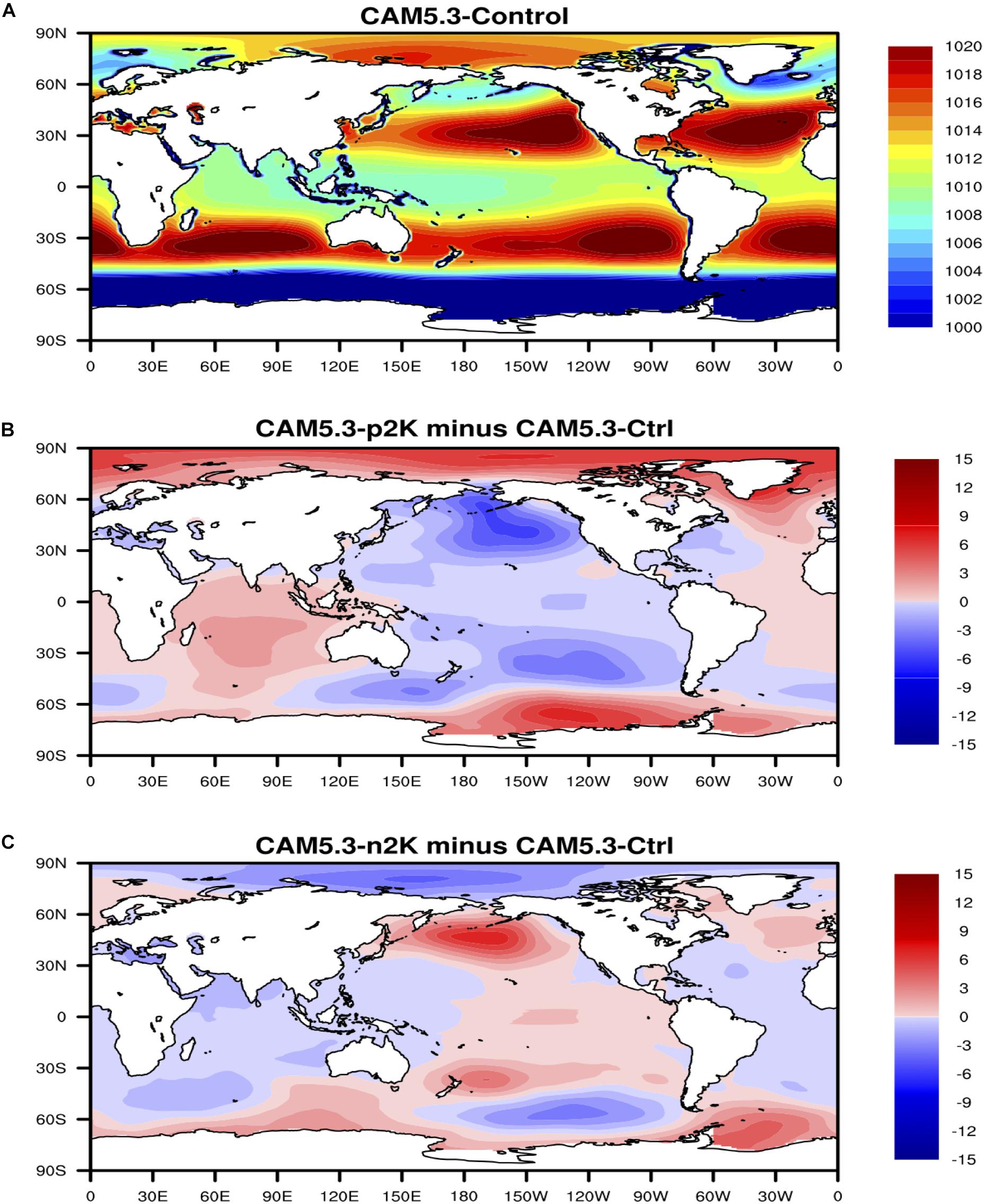
Figure 8. (A) Sea level pressure in the CAM5 control run. (B) Anomalies of SLP in the CAM5 + 2K run with respect to the control run. (C) Anomalies of SLP in the CAM5-2K run with respect to the control run. Unit of SLP is hPa.

ENSO vs. Precipitation

To explore the relationship between extreme flooding and drought with ENSO, we analyze the causality relation between ENSO and surface precipitation on the global scale. As the comparison between Figures 9A,B shows, the ENSO changes are leading the changes in surface precipitation anomalies in many regions such as tropical Ocean and tropical land, with significant Granger causality correlation over broad area in Figure 9A, but not vice versa in Figure 9B.

FIGURE 9

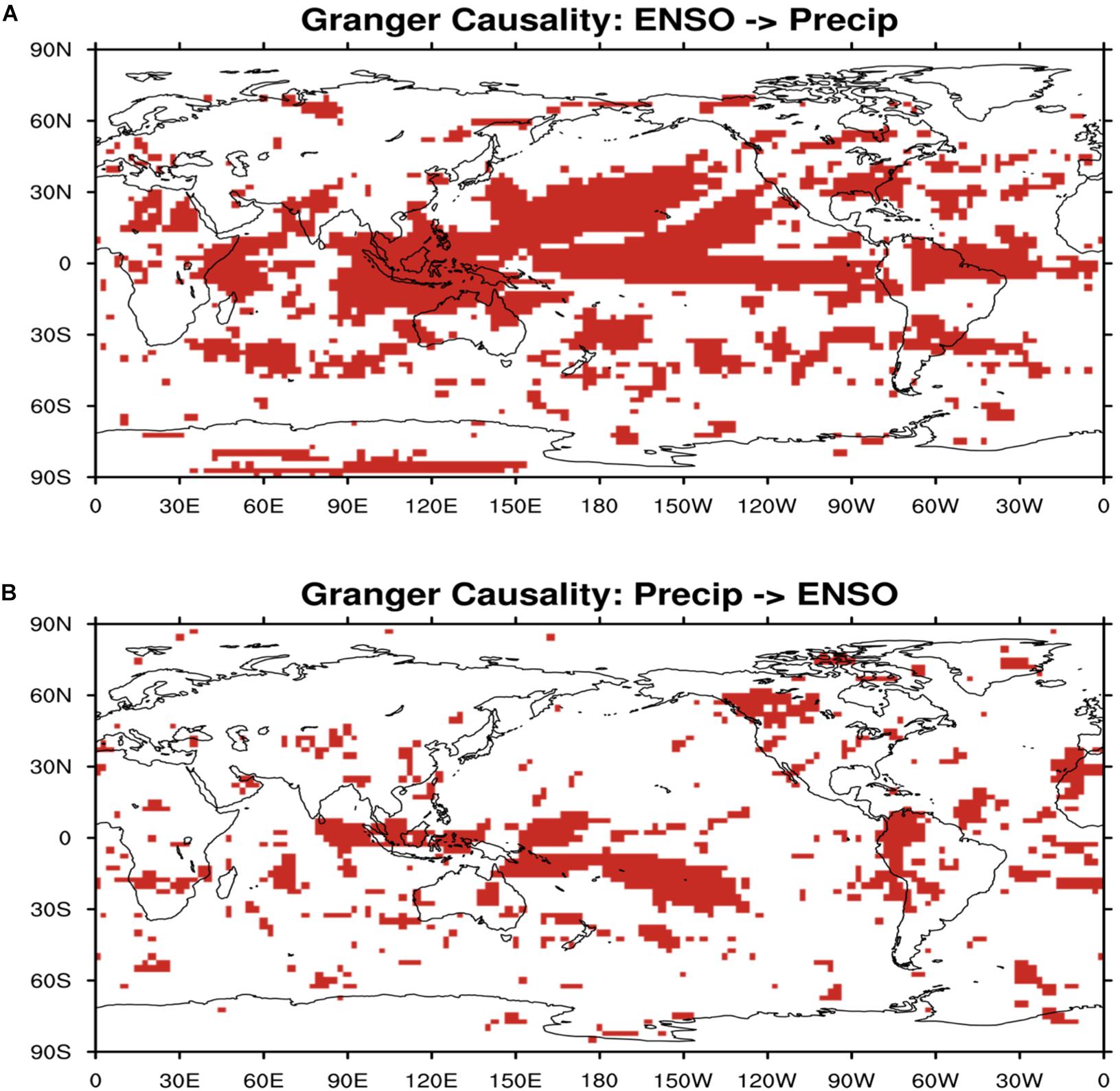
Figure 9. (A) Regions where surface precipitation is granger caused by ENSO index (red shaded). (B) Regions where surface precipitation causes ENSO (red shaded).

The global distribution of the maximum lag correlation between ENSO index and surface precipitation (Figure 10) shows that ENSO has strong negative relationship with surface precipitation in Tropical Western Pacific and tropical South American, indicating ENSO’s remote impact on extreme drought events. Figure 10 also shows ENSO has strong positive relationship with surface precipitation in Tropical Central and Eastern Pacific, which means ENSO may potentially result in extreme flooding events over these regions. Similarly, the climate model sensitivity simulations (Figure 11) indicate that in the ENSO warm-phase events, there are positive anomalies (floods) in surface precipitation over Tropical Central and Eastern Pacific, and negative anomalies (droughts) in surface precipitation over Tropical Western Pacific, consistent to what we found from the observations. The patterns of precipitation anomalies in the ENSO cold-phase events are clearly different from those in the ENSO warm-phase events.

FIGURE 10

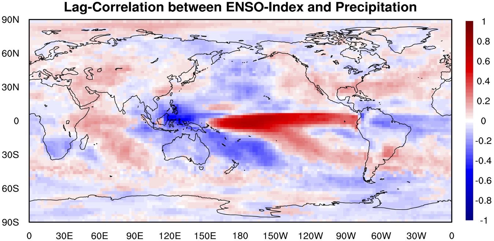
Figure 10. Maximum lag correlation between ENSO index and precipitation.

FIGURE 11

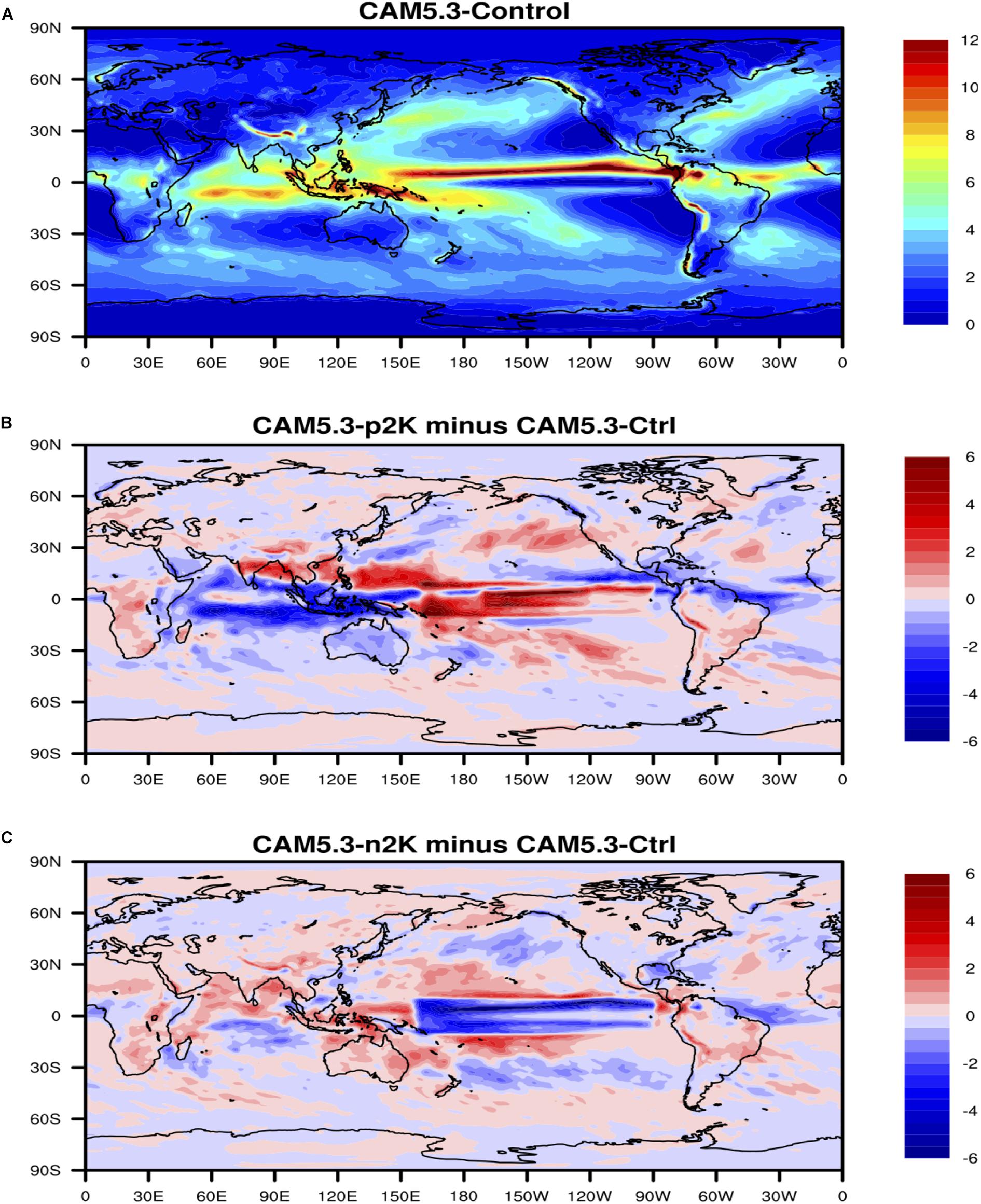
Figure 11. (A) Surface precipitation in the CAM5 control run. (B) Anomalies of precipitation in the CAM5 + 2K run with respect to the control run. (C) Anomalies of precipitation in the CAM5-2K run with respect to the control run. Unit of precipitation is mm/day.

ENSO vs. Circulation

Occurrence of different climate events strongly depends on the large-scale atmospheric circulation. Mid-tropospheric (500 hPa) vertical pressure velocity is widely used as a proxy for the large-scale tropical circulation (Bony et al., 2004). Lastly for this study, we explored the causality relation between ENSO and 500 hPa vertical pressure velocity using the same VAR method for Granger causality. As shown in Figures 12A vs. B, ENSO seems to cause 500 hPa vertical velocity anomalies significantly over very broad areas in most Tropical Pacific Ocean in Figure 12A, but not vice versa in Figure 12B.

FIGURE 12

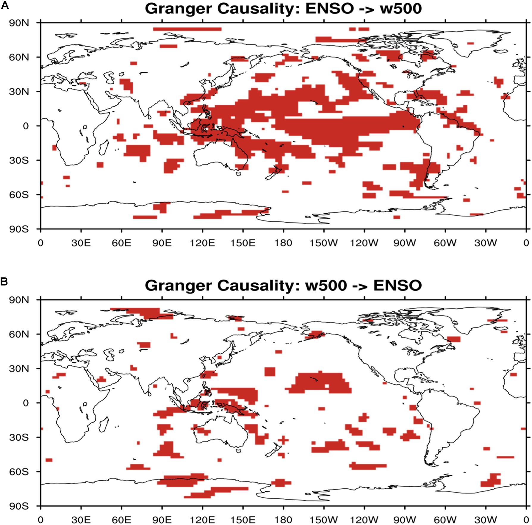
Figure 12. (A) Regions where 500 hPa vertical velocity is granger caused by ENSO index (red shaded). (B) Regions where 500 hPa vertical velocity causes ENSO (red shaded).

The global distribution of the maximum lag correlation between ENSO index and 500 hPa vertical velocity (Figure 13) is almost same as that for surface precipitation (Figure 10) but with opposite signs, i.e., ENSO has strong positive relationship with 500 hPa vertical velocity in Tropical Western Pacific and tropical South American, an indication of ENSO warm phase suppresses deep convection and cold phase invigorates deep convection instead. At the same time, ENSO has strong negative relationship with vertical wind over Tropical Central and Eastern Pacific, which means ENSO warm phase potentially invigorates deep convection over these areas and cold phase suppresses deep convection instead. Results of the climate model sensitivity simulations (Figure 14) are considerably similar to those of the observational-based analyses in Figures 12, 13. In the ENSO warm-phase events, there are positive anomalies in 500 hPa vertical velocity over the Tropical Western Pacific and negative anomalies in 500 hPa vertical velocity over the Tropical Central and Eastern Pacific. Putting the results in the context of Pacific atmospheric circulation, ENSO warm phase weakens Pacific walker circulation but ENSO cold phase enhances Pacific walker circulation, consistent to what is reported in Yeh et al. (2017).

FIGURE 13

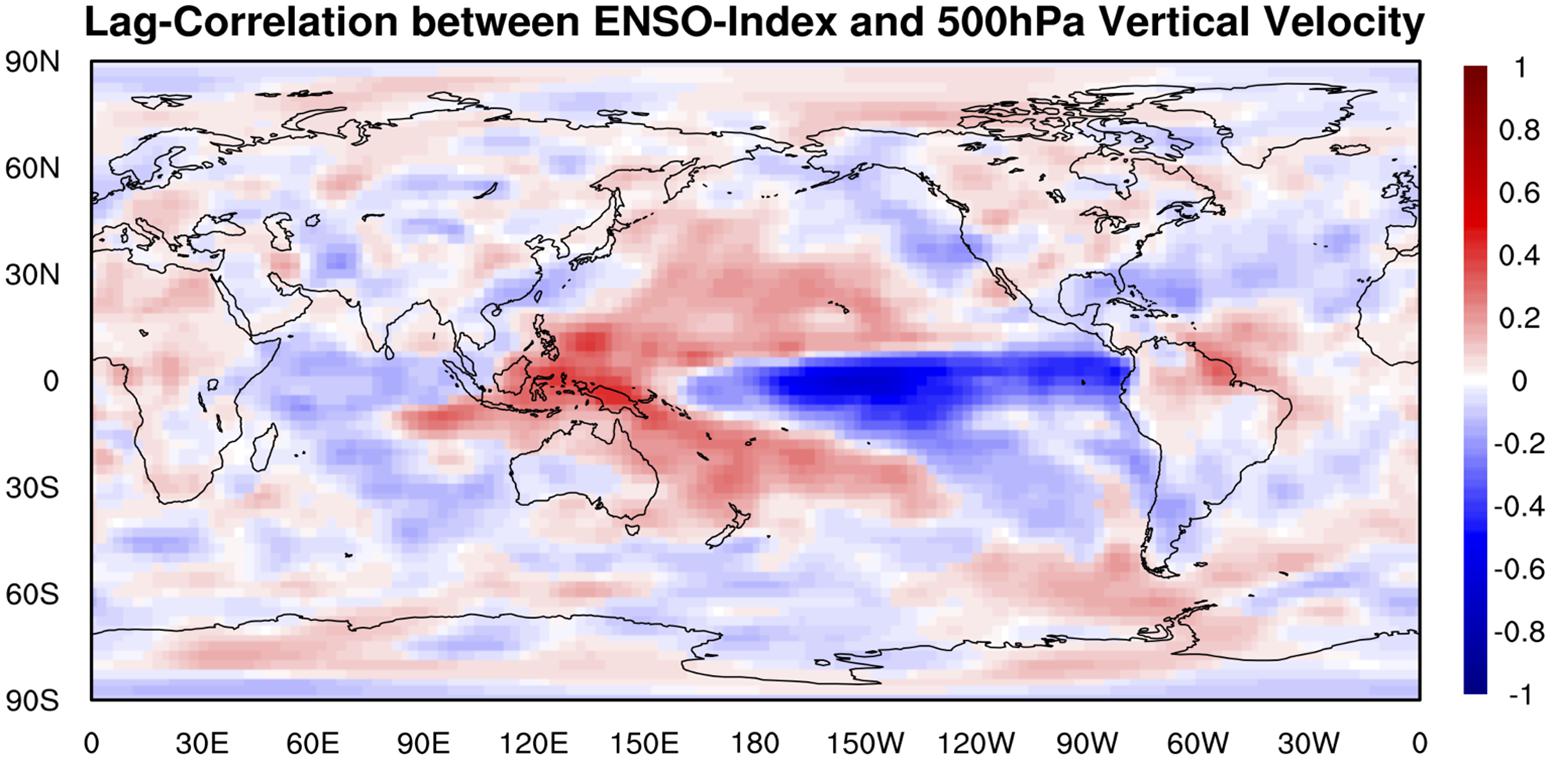
Figure 13. Maximum lag correlation between ENSO index and 500 hPa vertical velocity.

FIGURE 14

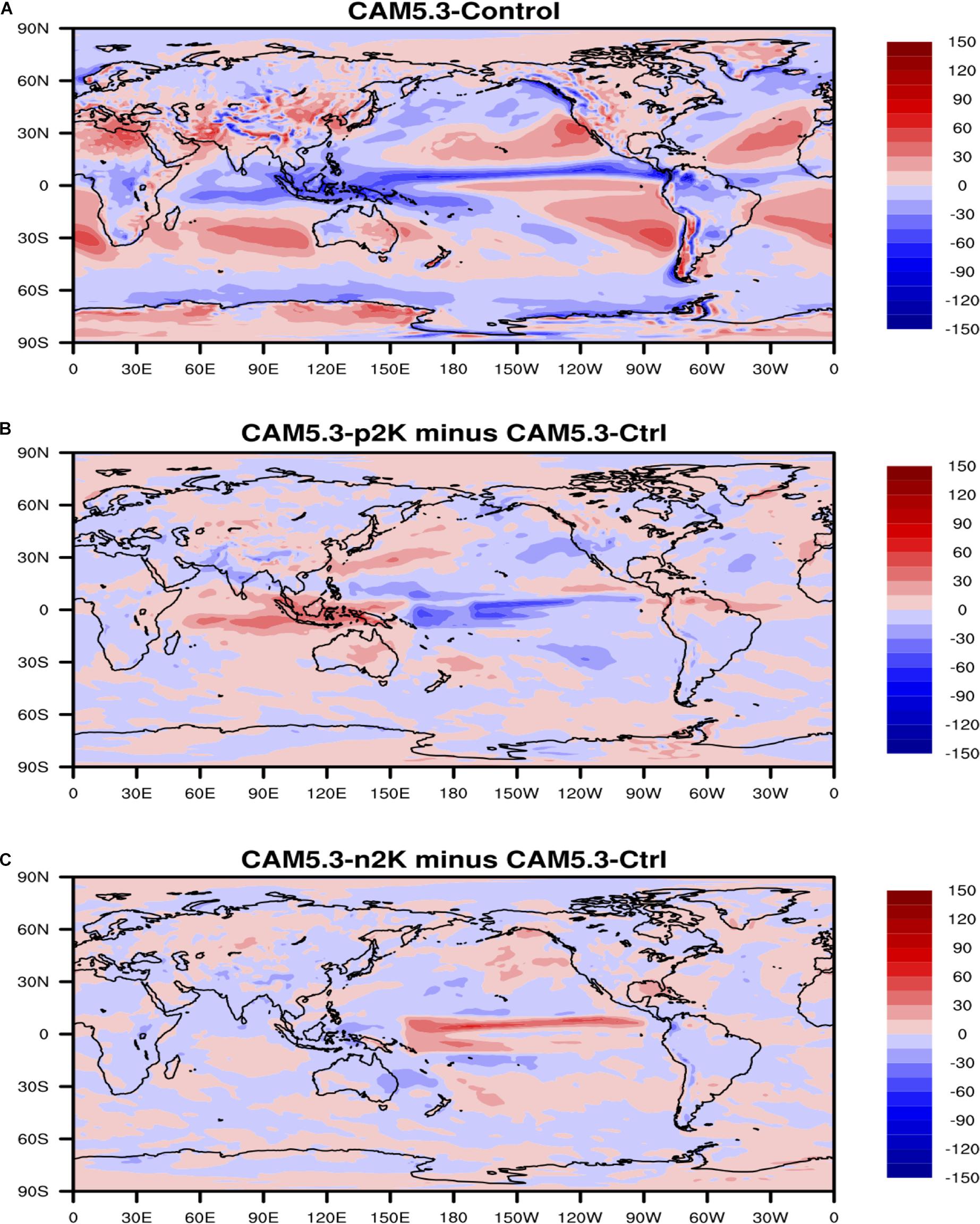
Figure 14. (A) 500 hPa vertical velocity in the CAM5 control run. (B) Anomalies of 500 hPa vertical velocity in the CAM5 + 2K run with respect to the control run. (C) Anomalies of 500 hPa vertical velocity in the CAM5-2K run with respect to the control run. Unit of 500 hPa vertical velocity is hPa/day.

Discussion

In this study, we use statistical methods, namely the VAR method for Granger causality model, and global climate model simulations to investigate ENSO causality as one of the modulating climate factors that cause the anomalies in surface air temperature, precipitation, surface pressure, and vertical wind over remote regions through teleconnection with lagged temporal variability. We analyzed different observational data, reanalysis data, and model data to comprehensively investigate the global impacts of ENSO. The Granger causality analysis was able to clearly show ENSO as a cause instead of an effect to influence the remote climate variables and thus cause extreme weather events such as flooding, drought, extreme heat, and cold, etc. Our model simulations using the CAM5.3 also successfully simulated ENSO’s remote impacts on other weather variables, consistent to the findings from observational evidence. Besides, all the source codes used in this study can be found on Github².

For future work, we will compare the Granger causality on multiple variables for intercomparison, and we will add analysis on the impact of ENSO on clouds and aerosol using NASA satellite remote sensing data. We plan to use the Granger causality methods to predict climate variations and other interesting economic factors, such as crop yield and wheat stock price, under different ENSO backgrounds. At the same time, we plan to explore more efficient use of high performance parallel computing in the studies that use much broader big data of satellite observations with higher spatial and temporal resolutions.

Data Availability

The datasets analyzed for this study can be found in HadISST at https://www.metoffice.gov.uk/hadobs/hadisst/, NCEP/NCAR at https://www.esrl.noaa.gov/psd/data/gridded/data.ncep.reanalysis.html, and Global Precipitation Climate Project Precipitation (GPCP) at https://www.esrl.noaa.gov/psd/data/gridded/data.gpcp.html. Besides, all the source codes used in this study can be found on https://github.com/big-data-lab-umbc/cybertraining/tree/master/year-1-projects/team-4.

Author Contributions

HS, JT, JH, and PG worked on the implementation and experiment. All authors worked on the research topic, approach, plan, and approved the manuscript.

Conflict of Interest Statement

JH was employed by the company Science Systems and Applications, Inc.

The remaining authors declare that the research was conducted in the absence of any commercial or financial relationships that could be construed as a potential conflict of interest.

Funding

This work was supported by the grant CyberTraining: DSE: Cross-Training of Researchers in Computing, Applied Mathematics, and Atmospheric Sciences using Advanced Cyberin-frastructure Resources from the National Science Foundation (Grant No. OAC–1730250). The hardware in the UMBC High Performance Computing Facility (HPCF) was supported by the U.S. National Science Foundation through the MRI program (Grant Nos. CNS–0821258, CNS–1228778, and OAC–1726023) and the SCREMS program (Grant No. DMS–0821311), with additional substantial support from the University of Maryland, Baltimore County (UMBC). See hpcf.umbc.edu for more information on HPCF and the projects using its resources.

Footnotes

1. ^ http://hpcf.umbc.edu/
2. ^ https://github.com/big-data-lab-umbc/cybertraining/tree/master/year-1-projects/team-4

References

Adler, R., Sapiano, M., Huffman, G. J., Bolvin, D., Wang, J.-J., and Nelkin, E. (2016). New global precipitation climatology project monthly analysis product corrects satellite data drifts. GEWEX News 26, 7–9.

Google Scholar

Arnold, A., Liu, Y., and Abe, N. (2007). “Temporal causal modeling with graphical granger methods,” in Proceedings of the 13th ACM SIGKDD International Conference on Knowledge Discovery and Data Mining, (San Jose, CA), 66–75.

Google Scholar

Boening, C., Willis, J. K., Landerer, F. W., Nerem, R. S., and Fasullo, J. (2012). The 2011 La Niña: so strong, the oceans fell. Geophys. Res. Lett. 39:L19602. doi: 10.1029/2012GL053055

CrossRef Full Text | Google Scholar

Bony, S., Dufresne, J.-L., LeTreut, H., Morcrette, J.-J., and Senior, C. (2004). On dynamic and thermodynamic components of cloud changes. Clim. Dyn. 22, 71–86. doi: 10.1007/s00382-003-0369-6

CrossRef Full Text | Google Scholar

Cazenave, A., Henry, O., Munier, S., Delcroix, T., Gordon, A. L., Meyssignac, B., et al. (2012). Estimating ENSO influence on the global mean sea level 1993-2010. Mar. Geod. 35, 82–97. doi: 10.1080/01490419.2012.718209

CrossRef Full Text | Google Scholar

Chen, Y., Randerson, J. T., Morton, D. C., DeFries, R. S., Collatz, G. J., and Kasibhatla, P. S. (2011). Forecasting fire season severity in south America using sea surface temperature anomalies. Science 334, 787–791. doi: 10.1126/science.1209472

PubMed Abstract | CrossRef Full Text | Google Scholar

Elsner, J. (2007). Granger causality and atlantic hurricanes. Tellus 59A, 476–485. doi: 10.1111/j.1600-0870.2007.00244.x

CrossRef Full Text | Google Scholar

García-Serrano, J., Frankignoul, C., Gastineau, G., and de la Cámara, A. (2015). On the predictability of the winter Euro-Atlantic climate: lagged influence of autumn Arctic sea ice. Clim. J. 28, 5195–5216. doi: 10.1175/jcli-d-14-00472.1

CrossRef Full Text | Google Scholar

Granger, C. (1969). Investigating causal relations by econometric models and cross-spectral methods. Econometrica 37, 424–438.

Google Scholar

Gross, R. S., Marcus, S. L., and Dickey, J. O. (2002). “Modulation of the seasonal cycle in length-of-day and atmospheric angular momentum,” in Proceedings of IAG Symposia, 2001: Vistas for Geodesy in the New Millennium, Vol. 125, (Berlin: Springer), 457–462. doi: 10.1007/978-3-662-04709-5_76

CrossRef Full Text | Google Scholar

Gross, R. S., Marcus, S. L., Eubanks, T. M., Dickey, J. O., and Keppenne, C. L. (1996). Detection of an ENSO signal in seasonal length-of-day variations. Geophys. Res. Lett. 23, 3373–3376. doi: 10.1029/96GL03260

CrossRef Full Text | Google Scholar

Gu, G., and Adler, R. F. (2011). Precipitation and temperature variations on the interannual time scale: assessing the impact of ENSO and volcanic eruptions. J. Clim. 24, 2258–2270. doi: 10.1175/2010jcli3727.1

CrossRef Full Text | Google Scholar

Haddad, M., and Bonaduce, A. (2017). Interannual variations in length of day with respect to El Niño - Southern Oscillation’s impact (1962–2015). Arabian J. Geosci. 10:255. doi: 10.1007/s12517-017-3049-2

CrossRef Full Text | Google Scholar

Haddad, M., Taibi, H., and Mohammed Arezki, S. M. (2013). On the recent global mean sea level changes: trend extraction and El Nino’s impact. C. R. Geosci. 345, 167–175. doi: 10.1016/j.crte.2013.03.002

CrossRef Full Text | Google Scholar

Höpfner, J. (1999). “Interannual variations in length of Day and atmospheric angular momentum with respect to ENSO cycles,” in Paper Presented at the 22nd General Assembly International Union of Geodesy and Geophysics, (Birmingham).

Google Scholar

Kalnay, E., Kanamitsu, M., Kistler, R., Collins, W., Deaven, D., and Gandin, L. (1996). The NCEP/NCAR 40-year reanalysis project. Bull. Amer. Meteor. Soc. 77, 437–470.

Google Scholar

Kass, R. E., and Wasserman, L. (1995). A reference bayesian test for nested hypotheses and its relationship to the schwarz criterion. J. Am. Stat. Assoc. 90, 928–934. doi: 10.1080/01621459.1995.10476592

CrossRef Full Text | Google Scholar

Kretschmer, M., Coumou, D., Donges, J. F., and Runge, J. (2016). Using causal effect networks to analyze different Arctic drivers of midlatitude winter circulation. J. Clim. 29, 4069–4081. doi: 10.1175/jcli-d-15-0654.1

CrossRef Full Text | Google Scholar

Kumar, A., Zhang, L., and Wang, W. (2012). Sea surface temperature - precipitation relationship in different reanalyses. Mon. Weather Rev. 141, 1118–1123. doi: 10.1175/mwr-d-12-00214.1

CrossRef Full Text | Google Scholar

Lozano, A. C., Naoki, A., Liu, Y., and Rosset, S. (2009). “Grouped graphical granger modeling methods for temporal causal modeling,” in Proceedings of the 15th ACM SIGKDD International Conference on Knowledge Discovery and Data Mining, (New York, NY: Association for Computing Machinery), 577–586.

Google Scholar

McGraw, M., and Barnes, E. A. (2018). Memory matters: a case for granger causality in climate variability studies. J. Clim. 31, 3289–3300. doi: 10.1175/jcli-d-17-0334.1

CrossRef Full Text | Google Scholar

Mokhov, I., Smirnow, D., Nakonechny, P., Kozlenko, S., Selezn, E., and Kurths, J. (2011). Alternating mutual influence of El-Niño/Southern Oscillation and Indian monsoon. Geophys. Res. Lett. 38:L00F04.

Google Scholar

Neale, R. B., Chen, C.-C., Gettelman, A., Lauritzen, P. H., Park, S., and Williamson, D. L. (2010). Description of the NCAR Community Atmosphere Model (CAM 5.0). Tech. Rep. TN–486+STR. Boulder, CO, 268.

Google Scholar

Ngo-Duc, T., Laval, K., Polcher, J., and Cazenave, A. (2005). Contribution of continental water to sea level variations during the 1997-1998 El Niño-Southern Oscillation event: comparison between atmospheric model intercomparison project simulations and TOPEX/Poseidon satellite data. J. Geophys. Res. 110:D09103. doi: 10.1029/2004JD004940

CrossRef Full Text | Google Scholar

Rayner, N. A., Parker, D. E., Horton, E. B., Folland, C. K., Alexander, L. V., Rowell, D. P., et al. (2003). Global analyses of sea surface temperature, sea ice, and night marine air temperature since the late nineteenth century. J. Geophys. Res. 108:4407.

Google Scholar

Runge, J., Petoukhov, V., and Kurths, J. (2014). Quantifying the strength and delay of climatic interactions: the ambiguities of cross correlation and a novel measure based on graphical models. J. Clim. 27, 720–739. doi: 10.1175/jcli-d-13-00159.1

CrossRef Full Text | Google Scholar

Song, H., Wang, J., Tian, J., Huang, J., and Zhang, Z. (2018). “Spatio-temporal climate data causality analytics – an analysis of ENSO’s global impacts,” in Proceedings of the 8th International Workshop on Climate Informatics, 45–48.

Google Scholar

Tabari, H., and Willems, P. (2018). Lagged influence of atlantic and pacific climate patterns on European extreme precipitation. Sci. Rep. 8:5748. doi: 10.1038/s41598-018-24069-9

PubMed Abstract | CrossRef Full Text | Google Scholar

Yeh, S.-W., Cai, W., Min, S.-K., McPhaden, M. J., Dommenget, D., Dewitte, B., et al. (2017). ENSO atmospheric teleconnections and their response to greenhouse gas forcing. Rev. Geophys. 56, 185–206. doi: 10.1002/2017RG000568

PubMed Abstract | CrossRef Full Text | Google Scholar