 Shiru Tan1,2
 Jingjing Zhang2,3
 Hongliang Li2*
 Lin Sun2
 Zezhou Wu2
 Martin G. Wiesner2
 Hao Zheng1
 Jianfang Chen2,4*
- 1Ocean College, Zhejiang University, Zhoushan, China
- 2Key Laboratory of Marine Ecosystem Dynamics, Second Institute of Oceanography, Ministry of Natural Resources, Hangzhou, China
- 3Southern Marine Science and Engineering Guangdong Laboratory (Zhuhai), Zhuhai, China
- 4State Key Laboratory of Satellite Ocean Environment Dynamics, Second Institute of Oceanography, Ministry of Natural Resources, Hangzhou, China
Based on a time-series sediment trap observation at a depth of 1,003-m in the northern South China Sea from 2014 to 2015, we used sinking particle flux combined with remote sensing-derived environmental data to infer the mechanisms of the biological carbon pump. Total particle flux, particulate organic carbon, CaCO3, and lithogenic (inorganic) fluxes peaked in winter and autumn but showed minima in summer, ranging from 59.7 to 413.2 mg m–2 d–1, 2.1 to 18.2 mg m–2 d–1, 32.9 to 197.9 mg m–2 d–1, and 12.0 to 73.6 mg m–2 d–1, respectively. Similarly, opal flux varied from 6.9 to 109.6 mg m–2 d–1, with a prominent peak in winter and minimum in summer. However, a secondary maximum of opal in autumn was barely noticeable compared with other components. A deeper mixed-layer depth related to the northeast monsoon and surface cooling, overlapping with the effect of cyclonic eddies, is responsible for strong winter fluxes. When an anticyclonic eddy suppresses the subsurface nutrient supply, primary production and subsequent export flux in summer were reduced substantially. With respect to maximum lithogenic and CaCO3 fluxes in autumn, a large aerosol optical depth suggests scavenging and mineral ballast effects as potential causes. This study highlights the importance of intra-seasonal physical processes (e.g., mesoscale eddies and aerosol deposition) to the deep particle flux in the South China Sea, as well as monsoonal transition.
Introduction
The overuse of fossil fuels by human activities and the destruction of the natural environment such as deforestation has increased the atmospheric concentration of CO2 from 280 ppm before the Industrial Revolution, to around 406 ppm today1. This has led to global warming and a rise in sea level. Among the most important factors driving global atmospheric concentration of CO2 and climate change during the glacial-interglacial period were biogeochemical processes in the ocean (Broecker, 1982; Sigman and Boyle, 2000). The key to the removal of atmospheric CO2 is the marine “biological pump” in which oceanic photosynthetic organisms take up inorganic matter as inorganic carbon and inorganic nutrients to synthesize particulate organic matter and export it to the deep sea (Volk and Hoffert, 1985).
Most of the settling particulate organic carbon (POC) in the deep ocean is composed of fine organic residues, including phytoplankton debris and zooplankton fecal pellets. In general, the export of organic matter from surface water is mainly controlled by net primary productivity (NPP) in the euphotic layer (Eppley and Peterson, 1979), particle sinking, and degradation rates (Francois et al., 2002). First, the NPP level is subjected to physical processes of different spatial and temporal scales that regulate the supply of nutrients to the overlying water, affecting the type and flux of subsequent carbon export (Nair et al., 1989; Archer and Maier-Reimer, 1994; Honjo et al., 1999). Next, biogenic (calcium carbonate, CaCO3 and biogenic silica, opal) and lithogenic (aluminosilicates for example) minerals in the ocean have an impact on the formation, sedimentation, and preservation of POC (Armstrong et al., 2002; Francois et al., 2002; Klaas and Archer, 2002; Passow et al., 2006). When a mineral aggregated with POC, it had a “ballasting effect” on the particle. On one hand, it can increase the density of the settling particles, thereby accelerating the sinking rate. In addition, the mineral can provide physical protection and reduce the microbial degradation of organic matter (Lee et al., 2009). On a global scale, this effect is most relevant to the flux of biogenic minerals, especially CaCO3 (Klaas and Archer, 2002; Barker et al., 2003), but in the marginal seas strongly affected by trade winds, monsoons and large rivers, like the Atlantic coastal regions, POC export is remarkably influenced by the ballast effect of lithogenic material from atmospheric deposition (Fischer and Karaka, 2009; Salter et al., 2010).
Located between the western Pacific warm pool and Qinghai–Tibet Plateau, the South China Sea (SCS) has an area of ∼3.5 × 10⁶ km2 and maximum water depth of ∼5,500 m. The sea receives intense solar radiation and there is high sea surface temperature (SST) year-round, resulting in a strong vertical stratification of the water. The SCS is a typical surface oligotrophic area with surface nitrate, phosphate and silicate concentration below 1, 0.1, and 5 μmol/L, respectively (Wong et al., 2002) and of weak productivity (Liu et al., 2002; Wong et al., 2007). Because of distinct land–sea thermal differences, the East Asian monsoon prevails over the SCS. Under the persistent influence of monsoonal winds, a large-scale cyclonic circulation gyre develops across the entire SCS during the winter (northeast) monsoon and an anticyclonic circulation gyre covering the southern half of the sea during the summer (southwest) monsoon (Shaw and Chao, 1994; Xue et al., 2004). Meanwhile, there is upwelling along the Sunda Shelf and off Luzon Island of the Philippines during winter and off the southeastern coasts of the Indochinese Peninsula during the summer monsoon (Liu et al., 2002; Xie et al., 2003). At present, the long-term record of total particulate flux (TPF), POC, CaCO3, and opal fluxes based on sediment traps in the northern SCS shows a distinct winter maximum pattern (Wiesner et al., 1996; Wong et al., 2007). The pronounced winter peak might be induced by the combined interaction of surface cooling and wind-induced mixing, which pumps eutrophic subsurface water to the euphotic layer and promotes primary production (Tseng et al., 2005). Findings from sediment trap samples in the SCS area have shown a strong winter signal in amino acid fluxes (Lahajnar et al., 2007), δ18O of planktonic foraminifera (Lin et al., 2004, 2011), mean δ15N values at various depths (Kao et al., 2012), nitrogen flux (Gaye et al., 2009), downward fluxes of coccoliths (Ran et al., 2015), and 210Pb flux which correlates with particulate fluxes positively (Chung et al., 2004). Besides the winter peak, the central SCS has a secondary maximum of downward carbon fluxes during the summer monsoon (Lahajnar et al., 2007). Notwithstanding a lack of consensus, the summer secondary maximum may be driven by the horizontal advection of nutrients and biogenic particles from the summer jet off Vietnam to the central basin (Chen and Wang, 2015).
Moreover, the monsoon transports numerous airborne particles from the Asian mainland (Duce and Tindale, 1991). Studies have revealed that atmospheric dust from the eastern Asian continent can be carried distances in excess of 1,000 km (Wang et al., 2011). Dust input not only acts as mineral ballast material but also transfers macronutrients and bio-available iron to oligotrophic surface water (Wong et al., 2007; Zhang et al., 2018), which can stimulate the growth of phytoplankton in the upper layer. Owing to the uncertainty of dust loading time and scarcity of in situ investigations, the relationship between atmospheric input in the SCS and carbon export in the deep sea is not sufficiently explicit and has received inadequate attention. Furthermore, a high frequency of mesoscale eddies affects the biogeochemistry of the SCS (Xiu et al., 2010). Cyclonic eddies can replenish nutrients by central upwelling and trigger phytoplankton blooms, whereas anticyclonic eddies may suppress phytoplankton growth (Ning et al., 2004). The episodic strong sinking flux during the inter-monsoon period and deviation of inter-annual variations of long-term data both suggest that POC export in the SCS is not only dominated by monsoon transience but also governed by intra-annual physical processes such as aerosol deposition, mesoscale eddies, tropical cyclones, and short-term internal waves. The relationship between physical forcing and the biological pump for seasonal scale in this unique marginal sea is worth further exploration.
We aroused questions for the seasonal scales like: is monsoon transition being the most contributive and significant factor to the northern SCS all year around? Are these intra-annual physical processes overlapped with monsoon or functioned separately? Will marginal sea respond to some result of anthropogenic activity like dust deposition just in time? Through 1-year in situ investigation data from sediment traps, our study focuses on seasonal variations of settling particulate flux in the mesopelagic SCS. Factors affecting temporal variations of carbon export are analyzed, which aids understanding of the biological pump in response to intra-annual physical processes and the rapid change of global climate.
Materials and Methods
Sample Collection
Our data were obtained from a Mark VI (McLane, United States) time-series sediment trap deployed in the northern SCS (116.0°E, 18.5°N) at depth 1,003 m, from May 01, 2014 to April 06, 2015 (Figure 1). The collection area and sampling interval of the sediment trap were 0.5 m2 and 17 days, respectively. According to the sample collection and processing procedure described by Wiesner et al. (1996) and Li et al. (2017), 250-ml polyethylene sampling bottles were filled with trap-depth filtered seawater, with analytical grade NaCl (35 g l–1) and HgCl2 (3.3 g l–1) added prior to deployment. This was aimed at minimizing diffusive processes and hindering microbial degradation in the trapped material. After recovery, wet samples were sifted through a 1-mm mesh nylon sieve to eliminate zooplankton that accidently entered the bottle. The <1 mm fractions were subsequently split into four equivalent aliquots by a high-precision rotary splitter (McLane WSD-10) and filtered by pre-weighed polycarbonate filters (0.45-μm pore size). These filtered samples were dried at 45°C for 72 h, and the dry weights were used for measuring total particle flux.

Figure 1. Location of SCS-N sediment trap mooring station in northern SCS (116.0°E, 18.5°N). Solid line with arrow indicates basin-wide winter cyclonic gyre in northern SCS and Kuroshio with its intrusions around Luzon Strait. Dashed line represents eastward jet off the coast of Vietnam in summer. Overview map at upper left shows location of SCS, and black box represents the study area.
Elemental Analysis
The elemental analytical procedures were implemented by Wiesner et al. (1996); Lahajnar et al. (2007), and Li et al. (2017). Particulate total carbon (TC) and particulate nitrogen (PN) were measured by a Carlo Erba Science 1500 CNS Analyzer, whose running standard deviations were <0.15% for carbon and <0.005% for nitrogen. POC samples were treated by 1 M HCL and centrifuged six times to ensure that all carbonate carbon was removed. CaCO3 fluxes were taken to be change in TC and POC.
Biogenic silica analysis followed the modified methods described by Mortlock and Froelich (1989) and Wiesner et al. (1996). Briefly, the dry samples were first treated with 1 M HCl and H2O2 (10%) to remove carbonate together with organic matter. Then, Na2CO3 solution (7%) was used to leach samples in a water bath at 85°C for 5 h. The dissolved silicate concentration in the supernatant was analyzed by spectrophotometer using the silicomolybdenum blue method. The water content of biogenic opal was assumed to be 10% (Mortlock and Froelich, 1989), so biogenic silica was calculated from the Si concentration by multiplying by 2.4 (water-bound coefficient). The fluxes of lithogenic matter were obtained by subtracting other component fluxes (carbonate, organic matter, and biogenic opal) from the total sample fluxes.
Remote-Sensing and Modeling Data
In order to infer the mechanisms of seasonal variation for the biological carbon pump, remote sensing-derived environmental data were attained from satellite and model analyses. Wind speed (WS) data with spatial resolution 1/4° × 1/4° were obtained from the National Oceanic Data Center of the National Oceanic and Atmospheric Administration (NOAA2) for May 2014 to April 2015. The presented WS data were computed from the daily dataset. SST was calculated from a daily value of 0.25° × 0.25° resolution from Advanced Very High Resolution Radiometer (AVHRR) from NOAA. Net heat flux (NHF) data with spatial resolution 1.0° × 1.0° for the same period were taken from the NCEP/NCAR Reanalysis of Surface Flux Dataset provided by the NOAA Earth System Research Laboratory. Daily average surface chlorophyll-a (Chl-a) concentrations were provided by the NASA Ocean Biogeochemical Model with 0.67° × 1.25° horizontal resolution. Mixed-layer depth (MLD) and NPP of the euphotic layer were calculated from the Hybrid Coordinate Oceanic Circulation Model on the Ocean Productivity website3, with 1/4° × 1/4° resolution. Aerosol optical thickness (AOT) was downloaded from the National Aeronautics and Space Administration4 with 4-km horizontal resolution. Sea surface height anomaly (SSHA) data of 1/4° × 1/4° resolution were from the Archiving, Validation, and Interpretation of Satellite Data in Oceanography (AVISO5). Precipitation was derived from the Aerial Imagery for Roof Segmentation dataset of the Asia-Pacific Data Research Center6, with 1.0° × 1.0° horizontal resolution.
Results
Particle Fluxes
Time-series sediment trap data are shown in Figure 2. TPF at 1,003-m depth in the northern SCS ranged from 59.7 to 413.2 mg m–2 d–1 (Figure 2A), with a prominent peak during December 2014–January 2015 and a secondary maximum (196.0 mg m–2 d–1) during October–November 2014. Bulk fluxes during spring and summer were <100 mg m–2 d–1 except in May (120.4 mg m–2 d–1), and the minimum (59.7 mg m–2 d–1) was recorded in July. TPF were mainly composed of carbonate (40–58%), and lithogenic matter also comprised a large proportion (14–40%) (Figure 3A). An exception was February 2015, which had a large proportion of biogenic opal (32%), greater than that of lithogenic matter (20%, Figure 3A).
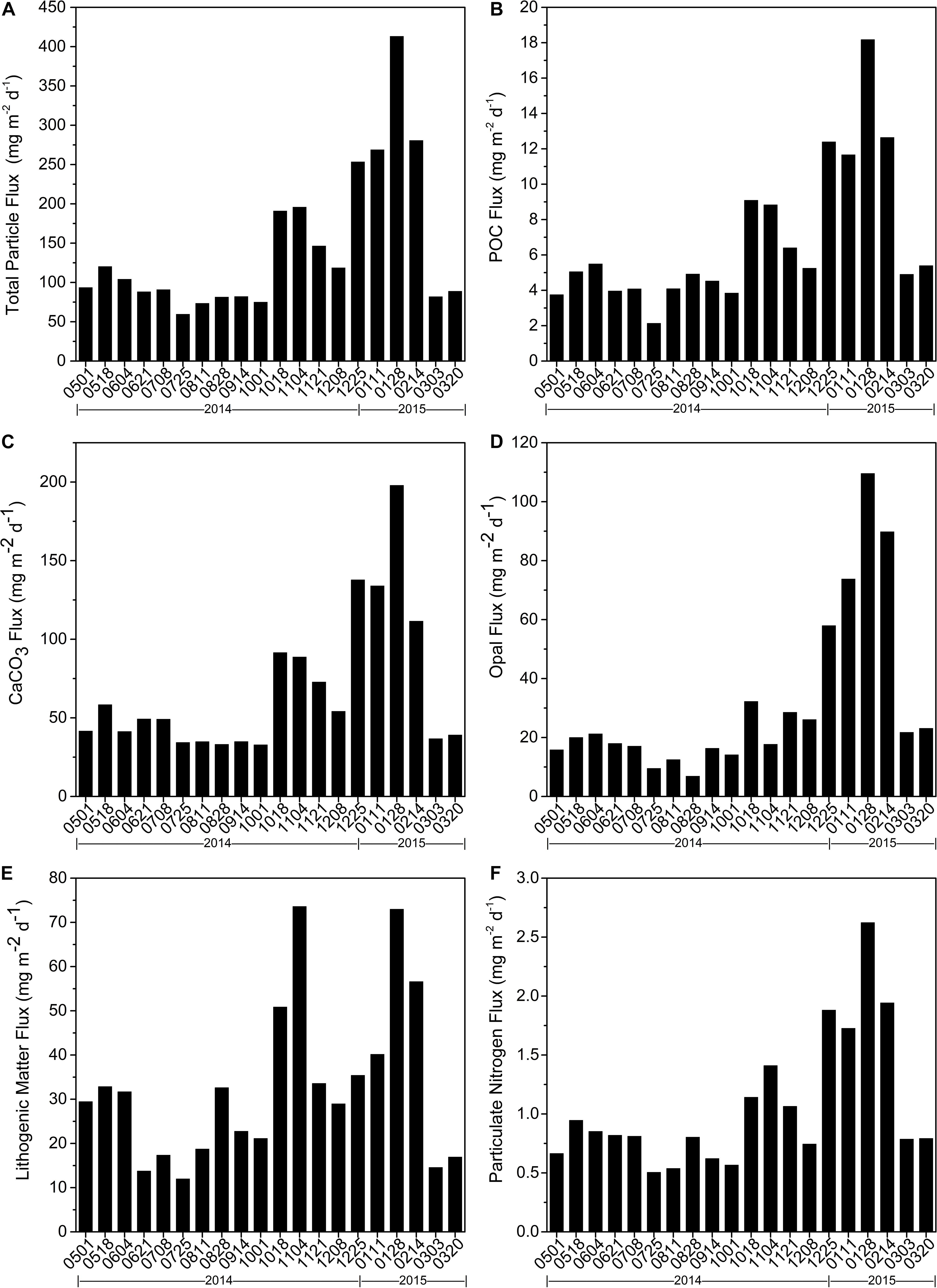
Figure 2. Time Time series of particle fluxes derived from sediment trap at SCS-N station from May 01, 2014 to April 06, 2015. (A) total particle flux, (B) POC flux, (C) CaCO3 flux, (D) opal flux, (E) lithogenic matter flux, and (F) particulate nitrogen flux. Date labels on x axis are marked as mmdd for first date of each sampling period (for this and subsequent similar figures).
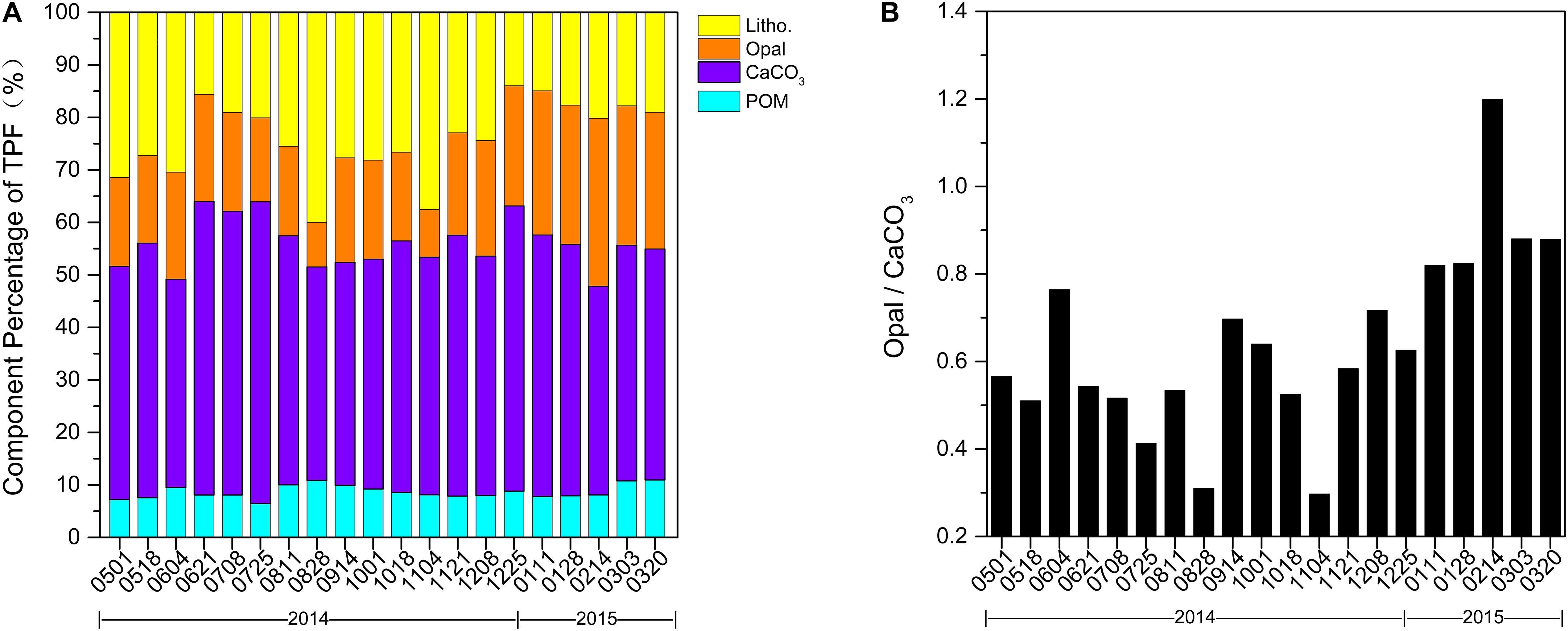
Figure 3. (A) Component percentage of total particle fluxes (TPF) and (B) mole ratio of opal/CaCO3 in sinking particulate fluxes at station SCS-N, May 01, 2014 to April 06, 2015. POM symbolizes particulate organic matter.
Similar to total particulate fluxes, POC, CaCO3, and lithogenic fluxes peaked in winter and autumn, but had small values in summer, with respective ranges 2.1–18.2, 32.9–197.9, and 12.0–73.6 mg m–2 d–1 (Figures 2B,C,E, respectively). The seasonal distributions of POC and CaCO3 fluxes were nearly identical, with both maximizing in January 2015 and a small peak in October (91.5 mg m–2 d–1 for CaCO3 fluxes and 9.1 mg m–2 d–1 for POC) compared to the winter maximum. The only difference was a pronounced minimum of POC fluxes in July, whereas CaCO3 fluxes remained nearly constant with small values over the entire summer. Slightly different from POC and CaCO3 fluxes, two peaks of lithogenic matter fluxes in winter and autumn were essentially equal, and the maximum was in autumn (73.0 mg m–2 d–1 in winter and 73.6 mg m–2 d–1 in autumn). Overall small values of lithogenic material in summer fluctuated noticeably. Similarly, biogenic opal fluxes (Figure 2D) varied from 6.9 to 109.6 mg m–2 d–1, with a prominent peak in winter and minimum in summer. However, the secondary maximum of opal in autumn was barely noticeable compared to other components. Mole ratio of opal/CaCO3 in sinking particulate fluxes is shown in Figure 3B with minimum in November, 2014 and maximum in February, 2015.
Particulate nitrogen fluxes from 28 January through 13 February maximized at 2.6 mg m–2 d–1, and the daily mean from 8 December to 2 March was 1.8 mg m–2 d–1 (Figure 2F). A secondary peak in autumn was also notable, with a range of 1.1–1.4 mg m–2 d–1 and greatest minimum (0.5 mg m–2 d–1) were found during summer (July).
Environmental Parameters
Figure 4 shows seasonal variations of environmental data, including SST, WS, NHF, MLD, NPP, Chl-a concentration, SSHA, AOT, and precipitation. There were distinct winter maxima of WS, MLD, NPP, and Chl-a, with ranges of 2.9–14.3 m s–1, 12.6–53.3 m, 235.9–744.0 mg C m–2 d–1, and 0.02–0.25 mg m–3, respectively. SST showed the minimum in winter and ranges from 21.8 to 29.9°C. NHF and SSHA exhibited analogous cosine patterns. SSHAs were positive from July through November 2014, with a positive maximum in August and negative at other times, with the negative maximum in January (Figure 4G). NHF data were negative from October 2014 through January 2015, with fluctuating positive values in summer (Figure 4C). The distribution of AOT (Figure 4H) was bimodal in autumn (0.18) and winter (0.16), which nearly matched that of lithogenic matter (Figure 2E). Spring had the greatest precipitation (as shown in Figure 4I) compared to other seasons and maximum precipitation (89.0 kg m–2) occurred in June.
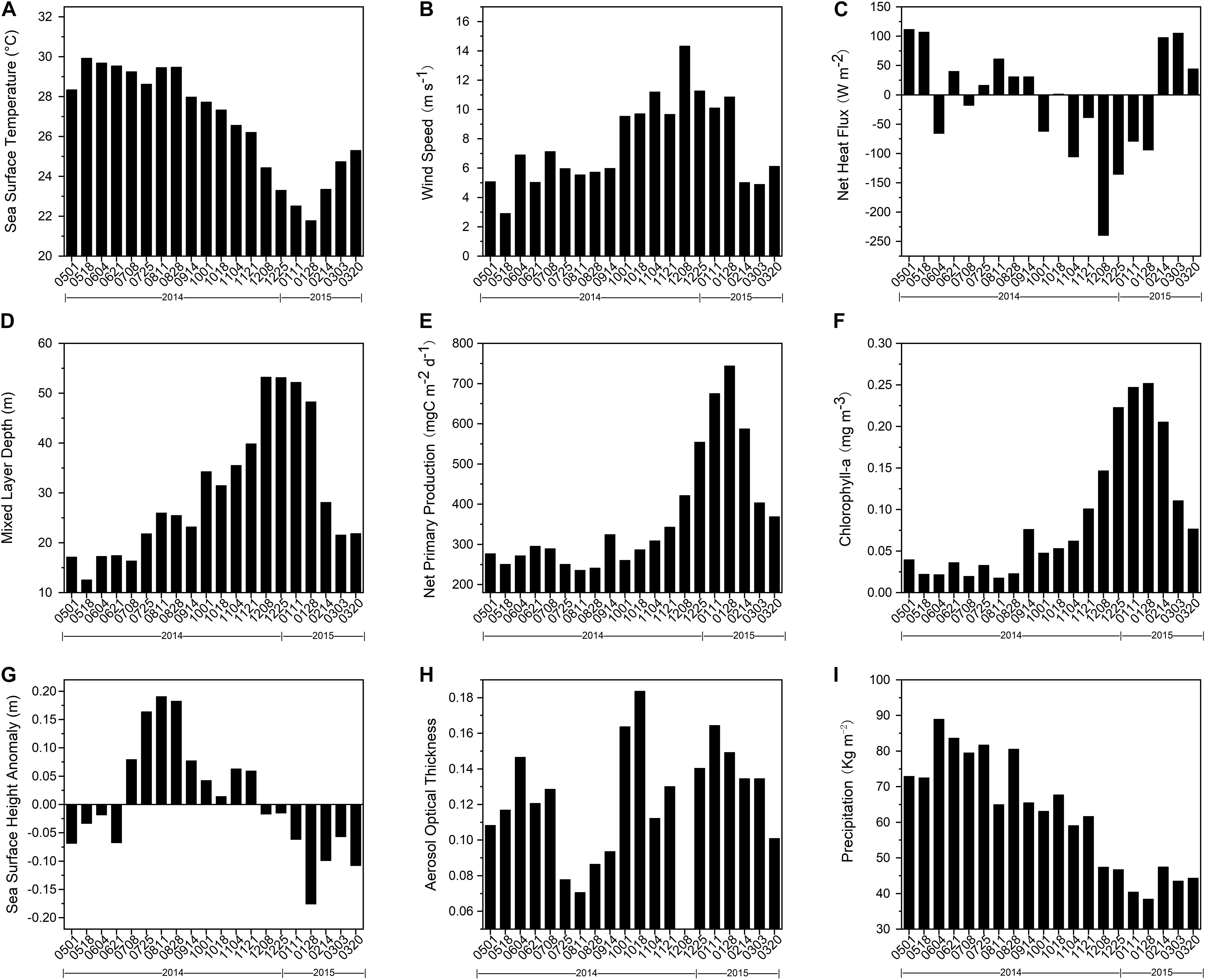
Figure 4. Temporal variations of environmental parameters measured around SCS-N station from May 01, 2014 to April 06, 2015. (A) sea surface temperature, (B) wind speed, (C) net heat flux, (D) mixed-layer depth, (E) net primary productivity, (F) total surface chlorophyll-a concentration (Chlorophyll-a), (G) sea surface height anomaly, (H) aerosol optical thickness, and (I) precipitation.
When the data were analyzed in detail, three periods (1–18 October, 8–24 December, and 28 January to 13 February) were remarkable. First, WS from 1–18 October increased 59% relative to prior levels and NHF changed from negative to positive, both reaching their maximum (absolute) values at the period of 8th to 24th December. The temporal variation of MLD followed those of WS and NHF, with a notable increase of 48% in October and a maximized value (53.3 m) from 8–24 December. But MLD was constantly deeper than 50 m in the following 30 days. SST showed obvious winter minimum while NPP and Chl-a concentration had simple winter peaks with maxima from 28 January to 13 February. The largest negative values of SSHA were also during that period.
Discussion
The vast majority of long-term records of mesopelagic and abyssal fluxes based on sediment traps in the northern SCS have depicted a distinct winter maximum pattern and revealed the great influence of the East Asian Monsoon. However, there are a few physical processes that have a potentially strong impact on carbon export at intra-seasonal to seasonal timescales, and the specific influences of these processes have not been clearly revealed. Therefore, we focused on a 1-year observation of settling particulate fluxes and factors adjusting their temporal variations.
We observed maximum fluxes in winter, a secondary peak in autumn, and an abnormal decline in summer. For example, POC fluxes in winter and autumn were 12.0 and 7.0 mg m–2 d–1, respectively, 1.6 and 1.2 times greater than the fluxes in 2011-2012. Summer POC flux was only 4.0 mg m–2 d–1 in contrast to the 5.1 mg m–2 d–1 in 2011, and was comparable to the flux in the year of El Niño during which the nutrient supply was limited to the photic zone (Tables 1, 2).
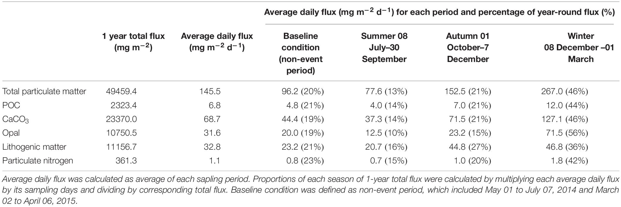
Table 1. Characteristics of seasonal variations of total particles, POC, CaCO3, opal, lithogenic matter and particulate nitrogen fluxes observed at SCS-N station during May 2014 to March 2015.
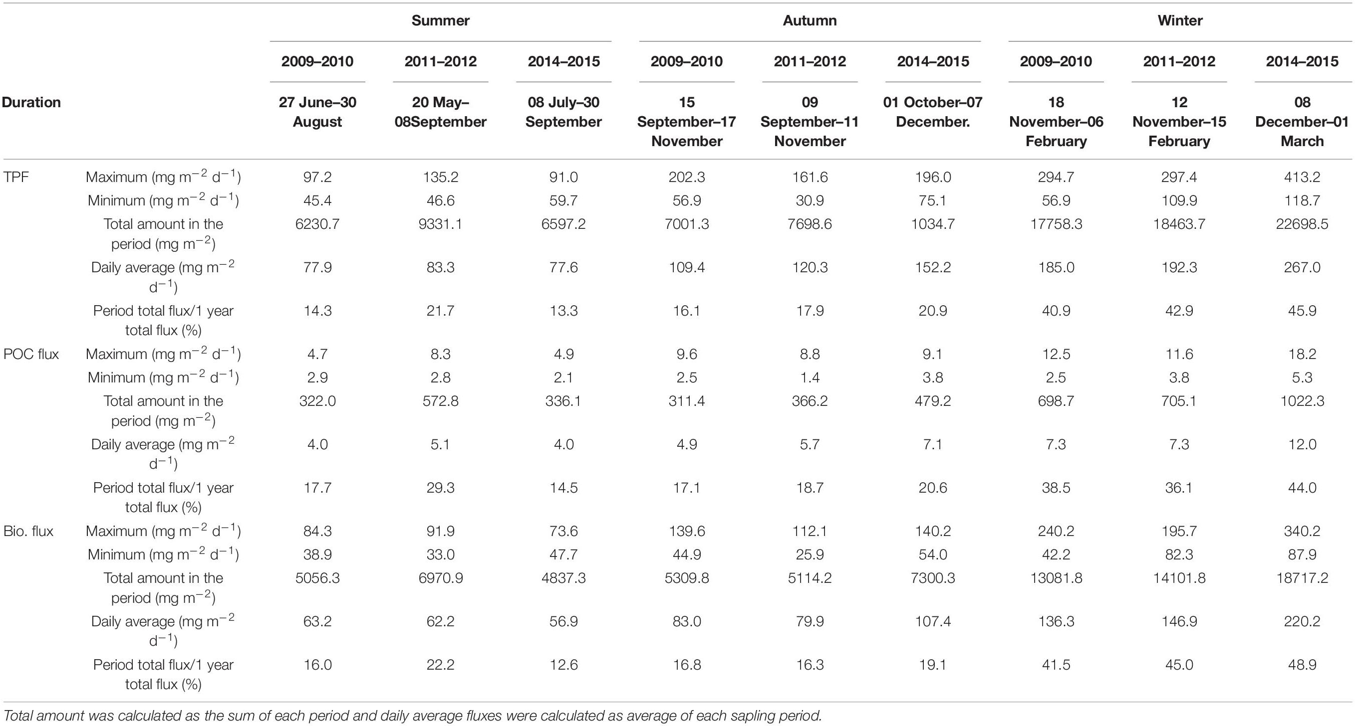
Table 2. Comparison of Total particulate fluxes (TPF), POC fluxes and biogenic matter (Bio., sum of organic matter, CaCO3 and opal fluxes) fluxes calculated for different season in 2014–2015, 2009–2010, 2011–2012 (data from Ran et al., 2015; Priyadarshani et al., 2019).
The obvious seasonal variations raised several questions, as follows. Are the extremely high export fluxes in winter driven by monsoon-induced water mixing and, if so, is this the only control? Why is there a secondary peak during the inter-monsoon period (October to November) and which process plays the major role? What is the forcing mechanism behind the abnormal small values of POC and CaCO3 fluxes on summer monsoon days?
Controls on Peak Flux in Winter
Vertical Mixing
Our trap data and environmental parameters both displayed obvious winter characteristics (Figures 2, 4). The winter monsoon period represented only 25% of the year but accounted for nearly half of the annual measured fluxes: 46% for TPF, 44% for POC flux, 46% for CaCO3 flux, 57% for opal flux, and 36% for lithogenic matter flux (Table 1). TPF, POC, CaCO3, and opal fluxes greatly increased beginning in December by more than 110%, and all components peaked during January 28, to February 13, 2015.
There were also conspicuous increases in environmental data, including WS, MLD, NPP, and surface chlorophyll concentrations. In order to determine the relationship between physical forcing and biogenic activities, we did a Pearson relationship analysis of the data (Table 3). First, the MLD maxima correlated closely with WS (positively) and SST (negatively):
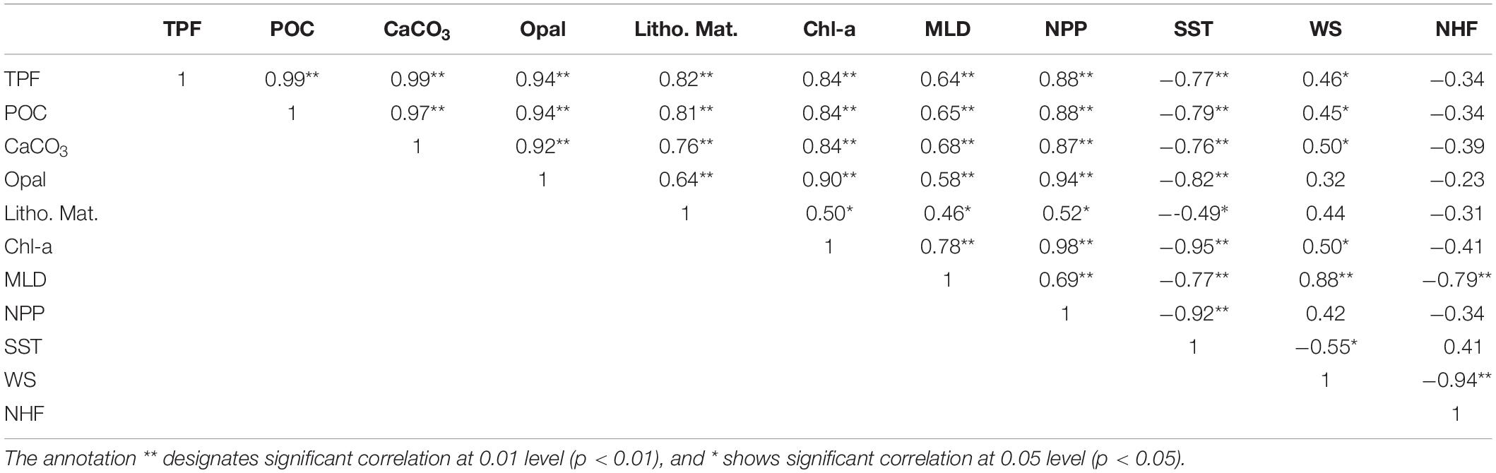
Table 3. Pearson correlation coefficient (R) between daily total particle flux (TPF), particulate organic carbon (POC), CaCO3 fluxes, opal fluxes, lithogenic matter fluxes (Litho. Mat.), surface chlorophyll-a concentration (Chl-a), mixed layer depth (MLD), net primary production (NPP), sea surface temperature (SST), wind speed (WS) and net heat flux (NHF) at SCS-N site.
The multi-linear regression (1) confirmed that the deepening of the mixed layer in the SCS was driven by the combined interaction of convective overturn by surface cooling and wind-induced mixing (Tseng et al., 2005, 2009). The partial correlation coefficients for WS and SST as independent variables to MLD was 0.851 and −0.714 (both P < 0.01, Supplementary Table S3), indicating the dependent influence of these two on the MLD (the analysis process was presented in Supplementary Material).
During the northeast monsoon when the surface water cooled down and the strongest winds occurred over the Strait of Luzon, curving across the SCS basin, the MLD was deepest and broached the nutricline, which was recorded at 60 m year-round at the nearby SEATS station (115.5°E, 18.3°N, 0.5° south of station SCS-N) (Wong et al., 2007). Thus, the strengthened vertical mixing overturned subsurface nutrients into the overlying oligotrophic water and stimulated phytoplankton growth as indicated by maximized Chl-a during December 2014 to January 2015. The correlation between NPP and MLD (r = 0.688, p < 0.01) effectively confirmed the above process. The increase in surface productivity hence generated more numerous downward particles than in any other period.
Our data concurred with discoveries of previous studies in this area. An intensified upward nutrient supply in winter was certified by the increase of δ15N in suspended particulate matter (Kao et al., 2012) and minimum δ13C values with relatively large δ18O values of planktonic foraminifera (Lin et al., 2004, 2011). Primary production rates in winter were estimated at 545.2 ± 408.2 mg C m–2 d–1 (Ning et al., 2004), in contrast with the 465.8 mg C m–2 d–1 annual average at the SEATS station (Ning et al., 2004). About 12% of the primary production (38.4–68.5 mg C m–2 d–1) is said to be exported (Liu et al., 2002), and POC fluxes from the euphotic zone were reported at a large value of 44.4 mg m–2 d–1 in January (Cai et al., 2015). Deep ocean fluxes were recorded at station SCS-N by Lahajnar et al. (2007) during 1987–1988, and by Ran et al. (2015) during 2009–2010. Both showed peak POC fluxes from November through January (4.9 mg m–2 d–1 in 1987 and 12.5 mg m–2 d–1in 2009), in accord with our data for 2014–2015.
However, total particulate fluxes in winter 2014–2015 were much higher in maximum, average daily values and total winter fluxes amount than in 2009–2010 and 2011–2012, as presented by Ran et al. (2015) and Priyadarshani et al. (2019), respectively. The comparison was listed in Table 2. The maximum amount of particulate fluxes in winter was 413.2 mg m–2 d–1 with a daily average of 267.0 mg m–2 d–1 while the maximum values in 2009 and 2011 were 294.7 and 297.4 with a daily average of 185.0 and 192.3 mg m–2 d–1, respectively. The winter period daily flux in POC and opal in 2014 were 1.7- and 1.5-fold to those in 2009 (7.3 mg m–2 d–1 for POC and 48.2 mg m–2 d–1 for opal fluxes, respectively) (Priyadarshani et al., 2019). Despite the fact that the winter period in 2014 (85 days) was shorter than in 2009 and 2011 (96 days), POC flux in winter 2014 accounted for 44% of annual total POC flux and was larger than those in 2009 and 2011 (38 and 36%, respectively). In contrast to the strengthened sediment fluxes, the environmental parameters showed little differences. The average annual wind speed was comparable (7.1 m s–1 for 2009–2010 and 7.6 m s–1 for 2014–2015), indicating little difference in monsoon strength. MLD were around 50 m for both 2009–2010 and 2014–2015. The MLD was even deeper in the winter of 2011–2012 (>70 m) (Priyadarshani et al., 2019). Thus, the question arose as to why the fluxes in 2014 were so much higher than other years under similar monsoon conditions.
Additionally, there were slight mismatches in the timing of MLD, Chl-a, and downward fluxes, whereas there were good time relations in previous years (Ran et al., 2015; Li et al., 2017; Priyadarshani et al., 2019). No distinct time lag (longer than 1 month) here may be owing to a characteristic of marginal sea where huge terrestrial materials in the particles are large enough to accelerate the settling velocity (Goutx et al., 2007). The time mismatches in our study were too obvious to be ignored. First, the maximum surface Chl-a concentration occurred between 28 January and 13 February, about 34 days after the MLD maximum in December. In both 2009–2010 and 2011–2012, surface Chl-a concentration changed almost immediately when MLD changed during winter time (Priyadarshani et al., 2019). Second, bulk fluxes were collected in mid-to-late February, showing POC fluxes at 12.6 mg m–2 d–1 (Figure 2B) with a MLD just greater than 20 m (Figure 4D). In the meantime opal flux was the second highest of the year (Figure 2D), and Chl-a concentration was 0.21 mg m–3 (Figure 4F), 133% greater than average of 0.09 mg m–3. Logically, nutrients cannot be effectively transported by a shoaled MLD, so productivity and export should have been cut off. If the high fluxes collected over the 1,000 depth are caused by the delayed settlement progress in the previous winter bloom, then the high chlorophyll value in the surface layer is contradictory. All these unusual phenomena leave the possibility of another positive mechanism for downward particles superimposed on the primary role of the northeast monsoon.
Cyclonic Eddy
What factors could have contributed to a higher flux than the previous year and the mismatch in timing of the MLD, Chl-a, and downward fluxes.
Mesoscale cyclonic eddies, which can transport nutrients to the surface layer by upwelling within the eddy center (McGillicuddy et al., 1998), seemed to be possible. Indeed, a strong cyclonic eddy appeared to have occurred during the period in the northern SCS, according to subtractive SSHA (Figure 4G). Using a manual method of eddy tracking, a relatively large mesoscale eddy (radius = 48–174 km) formed northwest of Luzon Island during mid-December 2014 (Figure 5A). This eddy matured about 20 days later and began to split into small eddies during early-to-mid January. During this period the eddy moved westward, but our station was out of its control. It wasn’t until 22 January that the eddy exerted an influence on our station (Figure 5B), as shown by a sharp decrease (by 16%) in daily SSHA at SCS-N. One of the small cyclonic eddies that split from the northwest part of the large eddy developed very near our sampling station, beginning 26 January. The central part of the small eddy reached SCS-N in early February during its mature stage (Figure 5C). The station SSHA was <−0.18 m beginning 2 February and the minimum SSHA (−0.20 m) appeared between 7 and 9 February (Figure 6). This cold-core eddy continued to influence our station through 27 February (Figures 5D, 6). The close match between the kinetic energy of this small eddy and the negative SSHA of our sampling station is a strong indication of cyclonic effects (Figure 6).

Figure 5. Satellite images of daily sea surface height anomaly (SSHA, m) in northern SCS from AVISO product on (A) December 28, 2014, (B) January 22, 2015, (C) February 09, 2015, and (D) February 27, 2015, exhibiting cyclonic eddy activity during winter period of 2014–2015 in study area. Dots on map represent 1/4° × 1/4° grid around station SCS-N and gray line with label 2,000 indicates water isobaths of 2,000 m.
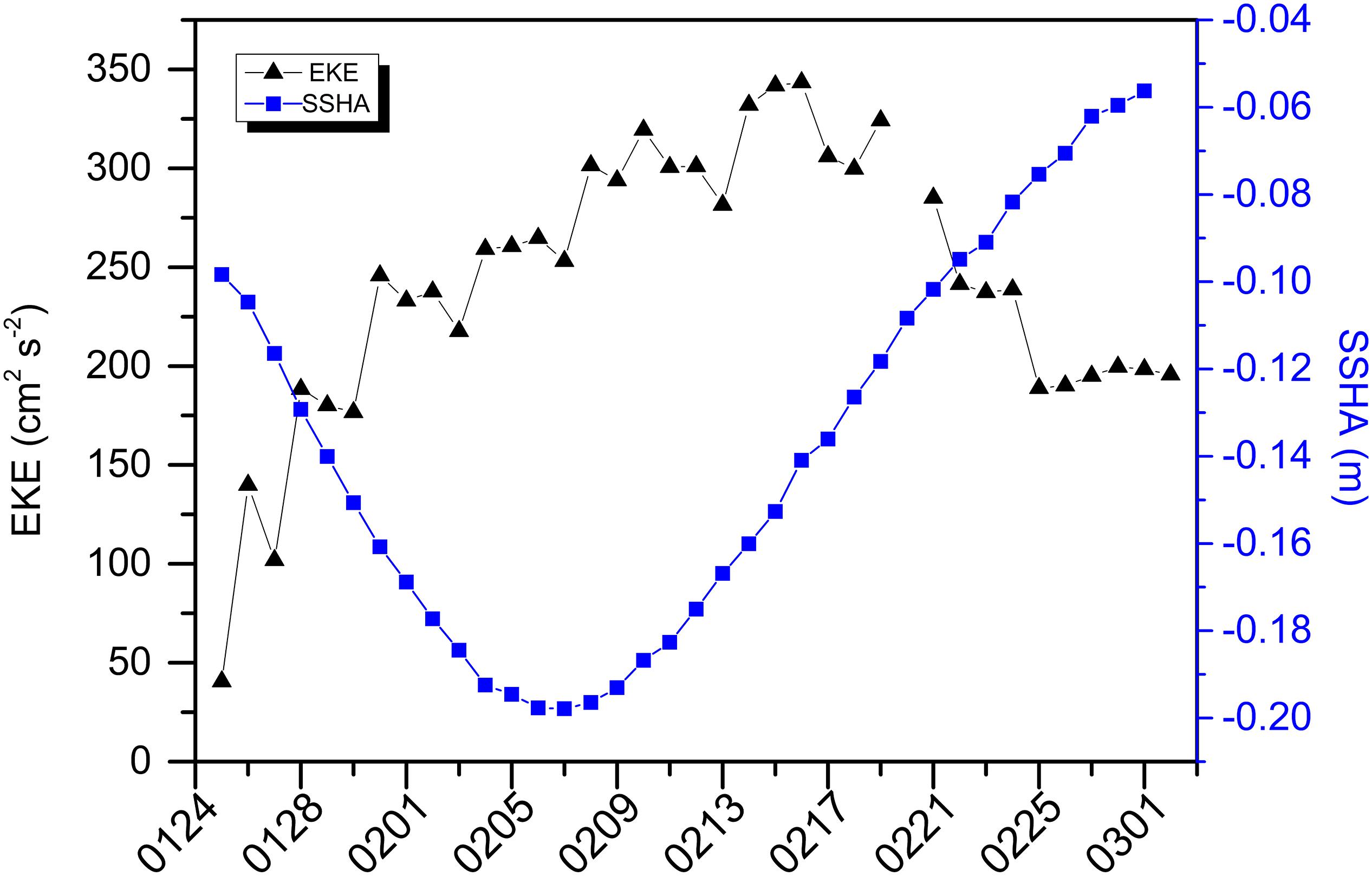
Figure 6. Variations of eddy kinetic energy (EKE) at center of relatively small mesoscale cyclonic eddy (split from the original large one) near station SCS-N, using manual tracking method and daily sea surface height anomaly (SSHA) of 1/4° × 1/4° grid area around sampling station from January 25, to March 02, 2015.
Cyclonic eddies could remarkably increase surface biomass (Chen et al., 2007; Xiu and Chai, 2011; Wang et al., 2016; Honda et al., 2018). Positive Chl-a anomalies from 1998 to 2011 were associated with cyclonic eddies in the SCS (He et al., 2016). There is phytoplankton enhancement of 10.5% in total Chl-a biomass in water column at the surface layer within the eddy center of SSHA < 0.20 m (Wang et al., 2016). Elevation in productivity caused by cyclonic eddies in spring could even catch up with the maximum level in winter in SCS (Chen et al., 2007).
In our sampling winter period, from the end of January through mid-February, the SCS-N station was affected by a combination of cyclonic eddies and northeast monsoons. Under the resultant strong vertical mixing, the accelerated upward nutrient transport caused by eddy pumping allowed for deeper nutrient replenishment in the mixed layer (He et al., 2016). This replenishment of nutrient conspicuously increased productivity within the euphotic layer and contributed to a higher level in fluxes compared with previous years. Then, from mid-to-late February when the MLD seemed to be shoaled, our station was directly under the eddy center upwelling area. It was found that the water column-integrated biomass of diatoms was 21.3-fold greater at the center of a cyclonic eddy relative to its outside (Wang et al., 2016). The direct nutrient input by upwelling stimulated the growth of phytoplankton in the upper layer as observed in the high concentration of surface chlorophyll, leading to the strong fluxes seen during the sampling period from 14 February through 1 March. The upwelling effect of the cold water may also make the potential temperature line move upward, thus the MLD resulting from potential temperature seems to be shoaled. Further, one biological signal of the cold-core eddy is that it functioned preferentially as a selective silica pump (Thunell et al., 2007), although calcareous plankton may also benefit. Li et al. (2017) revealed that the cyclonic eddy in the SCS could contribute to 44–59% of opal and 17–54% of POC fluxes. The daily average opal fluxes in winter in our sampling time was 71.5 mg m–2 d–1 with a percentage of period to the annual amount as 56% in contrast to the number of 48.2 mg m–2 d–1 (43%) in 2009–2010 and 49.2 mg m–2 (44%) in 2011–2012 (Priyadarshani et al., 2019). The period daily average flux of CaCO3 also increased to 127.1 mg m–2 d–1 in contrast to 74.9 mg m–2 d–1 (2009-2010) and 84.4 mg m–2 d–1 (2011-2012), while the percentage of period to the annual amount in CaCO3 showed little difference (41-48%). The mole rate of opal/CaCO3 was over 0.8 since January and the maximum of 1.3 appeared in mid-to-late February (Figure 3B). The maximized biological signal of cyclonic eddies in mid-to-late February was due to the direct influence of eddy upwelling and the weakened monsoon wind. Thus, this mechanism allowed a clear interpretation of secondary maximum opal flux (89.8 mg m–2 d–1) and the maximum mole rate of opal/CaCO3 (Figure 3B) during mid-to-late February, when the MLD was shallower than 20 m.
Compared with previous years, stronger signal in SSHA was recorded in our sampling year (2014–2015). SSHA data in 2009 and 2011 were >−0.10 m during the winter monsoon period (Ran et al., 2015; Priyadarshani et al., 2019). The larger fluxes in the winter of 2014-2015 compared to previous years were well interpreted by the extra replenishment of nutrients upwelled by cyclonic eddy.
Apart from cold-core eddy, atmospheric aerosol deposition may be another candidate, because strong flux of lithogenic matter and increased aerosol thickness were observed in winter (Figures 2E, 4H). However, little precipitation in the study period impeded atmospheric aerosol reaching the ocean surface (Figure 4I). Wet deposition was reported to be the main route for atmospheric deposition in the area (Jung et al., 2011). So, the atmospheric aerosol deposition wasn’t the answer to our findings in winter.
A third possibility lies in lateral transportation from the river and the Luzon Strait. First, our study site is distant from any river influence (Wong et al., 2007). In addition, water in the Luzon Strait comes from the West Pacific and has more oligotrophic characteristics than the SCS. An export of 1 × 10¹¹ mol year–1 of phosphate and 1.4 × 10¹² mol year–1 of nitrate is estimated from the SCS to the western Philippine Sea at intermediate depths between 350 and 1,350 m (Chen et al., 2001). Low nutrients cannot support the bloom of diatom and transport as large a flux of opal. However, the ratio of opal/CaCO3 (Figure 3B) in our recorded fluxes peaked in February 2015, which showed a large amount of diatom growth. Therefore these particles weren’t attributed to lateral transportation from the Luzon Strait.
In summary, the winter peak flux in our data was the result of vertical mixing from convective overturn and monsoon, overlapped with a mesoscale cyclonic eddy. Vertical mixing by the winter monsoon played the critical role, while the cold-core eddy also had positive effects. It was precisely because of the coincidence of these factors that winter fluxes during 2014–2015 were much stronger than in previous years. Unfortunately, the contributions of those factors remain uncertain and more research, including in situ observation, is necessary for more detailed exploration.
Autumn Secondary Maximum Fluxes Owing to Aerosol Deposition
TPF, CaCO3 flux, and POC flux showed pronounced secondary maxima during the autumn inter-monsoon. Daily average fluxes were 152.2, 71.5, and 7.0 mg m–2 d–1 for TPF, CaCO3, and POC fluxes, surpassing values in non-event periods (including May 01–July, 07, 2014 and March 02–April, 06, 2015) by 58, 61, and 48%, respectively (Table 1). The lithogenic flux was even maximized in November (73.6 mg m–2 d–1). This is a very interesting phenomenon, different from other observations of small values in autumn. Lahajnar et al. (2007) and Ran et al. (2015) indicated TPF and POC autumn fluxes of less than 100 and 4 mg m–2 d–1, respectively. At this time, the mixed layer was mostly shallower than 40 m, despite a slight deepening compared to summer, but this was much shallower than the top of the nutricline depth (50–70 m) measured at the SEATS station (Wong et al., 2007). It was impossible to support upper production through reverse mixing of subsurface nutrients, and the tiny fluctuation in sea level further excluded the influence of mesoscale eddies.
The main sources of lithogenic matter are river input, atmospheric deposition, and sediment re-suspension. First, our study site is distant from any river influence (Wong et al., 2007). The most influential river emptying into the northern part of the SCS was Pearl River, with flow rates of 316 km3 year–1 reaching the SCS at 22°N (Wong et al., 2007). The lesser rivers that flow into the SCS in the Hainan and Taiwan islands were the Wanquan river and the Choshui river with an annual flow of 5.8 and 5.2 km3 year–1 (Liang and Ye, 2015), and the Cagayan Rio River which empties into the SCS from Luzon Island. The distance between the estuary of Pearl River, Cagayan Rio River, Wanquan River, Choshui River, and our site were 515.3, 478.4, 590.8, and 738.8 km, respectively. The basin-wide circulation gyres effectively isolate the interior of the SCS proper from the influence of the land-runoff (Wong et al., 2007). Moreover, although most lithogenic matter in the northern SCS might result from modern transport and the resuspension of sediments by the Kuroshio intrusion along the Taiwan Strait (Liu et al., 2014), there was little seasonal variability (especially during the autumn peak) in the upper layer. Therefore, atmospheric deposition was the most likely source of the sharp increase (2.4-fold) in autumn lithogenic matter. The pattern of lithogenic flux was in phase with aerosol optical thickness (Figure 4H), in which large amounts of airborne particles were observed during autumn. These atmospheric aerosol particles could effectively deposit to the ocean surface via relatively frequent precipitation (59.1–67.7 kg m–2) as shown in Figure 4I.
Our data are consistent with Lin et al. (2007), who showed a powerful influence of atmospheric deposition in the study area, relating it to a northern source of eastern China fossil fuel together with Asia Desert Dust. Large-scale combustion of biomass usually takes place in October, and fossil fuel aerosol contains large amounts of nitrogen which acts as a direct source of nutrient input (Zhang et al., 2018). Additionally, micronutrients like iron in desert dust that are deposited on the ocean surface in the form of bioavailable Fe(II) can trigger upper-ocean nitrogen fixation (Chavagnac et al., 2007). This fixation can convert di-nitrogen to fixed nitrogen in the presence of iron and lead in order to increase phytoplankton biomass. Strong nitrogen fixation in the SCS that can support 3–13% of net primary production was revealed by Wong et al. (2002) at the SEATS station, and the availability of iron during seasons of strong aerosol deposition could substantially enhance nitrogen fixation (Wong et al., 2007). The increased percentage of PN in biogenic matter during autumn (0.99%, Table 4) was 22.2% greater than average in the winter high-flux period (0.81%), which might indicate strengthened primary production caused by nitrogen fixation. From a microcosm incubation experiment with aerosol event scales on deck, Guo et al. (2012) observed positive responses in biomass in the SCS and a shift in dominant phytoplankton assemblages from picoplankton to microphytoplankton (Guo et al., 2012). According to model data in the SCS, enhancement of Chl-a during a dust event and dust deposition could contribute ∼20% of annual biological new production (Kim et al., 2014). A strong association between Chl-a and AOT variability in non-winter months at the SEATS station was presented by Lin et al. (2009), implying an important role for aerosol input in the northern SCS. The absence of large values of surface Chl-a concentration in our remote-sensing data may be attributed to a limitation of satellite observation, meaning the subsurface water bloom cannot be detected. The subsurface chlorophyll maximum was distinct in the nearby SEATS station (Gong et al., 2014) and different physical processes may enhance the phenomenon in the SCS (Chen et al., 2006; Lu et al., 2010).

Table 4. Biogenic matter fluxes in sinking particles (calculated as sum of organic matter, CaCO3, and opal fluxes) and particle composition of particulate nitrogen (PN) in biogenic matter fluxes during different seasons of 2014–2015.
Additionally, same as biogenic minerals, lithogenic minerals in surface water could have a ballasting effect in the form of increasing the sedimentation rate of particulate matter and protecting organic matter from decomposition in marginal seas (Fischer and Karaka, 2009). The composition percentage of total particle fluxes in Figure 3A effectively confirms this. Although CaCO3 was the most abundant component of particles during most of the year, the proportion of lithogenic matter increased from 27 to 38% in autumn. This increase was because of the effect of substantial atmospheric loading on the stimulation of primary production and further aggregated with organisms settling into the deep sea. Our data corresponded to the findings of Lee et al. (2009) for the Mediterranean Sea, which revealed that dust greatly increased downward export flux by particle aggregation. In the low-nutrient low-chlorophyll area where there is a definite fertilization effect by dust, >50% of the increase in particulate organic matter was related to the aggregation process (Bressac et al., 2013).
The autumn secondary peak occurred for every flux except that of opal, and there was a minimum of opal/CaCO3 in early November. There are two potential reasons for this. The first is that airborne aerosol might be more likely to promote the growth of calcareous organisms than siliceous plankton. This was supported by the fact that the daily average CaCO3 flux in autumn was 1.6-fold to the baseline value (Table 1, baseline condition was defined as non-event period, which included May 01 to July 07, 2014 and March 02 to April 06, 2015). The second reason is related to the various ballasting effects from different types of minerals (Salter et al., 2010). Carbonate was important in increasing particle density and thus accelerated the sinking of particles while most of the aggregate formed by opal was re-mineralized before reaching the bottom (Francois et al., 2002). Hence, opal does not increase organic matter flux as effectively as carbonate.
Our study highlights the vital function of aerosol deposition for carbon export in the form of nutrient replenishment, improvement of nitrogen fixation, and strengthening of the ballasting effect via extra lithogenic mineral supply in the marginal sea. Limited by sparse in situ data from a time-series observation of vertical particle flux below the euphotic layer, investigation of the mineral ballast effect and atmospheric particle deposition is still in its infancy, so further research is recommended.
Small Values in Summer Induced by Anticyclonic Eddy
During the summer monsoon (June–September), total particle, POC, and lithogenic matter fluxes showed clear minima of 59.7, 2.1, and 12.0 mg m–2 d–1 in July, and a minimal opal flux of 6.9 mg m–2 d–1 in August. The average summer daily TPF was 77.6 mg m–2 d–1, in contrast with the annual daily average of 145.5 mg m–2 d–1. Furthermore, the daily average biological flux in summer was 56.9 mg m–2 d–1, contributing only 13% to the annual figure, while in the previous years the value was 63.2 and 62.2 mg m–2 d–1 with an annual percentage of 16 and 23% for 2009 and 2011 (Priyadarshani et al., 2019), respectively.
Very few factors substantially suppressed carbon export, except for the mesoscale anticyclonic eddy (Lasternas et al., 2012). Our SSHA data (Figure 4G) exceeded 0.07 m at the beginning of July, directly suggesting the influence of the anticyclonic eddy (Roemmich and Gilson, 2001; Huang et al., 2010). As shown in Figure 7, the sampling station was affected by a mesoscale warm-core eddy moving from south to northwest, beginning July 14. The station was at the eddy center from August 9, with a maximum sea level anomaly of 0.19 m. This eddy lasted 1 month and began to dissipate in September. The characteristics of central downwelling (Samuelsen et al., 2012) within the anticyclonic eddy weakened the upward nutrient transportation, thus led to the small values of fluxes in summer.
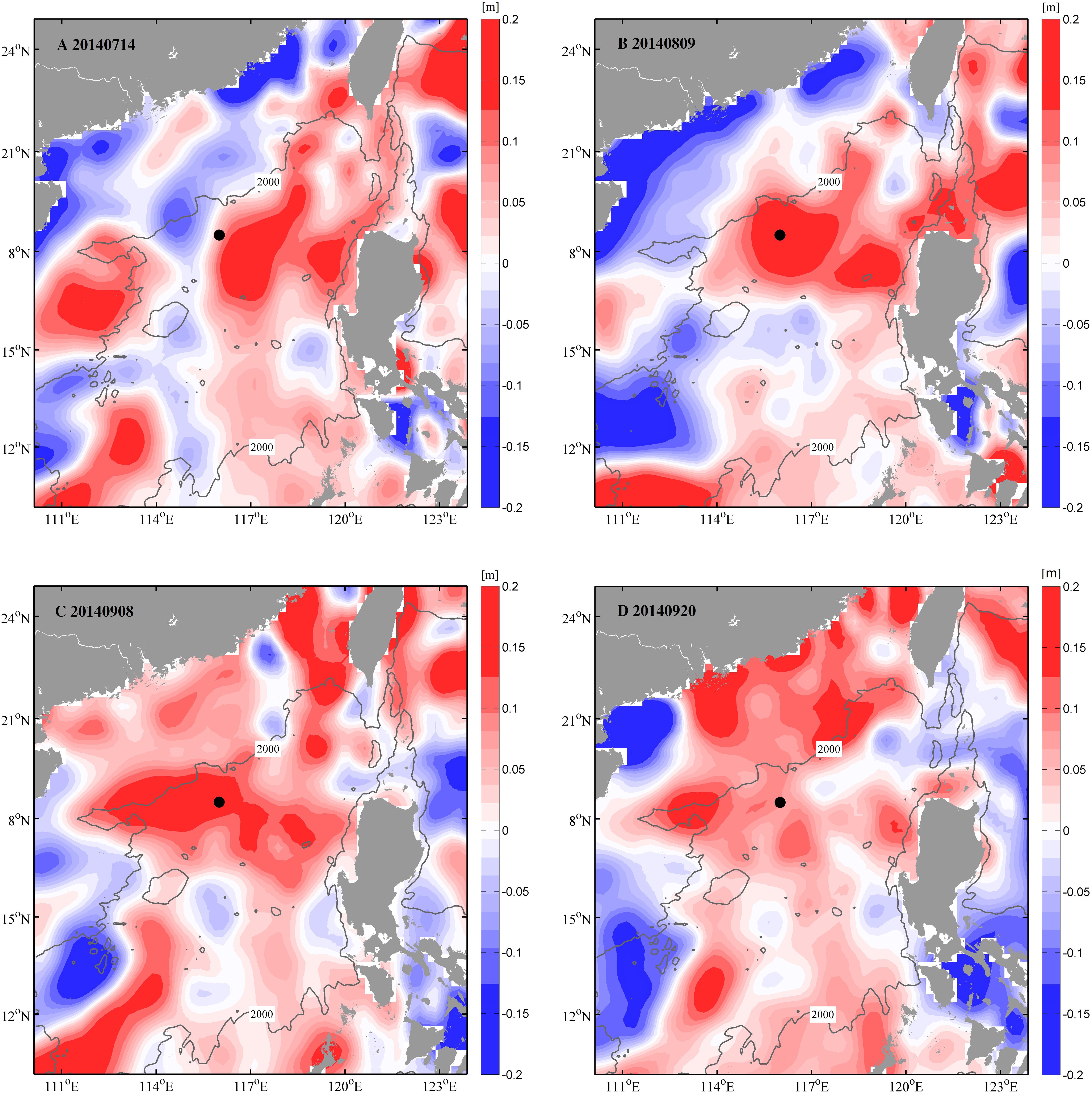
Figure 7. Satellite images of daily sea surface height anomaly (SSHA, m) in northern SCS from AVISO product on (A) July 14, 2014, (B) August 09, 2014, (C) September 08, 2014, and (D) September 20, 2014, exhibiting anticyclonic eddy activity during summer period of 2014 in study area. Black dots on map represented 1/4° × 1/4° area around station SCS-N. Gray line with label 2,000 indicates water isobaths of 2,000 m.
Based on the Bermuda Atlantic Time-series Study of the Sargasso Sea, Sweeney et al. (2003) clearly showed that the 1994 spring bloom was suppressed by the passage of anticyclonic eddies with SSHA around 0.20 m. In the Norwegian Sea, warm-core eddies could delay the phytoplankton bloom by about 2 weeks (Hansen et al., 2010). Lasternas et al. (2012) not only observed a considerable enhancement of dissolved organic carbon (DOC) concentration in the anticyclonic eddy center, but also diatom cell mortality rates of 60%. They proposed that the high mortality and cell lysis rates mainly resulted in the DOC increase, thereby reducing carbon export. This is consistent with Moutin and Prieur (2012) and Bressac et al. (2013) for the Mediterranean, emphasizing weak primary production and carbon export but large values of DOC concentration in anticyclonic eddies. Although the anticyclonic eddy was revealed to have a positive biological effect within the subtropical gyre (Dufois et al., 2016), the negative relative difference Rd (%) in Dufois’s research of the northern SCS indicated the counteraction of the anticyclonic eddy. The SCS is a typical surface oligotrophic and low-productivity area in which productivity is mainly fueled by various physical processes providing nutrients to the upper layer. The characteristic downward flow in an anticyclonic eddy center substantially inhibits the growth of phytoplankton (Xiu and Chai, 2011; Guo et al., 2015). The model data of Ning et al. (2004) indicate that a warm-core eddy can reduce phytoplankton growth by 31%.
Unlike anticyclonic eddies, other processes like typhoon, monsoon, and dust deposition can only supply nutrients to the surface other than restrain. Furthermore, there were no major differences in environmental data of WS and NHF compared with the 2009–2010 data of Ran et al. (2015), apart from conspicuously large values of SSHA. This reflected the only influence of warm-core eddy.
There is a secondary peak of carbon output during the summer monsoon in some long-term records from the SCS (Chung et al., 2004; Li et al., 2017), in contrast with our study. However, these records are from the central basin area where the southwestern monsoon has a strong impact. Our study site was in the northern SCS, outside the summer circulation area (Shaw and Chao, 1994), and there was little impact from upwelling (Liu et al., 2002; Ning et al., 2004). Moreover, there were no apparent summer features in studies of the nearby SEATS station (Tseng et al., 2005; Wong et al., 2007). The small summer export value in the present study is likely attributable to the influence of the mesoscale anticyclonic eddy.
Conclusion
Total particle flux, particulate organic carbon, CaCO3 and lithogenic fluxes peaked in winter and autumn, but exhibited minima in summer. Opal flux was similar to those fluxes, with a prominent maximum in winter and a minimum in summer, whereas a secondary maximum of opal in autumn was barely noticeable compared with other components. A deeper mixed layer was related to the northeast monsoon and surface cooling, overlapped with the cyclonic eddy effect, which may be responsible for the strong winter fluxes. However, an anticyclonic eddy would suppress the subsurface nutrient supply, primary production, and subsequent export flux in summer. With respect to the autumn flux peaks of lithogenic and CaCO3, the scavenging of atmospheric particles and mineral ballast effect are potential causes. Our study highlights that in addition to monsoonal transition, intra-seasonal physical processes (e.g., mesoscale eddies and aerosol deposition) are important to deep particle fluxes in the SCS.
Data Availability Statement
The raw data supporting the conclusions of this article will be made available by the authors, without undue reservation, to any qualified researcher.
Author Contributions
ST analyzed the data and led the writing of the manuscript under the instruction of JC and HL. JZ and LS accomplished the laboratory work with the cooperation of MW. ZW provided some environmental parameter data and contributed to track eddies by manual methods. MW and HZ made modifications for the manuscript.
Funding
This study was carried out in the financial support of the State Key R&D Project of China (2016YFA0601101), the National Natural Science Foundation of China (41906045 and 91528304), the Special Fund for Basic Scientific Research of the Second Institute of Oceanography, Ministry of Natural Resources (JT1501 and JG1514), and the Project of State Key Laboratory of Satellite Ocean Environment Dynamics, Second Institute of Oceanography, MNR (SOEDZZ1901), and the National Program on Global Change and Air-Sea Interaction (GASI-03-01-06-02).
Conflict of Interest
The authors declare that the research was conducted in the absence of any commercial or financial relationships that could be construed as a potential conflict of interest.
Acknowledgments
We are grateful to Institute of Geology, University of Hamburg for helpful instructions and laboratory cooperation in elemental analysis and the crews of R/V Tianying for their assistance during the mooring deployment. We appreciate the National Oceanic and Atmospheric Administration for providing SST, WS, and NHF data; Ocean Productivity for providing MLD and NPP data (http://orca.science.oregonstate.edu); National Aeronautics and Space Administration for providing AOT data; Asia-Pacific Data Research Center for providing precipitation water data (http://apdrc.soest.hawaii.edu); and Reiner Schlitzer with his group for sharing the Ocean Data View graphics program (odv.awi.de). We would like to thank LetPub (www.letpub.com) for providing linguistic assistance during the preparation of this manuscript.
Supplementary Material
The Supplementary Material for this article can be found online at: https://www.frontiersin.org/articles/10.3389/feart.2020.00074/full#supplementary-material
Footnotes
- ^ https://scripps.ucsd.edu/programs/keelingcurve/
- ^ http://www.ncdc.noaa.gov/
- ^ http://orca.science.oregonstate.edu
- ^ https://oceancolor.gsfc.nasa.gov
- ^ https://www.aviso.altimetry.fr
- ^ http://apdrc.soest.hawaii.edu
References
Archer, D., and Maier-Reimer, E. (1994). Effect of deep-sea sedimentary calcite preservation on atmospheric CO2 concentration. Nature 367, 260–263. doi: 10.1038/367260a0
Armstrong, R. A., Lee, C., Hedges, J. I., Honjo, S., and Wakeham, S. G. (2002). A new, mechanistic model for organic carbon fluxes in the ocean based on the quantitative association of particulate organic matter with ballast minerals. Deep Sea Res. 49, 219–236. doi: 10.1016/s0967-0645(01)00101-1
Barker, S., Higgins, J. A., and Elderfield, H. (2003). The future of the carbon cycle: review, calcification response, ballast and feedback on atmospheric CO2. Philos. T. R. Soc. A: Math. Phys. Eng. Sci. 361, 1977–1998. doi: 10.1098/rsta.2003.1238
Bressac, M., Guieu, C., Doxaran, D., Bourrin, F., Desboeufs, K., Leblond, N., et al. (2013). Quantification of the lithogenic carbon pump following a dust deposition event. Biogeosci. Discuss. 10, 13639–13677. doi: 10.5194/bgd-10-13639-2013
Broecker, W. S. (1982). Ocean chemistry during glacial time. Geochim. Cosmochim. Acta 46, 1689–1705. doi: 10.1016/0016-7037(82)90110-7
Cai, P., Zhao, D., Wang, L., Huang, B., and Dai, M. (2015). Role of particle stock and phytoplankton community structure in regulation particulate organic matter export in a large marginal sea. J. Geophys. Res. Oceans 120, 2063–2095. doi: 10.1002/2014JC010432
Chavagnac, V., Waniek, J. J., Atkin, D., Milton, J. A., Leipe, T., Green, D. R. H., et al. (2007). Anti-Atlas Moroccan Chain as the source of lithogenic-derived micronutrient fluxes to the deep Northeast Atlantic Ocean. Geophys. Res. Lett. 34:L21604. doi: 10.1029/2007GL030985
Chen, C., and Wang, G. (2015). Interannual variability of the eastward current in the western South China Sea associated with the summer Asian monsoon. J. Geophys. Res. Oceans 119, 5745–5754. doi: 10.1002/2014JC010309
Chen, C. C., Shiah, F. K., Chung, S. W., and Liu, K. K. (2006). Winter phytoplankton blooms in the shallow mixed layer of the South China Sea enhanced by upwelling. J. Mar. Syst. 59, 97–110. doi: 10.1016/j.jmarsys.2005.09.002
Chen, C. T. A., Wang, S. L., Wang, B. J., and Pai, S. C. (2001). Nutrient budgets for the South China Sea basin. Mar. Chem. 75, 281–300. doi: 10.1016/s0304-4203(01)00041-x
Chen, Y. L. L., Chen, H. Y., Lin, I. I., Lee, M. A., and Chang, J. (2007). Effects of cold eddy on phytoplankton production and assemblages in Luzon strait bordering the South China Sea. J. Oceanogr. 63, 671–683. doi: 10.1007/s10872-007-0059-9
Chung, Y., Chang, H. C., and Hung, G. W. (2004). Particulate flux and 210Pb determined on the sediment trap and core samples from the northern South China Sea. Cont. Shelf Res. 24, 673–691. doi: 10.1016/j.csr.2004.01.003
Duce, R. A., and Tindale, N. W. (1991). Atmospheric transport of iron and its deposition in the ocean. Limnol. Oceanogr. 36, 1715–1726. doi: 10.4319/lo.1991.36.8.1715
Dufois, F., Hardman-Mountford, N. J., Greenwood, J., Richardson, A. J., Feng, M., and Matear, R. J. (2016). Anticyclonic eddies are more productive than cyclonic eddies in subtropical gyres because of winter mixing. Sci. Adv. 2:e1600282. doi: 10.1126/sciadv.1600282
Eppley, R. W., and Peterson, B. J. (1979). Particulate organic matter flux and planktonic new production in the deep ocean. Nature 282, 677–680. doi: 10.1038/282677a0
Fischer, G., and Karaka, G. (2009). Sinking rates and ballast composition of particles in the Atlantic Ocean: implications for the organic carbon fluxes to the deep ocean. Biogeosciences 6, 159–160. doi: 10.5194/bg-6-85-2009
Francois, R., Honjo, S., Krishfield, R., and Manganini, S. (2002). Factors controlling the flux of organic carbon to the bathypelagic zone of the ocean. Glob. Biogeochem. Cycle 16, 34–31. doi: 10.1029/2001GB001722
Gaye, B., Wiesner, M. G., and Lahajnar, N. (2009). Nitrogen sources in the South China Sea, as discerned from stable nitrogen isotopic ratios in rivers, sinking particles, and sediments. Mar. Chem. 114, 72–85. doi: 10.1016/j.marchem.2009.04.003
Gong, X., Shi, J., and Gao, H. (2014). Modeling seasonal variations of subsurface chlorophyll maximum in South China Sea. J. Ocean Univ. China 13, 561–571. doi: 10.1007/s11802-014-2060-4
Goutx, M., Wakeham, S. G., Lee, C., Duflos, M., and Guigue, C. (2007). Composition and degradation of marine particles with different settling velocities in the northwestern Mediterranean Sea. Limnol. Oceanogr. 52, 1645–1664. doi: 10.4319/lo.2007.52.4.1645
Guo, C., Yu, J., Ho, T. Y., Wang, L., and Song, S. (2012). Dynamics of phytoplankton community structure in the South China Sea in response to the East Asian aerosol input. Biogeosciences 9, 1519–1536. doi: 10.5194/bg-9-1519-2012
Guo, M., Chai, F., Xiu, P., Li, S., and Rao, S. (2015). Impacts of mesoscale eddies in the South China Sea on biogeochemical cycles. Ocean Dynam. 65, 1335–1352. doi: 10.1007/s10236-015-0867-1
Hansen, C., Kvaleberg, E., and Samuelsen, A. (2010). Anticyclonic eddies in the Norwegian Sea: their generation, evolution and impact on primary production. Deep Sea Res. Oceanogr. Res. Pap. 57, 1079–1091. doi: 10.1016/j.dsr.2010.05.013
He, Q., Zhan, H., Cai, S., and Li, Z. (2016). Eddy effects on surface chlorophyll in the northern South China Sea: mechanism investigation and temporal variability analysis. Deep Sea Res. 112, 25–36. doi: 10.1016/j.dsr.2016.03.004
Honda, M. C., Sasai, Y., Siswanto, E., Kuwano-Yoshida, A., Aiki, H., and Cronin, M. F. (2018). Impact of cyclonic eddies and typhoons on biogeochemistry in the oligotrophic ocean based on biogeochemical/physical/meteorological time-series at station KEO. Prog. Earth Planet. Sc. 542. doi: 10.1186/s40645-018-0196-3
Honjo, S., Dymond, J., Prell, W., and Ittekkot, V. (1999). Monsoon-controlled export fluxes to the interior of the Arabian Sea. Deep Sea Res. 46, 1858–1902. doi: 10.1016/S0967-0645(99)00047-8
Huang, B., Hua, J., Xu, H., Cao, Z., and Wang, D. (2010). Phytoplankton community at warm eddies in the northern South China Sea in winter 2003/2004. Deep Sea Res. 57, 1792–1798. doi: 10.1016/j.dsr2.2010.04.005
Jung, J., Furutani, H., and Uematsu, M. (2011). Atmospheric inorganic nitrogen in marine aerosol and precipitation and its deposition to the North and South Pacific Oceans. J. Atmos. Chem. 68, 157–181. doi: 10.1007/s10874-012-9218-5
Kao, S. J., Yang, J. Y. T., Liu, K. K., Dai, M. H., Chou, W. C., Lin, H. L., et al. (2012). Isotope constraints on particulate nitrogen source and dynamics in the upper water column of the oligotrophic South China Sea. Glob. Biogeochem. Cycle 26:GB2033. doi: 10.1029/2011GB004091
Kim, T. W., Lee, K., Duce, R., and Liss, P. (2014). Impact of atmospheric nitrogen deposition on phytoplankton productivity in the South China Sea. Geophys. Res. Lett. 41, 3156–3162. doi: 10.1002/2014GL059665
Klaas, C., and Archer, D. E. (2002). Association of sinking organic matter with various types of mineral ballast in the deep sea: implications for the rain ratio. Glob. Biogeochem. Cycle 16:63. doi: 10.1029/2001GB001765
Lahajnar, N., Wiesner, M. G., and Gaye, B. (2007). Fluxes of amino acids and hexosamines to the deep South China Sea. Deep Sea Res. 54, 2120–2144. doi: 10.1016/j.dsr.2007.08.009
Lasternas, S., Piedeleu, M., Sangrà, P., Duarte, C. M., and Agustí, S. (2012). Carbon fluxes forced by anticyclonic mesoscale eddies generated by islands at the subtropical NE Atlantic Ocean. Biogeosci. Discuss. 9, 10241–10283. doi: 10.5194/bgd-9-10241-2012
Lee, C., Peterson, M. L., Wakeham, S. G., Armstrong, R. A., and Cochran, K. (2009). Particulate organic matter and ballast fluxes measured using time-series and settling velocity sediment traps in the northwestern Mediterranean Sea. Deep Sea Res. 56, 1420–1436. doi: 10.1016/j.dsr2.2008.11.029
Li, H., Wiesner, M. G., Chen, J., Zheng, L., Zhang, J., and Ran, L. (2017). Long-term variation of mesopelagic biogenic flux in the central South China Sea: impact of monsoonal seasonality and mesoscale eddy. Deep Sea Res. 126, 62–72. doi: 10.1016/j.dsr.2017.05.012
Liang, B., and Ye, C. Q. (2015). The Variation and Influencing Factors of Discharge into the Sea from Wanquan River in Tropical Island, China. Rural Water Hydrop. 1:15.
Lin, H. L., Sheu, D. D., Yang, Y., Chou, W. C., and Hung, G. W. (2011). Stable isotopes in modern planktonic foraminifera: sediment trap and plankton tow results from the South China Sea. Mar. Micropaleontol. 79, 15–23. doi: 10.1016/j.marmicro.2010.12.002
Lin, H. L., Wang, W. C., and Hung, G. W. (2004). Seasonal variation of planktonic foraminiferal isotopic composition from sediment traps in the South China Sea. Mar. Micropaleontol. 53, 447–460. doi: 10.1016/j.marmicro.2004.08.004
Lin, I. I., Chen, J. P., Wong, G. T. F., Huang, C. W., and Lien, C. C. (2007). Aerosol input to the South China Sea: results from the MODerate resolution imaging spectro-radiometer, the quick scatterometer, and the measurements of pollution in the troposphere sensor. Deep Sea Res. 54, 1589–1601. doi: 10.1016/j.dsr2.2007.05.013
Lin, I. I., Wong, G. T. F., Lien, C. C., Chien, C. Y., Huang, C. W., and Chen, J. P. (2009). Aerosol impact on the South China Sea biogeochemistry: an early assessment from remote sensing. Geophys. Res. Lett. 36:L17605. doi: 10.1029/2009GL037484
Liu, J., Clift, P. D., Yan, W., Chen, Z., Chen, H., Xiang, R., et al. (2014). Modern transport and deposition of settling particles in the northern South China Sea: sediment trap evidence adjacent to Xisha Trough. Deep Sea Res. 93, 145–155. doi: 10.1016/j.dsr.2014.08.005
Liu, K. K., Chao, S. Y., Shaw, P. T., Gong, G. C., Chen, C. C., and Tang, T. Y. (2002). Monsoon-forced chlorophyll distribution and primary production in the South China Sea: observations and a numerical study. Deep Sea Res. 49, 1387–1412. doi: 10.1016/S0967-0637(02)00035-3
Lu, Z., Gan, J., Dai, M., and Cheung, A. (2010). The influence of coastal upwelling and a river plume on the subsurface chlorophyll maximum over the shelf of the northeastern South China Sea. J. Mar. Syst. 82, 35–46. doi: 10.1016/j.jmarsys.2010.03.002
McGillicuddy, D. J., Robinson, A. R., Siegel, D. A., Jannasch, H. W., Johnsonk, R., Dickel, T. D., et al. (1998). Influence of mesoscale eddies on new production in the Sargasso Sea. Nature 394, 263–266. doi: 10.1038/28367
Mortlock, R. A., and Froelich, P. N. (1989). A simple method for the rapid determination of biogenic opal in pelagic marine sediments. Deep Sea Res. 36, 1415–1426. doi: 10.1016/0198-0149(89)90092-7
Moutin, T., and Prieur, L. (2012). Influence of anticyclonic eddies on the biogeochemistry from the oligotrophic to the ultraoligotrophic mediterranean (BOUM) cruise. Biogeosciences 9, 3827–3855. doi: 10.5194/bg-9-3827-2012
Nair, R. R., Ittekkot, V., Manganini, S. J., Ramaswamy, V., Haake, B., Degens, E. T., et al. (1989). Increased particle flux to the deep ocean related to monsoons. Nature 338, 749–751. doi: 10.1038/338749a0
Ning, X., Chai, F., Xue, H., Cai, Y., and Shi, J. (2004). Physical-biological oceanographic coupling influencing phytoplankton and primary production in the South China Sea. J. Geophys. Res. 109:C10005. doi: 10.1029/2004JC002365
Passow, U., Dunne, J., Murray, J. W., Balistrieri, L., and Alldredge, A. L. (2006). Organic carbon to 234Th ratios of marine organic matter. Mar. Chem. 100, 323–336. doi: 10.1016/j.marchem.2005.10.020
Priyadarshani, W. N. C., Ran, L., Wiesner, M. G., Chen, J., and Ling, Z. (2019). Seasonal and interannual variability of coccolithophore flux in the northern South China Sea. Deep Sea Res. Oceanogr. Res. Pap. 145, 13–30. doi: 10.1016/j.dsr.2019.01.004
Ran, L., Chen, J., Wiesner, M. G., Ling, Z., Lahajnar, N., Yang, Z., et al. (2015). Variability in the abundance and species composition of diatoms in sinking particles in the northern South China Sea: results from time-series moored sediment traps. Deep Sea Res. 122, 15–24. doi: 10.1016/j.dsr2.2015.07.004
Roemmich, D., and Gilson, J. (2001). Eddy transport of heat and thermocline waters in the North Pacific: a key to interannual/decadal climate variability? J. Phys. Oceanogr. 31, 675–687. doi: 10.1175/1520-0485(2001)031<0675:etohat>2.0.co;2
Salter, I., Kemp, A. E. S., Lampitt, R. S., and Gledhill, M. (2010). The association between biogenic and inorganic minerals and the amino acid composition of settling particles. Limnol. Oceanogr. 55, 2207–2218. doi: 10.4319/lo.2010.55.5.2207
Samuelsen, A., Honjo, S., Johannessen, J. A., and Patel, R. (2012). Particle aggregation at the edges of anticyclonic eddies and implications for distribution of biomass. Ocean Sci. 8, 389–400. doi: 10.5194/os-8-389-2012
Shaw, P. T., and Chao, S. Y. (1994). Surface circulation in the South China Sea. Deep Sea Res. 41, 1663–1683. doi: 10.1016/0967-0637(94)90067-1
Sigman, D. M., and Boyle, E. A. (2000). Glacial/interglacial variations in atmospheric carbon dioxide. Nature 407, 859–869. doi: 10.1038/35038000
Sweeney, E. N., McGillicuddy, D. J., and Buesseler, K. O. (2003). Biogeochemical impacts due to mesoscale eddy activity in the Sargasso Sea as measured at the bermuda atlantic time-series study (BATS). Deep Sea Res. 50, 3017–3039. doi: 10.1016/j.dsr2.2003.07.008
Thunell, R., Benitez-Nelson, C., Varela, R., Astor, Y., and Muller-Karger, F. (2007). Particulate organic carbon fluxes along upwelling-dominated continental margins: rate and mechanisms. Glob. Biogeochem. Cycle 21:GB1022. doi: 10.1029/2006GB002793
Tseng, C. M., Gong, G. C., Wang, L. W., Liu, K. K., and Yang, Y. (2009). Anomalous biogeochemical conditions in the northern South China Sea during the El-Niño events between 1997 and 2003. Geophys. Res. Lett. 36:14.
Tseng, C. M., Wong, G. T. F., Lin, I. I., Wu, C. R., and Liu, K. K. (2005). A unique seasonal pattern in phytoplankton biomass in low-latitude waters in the South China Sea. Geophys. Res. Lett. 32, 487–500. doi: 10.1029/2004GL022111
Volk, T., and Hoffert, M. I. (1985). “Ocean carbon pumps: analysis of relative strengths and efficiencies in ocean-driven atmospheric CO2 changes,” in The Carbon Cycle and Atmospheric CO2: Natural Variations Archean to Present, eds E. T. Sundquist and W. S. Broecker (Washington, DC: Wiley), 99–110. doi: 10.1029/GM032p0099
Wang, L., Huang, B., Chiang, K. P., Liu, X., Chen, B., Xie, Y., et al. (2016). Physical-biological coupling in the western South China Sea: the response of phytoplankton community to a mesoscale cyclonic eddy. PLoS One 11:e0153735. doi: 10.1371/journal.pone.0153735
Wang, S. H., Tsay, S. C., Lin, N. H., Hsu, N. C., Bell, S. W., Li, C., et al. (2011). First detailed observations of long-range transported dust over the northern South China Sea. Atmos. Environ. 45, 4804–4808. doi: 10.1016/j.atmosenv.2011.04.077
Wiesner, M. G., Zheng, L. F., Wong, H. K., Wang, Y., and Chen, W. (1996). “Fluxes of particulate matter in the South China Sea,” in Particle Flux in the Ocean, eds V. Ittekkot, P. Schäfer, S. Honjo, and P. J. Depetris (New York: John Wiley & Sons Ltd), 293–312.
Wong, G. T. F., Chung, S. W., Shiah, F. K., Chen, C. C., Wen, L. S., and Liu, K. K. (2002). Nitrate anomaly in the upper nutricline in the northern South China Sea - evidence for nitrogen fixation. Geophys. Res. Lett. 29:2097. doi: 10.1029/2002GL015796
Wong, G. T. F., Ku, T. L., Mulholland, M., Tseng, C. M., and Wang, D. P. (2007). The SouthEast Asian Time-series Study (SEATS) and the biogeochemistry of the South China Sea – an overview. Deep Sea Res. 54, 1434–1447. doi: 10.1016/j.dsr2.2007.05.012
Xie, S. P., Xie, Q., Wang, D., and Liu, W. T. (2003). Summer upwelling in the South China Sea and its role in regional climate variations. J. Geophys. Res. 108, 32–61. doi: 10.1029/2003JC001867
Xiu, P., and Chai, F. (2011). Modeled biogeochemical responses to mesoscale eddies in the South China Sea. J. Geophys. Res. 116:C10006. doi: 10.1029/2010JC006800
Xiu, P., Chai, F., Shi, L., Xue, H., and Chao, Y. (2010). A census of eddy activities in the South China Sea during 1993-2007. J. Geophys. Res. Oceans 115:C03012. doi: 10.1029/2009JC005657
Xue, H., Chai, F., Pettigrew, N., Xu, D., Shi, M., and Xu, J. (2004). Kuroshio intrusion and the circulation in the South China Sea. J. Geophys. Res. 109:C02017. doi: 10.1029/2002JC001724
Keywords: particle flux, biological pump, monsoon, mesoscale eddy, South China Sea
Citation: Tan S, Zhang J, Li H, Sun L, Wu Z, Wiesner MG, Zheng H and Chen J (2020) Deep Ocean Particle Flux in the Northern South China Sea: Variability on Intra-Seasonal to Seasonal Timescales. Front. Earth Sci. 8:74. doi: 10.3389/feart.2020.00074
Received: 05 October 2019; Accepted: 28 February 2020;
Published: 21 April 2020.
Edited by:
Maureen H. Conte, Bermuda Institute of Ocean Sciences, BermudaReviewed by:
Kazuhiko Matsumoto, Japan Agency for Marine-Earth Science and Technology (JAMSTEC), JapanRonny Lauerwald, Université libre de Bruxelles, Belgium
Copyright © 2020 Tan, Zhang, Li, Sun, Wu, Wiesner, Zheng and Chen. This is an open-access article distributed under the terms of the Creative Commons Attribution License (CC BY). The use, distribution or reproduction in other forums is permitted, provided the original author(s) and the copyright owner(s) are credited and that the original publication in this journal is cited, in accordance with accepted academic practice. No use, distribution or reproduction is permitted which does not comply with these terms.
*Correspondence: Hongliang Li, bGlob25nbGlhbmdAc2lvLm9yZy5jbg==; Jianfang Chen, amZjaGVuQHNpby5vcmcuY24=