Sea Ice—Ocean Interactions in the Barents Sea Modeled at Different Resolutions

The Barents Sea is one of the most rapidly changing Arctic regions in terms of sea ice. As it is almost ice-free in summer, most recent changes in the Barents Sea have occurred in winter, with a reduction of about 50% of its March sea-ice area between 1979 and 2018. This sea-ice loss is clearly linked to an increase in the Atlantic Ocean heat transport, especially through the Barents Sea Opening, in the western part of the Barents Sea. In this study, we investigate the links between the March Barents sea-ice area and ocean heat transport at the Barents Sea Opening using seven different coupled atmosphere-ocean general circulation models, with at least two different horizontal resolutions for each model. These models follow the High Resolution Model Intercomparison Project protocol, and we focus on the historical record (1950–2014). We find that all models capture the anticorrelation between March sea-ice area and annual mean ocean heat transport in the Barents Sea. Furthermore, the use of an increased ocean resolution allows to better resolve the different ocean pathways into the Barents Sea and the Atlantic Water heat transport at the Barents Sea Opening (reduced transect). A higher ocean resolution also improves the strong water cooling at the sea-ice edge and further formation of warm intermediate Atlantic Water. However, the impact of a higher ocean resolution on the mean March Barents sea-ice area and ocean heat transport at the Barents Sea Opening (large transect) varies among models. A potential reason for a different effect of model resolution on ocean heat transport when considering a reduced or a large transect is that the Atlantic Water and Norwegian Coastal Current inflows are under-represented at lower ocean resolution. Finally, we do not find a systematic effect of resolution on the strength of the sea-ice area—ocean heat transport relationship.

1. Introduction

Arctic sea ice has received a lot of attention in the past decades due to its strong decrease since the beginning of satellite observations (Barber et al., 2017; Walsh et al., 2017; IPCC, 2019). The total Arctic sea-ice extent decline has been strongest in summer, with 45% ice loss in September between 1979–1989 and 2017 (Stroeve and Notz, 2018). The reduction in sea-ice extent has been less pronounced in winter, with 11% ice loss in March between 1979–1989 and 2018 (Stroeve and Notz, 2018). Arctic sea ice has also thinned by about 1.5 m in average in winter over the last 40 years (Kwok, 2018). This has led to a reduction in the fraction of multiyear sea ice, which now covers less than one-third of the Arctic Ocean, compared to about 60% in the early 1980s (Kwok, 2018; Stroeve and Notz, 2018). As the different Arctic regions progressively become ice free in summer, future ice loss is projected to occur more and more in winter (Onarheim et al., 2018; Stroeve and Notz, 2018).

The most important region in “winter mode” at the moment, i.e., in which there is almost no sea ice in summer and the sea-ice loss mainly occurs in winter, is the Barents Sea (Figure 1A). Despite its relatively small area in the Arctic Ocean (14%), the Barents Sea contributes to about one quarter of the observed Arctic sea-ice loss in winter, with an ice area loss of about 450,000 km² (47%) in March between 1979 and 2018 (Onarheim and Arthun, 2017; Onarheim et al., 2018; Stroeve and Notz, 2018). The Barents Sea occupies a key position between the warm Atlantic Water and the cold Arctic Ocean, favoring substantial heat loss to the atmosphere, without which this sea would be largely ice free in winter (Smedsrud et al., 2013).

FIGURE 1

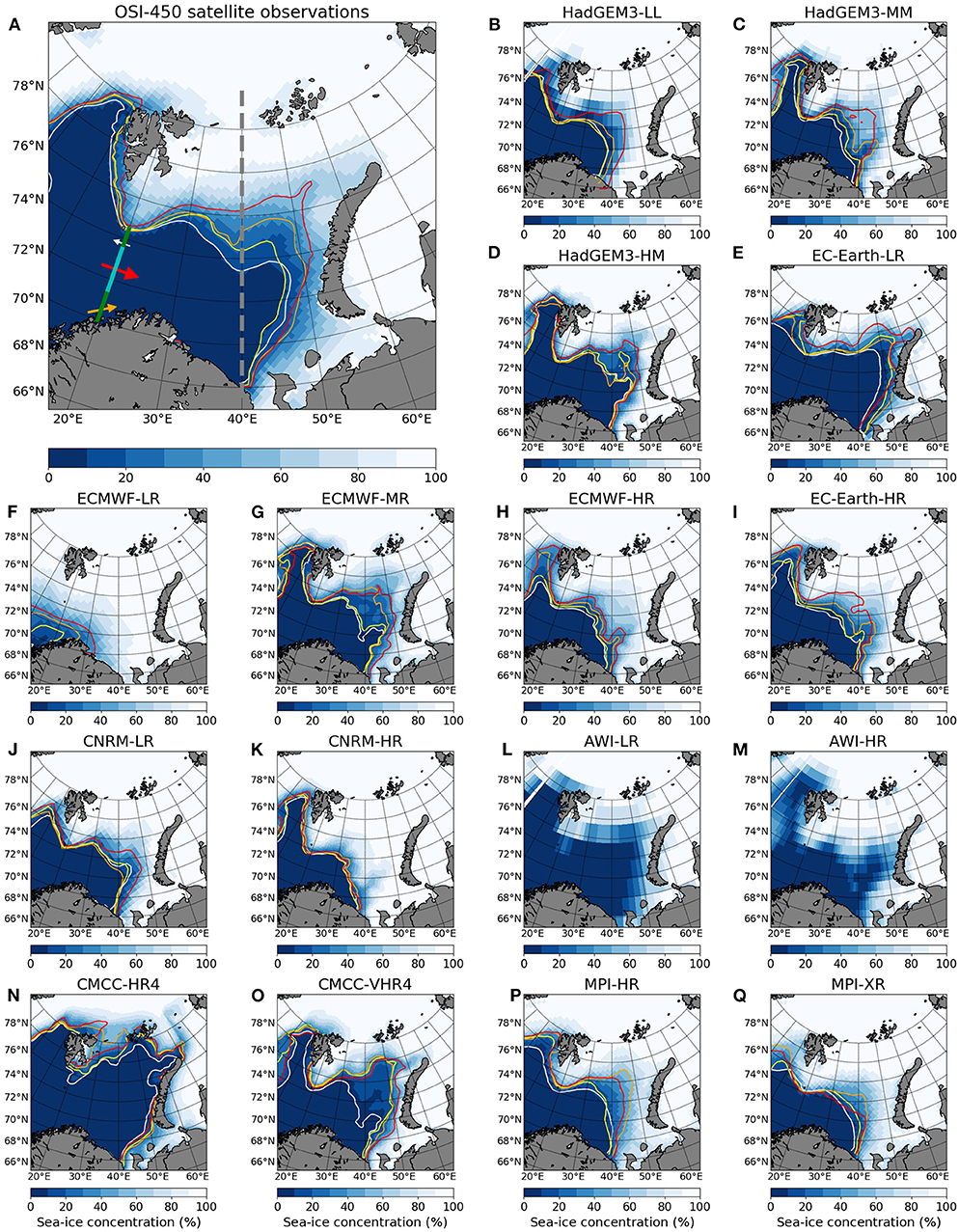
Figure 1. March sea-ice concentration in the Barents Sea from (A) OSI-450 satellite observations and (B–Q) HighResMIP hist-1950 model outputs, averaged over 1979–2014. The white, yellow, orange, and red contours show the mean March sea-ice edge (where sea-ice concentration is 15%) in 1980–1989, 1990–1999, 2000–2009, and 2010–2014, respectively. In (A), the green meridional transect (20°E, 70–74.5°N) shows the “large” Barents Sea Opening (BSO); the cyan meridional transect (20°E, 71.5–73.5°N) shows the “reduced” BSO (Atlantic Water contribution only); the dashed gray transect (40°E, 67.5–82°N) is the transect used in Figure 12; the red, orange, and white arrows represent the Atlantic Water inflow, Norwegian Coastal Current inflow, and Bear Island Trough outflow through the BSO, respectively.

The recent sea-ice area reduction in the Barents Sea is clearly linked to changes in the Atlantic Ocean heat transport (OHT). In particular, there has been a relatively recent increase in the Atlantic OHT due to both strengthening and warming of the Atlantic inflow (Arthun et al., 2012). Also, the Atlantic OHT has experienced large interannual and multi-decadal variability in the twentieth century, influencing the sea-ice cover in the Barents Sea (Muilwijk et al., 2018). On top of these OHT changes, large-scale changes in atmospheric circulation also influence sea-ice variability at time scales shorter than a year (Koenigk et al., 2009; Smedsrud et al., 2013). The main section of Atlantic OHT to the Barents Sea is the Barents Sea Opening, located in the western Barents Sea, between Bear Island and the northern extremity of Norway (Figure 1A). At the Barents Sea Opening, the Barents Sea receives 50 ± 22 TW of OHT from the Atlantic Water (mean over 1998–2016, update from Arthun et al., 2012). The observed OHT across the other parts of the Barents Sea Opening is only based on very short time scales and thus relatively uncertain. However, measurements show that the mean OHT to the Barents Sea from the Norwegian Coastal Current over 2007–2008 is 34 TW (Skagseth et al., 2011), and the mean OHT out of the Barents Sea through the Bear Island Trough over 2003–2005 is 12 TW (Skagseth, 2008). Thus, the net OHT to the Barents Sea through the Barents Sea Opening is about 70 TW (Smedsrud et al., 2010). This warm water inflow into the Barents Sea has the potential to melt sea ice and limit its growth there.

Linear extrapolation of the observed negative trend in sea-ice area suggests ice-free conditions in the Barents Sea all year round between 2023 and 2036 (Onarheim and Arthun, 2017), but this statistical projection is highly uncertain due to the presence of climate feedbacks and internal variability (Meier et al., 2007). Model simulations performed with the Community Earth System Model Large Ensemble (CESM-LE) using the Radiative Concentration Pathway (RCP) 8.5 provide a range of when each ensemble member becomes ice free (<80,000 km²) in the Barents Sea in winter for the first time between 2061 and 2088 (Onarheim and Arthun, 2017).

According to Onarheim and Arthun (2017), 72% of the negative trend in winter Barents sea-ice extent since 1979 is due to internal variability. In agreement with Onarheim and Arthun (2017), Li et al. (2017) find that the Atlantic OHT associated with regional internal variability has played a key role in the March Barents sea-ice extent decline, while the global warming signal appears not to be important, based on Coupled Model Intercomparison Project Phase 5 (CMIP5) models and recent observations. The Atlantic OHT inflow to the Barents Sea is a major source of internal variability in winter sea-ice variability, not only for the Barents Sea itself, but also for the whole Arctic based on CESM-LE model simulations, although the OHT-sea ice relationship weakens as the sea-ice cover decreases (Arthun et al., 2019). Koenigk and Brodeau (2014) show the leading role of OHT in the current Barents sea-ice reduction using the EC-Earth model. Muilwijk et al. (2019) use eight different ocean-only models and one fully coupled model, which have different resolutions, domains (both global and regional) and atmospheric forcing, and which are perturbed by adding the same wind anomaly over the Greenland Sea. They find that a stronger wind forcing leads to an increased OHT at the Barents Sea Opening and a reduced Barents sea-ice area. All these modeling studies point to a strong impact of Atlantic OHT on the Barents sea-ice changes, confirming the observed OHT-sea ice relationships (Arthun et al., 2012; Smedsrud et al., 2013).

Models participating in the High Resolution Model Intercomparison Project (HighResMIP; Haarsma et al., 2016) indicate that the horizontal resolution is important to correctly represent both Arctic sea ice and Atlantic OHT. In particular, the total Arctic sea-ice area and volume decrease and Atlantic OHT increases with increasing ocean resolution, suggesting a strong link between sea ice and OHT (Docquier et al., 2019). The suggested mechanism is that at higher ocean resolution, the boundary currents become stronger and warmer (Roberts et al., 2016; Grist et al., 2018), leading to larger OHT, which reduces the sea-ice cover. The strength of the sea ice—OHT link is not directly affected by model resolution, but the total Arctic sea-ice area and volume clearly decrease with increasing Atlantic OHT north of 60°N. Docquier et al. (2019) also show that the connection between sea-ice area/volume and OHT is the strongest in the Atlantic sector of the Arctic Ocean (i.e., Barents-Kara and Greenland-Iceland-Norway Seas).

In Docquier et al. (2019), the OHT is computed over the whole Atlantic Basin at three different latitudes (50, 60, and 70°N) and sea-ice area and volume are computed over the entire Arctic Ocean. In this paper, we further investigate the sea ice-OHT interactions in one of the most rapidly changing Arctic regions, namely the Barents Sea. Since sea ice is almost absent in summer in the Barents Sea, we focus on the winter season in this study. The two specific aims are: (1) to analyze how the Barents Sea ice and the OHT at the Barents Sea Opening behave in the seven HighResMIP models (16 different model configurations) used here; (2) to check the impact of model resolution on sea ice and OHT in the Barents Sea. In section 2, we provide a description of the models, reference products and diagnostics used. In section 3, we present the results of our analysis and discuss them. In section 4, we provide the conclusions of our study.

2. Methodology

2.1. Models

We use model outputs from the seven HighResMIP coupled atmosphere-ocean general circulation models (AOGCM) that are involved in the EU Horizon 2020 PRIMAVERA project (PRocess-based climate sIMulation: AdVances in high-resolution modeling and European climate Risk Assessment, https://www.primavera-h2020.eu/). HighResMIP is one of the CMIP6-endorsed Model Intercomparison Projects (MIPs), and its aim is to better understand the role of horizontal resolution in modeling the climate system (Haarsma et al., 2016). We focus on historical model simulations (“hist-1950”; 1950–2014) in order to evaluate models against observations and reanalyses, but we also make use of control runs (“control-1950”) in order to check the model drifts. The latter control runs use a fixed atmospheric forcing set at the year 1950 and have a duration of 100 years. In our analysis, we focus on the first 65 years of these control runs (1950–2014), in order to compare them to historical runs.

Each of the seven models has at least one “low” and one “high” resolution configuration, with two of these models having in addition an “intermediate” resolution configuration. Thus, 16 different model configurations are used here. A brief description of five out of the seven models [HadGEM3 (Roberts et al., 2019), ECMWF-IFS (Roberts et al., 2018b), AWI-CM (Sidorenko et al., 2015), CMCC-CM2 (Cherchi et al., 2019), and MPI-ESM (Gutjahr et al., 2019)] is given in section 2.1 of Docquier et al. (2019). The two other models (CNRM-CM6 and EC-Earth) are briefly described below. A summary of the atmosphere and ocean resolutions and model components of the 16 model configurations, as well as CMIP6 metadata, is given in Table 1. In five out of the seven models (HadGEM3, ECMWF-IFS, CNRM-CM6, EC-Earth, AWI-CM), both the atmosphere and ocean resolutions vary between configurations of the same model, while for the last two models (CMCC-CM2, MPI-ESM), only the atmosphere resolution varies. Note that the ECMWF-LR and ECMWF-HR model configurations both have six different ensemble members for historical runs, so that we present the ensemble means for these two model configurations in the figures and tables below (except in Figure 12, where only the first member is plotted).

TABLE 1

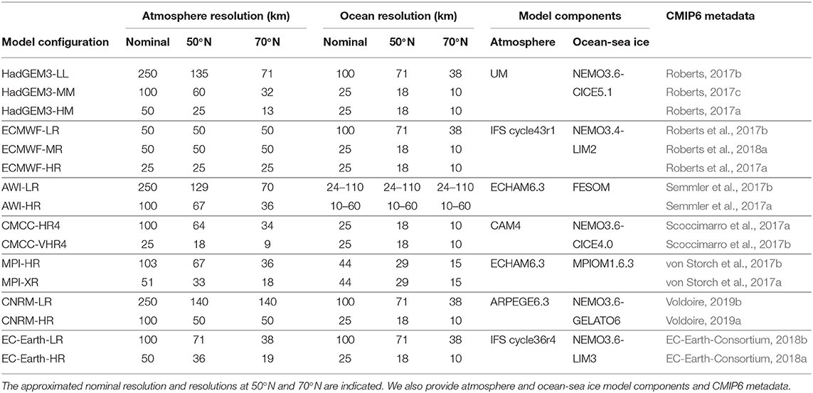
Table 1. Atmosphere and ocean resolutions (in km) of the model configurations used in this study.

CNRM-CM6-1, hereafter referred to as CNRM-CM6, is a fully coupled AOGCM jointly developed by CNRM (Centre National de Recherches Météorologiques) and CERFACS (Centre Européen de Recherche et de Formation Avancée en Calcul Scientifique) (Voldoire et al., 2019). It uses the version 6.3 of the global atmospheric model ARPEGE-Climat, which is a spectral model derived from the ARPEGE/IFS (Integrated Forecast System) numerical weather prediction model. The surface component SURFEX (Masson et al., 2013), which simulates surface fluxes at the Earth's surface, is coupled inline to ARPEGE-Climat. The ocean component of CNRM-CM6-1 is based on the version 3.6 of NEMO (Nucleus for European Modeling of the Ocean; Madec, 2016) and includes the version 6 of the GELATO sea-ice model (Voldoire et al., 2019). Two different configurations of CNRM-CM6 are used here. The first one, CNRM-LR, uses the TI127 atmosphere grid (nominal resolution of 250 km, i.e., 142 km at 50°N) and eORCA1 ocean grid (nominal resolution of 1°). The second configuration, CNRM-HR, uses the TI359 atmosphere grid (nominal resolution of 100 km, i.e., 50 km at 50°N) and eORCA025 ocean grid (nominal resolution of 0.25°).

EC-Earth3P, hereafter referred to as EC-Earth, is a coupled AOGCM developed by the EC-Earth Consortium (Haarsma et al., 2020). It is composed of the IFS atmosphere model, cycle 36r4, version 3.6 of the NEMO ocean model and version 3 of the Louvain-la-Neuve sea-Ice Model (LIM3; Rousset et al., 2015). Two different configurations of EC-Earth are used here. The first one, EC-Earth-LR, uses the TI255 atmosphere grid (nominal resolution of 100 km, i.e., 71 km at 50°N) and ORCA1 ocean grid (nominal resolution of 1°). The second configuration, EC-Earth-HR, uses the TI511 atmosphere grid (nominal resolution of 50 km, i.e., 36 km at 50°N) and ORCA025 ocean grid (nominal resolution of 0.25°).

A more detailed description of the different model biases and their possible origin can be found in Roberts et al. (2019) for HadGEM3, Roberts et al. (2018b) for ECMWF, Sidorenko et al. (2015) for AWI-CM, Cherchi et al. (2019) for CMCC-CM2, Gutjahr et al. (2019) for MPI-ESM, Voldoire et al. (2019) for CNRM-CM6, and Haarsma et al. (2020) for EC-Earth.

2.2. Reference Products

In order to evaluate our model results, different reference products (observations and reanalysis) are used for sea-ice concentration and OHT.

For sea-ice concentration, we use the second version of the global sea-ice concentration climate data record from the European Organization for the Exploitation of Meteorological Satellites (EUMETSAT) Ocean Sea Ice Satellite Application Facility (OSI SAF; Lavergne et al., 2019), named OSI-450. This product is a full reprocessing of sea-ice concentration, with improved algorithms and an upgraded processing chain, from 1979 to 2015. Sea-ice concentration is computed from the Scanning Multichannel Microwave Radiometer (SMMR, 1979–1987), Special Sensor Microwave/Imager (SSM/I, 1987–2008), and Special Sensor Microwave Imager Sounder (SSMIS, 2006–2015). The spatial resolution of OSI-450 is 25 km. This dataset compares well with independent estimates of sea-ice concentration both in regions with very high sea-ice concentration (3.5–4% accuracy) and in regions with very low sea-ice concentration (1.5–2%) (Lavergne et al., 2019). Errors in sea-ice concentration retrieval mainly come from surface emissivity variability over closed ice and weather-related effects at synoptic scale over open water (Lavergne et al., 2019). We compute the monthly mean concentration from daily data.

For the OHT at the Barents Sea Opening, we use the Atlantic Water OHT observational estimates (20°E, 71.5–73.5°N) derived from hydrographic data and current meter moorings (Ingvaldsen et al., 2004; Arthun et al., 2012). These data are provided by the Institute of Marine Research (IMR, Norway) and span from late 1997 to 2017. The main error sources of this dataset are the presence of mesoscale eddies and the extrapolation of each current meter to represent boxes with uniform velocity (Ingvaldsen et al., 2004). To characterize the large Barents Sea Opening section (between northern Norway and Bear Island), we also use OHT computed from the Ocean Reanalyses Intercomparison Project (ORA-IP; Uotila et al., 2019). In particular, we use the multi-model mean derived from eight reanalyses (C-GLORYS025v5, ECDA3, GLORYS2v4, GloSea5-GO5, MOVE-G2i, ORAP5, SODA3.3.1, UR025.4), spanning from 1993 to 2010. The mean error of the multi-model mean ORA-IP OHT (all Arctic straits) is 38 TW (Uotila et al., 2019) and comes from uncertainties in the model outputs of temperature and velocity. We also retrieve the ocean potential temperature from the ECMWF Ocean ReAnalysis System 4 (ORAS4; Balmaseda et al., 2013) for 1958 to 2014. This reanalysis is produced by combining the output of NEMO (ORCA1; 42 vertical levels) forced by atmospheric reanalysis fluxes and quality controlled ocean observations. This reanalysis shows an improvement in OHT compared to a control simulation without data assimilation, and errors mainly arise from the choice of the SST product, the model bias-correction scheme and the treatment of observations near the coast (Balmaseda et al., 2013).

2.3. Diagnostics

Ocean heat transport (OHT) across a section is computed as the spatial integral of the advective heat flux normal to the grid cells:

$\begin{array}{ll}\text{OHT}=\rho c_p{\displaystyle {\int }_A}\text{U}(T-T_{\text{ref}})dA,& (1)\end{array}$

where ρ is the water density (1,000 kg m⁻³), c_p is the specific seawater heat capacity (4,000 J kg⁻¹ K⁻¹), A is the surface area of the section, U is the ocean velocity perpendicular to the section, T is the ocean potential temperature, and T_ref is the reference temperature (set to 0°C). To define the section between two points, we follow the shortest broken line connecting the two relevant points, so that both the meridional and zonal components of ocean velocity are used. We also compute the horizontal ocean heat flux integrated over the vertical column (norm of meridional and zonal components) for each grid point of the model domains to analyze the spatial distribution of OHT.

The Barents Sea Opening is the western entrance to the Barents Sea between northern Norway and Bear Island. In our study, we use two meridional transects along 20°E to characterize the Barents Sea Opening (Figure 1A). The first transect (named “large Barents Sea Opening” in the following) corresponds to the section between 70°N (northern Norway) and 74.5°N (Bear Island). This transect takes into account all water inflows (i.e., Atlantic Water and Coastal Norwegian Current) and outflows (i.e., Bear Island Trough). We also choose to compute the OHT through a reduced transect (named “reduced Barents Sea Opening” in the following), i.e., between 71.5 and 73.5°N, corresponding to the Atlantic Water inflow only and excluding the coastal current, as monitoring of this transect has been more frequently than the large Barents Sea Opening transect (Arthun et al., 2012).

Sea-ice area is the product of sea-ice concentration and area of model grid cells summed over all grid cells for the region of interest. In this study, the Barents sea-ice area is computed between 70 and 81°N and between 15 and 60°E, as in Arthun et al. (2019).

3. Results and Discussion

Unless explicitly mentioned, we focus on the historical (hist-1950) model simulations in the following.

3.1. Sea-Ice Area

All models are able to reproduce a negative trend in the March Barents sea-ice area, except for CNRM-HR, which shows a small increase that is not significant (5 % level). However, the modeled trends are generally less negative than the observed trend of −91,700 ± 3,600 km² per decade (Figure 2 and Table 2). Furthermore, the trend in March Barents sea-ice area varies between −6,100 ± 1,400 km² per decade and −77,200 ± 3,000 km² per decade among the six members of ECMWF-LR, and between −7,400± 2,800 km² per decade and −22,600 ± 2,500 km² per decade among the six members of ECMWF-HR. Thus, there is a clear negative trend in all members of these two model configurations, but the role of internal variability is non-negligible, as shown by the relatively large spread in trends.

FIGURE 2

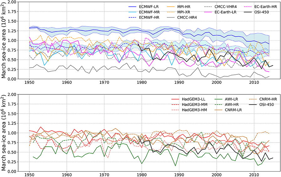
Figure 2. Time series of Barents sea-ice area in March over 1950–2014 using HighResMIP hist-1950 model outputs (split in two different panels for readability) and OSI-450 observations. The blue shadings of ECMWF-LR and ECMWF-HR represent the ensemble standard deviation (six members for each).

TABLE 2

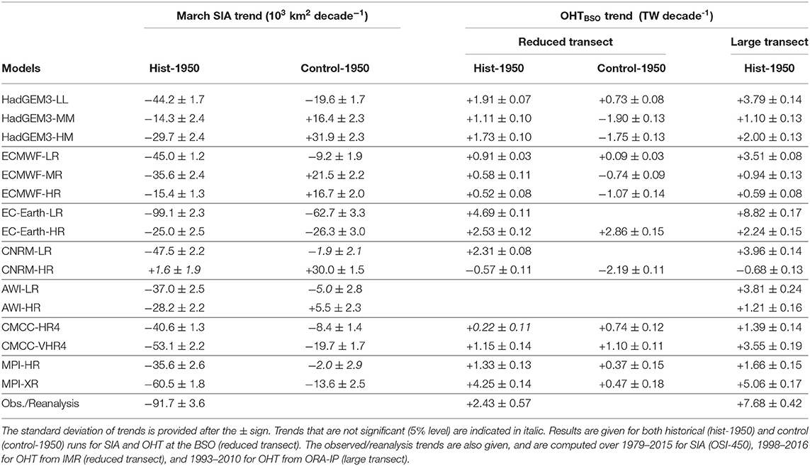
Table 2. Trends in March sea-ice area (SIA) in the Barents Sea and ocean heat transport (OHT) at the Barents Sea Opening (BSO; both reduced and large transects) for the different model configurations, computed for the record from 1950 to 2014.

The trends in March Barents sea-ice area of the control model simulations (fixed repeat year) are much less negative (either negative or positive) than the trends of the historical runs, except for EC-Earth-HR, which shows relatively similar trends in both control and historical simulations (Table 2). This confirms the robustness of the negative trends in sea-ice area in the historical runs.

The March Barents sea-ice area inter-model spread is relatively high, ranging between ~ 30,000 km² (CMCC-HR4 in 2013) and ~ 1.3 million km² (ECMWF-LR in 1988) during 1974–2014. For reference, the observed Barents sea-ice area in March starts from ~ 900,000 km² in 1979 and decreases to ~ 300,000 km² in 2014 (Figure 2).

The spatial distribution of the mean March sea-ice concentration in the Barents Sea for the different model configurations confirms that CMCC-HR4 (Figure 1N) and ECMWF-LR (Figure 1F) are both outliers compared to observations (Figure 1A), with too low and too high sea-ice area, respectively. All the other model configurations present a realistic spatial distribution of sea-ice concentration compared to observations (Figure 1).

A previous study using five out of the seven models used here showed that a higher ocean resolution leads to lower total Arctic sea-ice area during all months, except for a slight increase in sea-ice area for AWI-CM in winter (Docquier et al., 2019). Adding the two remaining models (EC-Earth and CNRM-CM6) confirms this impact of ocean resolution on the total Arctic sea-ice area (Table 3). The decrease in total Arctic sea-ice area is associated with larger poleward Atlantic OHT at higher ocean resolution, which is driven by stronger and warmer boundary currents (Docquier et al., 2019). However, when focusing on the Barents Sea, the impact of ocean resolution on March sea-ice area is not as clear cut, with a decrease in area for HadGEM3 and ECMWF-IFS, and an increase in area for EC-Earth, CNRM-CM6 and AWI-CM with higher ocean resolution (Figure 2 and Table 3). The control simulations show similar results regarding the impact of ocean resolution on the March Barents sea-ice area. Thus, no systematic response of the Barents sea-ice area with resolution is found here.

TABLE 3

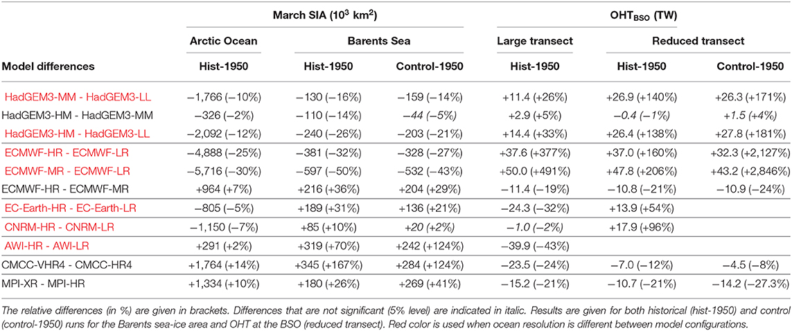
Table 3. Mean differences in March sea-ice area (SIA; both pan-Arctic and Barents Sea) and ocean heat transport (OHT) at the Barents Sea Opening (BSO; both large and reduced transects) between the different configurations of each model, averaged for the record from 1950 to 2014.

An increase in atmosphere resolution leads to a decrease in both pan-Arctic and Barents sea-ice area in March for HadGEM3, and an increase in both quantities for ECMWF-IFS, CMCC-CM2, and MPI-ESM (Figure 2 and Table 3). As for ocean resolution, the impact of atmosphere resolution on the March Barents sea-ice area in control runs is comparable to historical runs (Table 3).

The contrasting behavior between the impact of ocean resolution on the total Arctic sea-ice area (Docquier et al., 2019) and its impact on the Barents sea-ice area (this study) reveals that it is important to inspect specific Arctic regions separately. In the following, we will show that the OHT at the Barents Sea Opening is a possible reason for this difference.

3.2. Ocean Heat Transport (OHT)

As mentioned in section 2.3, the OHT at the Barents Sea Opening is computed through two different transects, i.e., a reduced transect taking into account the Atlantic Water only and a large Barents Sea Opening transect between northern Norway and Bear Island. We will analyze the model results in both transects separately in the following. We will also investigate the spatial distribution of ocean heat flux in the Barents Sea.

3.2.1. Reduced Barents Sea Opening Transect

Considering the reduced transect, all models exhibit a positive trend in annual mean OHT at the Barents Sea Opening over 1950–2014, except for CNRM-HR, which shows a small decrease (Figure 3 and Table 2). Despite the relatively short observational record (1998–2016) and high interannual variability, this result is consistent with the observed positive trend in OHT (+2.43 ± 0.57 TW decade⁻¹). Furthermore, the trend in OHT at the Barents Sea Opening varies between +0.11 ± 0.02 TW per decade and +2.09 ± 0.07 TW per decade among the six members of ECMWF-LR, and between −0.19± 0.17 TW per decade and +1.13 ± 0.11 TW per decade among the six members of ECMWF-HR. This indicates that there is a positive trend in all members of these two model configurations (except for one ECMWF-HR member), but the role of internal variability is non-negligible, as shown by the relatively large spread in trends.

FIGURE 3

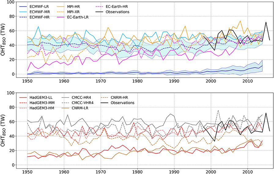
Figure 3. Time series of annual mean ocean heat transport (OHT) at the Barents Sea Opening (BSO, reduced transect, 20°E, 71.5–73.5°N) over 1950–2014 using HighResMIP hist-1950 model outputs (split in two different panels for readability) and IMR observations. The blue shadings of ECMWF-LR and ECMWF-HR represent the ensemble standard deviation (six members for each).

For HadGEM3, ECMWF-IFS and MPI-ESM, the trends in annual mean OHT at the Barents Sea Opening of the control model simulations are much less positive (either negative or slightly positive) than the trends of the historical runs (Table 2). This confirms the robustness of the positive trends in OHT in the historical runs of these models. However, the trends in OHT are of similar order in both control and historical simulations for EC-Earth-HR and CMCC-VHR4, and even larger in control runs for CMCC-HR4, which prevents to make robust conclusions regarding the historical trends in OHT for these three model configurations (Table 2).

The inter-model spread in annual mean OHT at the Barents Sea Opening is relatively high, with values ranging from ~ 0 (ECMWF-LR in 1950–1980) to ~ 70 TW (CMCC-HR4, CMCC-VHR4, and MPI-HR in the end of the record). For reference, the observed OHT at the Barents Sea Opening varies between ~ 35 and ~ 70 TW (Figure 3), with a seasonal cycle showing a minimum in April and a maximum in January (Figure 4). The low-resolution configurations of ECMWF-IFS, HadGEM3 and CNRM-CM6 clearly fall below the uncertainty range of OHT observations, while the two CMCC-CM2 configurations are above the observed uncertainty range in October-December (Figure 4).

FIGURE 4

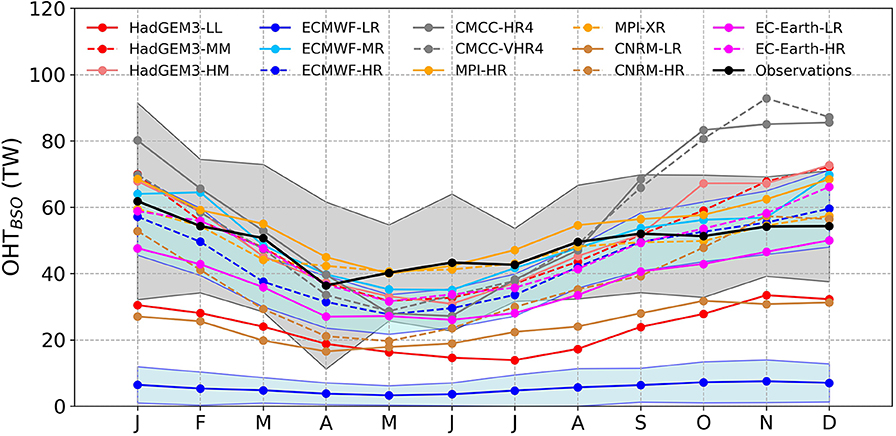
Figure 4. Seasonal cycle of ocean heat transport (OHT) at the Barents Sea Opening (BSO, reduced transect, 20°E, 71.5–73.5°N) averaged over 1998–2014 using HighResMIP hist-1950 model outputs and IMR observations. The blue shadings of ECMWF-LR and ECMWF-HR represent the ensemble standard deviation (six members for each). The gray shading of observations represents the temporal standard deviation.

A remarkable feature is that an increased ocean resolution results in higher OHT at the Barents Sea Opening for all models, in much better agreement with observations compared to lower resolution (Figures 3, 4 and Table 3). This sensitivity to model resolution is also found in the control runs (Table 3). Using five out of the seven models used here, Docquier et al. (2019) find that the mean poleward Atlantic OHT increases with higher ocean resolution, in agreement with results found here for the OHT at the Barents Sea Opening (reduced transect). A potential reason for an increased OHT at higher ocean resolution is that the boundary currents get stronger and warmer at higher ocean resolution, as found in Roberts et al. (2016), Grist et al. (2018), and Docquier et al. (2019).

A higher ocean resolution also leads to a lower trend in annual mean OHT at the Barents Sea Opening (Figure 3 and Table 2). This correlates well with less negative trends in March sea-ice area in the Barents Sea with higher ocean resolution (Figure 2 and Table 2).

3.2.2. Large Barents Sea Opening Transect

If we consider the large Barents Sea Opening transect between northern Norway and Bear Island, the OHT is higher compared to the OHT through the reduced transect, due to the additional contribution from the Norwegian Coastal Current (compare Figure 5 to Figure 3, and Figure 6 to Figure 4).

FIGURE 5

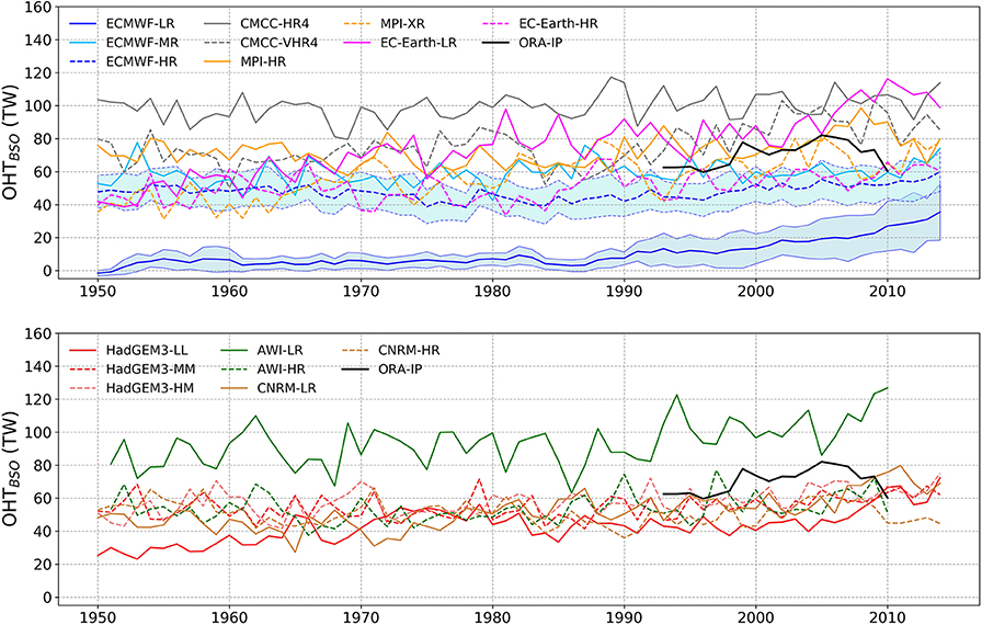
Figure 5. Time series of annual mean ocean heat transport (OHT) at the Barents Sea Opening (BSO, large transect, 20°E, 70–74.5°N) over 1950–2014 using HighResMIP hist-1950 model outputs (split in two different panels for readability) and ORA-IP reanalyses. The blue shadings of ECMWF-LR and ECMWF-HR represent the ensemble standard deviation (six members for each).

FIGURE 6

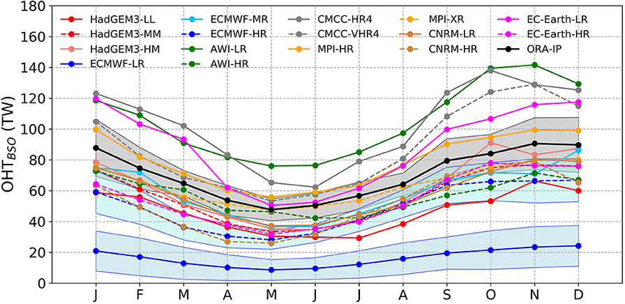
Figure 6. Seasonal cycle of ocean heat transport (OHT) at the Barents Sea Opening (BSO, large transect, 20°E, 70–74.5°N) averaged over 1993–2010 using HighResMIP hist-1950 model outputs and ORA-IP reanalyses. The blue shadings of ECMWF-LR and ECMWF-HR represent the ensemble standard deviation (six members for each). The gray shading of reanalyses represents the temporal standard deviation.

As for the reduced transect, all models show a positive trend in annual mean OHT at the Barents Sea Opening for the large transect, ranging between 0.59 and 8.82 TW decade⁻¹, except for CNRM-HR (Figure 5 and Table 2). As no observational dataset is available for the large Barents Sea Opening transect, we make use of ORA-IP reanalyses. Despite the very limited temporal record available for ORA-IP (1993–2010), this dataset also produces a positive trend in OHT at the Barents Sea Opening (+7.68 ± 0.42 TW decade⁻¹), strengthening the HighResMIP results. This is also in agreement with Muilwijk et al. (2018), who run the global ocean model NorESM20CR forced by atmospheric reanalysis over the full 20th century. The latter find an increase in OHT at the Barents Sea Opening of about 30 TW in 100 years, so about 3 TW decade⁻¹, which is in the middle range of our model estimates.

Excluding the ECMWF-LR configuration (which has a very low OHT), the ensemble mean ORA-IP OHT lies in the middle of the HighResMIP OHT spread, with a minimum of ~ 50 TW in May and a maximum of ~ 90 TW in November-January (Figure 6), in agreement with Smedsrud et al. (2010). The MPI-HR configuration is the closest to ORA-IP in terms of mean OHT (average over 1993–2010), while most models fall outside of the uncertainty range of ORA-IP (Figure 6).

A higher ocean resolution leads to higher OHT at the Barents Sea Opening for ECMWF-IFS and HadGEM3, in better agreement with ORA-IP reanalyses, lower OHT for EC-Earth and AWI-CM, and slightly lower OHT (but not significantly) for CNRM-CM6 (Figures 5, 6 and Table 3). A higher atmosphere resolution leads to slightly higher OHT for HadGEM3, and lower OHT for ECMWF-IFS, CMCC-CM2 and MPI-ESM (Figures 5, 6 and Table 3). Thus, no systematic response of the OHT at the Barents Sea Opening (large transect) with resolution is found.

However, note that these results are perfectly anticorrelated with the impact of resolution on March Barents sea-ice area (Table 3): when the Barents sea-ice area decreases (increases, respectively) with higher atmosphere/ocean resolution, the OHT at the Barents Sea Opening increases (decreases, respectively). This finding confirms the link between OHT and sea-ice area in the Barents Sea, in agreement with previous studies (Arthun and Schrum, 2010; Sando et al., 2014). In section 3.3, we will further investigate the links between OHT and sea-ice area in the Barents Sea.

Finally, as for the reduced transect, a higher ocean resolution results in a lower trend in annual mean OHT at the Barents Sea Opening (Figure 5 and Table 2). Again, this correlates well with less negative trends in March sea-ice area in the Barents Sea with higher ocean resolution (Figure 2 and Table 2).

3.2.3. Ocean Heat Flux

As found in section 3.2.2, the OHT at the Barents Sea Opening does not necessarily increase with higher ocean resolution when considering the large transect, while it does in all models for the reduced transect. In order to investigate the reason behind this finding, we look at the spatial distribution of the horizontal ocean heat flux in the Barents Sea (Figure 7).

FIGURE 7

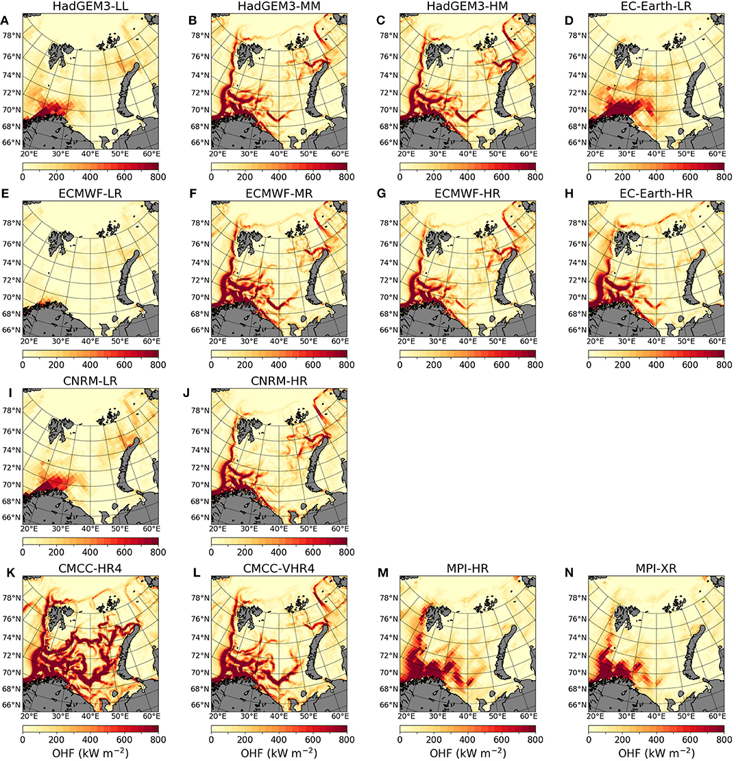
Figure 7. Mean horizontal ocean heat flux (OHF) in the Barents Sea from HighResMIP hist-1950 model outputs, averaged over 1950–2014.

The low-resolution configurations of HadGEM3, EC-Earth and CNRM-CM6, which all have an ocean resolution of 1°, present a very similar spatial distribution of ocean heat flux in the vicinity of the Barents Sea Opening (Figures 7A,D,I). They produce a “patch” of stronger ocean heat flux in a box between 70°N to 72–73°N and 20°E to 30°E. As the resolution is too coarse to accurately distinguish the Atlantic Water from the Norwegian Coastal Current, there is only one single water inflow to the Barents Sea in the vicinity of the Barents Sea Opening in these model configurations.

The high-resolution configurations of HadGEM3, ECMWF-IFS, EC-Earth, and CNRM-CM6, as well as CMCC-VHR4, which all have an ocean resolution of 0.25°, are also very similar in terms of the ocean heat flux spatial distribution (Figures 7B,C,F–H,J,L). In these configurations, we can clearly distinguish the two main water inflows to the Barents Sea through the Barents Sea Opening, i.e., the Atlantic Water and Norwegian Coastal Current. Also, the water inflow through Fram Strait is clearly distinguishable in these high-resolution configurations. The more detailed path of surface circulation in the Barents Sea at higher ocean resolution was already found in Docquier et al. (2019).

The two MPI-ESM configurations, both having an intermediate ocean resolution (0.4°), have a mixed behavior in the sense that ocean currents are better defined than at 1°, but are far from being as detailed as at 0.25° (Figures 7M,N).

Ocean heat flux in the Barents Sea in ECMWF-LR and CMCC-HR4 deviate strongly from the other model configurations; ECMWF-LR has a very weak ocean heat flux (Figure 7E), while CMCC-HR4 has a very strong ocean heat flux (Figure 7K), compared to other model configurations. The too low ocean heat flux of ECMWF-LR is linked to the strong negative bias in North Atlantic SST, which is improved at higher ocean resolution (Roberts et al., 2018b), and also to the absence of deep water formation, which leads to weak Atlantic Meridional Overturning Circulation (AMOC) in this model (Roberts et al., under review). It is interesting to note that ECMWF-LR and CMCC-HR4 also have relatively high and low (respectively) March sea-ice concentration in the Barents Sea (section 3.1; Figures 1F,N).

In summary, the underrepresentation of the Atlantic Water and Norwegian Coastal Current inflows at the Barents Sea Opening in low-resolution configurations is a possible reason for the different impact of ocean resolution on OHT at the Barents Sea Opening between the reduced and large transects (Figure 7). For example, the OHT at the Barents Sea Opening (large transect) decreases with higher ocean resolution for EC-Earth and CNRM-CM6 (Figure 6 and Table 3), while it increases with higher ocean resolution when using the reduced transect for these two models (Figure 4 and Table 3). The higher OHT at the Barents Sea Opening (large transect) with lower ocean resolution for these two models is probably linked to the relatively high ocean heat flux in the vicinity of northern Norway at lower resolution (Figures 7D,I), compared to the respective high-resolution configurations (Figures 7H,J).

3.3. Relationships Between Sea-Ice Area and Ocean Heat Transport (OHT)

Linking the results in sections 3.1 and 3.2, we find evidence for a potential link between the March Barents sea-ice area and OHT at the Barents Sea Opening in HighResMIP model outputs. In particular, the negative trend in March Barents sea-ice area over the historical record goes in hand with the positive trend in annual mean OHT at the Barents Sea Opening shown by 15 out of the 16 model configurations (Table 2). The only model configuration presenting a slightly positive trend in sea-ice area (CNRM-HR) has a negative trend in annual mean OHT. Furthermore, a higher ocean resolution leads to a lower trend in annual mean OHT at the Barents Sea Opening and to a less negative trend in March Barents sea-ice area (Table 2). Also, we find that when the March Barents sea-ice area decreases (increases, respectively) with higher resolution for a given model configuration, the OHT at the Barents Sea Opening increases (decreases, respectively) for that configuration (Table 3). In the following, we will investigate more deeply the relationships between the March Barents sea-ice area and annual mean OHT at the Barents Sea Opening (large transect) using scatter plots and vertical profiles of ocean temperature.

3.3.1. Scatter Plots

The models with higher mean OHT at the Barents Sea Opening (large transect) have lower mean March Barents sea-ice area (R = −0.94; Figure 8A). This result is in agreement with Mahlstein and Knutti (2011), who focus on the relationship between northward Atlantic OHT and Arctic sea-ice extent in CMIP3 models, and Muilwijk et al. (2019), who find such a link using nine different climate models. The trends in OHT at the Barents Sea Opening and March Barents sea-ice area are weakly correlated to the mean OHT at the Barents Sea Opening (R = 0.17 and −0.26, respectively; Figures 8B,C). However, when removing ECMWF-LR (which has too much ice compared to observations and other models), CMCC-HR4 and AWI-LR (both have too low sea-ice area) from the model list, the trend in OHT at the Barents Sea Opening significantly increases with the mean OHT (R = 0.53) and the trend in March Barents sea-ice area significantly decreases with the mean OHT (R = −0.64). These results suggest that having a correct mean OHT at the Barents Sea Opening is important to correctly model changes in OHT at the Barents Sea Opening and sea-ice area in the Barents Sea.

FIGURE 8

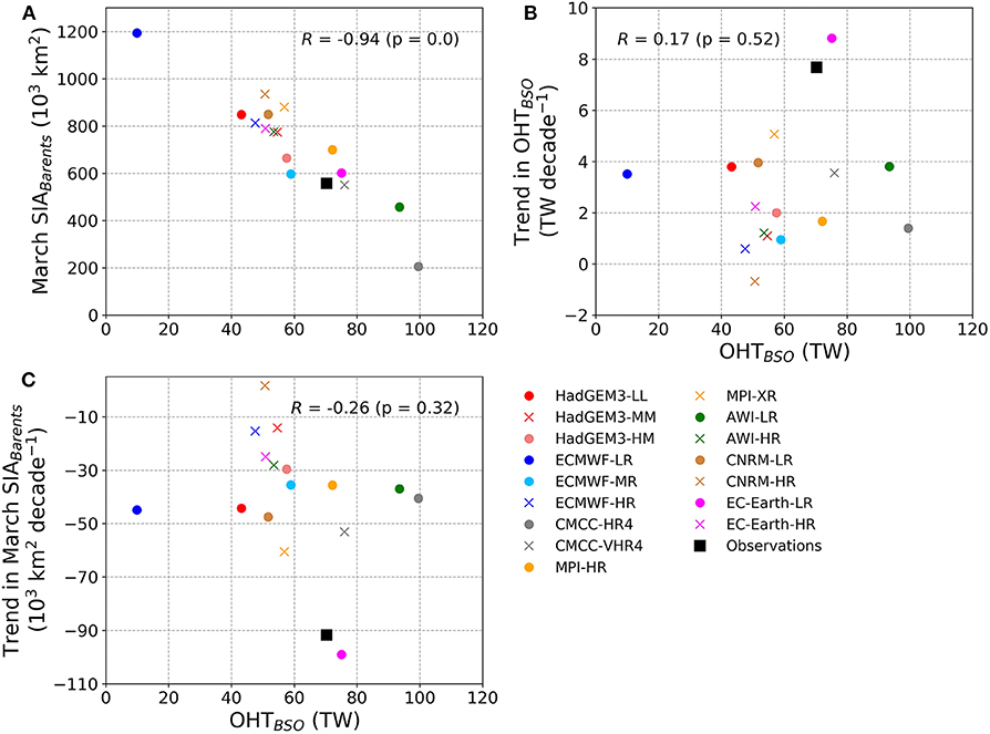
Figure 8. Scatter plots of (A) mean March Barents sea-ice area (SIA_Barents), (B) trend in ocean heat transport (OHT) at the Barents Sea Opening (BSO, large transect), and (C) trend in March Barents sea-ice area against mean OHT at the BSO (large transect) for all HighResMIP hist-1950 model outputs (averaged over 1950–2014) and observations/reanalysis. Observed sea-ice area is averaged over 1979–2014 and ORA-IP reanalysis for OHT is averaged over 1993–2010. Correlation coefficients R (with their p-value) are indicated in the upper left/right corner of each panel.

To further investigate the links between sea-ice area and OHT, we regress the detrended March Barents sea-ice area against the detrended mean OHT at the Barents Sea Opening (large transect) over the full record (1950–2014) for each model configuration. The use of detrended variables allows to isolate the relationships associated with interannual variability. We use both annual mean and five-year running mean for the two variables. When using annual mean, we look at lead-lag correlations between OHT and sea-ice area, with OHT leading sea-ice area by 1, 2, and 3 years. Thus, in total, there are five different combinations: (1) annual mean without lag, (2) 5-year running mean, (3) annual mean OHT leading sea-ice area by 1 year, (4) by 2 years, and (5) by 3 years.

Figure 9 illustrates the results when regressing March Barents sea-ice area against annual mean OHT with OHT leading sea-ice area by 1 year (the case for which correlations are highest). A significant anticorrelation (5 % level) exists for all model configurations, except for CMCC-HR4 (but the correlation is still negative). The sensitivity is highest for ECMWF-LR, with a sea-ice loss of 13,723 ± 916 km² per TW of OHT (Figure 9E), and lowest for CMCC-HR4, with a sea-ice loss of 1,820 ± 1,188 km² per TW of OHT (Figure 9M). The correlation between observed March sea-ice area and annual mean OHT from ORA-IP reanalysis is negative (Figure 9Q) but not significant (5 % level), due to the too short time record (1993–2010). The observed/reanalysis sensitivity lies in the upper range of model configurations, with a sea-ice loss of 9,473 ± 5,488 km² per TW of OHT (Figure 9Q).

FIGURE 9

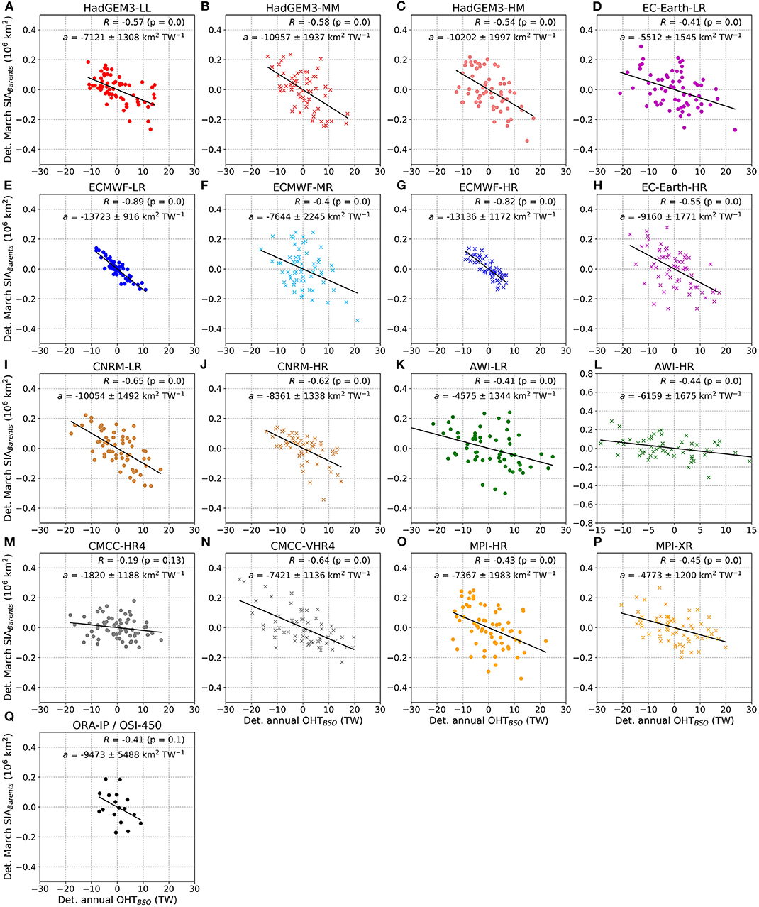
Figure 9. Scatter plots of detrended mean March Barents sea-ice area (SIA_Barents) against detrended annual mean ocean heat transport (OHT) at the Barents Sea Opening (large OHT_BSO transect) in (A–P) HighResMIP hist-1950 model outputs and (Q) reanalysis/observations, with OHT leading SIA by 1 year. All yearly values between 1950 and 2014 (1993–2010 for ORA-IP reanalyses/OSI-450 observations) are plotted. Correlation coefficients R and regression slopes a (with their respective p-value and standard deviation) are indicated in the upper right corner of each panel.

The regression slopes between detrended March Barents sea-ice area and detrended OHT at the Barents Sea Opening are shown in Figure 10 for the five different combinations: (1) annual mean (Figure 10A), (2) 5-year running mean (Figure 10B), (3) annual mean OHT leading March sea-ice area by 1 year (Figure 10C), (4) annual mean OHT leading March sea-ice area by 2 years (Figure 10D), and (5) annual mean OHT leading March sea-ice area by 3 years (Figure 10E). These results display the clear anticorrelation between March sea-ice area and annual mean OHT for all model configurations when OHT leads sea-ice area by 1 year (Figure 10C), as previously mentioned (Figure 9). Without lagged correlation, the anticorrelation is still present in most model configurations, although generally weaker (Figures 10A,B). Note that the observed correlation becomes positive (but not significant at the 5 % level) when using the 5-year running mean (Figure 10B), but the temporal reanalysis record is very short (1993–2010). When OHT leads sea-ice area by 2 or 3 years, results are not as clear cut, although there are more model configurations with a negative correlation than configurations with a positive correlation (Figures 10D,E). This suggests that the annual mean OHT at the Barents Sea Opening of a given year is crucial in defining the area of sea ice in the Barents Sea the year after, in agreement with previous studies (Arthun et al., 2012; Koenigk and Brodeau, 2014; Sando et al., 2014; Auclair and Tremblay, 2018; Muilwijk et al., 2019).

FIGURE 10

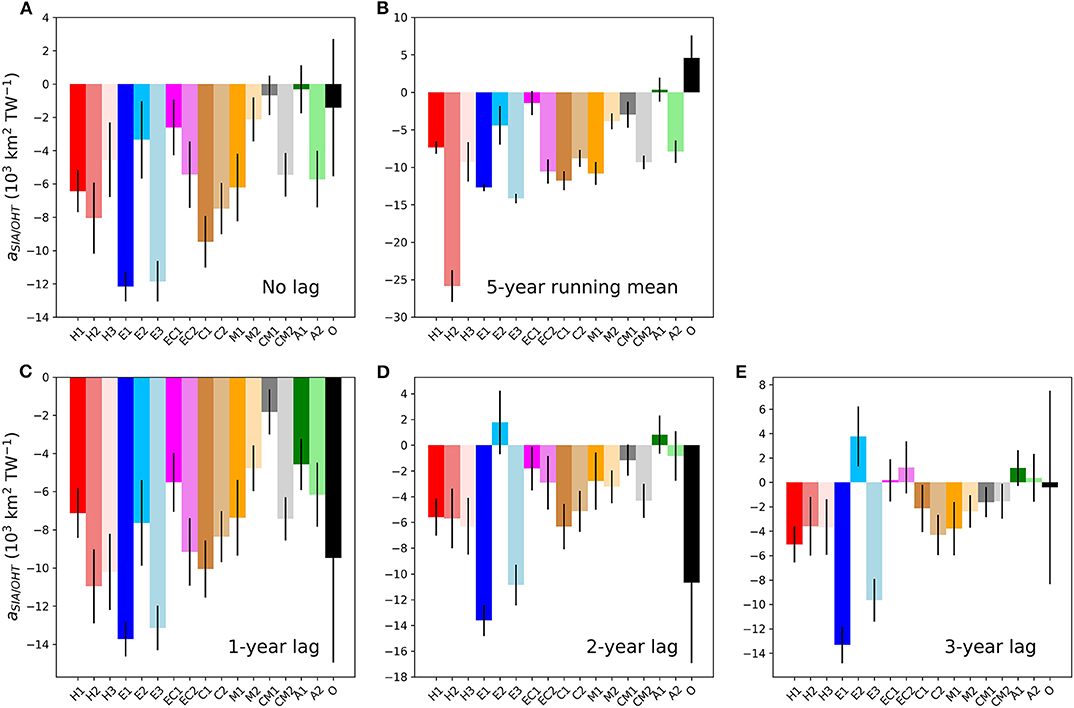
Figure 10. (A) Regression slopes (a_SIA/OHT) between detrended March Barents sea-ice area and detrended annual mean ocean heat transport (OHT) at the Barents Sea Opening (BSO, large transect) for all HighResMIP hist-1950 model outputs (1950–2014) and observations/renalysis (1993–2010). (B) Same as (A) with 5-year running mean instead of annual mean. (C–E) Same as (A) with OHT leading sea-ice area by (C) 1 year, (D) 2 years, (E) 3 years. The X axis shows the 16 model configurations used (H1 = HadGEM3-LL, H2 = HadGEM3-MM, H3 = HadGEM3-HM, E1 = ECMWF-LR, E2 = ECMWF-MR, E3 = ECMWF-HR, EC1 = EC-Earth-LR, EC2 = EC-Earth-HR, C1 = CNRM-LR, C2 = CNRM-HR, M1 = MPI-HR, M2 = MPI-XR, CM1 = CMCC-HR4, CM2 = CMCC-VHR4, A1 = AWI-LR, A2 = AWI-HR) and observations/reanalysis (O). The black line on top of each bar indicates the standard deviation of the regression slopes.

It is interesting to note that the model configurations presenting the least negative regression slopes (CMCC-HR4 and AWI-LR; Figures 10A–C) are the ones with the lowest mean March Barents sea-ice area and highest annual mean OHT at the Barents Sea Opening (Figure 8A). On the contrary, ECMWF-LR and ECMWF-HR have highly negative sea-ice area—OHT anticorrelations (Figures 10A–C), high March Barents sea-ice area and low OHT at the Barents Sea Opening (Figure 8A). Thus, the sensitivity of March Barents sea-ice area to annual mean OHT at the Barents Sea Opening is higher for models with stronger mean Barents sea-ice area (R = −0.67; Figure 11A) and lower annual mean OHT (R = −0.76; Figure 11B). This indicates that properly simulating the mean OHT at the Barents Sea Opening is crucial in order to derive the required sensitivity of Barents sea-ice area to OHT.

FIGURE 11

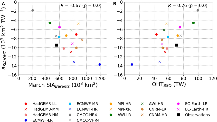
Figure 11. Scatter plots of regression slopes (a_SIA/OHT) between detrended March Barents sea-ice area (SIA_Barents) and detrended annual mean ocean heat transport (OHT) at the Barents Sea Opening (BSO, large transect; OHT leads SIA by 1 year) against (A) mean March Barents sea-ice area, and (B) annual mean OHT at the Barents Sea Opening (large transect) for all HighResMIP hist-1950 model outputs (averaged over 1950–2014) and observations/reanalysis. Correlation coefficients R (with their p-value) are indicated in the upper right corner of each panel.

3.3.2. Vertical Profiles

The vertically-integrated OHT does not provide information on the vertical distribution of the inflowing warm water. However, the warm water masses at the ocean surface have a large impact on sea ice in the Barents Sea. Thus, in the following, we analyze vertical profiles of mean ocean potential temperature and corresponding longitudinal profiles of March sea-ice concentration in the central Barents Sea (along 40°E, between 67.5° and 82°N) to check the connection between ocean temperature and sea-ice edge. For this analysis, we focus on the record from 1983 to 2014 (Figure 12), but using the record from 1950 to 1982 also provides similar results with generally lower ocean temperature (not shown). We focus here on the ocean temperature due to its strong connection to the growth and melt of sea ice, but we recognize that the ocean dynamics also constitutes an important component of OHT (Muilwijk et al., 2018; Asbjornsen et al., 2019), thus indirectly leading to sea-ice changes.

FIGURE 12

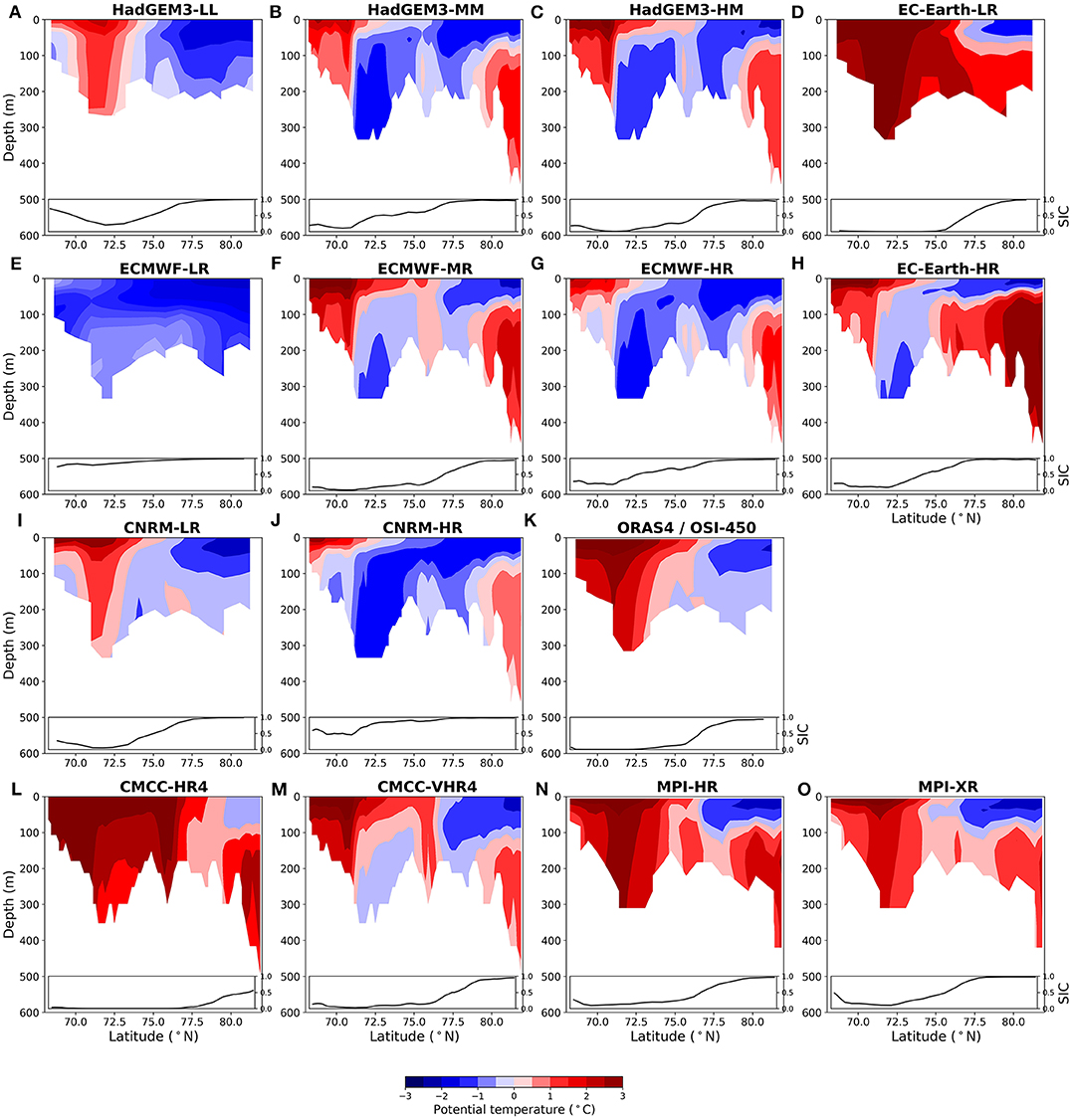
Figure 12. Vertical profiles of mean ocean potential temperature along a meridional transect located in the central Barents Sea (40°E, 67.5–82°N). The longitudinal profile of mean March sea-ice concentration (SIC, no unit) at 40°E is also plotted below each vertical profile. Results from (A–J,L–O) HighResMIP hist-1950 model outputs and (K) ORAS4 reanalysis (OSI-450 satellite observations for sea-ice concentration), averaged over 1983–2014. Only the first member is plotted for ECMWF-LR and ECMWF-HR.

In all models, the warm water advances northward to the sea-ice edge where it is strongly cooled (Figure 12), except for ECMWF-LR, which stays too cold and with almost 100% sea-ice concentration (Figure 12E). During the winter (which we show here), this warm water is cooled by heat release to the atmosphere, sinks down and forms the warm intermediate Atlantic Water layer (Koenigk and Brodeau, 2014). In agreement with Koenigk and Brodeau (2014), who used a previous version of the EC-Earth model with the T159 grid in the atmosphere and ORCA1 in the ocean, we also find such a behavior for the majority of model configurations (Figure 12). The high-resolution model configurations perform better to capture this phenomenon, although the degree of warming greatly varies among models (Figure 12). This could be due to the more detailed bathymetry in high-resolution model configurations.

For HadGEM3 and ECMWF-IFS, increasing the ocean resolution clearly leads to higher ocean temperatures, especially south of 70°N and north of 80°N (compare Figure 12A to Figures 12B,C, and Figure 12E to Figures 12F,G). This enhances the eastward and northward retreats of the Barents sea-ice edge (sea-ice concentration lower than 15%) in the high-resolution configurations (Figures 1, 12). This is in line with higher OHT at the Barents Sea Opening (section 3.2) and lower March Barents sea-ice area (section 3.1) with enhanced ocean resolution for these two models (Table 3). However, the region between ~ 71° and ~ 73°N is warmer in the low-resolution configurations of HadGEM3 and ECMWF-IFS, especially below 100 m depth. This translates into relatively low sea-ice concentration (<50%) in that region for HadGEM3-LL.

Increasing the ocean resolution in EC-Earth and CNRM-CM6 generally leads to lower ocean temperatures, especially in the region between ~ 71° and ~ 73°N (compare Figure 12D to Figure 12H, and Figure 12I to Figure 12J). This feature is more pronounced for EC-Earth and is probably linked to the higher OHT at the Barents Sea Opening (large transect; Figure 6) and higher ocean heat flux (Figure 7), leading to more ocean heat transported eastward into the Barents Sea at lower ocean resolution. The lower ocean temperatures at higher ocean resolution in EC-Earth and CNRM-CM6 lead to an ice edge that is more advanced further west and south in high-resolution configurations (Figures 1, 12). Again, these findings are in line with lower OHT at the Barents Sea Opening (section 3.2) and higher March Barents sea-ice area (section 3.1) with increased ocean resolution for these two models (Table 3).

An increase in atmosphere resolution leads to lower ocean temperatures for ECMWF-IFS (compare Figure 12F to Figure 12G), CMCC-CM2 (compare Figure 12L to Figure 12M) and MPI-ESM (compare Figure 12N to Figure 12O), and slightly larger ocean temperatures for HadGEM3 (Figure 12B to Figure 12C). Accordingly, there is generally an advance further west and south in the Barents sea-ice edge in the first three model configurations and a retreat further east and north for HadGEM3 (Figures 1, 12). These findings are in line with lower OHT at the Barents Sea Opening and higher March Barents sea-ice area with higher atmosphere resolution for ECMWF-IFS, CMCC-CM2, and MPI-ESM, and higher OHT at the Barents Sea Opening and lower Barents sea-ice area with enhanced atmosphere resolution for HadGEM3 (sections 3.1, 3.2, Table 3).

This analysis also confirms that ECMWF-LR and CMCC-HR4 are two outliers, with relatively cold temperature and high sea-ice concentration for ECMWF-LR, and relatively warm temperature and low sea-ice concentration for CMCC-HR4, compared to other model configurations and the ORAS4 reanalysis (Figure 12). This finding agrees with lower/higher OHT at the Barents Sea Opening for ECMWF-LR/CMCC-HR4 (respectively), compared to other model configurations (Figure 4).

In summary, the analysis of vertical profiles of ocean temperature shows the strong connection between ocean temperature and the presence of sea ice in the Barents Sea, with a more retreated/advanced ice edge with higher/lower ocean temperature, respectively. Also, there is no systematic impact of model resolution on the ocean temperature, but the strong cooling at the sea-ice edge and further formation of warm intermediate Atlantic Water is better depicted at higher ocean resolution.

4. Conclusions

This study provides the first detailed multi-model comparison on the impact of model resolution on the sea-ice area and ocean heat transport (OHT) in the Barents Sea. It also constitutes one of the few detailed analyses (with e.g., Li et al., 2017; Muilwijk et al., 2019) on the relationship between Barents Sea ice and OHT in a multi-model framework. We use seven AOGCMs with different horizontal resolutions and participating to the HighResMIP experiments (1950–2014). The following key results emerge from our analysis:

1. The impact of increased ocean and atmosphere resolutions on the March Barents sea-ice area depends on the model used (section 3.1, Figures 1, 2, Table 3). Increasing the ocean resolution leads to a lower sea-ice area for HadGEM3 and ECMWF-IFS, and a higher sea-ice area for EC-Earth, CNRM-CM6 and AWI-CM. On the other hand, enhancing the atmosphere resolution results in a lower sea-ice area for HadGEM3, and a higher sea-ice area for ECMWF-IFS, CMCC-CM2, and MPI-ESM.

2. The annual mean OHT at the Barents Sea Opening, when considering the Atlantic Water only (reduced transect), clearly increases when ocean resolution is enhanced, providing values in much better agreement compared to observations (section 3.2.1, Figures 3, 4, Table 3). This reflects the importance of using a higher ocean resolution for capturing ocean currents. A higher atmosphere resolution generally leads to lower OHT at the Barents Sea Opening, but with much lower magnitude compared to the increase in OHT with higher ocean resolution.

3. The impact of ocean and atmosphere resolutions on the annual mean OHT at the Barents Sea Opening, when looking at the large transect between Bear Island and northern Norway, depends on the model used (section 3.2.2, Figures 5, 6, Table 3). A higher ocean resolution results in higher OHT for HadGEM3 and ECMWF-IFS, a lower OHT for EC-Earth and AWI-CM, and a slightly lower OHT for CNRM-CM6. An increase in atmosphere resolution leads to a slightly higher OHT for HadGEM3, and a lower OHT for ECMWF-IFS, CMCC-CM2, and MPI-ESM. These results are well anticorrelated with the impact of model resolution on the March Barents sea-ice area, evidencing the co-dependency between OHT and sea-ice area in the Barents Sea.

4. Over the record analyzed, there is a negative trend in March Barents sea-ice area and a positive trend in annual mean OHT at the Barents Sea Opening in all (but one) model configurations, in agreement with observations/reanalysis. Higher ocean resolution leads to a lower trend in annual mean OHT at the Barents Sea Opening and to a less negative trend in March Barents sea-ice area (Table 2).

5. Using an ocean resolution of 0.25° allows to clearly distinguish the different ocean currents flowing to the Barents Sea, especially the Atlantic Water and Norwegian Coastal Current (section 3.2.3, Figure 7). This is not possible at 1° resolution. The underrepresentation of these two currents at coarser resolution probably explains the different impact of resolution when computing the OHT through the reduced or large transect.

6. Models with higher mean OHT at the Barents Sea Opening have lower mean March Barents sea-ice area, confirming the findings from previous studies (section 3.3.1, Figure 8). Furthermore, the sensitivity of the March Barents sea-ice area to annual mean OHT at the Barents Sea Opening is higher for models with higher mean Barents sea-ice area and lower annual mean OHT (Figure 11). This result shows the importance of correctly simulating the OHT in a climate model.

7. A clear anticorrelation between March Barents sea-ice area and annual mean OHT at the Barents Sea Opening exists when OHT leads sea-ice area by one year (section 3.3.1, Figures 9, 10). This anticorrelation is significant for 15 out of the 16 model configurations used in this study (when the large transect is used). A negative correlation is also present in observations/reanalysis, although it is not significant due to the too short temporal record. Most model configurations also show a sea-ice area—OHT anticorrelation when there is no lag between OHT and sea-ice area or when the five-year running mean is used instead of annual mean, but with lower correlation values compared to the 1-year lagged correlation. No clear impact of model resolution on these relationships is found.

8. The analysis of vertical profiles of ocean temperature shows the strong connection between ocean temperature and the presence of sea ice in the Barents Sea, with a more retreated/advanced ice edge with higher/lower ocean temperature, respectively (section 3.3.2, Figure 12). In HadGEM3, ECMWF-IFS, EC-Earth, and CNRM-CM6, an increase in ocean resolution leads to lower ocean temperatures at depth in the central southern Barents Sea, and larger temperatures at depth in the central northern Barents Sea. A higher atmosphere resolution results in lower ocean temperatures in the central Barents Sea for ECMWF-IFS, CMCC-CM2, and MPI-ESM, and larger temperatures for HadGEM3. We also find that high-resolution model configurations better reproduce the strong cooling at the sea-ice edge, mixing down, and formation of warm intermediate Atlantic Water, probably due to the more detailed bathymetry.

9. ECMWF-LR and CMCC-HR4 are two outliers in the multi-model ensemble, in the sense that ECMWF-LR has too much Barents (and Arctic) sea ice and too low OHT at the Barents Sea Opening, while CMCC-HR4 has too low sea-ice area and too high OHT (section 3, see all figures). ECMWF-LR has too much ice partly due to too low OHT (this study) and too low long-wave and short-wave cloud radiative forcing (Roberts et al., 2018b). The too low OHT of ECMWF-LR is linked to the strong negative bias in North Atlantic SST, which is improved at higher ocean resolution (Roberts et al., 2018b), and also to the absence of deep water formation, which leads to weak AMOC in this model (Roberts et al., under review).

In summary, we find that all models used here capture the anticorrelation between March Barents sea-ice area and OHT in the Barents Sea, providing a causal link between OHT and sea-ice area, in agreement with previous multi-model studies (Li et al., 2017; Muilwijk et al., 2019) and single-model analyses (Arthun and Schrum, 2010; Koenigk and Brodeau, 2014; Sando et al., 2014; Auclair and Tremblay, 2018; Arthun et al., 2019). The contribution of this study is the analyses of the impact of model resolution on the Barents sea-ice area and OHT. While the impact of models' ocean resolution is clear when looking at pan-Arctic sea-ice area and Atlantic OHT (Docquier et al., 2019), this is less clear for smaller regions, such as the Barents Sea, as shown here. Thus, it is important to consider the different Arctic seas separately. A clear improvement of increased ocean resolution is the better representation of the different ocean currents in the Barents Sea.

Further investigation is needed to fully describe the role of OHT in driving the recent reduction and variability in Barents sea-ice area. A further increase in ocean resolution, and dedicated sensitivity experiments to pinpoint exact processes, will help in providing insights toward this.

Data Availability Statement

The model data used in the following analysis can be found in the CMIP6 Earth System Grid Federation (ESGF) and can be located using the information in:

• Roberts (2017b) for HadGEM3-LL

• Roberts (2017c) for HadGEM3-MM

• Roberts (2017a) for HadGEM3-HM

• Roberts et al. (2017b) for ECMWF-LR

• Roberts et al. (2018a) for ECMWF-MR

• Roberts et al. (2017a) for ECMWF-HR

• Semmler et al. (2017b) for AWI-LR

• Semmler et al. (2017a) for AWI-HR

• Scoccimarro et al. (2017a) for CMCC-HR4

• Scoccimarro et al. (2017b) for CMCC-VHR4

• von Storch et al. (2017b) for MPI-HR

• von Storch et al. (2017a) for MPI-XR

• Voldoire (2019b) for CNRM-LR

• Voldoire (2019a) for CNRM-HR

• EC-Earth-Consortium (2018b) for EC-Earth-LR

• EC-Earth-Consortium (2018a) for EC-Earth-HR.

The OSI-450 satellite observations (Lavergne et al., 2019) can be found in the EUMETSAT repository by following the DOI http://dx.doi.org/10.15770/EUM_SAF_OSI_0008.

The Atlantic Water ocean heat transport (OHT) observational estimates at the Barents Sea Opening were provided by R. Ingvaldsen (Institute of Marine Research [IMR]) and are available through the IMR repository (https://www.hi.no/en/hi/forskning/research-data-1).

The OHT at the Barents Sea Opening computed from ORA-IP reanalyses was provided by V. S. Lien (IMR). The ORA-IP data, from which this computation is derived, are available through the Integrated Climate Data Center (ICDC) of the Hamburg University (https://icdc.cen.uni-hamburg.de/1/daten/reanalysis-ocean/oraip.html).

The ORAS4 data are also available through the ICDC of the Hamburg University (http://icdc.cen.uni-hamburg.de/1/projekte/easy-init/easy-init-ocean.html?no_cache=1).

Author Contributions

All authors designed the science plan and wrote the manuscript. DD led the study, analyzed the model outputs, and produced the figures, with inputs from all co-authors.

Funding

DD was funded by the EU Horizon 2020 PRIMAVERA project, grant agreement no. 641727, until September 2019, and is currently funded by the EU Horizon 2020 OSeaIce project, under the Marie Sklodowska-Curie grant agreement no. 834493. RF-F and TK are funded by the PRIMAVERA project.

Conflict of Interest

The authors declare that the research was conducted in the absence of any commercial or financial relationships that could be construed as a potential conflict of interest.

Acknowledgments

Model outputs have been made available thanks to the contribution of all PRIMAVERA partners. Computations have been performed on the JASMIN platform managed by the Centre for Environmental Data Archive (CEDA, UK), from which model data are available (they have now been transferred to the CMIP6 ESGF). We thank Jon Seddon (Met Office) for his enormous contribution in making the PRIMAVERA model data available. We acknowledge Randi Ingvaldsen (Institute of Marine Research [IMR]) for providing observations of ocean heat transport (OHT) at the Barents Sea Opening, and Vidar S. Lien (IMR) for giving access to ORA-IP OHT at the Barents Sea Opening. We thank Dmitry Sidorenko (AWI) for computing the modeled OHT at the Barents Sea Opening (large transect) for the AWI-CM model. We finally thank the editor PH, the chief editor R. Hock, and the two reviewers for their very constructive comments, which helped to improve our manuscript.

References

Arthun, M., Eldevik, T., and Smedsrud, L. H. (2019). The role of Atlantic heat transport in future Arctic winter sea ice loss. J. Clim. 32, 3327–3341. doi: 10.1175/JCLI-D-18-0750.1

CrossRef Full Text | Google Scholar

Arthun, M., Eldevik, T., Smedsrud, L. H., Skagseth, O., and Ingvaldsen, R. B. (2012). Quantifying the influence of Atlantic heat on Barents Sea ice variability and retreat. J. Clim. 25, 4736–4743. doi: 10.1175/JCLI-D-11-00466.1

CrossRef Full Text | Google Scholar

Arthun, M., and Schrum, C. (2010). Ocean surface heat flux variability in the Barents Sea. J. Mar. Syst. 83, 88–98. doi: 10.1016/j.jmarsys.2010.07.003

CrossRef Full Text | Google Scholar

Asbjornsen, H., Arthun, M., Skagseth, O., and Eldevik, T. (2019). Mechanisms of ocean heat anomalies in the Norwegian Sea. J. Geophys. Res. 124, 2908–2923. doi: 10.1029/2018JC014649

CrossRef Full Text | Google Scholar

Auclair, G., and Tremblay, B. (2018). The role of ocean heat transport in rapid sea ice declines in the Community Earth System Model Large Ensemble. J. Geophys. Res. 123, 8941–8957. doi: 10.1029/2018JC014525

CrossRef Full Text | Google Scholar

Balmaseda, M. A., Mogensen, K., and Weaver, A. T. (2013). Evaluation of the ECMWF ocean reanalysis system ORAS4. Q. J. R. Meteorol. Soc. 139, 1132–1161. doi: 10.1002/qj.2063

CrossRef Full Text | Google Scholar

Barber, D. G., Meier, W. N., Gerland, S., Mundy, C., Holland, M., Kern, S., et al. (2017). “Arctic sea ice,” in Snow, Water, Ice and Permafrost in the Arctic (SWIPA) (Oslo: Arctic Monitoring and Assessment Programme (AMAP)), 103–136.

Google Scholar

Cherchi, A., Fogli, P. G., Lovato, T., Peano, D., Iovino, D., Gualdi, S., et al. (2019). Global mean climate and main patterns of variability in the CMCC-CM2 coupled model. J. Adv. Model. Earth Syst. 11, 185–209. doi: 10.1029/2018MS001369

CrossRef Full Text | Google Scholar

Docquier, D., Grist, J. P., Roberts, M. J., Roberts, C. D., Semmler, T., Ponsoni, L., et al. (2019). Impact of model resolution on Arctic sea ice and North Atlantic Ocean heat transport. Clim. Dyn. 53, 4989–5017. doi: 10.1007/s00382-019-04840-y

CrossRef Full Text | Google Scholar

EC-Earth-Consortium (2018a). EC-Earth-Consortium EC-Earth3P-HR Model Output Prepared for CMIP6 HighResMIP. Earth System Grid Federation. Available online at: doi: 10.22033/ESGF/CMIP6.2323

CrossRef Full Text

EC-Earth-Consortium (2018b). EC-Earth-Consortium EC-Earth3P Model Output Prepared for CMIP6 HighResMIP. Earth System Grid Federation. Available online at: doi: 10.22033/ESGF/CMIP6.2322

CrossRef Full Text

Grist, J. P., Josey, S. A., New, A. L., Roberts, M. J., Koenigk, T., and Iovino, D. (2018). Increasing Atlantic Ocean heat transport in the latest generation coupled ocean-atmosphere models: the role of air-sea interaction. J. Geophys. Res. 123, 8624–8637. doi: 10.1029/2018JC014387

CrossRef Full Text | Google Scholar

Gutjahr, O., Putrasahan, D., Lohmann, K., Jungclaus, J. H., von Storch, J.-S., Brüggemann, N., et al. (2019). Max Planck Institute Earth System Model (MPI-ESM1.2) for the High-Resolution Model Intercomparison Project (HighResMIP). Geosci. Model Dev. 12, 3241–3281. doi: 10.5194/gmd-12-3241-2019

CrossRef Full Text

Haarsma, R., Acosta, M., Bakhshi, R., Bretonnière, P.-A., Caron, L.-P., Castrillo, M., et al. (2020). HighResMIP versions of EC-Earth: EC-Earth3P and EC-Earth3P-HR. Description, model performance, data handling and validation. Geosci. Model Dev. Discuss. doi: 10.5194/gmd-2019-350. [Epub ahead of print].

CrossRef Full Text | Google Scholar

Haarsma, R. J., Roberts, M. J., Vidale, P. L., Senior, C. A., Bellucci, A., Bao, Q., et al. (2016). High Resolution Model Intercomparison Project (HighResMIP v1.0) for CMIP6. Geosci. Model Dev. 9, 4185–4208. doi: 10.5194/gmd-9-4185-2016

CrossRef Full Text | Google Scholar

Ingvaldsen, R. B., Asplin, L., and Loeng, H. (2004). The seasonal cycle in the Atlantic transport to the Barents Sea during the years 1997–2001. Contin. Shelf Res. 24, 1015–1032. doi: 10.1016/j.csr.2004.02.011

CrossRef Full Text | Google Scholar

IPCC (2019). “Summary for policymakers,” in IPCC Special Report on the Ocean and Cryosphere in a Changing Climate, eds H.-O. Pörtner, D. C. Roberts, V. Masson-Delmotte, P. Zhai, M. Tignor, E. Poloczanska, K. Mintenbeck, M. Nicolai, A. Okem, J. Petzold, B. Rama, and N. Weyer (Cambridge, UK; New York, NY: Cambridge University Press).

Google Scholar

Koenigk, T., and Brodeau, L. (2014). Ocean heat transport into the Arctic in the twentieth and twenty-first century in EC-Earth. Clim. Dyn. 42, 3101–3120. doi: 10.1007/s00382-013-1821-x

CrossRef Full Text | Google Scholar

Koenigk, T., Mikolajewicz, U., Jungclaus, J. H., and Kroll, A. (2009). Sea ice in the Barents Sea: seasonal to interannual variability and climate feedbacks in a global coupled model. Clim. Dyn. 32, 1119–1138. doi: 10.1007/s00382-008-0450-2

CrossRef Full Text | Google Scholar

Kwok, R. (2018). Arctic sea ice thickness, volume, and multiyear ice coverage: losses and coupled variability (1958–2018). Environ. Res. Lett. 13:105005. doi: 10.1088/1748-9326/aae3ec

CrossRef Full Text | Google Scholar

Lavergne, T., Sorensen, A. M., Kern, S., Tonboe, R., Notz, D., Aaboe, S., et al. (2019). Version 2 of the EUMETSAT OSI SAF and ESA CCI sea-ice concentration climate data records. Cryosphere 13, 49–78. doi: 10.5194/tc-13-49-2019

CrossRef Full Text | Google Scholar

Li, D., Zhang, R., and Knutson, T. R. (2017). On the discrepancy between observed and CMIP5 multi-model simulated Barents Sea winter sea ice decline. Nat. Commun. 8:14991. doi: 10.1038/ncomms14991

PubMed Abstract | CrossRef Full Text

Madec, G. (2016). NEMO Ocean Engine. Note du Pôle de modélisation. Institut Pierre-Simon Laplace (IPSL).

Google Scholar

Mahlstein, I., and Knutti, R. (2011). Ocean heat transport as a cause for model uncertainty in projected Arctic warming. J. Clim. 24, 1451–1460. doi: 10.1175/2010JCLI3713.1

CrossRef Full Text | Google Scholar

Masson, V., Moigne, P. L., Martin, E., Faroux, S., Alias, A., Alkama, R., et al. (2013). The SURFEXv7.2 land and ocean surface platform for coupled or offline simulation of earth surface variables and fluxes. Geosci. Model Dev. 6, 929–960. doi: 10.5194/gmd-6-929-2013

CrossRef Full Text | Google Scholar

Meier, W. N., Stroeve, J. S., and Fetterer, F. (2007). Whither Arctic sea ice? A clear signal of decline regionally, seasonally and extending beyond the satellite record. Ann. Glaciol. 46, 428–434. doi: 10.3189/172756407782871170

CrossRef Full Text | Google Scholar

Muilwijk, M., Ilicak, M., Cornish, S., Danilov, S., Gelderloos, R., Gerdes, R., et al. (2019). Arctic Ocean response to Greenland Sea wind anomalies in a suite of model simulations. J. Geophys. Res. 124, 6286–6322. doi: 10.1029/2019JC015101

CrossRef Full Text | Google Scholar

Muilwijk, M., Smedsrud, L. H., Ilicak, M., and Drange, H. (2018). Atlantic Water heat transport variability in the 20th century Arctic Ocean from a global ocean model and observations. J. Geophys. Res. 123, 8159–8179. doi: 10.1029/2018JC014327

CrossRef Full Text | Google Scholar

Onarheim, I. H., and Arthun, M. (2017). Towards an ice-free Barents Sea. Geophys. Res. Lett. 44, 8387–8395. doi: 10.1002/2017GL074304

CrossRef Full Text | Google Scholar

Onarheim, I. H., Eldevik, T., Smedsrud, L. H., and Stroeve, J. C. (2018). Seasonal and regional manifestation of Arctic sea ice loss. J. Clim. 31, 4917–4932. doi: 10.1175/JCLI-D-17-0427.1

CrossRef Full Text | Google Scholar

Roberts, C. D., Senan, R., Molteni, F., Boussetta, S., and Keeley, S. (2017a). ECMWF ECMWF-IFS-HR Model Output Prepared for CMIP6 HighResMIP. Earth System Grid Federation. Available online at: doi: 10.22033/ESGF/CMIP6.2461

CrossRef Full Text

Roberts, C. D., Senan, R., Molteni, F., Boussetta, S., and Keeley, S. (2017b). ECMWF ECMWF-IFS-LR Model Output Prepared for CMIP6 HighResMIP. Earth System Grid Federation. Available online at: doi: 10.22033/ESGF/CMIP6.2463

CrossRef Full Text

Roberts, C. D., Senan, R., Molteni, F., Boussetta, S., and Keeley, S. (2018a). ECMWF ECMWF-IFS-MR Model Output Prepared for CMIP6 HighResMIP. Earth System Grid Federation. Available online at: doi: 10.22033/ESGF/CMIP6.2465

CrossRef Full Text

Roberts, C. D., Senan, R., Molteni, F., Boussetta, S., Mayer, M., and Keeley, S. P. E. (2018b). Climate model configurations of the ECMWF Integrated Forecast System (ECMWF-IFS cycle 43r1) for HighResMIP. Geosci. Model Dev. 11, 3681–3712. doi: 10.5194/gmd-11-3681-2018

CrossRef Full Text | Google Scholar

Roberts, M. (2017a). MOHC HadGEM3-GC31-HM Model Output Prepared for CMIP6 HighResMIP. Earth System Grid Federation. doi: 10.22033/ESGF/CMIP6.446

CrossRef Full Text | Google Scholar

Roberts, M. (2017b). MOHC HadGEM3-GC31-LL Model Output Prepared for CMIP6 HighResMIP. Earth System Grid Federation. Available online at: doi: 10.22033/ESGF/CMIP6.1901

CrossRef Full Text

Roberts, M. (2017c). MOHC HadGEM3-GC31-MM Model Output Prepared for CMIP6 HighResMIP. Earth System Grid Federation. Available online at: doi: 10.22033/ESGF/CMIP6.1902

CrossRef Full Text

Roberts, M. J., Baker, A., Blockley, E. W., Calvert, D., Coward, A., Hewitt, H. T., et al. (2019). Description of the resolution hierarchy of the global coupled HadGEM3-GC3.1 model as used in CMIP6 HighResMIP experiments. Geosci. Model Dev. 12, 4999–5028. doi: 10.5194/gmd-12-4999-2019

CrossRef Full Text

Roberts, M. J., Hewitt, H. T., Hyder, P., Ferreira, D., Josey, S. A., Mizielinski, M., et al. (2016). Impact of ocean resolution on coupled air-sea fluxes and large-scale climate. Geophys. Res. Lett. 43, 10430–10438. doi: 10.1002/2016GL070559

CrossRef Full Text | Google Scholar

Rousset, C., Vancoppenolle, M., Madec, G., Fichefet, T., Flavoni, S., Barthélemy, A., et al. (2015). The Louvain-La-Neuve sea ice model LIM3.6: global and regional capabilities. Geosci. Model Dev. 8, 2991–3005. doi: 10.5194/gmd-8-2991-2015

CrossRef Full Text

Sando, A. B., Gao, Y., and Langehaug, R. (2014). Poleward ocean heat transports, sea ice processes, and Arctic sea ice variability in NorESM1-M simulations. J. Geophys. Res. 119, 2095–2108. doi: 10.1002/2013JC009435

CrossRef Full Text

Scoccimarro, E., Bellucci, A., and Peano, D. (2017a). CMCC CMCC-CM2-HR4 Model Output Prepared for CMIP6 HighResMIP. Earth System Grid Federation. Available online at: doi: 10.22033/ESGF/CMIP6.1359

CrossRef Full Text

Scoccimarro, E., Bellucci, A., and Peano, D. (2017b). CMCC CMCC-CM2-VHR4 Model Output Prepared for CMIP6 HighResMIP. Earth System Grid Federation. Available online at: doi: 10.22033/ESGF/CMIP6.1367

CrossRef Full Text

Semmler, T., Danilov, S., Rackow, T., Sidorenko, D., Hegewald, J., Sein, D., et al. (2017a). AWI AWI-CM 1.1 HR Model Output Prepared for CMIP6 HighResMIP. Earth System Grid Federation. Available online at: http://cera-www.dkrz.de/WDCC/meta/CMIP6/CMIP6.HighResMIP.AWI.AWI-CM-1-1-HR

Semmler, T., Danilov, S., Rackow, T., Sidorenko, D., Hegewald, J., Sein, D., et al. (2017b). AWI AWI-CM 1.1 LR Model Output Prepared for CMIP6 HighResMIP. Earth System Grid Federation. Available online at: doi: 10.22033/ESGF/CMIP6.1209

CrossRef Full Text

Sidorenko, D., Rackow, T., Jung, T., Semmler, T., Barbi, D., Danilov, S., et al. (2015). Towards multi-resolution global climate modeling with ECHAM6-FESOM. Part I: model formulation and mean climate. Clim. Dyn. 44, 757–780. doi: 10.1007/s00382-014-2290-6

CrossRef Full Text | Google Scholar

Skagseth, O. (2008). Recirculation of Atlantic Water in the western Barents Sea. Geophys. Res. Lett. 35:L11606. doi: 10.1029/2008GL033785

CrossRef Full Text | Google Scholar

Skagseth, O., Drinkwater, K. F., and Terrile, E. (2011). Wind- and buoyancy-induced transport of the Norwegian Coastal Current in the Barents Sea. J. Geophys. Res. 116:C08007. doi: 10.1029/2011JC006996

CrossRef Full Text | Google Scholar

Smedsrud, L. H., Esau, I., Ingvaldsen, R. B., Eldevik, T., Haugan, P. M., Li, C., et al. (2013). The role of the Barents Sea in the Arctic climate system. Rev. Geophys. 51, 415–449. doi: 10.1002/rog.20017

CrossRef Full Text | Google Scholar

Smedsrud, L. H., Ingvaldsen, R., Nilsen, J. E. O., and Skagseth, O. (2010). Heat in the Barents Sea: transport, storage, and surface fluxes. Ocean Sci. 6, 219–234. doi: 10.5194/os-6-219-2010

CrossRef Full Text | Google Scholar

Stroeve, J., and Notz, D. (2018). Changing state of Arctic sea ice across all seasons. Environ. Res. Lett. 13:103001. doi: 10.1088/1748-9326/aade56

CrossRef Full Text | Google Scholar

Uotila, P., Goosse, H., Haines, K., Chevallier, M., Barthélemy, A., Bricaud, C., et al. (2019). An assessment of ten ocean reanalyses in the polar regions. Clim. Dyn. 52, 1613–1650. doi: 10.1007/s00382-018-4242-z

CrossRef Full Text | Google Scholar

Voldoire, A. (2019a). CNRM-CERFACS CNRM-CM6-1-HR Model Output Prepared for CMIP6 HighResMIP. Earth System Grid Federation. Available online at: doi: 10.22033/ESGF/CMIP6.1387

CrossRef Full Text | Google Scholar

Voldoire, A. (2019b). CNRM-CERFACS CNRM-CM6-1 Model Output Prepared for CMIP6 HighResMIP. Earth System Grid Federation. Available online at: doi: 10.22033/ESGF/CMIP6.1925

CrossRef Full Text | Google Scholar

Voldoire, A., Saint-Martin, D., Sénési, S., Decharme, B., Alias, A., Chevallier, M., et al. (2019). Evaluation of CMIP6 DECK experiments with CNRM-CM6-1. J. Adv. Model. Earth Syst. 11, 2177–2213. doi: 10.1029/2019MS001683

CrossRef Full Text | Google Scholar

von Storch, J.-S., Putrasahan, D., Lohmann, K., Gutjahr, O., Jungclaus, J., Bittner, M., et al. (2017a). MPI-M MPI-ESM1.2-XR Model Output Prepared for CMIP6 HighResMIP. Earth System Grid Federation. Available online at: doi: 10.22033/ESGF/CMIP6.10290

CrossRef Full Text | Google Scholar

von Storch, J.-S., Putrasahan, D., Lohmann, K., Gutjahr, O., Jungclaus, J., Bittner, M., et al. (2017b). MPI-M MPIESM1.2-HR Model Output Prepared for CMIP6 HighResMIP. Earth System Grid Federation. Available online at: doi: 10.22033/ESGF/CMIP6.762

CrossRef Full Text

Walsh, J. E., Hetter, F., Stewart, J. S., and Chapman, W. L. (2017). A database for depicting Arctic sea ice variations back to 1850. Geograph. Rev. 107, 89–107. doi: 10.1111/j.1931-0846.2016.12195.x

CrossRef Full Text | Google Scholar