 Lincoln H. Pitcher1,2*
 Laurence C. Smith2,3Sarah W. Cooley3
 Annie Zaino4
 Robert Carlson5Joseph Pettit4Colin J. Gleason6J. Toby Minear1
 Jessica V. Fayne2Michael J. Willis1Jasmine S. Hansen1Kelly J. Easterday7Merritt E. Harlan6
 Theodore Langhorst8
 Simon N. Topp8Wayana Dolan8Ethan D. Kyzivat3Al Pietroniro9Philip Marsh10Daqing Yang9Tom Carter9Cuyler Onclin9Nasim Hosseini11Evan Wilcox10Daniel Moreira12Muriel Berge-Nguyen13Jean-Francois Cretaux13
 Tamlin M. Pavelsky8
- 1Cooperative Institute for Research in Environmental Sciences, University of Colorado Boulder, Boulder, CO, United States
- 2Department of Geography, University of California, Los Angeles, Los Angeles, CA, United States
- 3Department of Earth, Environmental, and Planetary Science, Institute at Brown for Environment and Society, Brown University, Providence, RI, United States
- 4UNAVCO Inc., Boulder, CO, United States
- 5Carlson Designs, Sherwood, OR, United States
- 6Civil and Environmental Engineering, University of Massachusetts – Amherst, Amherst, MA, United States
- 7The Nature Conservancy, San Francisco, CA, United States
- 8Department of Geological Sciences, The University of North Carolina at Chapel Hill, Chapel Hill, NC, United States
- 9Environment and Climate Change Canada, Ottawa, ON, Canada
- 10Cold Regions Research Centre, Wilfrid Laurier University, Waterloo, ON, Canada
- 11Global Institute For Water Security, University of Saskatchewan, Saskatoon, SK, Canada
- 12Companhia de Pesquisa de Recursos Minerais (CPRM)/Geological Survey of Brazil, Rio de Janeiro, Brazil
- 13Laboratoire d’Etudes en Géophysique et Océanographie Spatiales, Centre National d’Etudes Spatiales, Toulouse, France
To advance monitoring of surface water resources, new remote sensing technologies including the forthcoming Surface Water and Ocean Topography (SWOT) satellite (expected launch 2022) and its experimental airborne prototype AirSWOT are being developed to repeatedly map water surface elevation (WSE) and slope (WSS) of the world’s rivers, lakes, and reservoirs. However, the vertical accuracies of these novel technologies are largely unverified; thus, standard and repeatable field procedures to validate remotely sensed WSE and WSS are needed. To that end, we designed, engineered, and operationalized a Water Surface Profiler (WaSP) system that efficiently and accurately surveys WSE and WSS in a variety of surface water environments using Global Navigation Satellite Systems (GNSS) time-averaged measurements with Precise Point Positioning corrections. Here, we present WaSP construction, deployment, and a data processing workflow. We demonstrate WaSP data collections from repeat field deployments in the North Saskatchewan River and three prairie pothole lakes near Saskatoon, Saskatchewan, Canada. We find that WaSP reproducibly measures WSE and WSS with vertical accuracies similar to standard field survey methods [WSE root mean squared difference (RMSD) ∼8 cm, WSS RMSD ∼1.3 cm/km] and that repeat WaSP deployments accurately quantify water level changes (RMSD ∼3 cm). Collectively, these results suggest that WaSP is an easily deployed, self-contained system with sufficient accuracy for validating the decimeter-level expected accuracies of SWOT and AirSWOT. We conclude by discussing the utility of WaSP for validating airborne and spaceborne WSE mappings, present 63 WaSP in situ lake WSE measurements collected in support of NASA’s Arctic-Boreal and Vulnerability Experiment, highlight routine deployment in support of the Lake Observation by Citizen Scientists and Satellites project, and explore WaSP utility for validating a novel GNSS interferometric reflectometry LArge Wave Warning System.
Introduction
Satellite and airborne remote sensing technologies have been developed and deployed to quantify surface water resources in terrestrial inland waters via repeat mappings of inundation extent, water surface elevation (WSE), and water surface slope (WSS) (Smith, 1997; LeFavour and Alsdorf, 2005; Bates et al., 2006; Kiel et al., 2006; Lee et al., 2010; Papa et al., 2010; Crétaux et al., 2016; Altenau et al., 2019; Tuozzolo et al., 2019). Despite such efforts, knowledge of freshwater storage and flux outside of gauged river basins and at large spatial scales is lacking (Alsdorf and Lettenmaier, 2003; Alsdorf et al., 2007).
To help address the need for better observation of Earth’s surface waters, the forthcoming Surface Water and Ocean Topography (SWOT) satellite mission (planned launch 2022) will repeatedly map WSE and WSS in terrestrial inland waters at submonthly repeat intervals using Ka-band radar interferometry (Durand et al., 2010; Biancamaria et al., 2016).1 In preparation for SWOT, NASA developed AirSWOT as an airborne validation instrument that also uses Ka-band radar interferometry to map WSE and WSS (Altenau et al., 2017, 2019; Denbina et al., 2019; Pitcher et al., 2019; Tuozzolo et al., 2019)2. Two key science requirements for SWOT include mapping WSE to at least 10 cm accuracy (all accuracies 1σ) for open-water areas > 1 km2, 25 cm or better for open-water areas 0.0625 to 1 km2, and mapping WSS to at least 1.7 cm/km accuracy for 10 km river reaches 100 m wide or wider (Rodriguez, 2016). However, the ability of SWOT to meet these accuracies remains theoretical, so a standard and repeatable field method that surveys WSE and WSS with accuracies sufficient to validate both AirSWOT and SWOT is needed. To that end, we developed, tested, and operationalized a Water Surface Profiler (WaSP) system that uses ruggedized Global Navigation Satellite Systems (GNSS) time-averaged measurements with Precise Point Positioning (PPP) corrections to accurately map WSE and WSS.
WaSP also helps overcome certain shortcomings associated with traditional field-based methods for measuring WSE and WSS. For example, traditional in situ measurements obtain WSE at a single location (i.e., at a gauging station), typically in a stable, single-thread river channel cross-section for the purpose of establishing an empirical rating curve relating WSE (i.e., river stage from a permanent water level recorder) to discharge (Q). Broad-scale estimates of river WSS, in turn, are commonly calculated by interpolating WSE between gauging stations or estimated from static topographic maps (e.g., Durand et al., 2014; Yamazaki et al., 2017). A limitation of this approach is that it requires installation of permanent equipment and provides spatially limited data at a small number of point locations.
Such point-based measurement approaches often fail to capture the range of WSE and WSS complexity, for example, riffle-pool sequences (e.g., Jowett, 1993; Montgomery et al., 1999), WSE super-elevation around channel meander bends (e.g., Dietrich et al., 1979), or varying WSE and WSS through anabranching rivers and complex river/lake/wetland systems. Single-point WSE measurements in lakes do not capture hydrologic events such as seiches, which are important for lake productivity (Ostrovsky et al., 1996) and regulating tributary flows (e.g., Prowse et al., 2006). Furthermore, at a global scale, lakes are sparsely instrumented, particularly in comparison to the total number of lakes on the earth’s surface. Spatially dense mappings from airborne and spaceborne remote sensing technologies hold promise to overcome these and other limitations of point-based WSE measurements (Alsdorf et al., 2003, 2007), yet require robust validation to ensure data accuracy.
The effectiveness of using point-based WSE measurements for remote sensing validation is further limited by sparseness of suitable point measurements available for validation. In rivers, non-contact stage gauges are commonly mounted beneath bridges, whereas pressure-based stage gauges are often hidden beneath foliage along channel shorelines. Such locations are not always imaged, especially by radar systems such as AirSWOT and SWOT that are vulnerable to topographic and vegetation induced layover. Deployed arrays of static, near-shore surveys require considerable effort and trained field technicians and still provide WSE data only at a handful of fixed points. Furthermore, WSE and WSS measurements from AirSWOT (and forthcoming SWOT) require averaging over large spatial scales to reduce measurement uncertainty (Altenau et al., 2017; Denbina et al., 2019; Pitcher et al., 2019). Therefore, field validation of remotely sensed WSE and WSS similarly requires mappings over large spatial scales.
To address these shortcomings, we propose WaSP as both a stand-alone scientific instrument to aid hydraulic understanding of rivers, lakes, and wetlands, as well as a new technology for validating airborne and spaceborne mappings of WSE and WSS. In the following sections, we first describe the WaSP system, including its construction, development, deployment techniques, and a potential data processing workflow. Next, we present first results from multiple WaSP deployments in the North Saskatchewan River and three nearby prairie pothole ponds near Saskatoon, Saskatchewan, Canada, coincident with three NASA Arctic-Boreal Vulnerability Experiment (ABoVE; Miller et al., 2019) AirSWOT overflights on July 8, 2017; August 16, 2017; and August 17, 2017. Also presented is a collection of WaSP in situ lake WSEs acquired in support of AirSWOT and other ABoVE flight assets. We conclude with a general discussion of WaSP applications for surface water studies, ABoVE research, citizen science, and an early warning large wave detection system.
Materials and Methods
WaSP Description
The WaSP system (Figure 1) is deployed on the free water surface and is designed to accurately quantify absolute WSE relative to a known vertical datum and WSS along a defined river reach. The WaSP hardware includes four primary components: a GPS/GNSS receiver/antenna, a power system (Figure 2), a ruggedized enclosure, and a float (Figure 3). To survey a fixed location in a lake or pond, WaSP can be temporarily anchored in place. To longitudinally map WSE and WSS, WaSP can be towed along a transect.
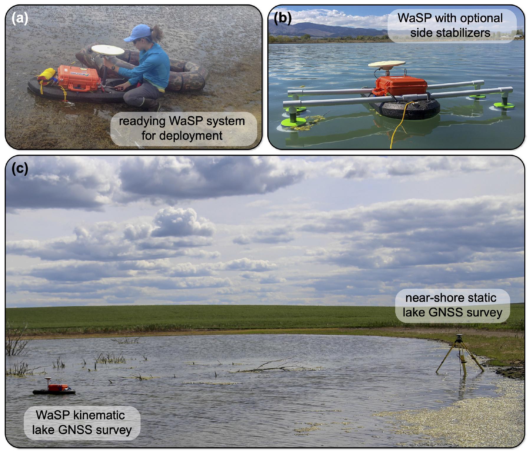
Figure 1. Example of (a) readying a Water Surface Profiler (WaSP) system for deployments, (b) a WaSP survey using optional side-stabilizers, and (c) a comparison between a WaSP kinematic survey and a near-shore static survey. The WaSP system integrates a GNSS receiver and a power system within a ruggedized, waterproof case mounted atop a custom-shaped, high-density foam float with an external antenna mount and fastening locations for towlines, anchors, and drogues. The subject identified in (a) kindly provided written informed consent for the publication of this image.
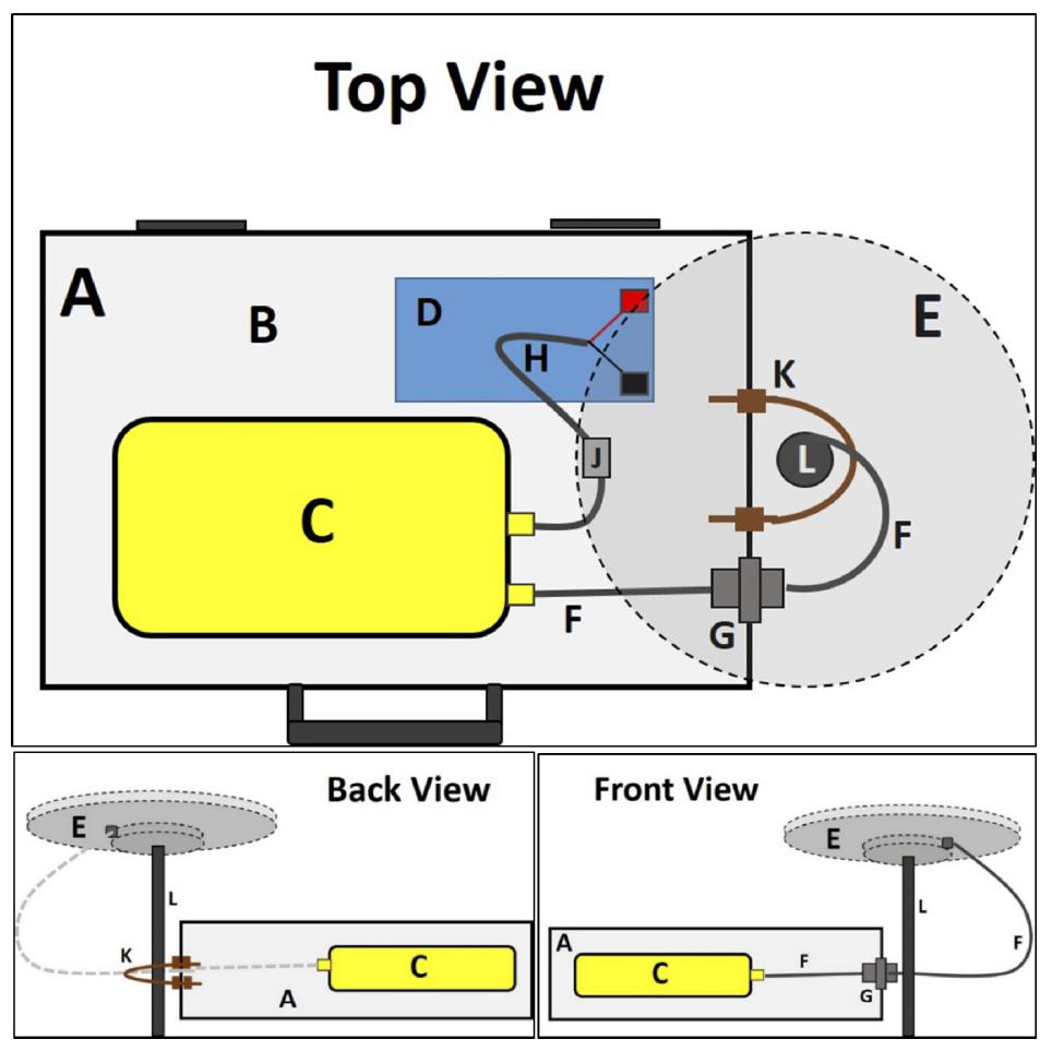
Figure 2. Schematic of WaSP receiver/antenna and power system from top view, back view, and front view. Water Surface Profiler components shown include (A) Pelican Case 1450; (B) Pelican Pick “n” Pluck foam; (C) GNSS receiver; (D) 12v 7Ah sealed lead-acid battery; (E) GNSS antenna; (F) RG-58 coaxial antenna cable with male TNC connectors; (G) TNC bulkhead, female-female, with watertight gasket; (H) power cable; (J) 3A automotive fuse; and (K,L) antenna mount with 5/8–11 threads.
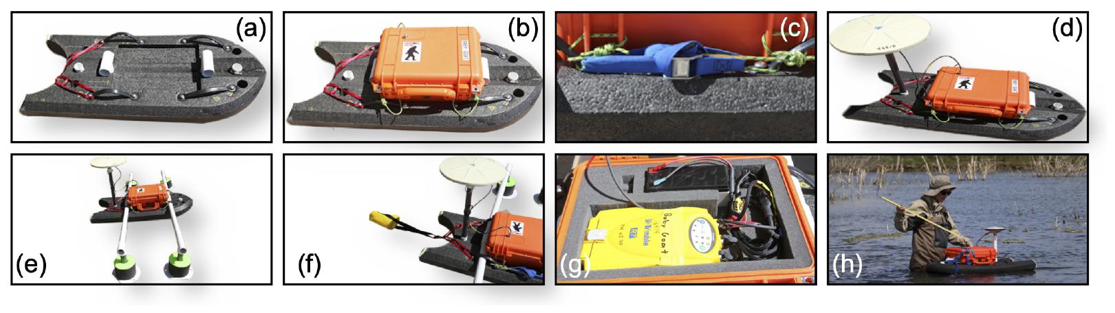
Figure 3. Water Surface Profiler is deployed using a (a) custom-shaped and designed high-density foam float. The case (b) containing the (g) power system and GNSS receiver is (c) secured to the float using Prusik knots, cam straps, and side handles. The (d) GNSS antenna is placed atop a mast, affixed to the float, and connected to the TNC bulkhead on the case. There are (e) optional side stabilizers that can be used in still water conditions. A (f) drogue and/or anchor system can be used for river or lake/pond surveys. To begin a survey, the (g) receiver needs to be powered on and connected to the antenna via the TNC bulkhead on the inside of the case. The (h) offset between the water surface and the antenna must also be manually measured, and a location with a clear sky view should be selected. The subject identified in (h) kindly provided written informed consent for the publication of this image.
GNSS Receiver and Antenna
WaSP can integrate most GPS/GNSS receiver and antenna combinations, as long as the form factor of the receiver (length to width ratio) is appropriate for the waterproof case enclosure (see Enclosure). The 2017 WaSP field surveys presented here were deployed using Trimble 5700 and R7 receivers and Zephyr Geodetic antennas. WaSP has also been deployed using Septentrio PolaRX-5 receivers and Septentrio PolaNt-x MF antennas.
Antennas are mounted at the highest point on WaSP to ensure maximum sky view and limit multipath interference from other components. The antenna mast is secured to the float using slit PVC pipe tensioned with a hose clamp. When possible, we recommend using small profile antennas to limit system weight and awkwardness during deployment and to maintain a low wind profile. Additional receiver and antenna integration considerations are detailed in Supplementary Text 1.1.1.
Power System
WaSP power requirements depend on receiver model/configuration and ambient temperature. For single day use with either a Trimble 5700/R7 or Septentrio PolaRX-5 receiver in Arctic and sub-Arctic environments, we recommend a 7-Ah AGM battery. WaSP power cables were adapted for use with the battery selected by both shortening the cable and terminating bare ends with tab connectors to fit the battery terminals. Additionally, a 3A fuse was added in line to the positive lead as protection for the receiver from short circuits or power surges. Additional power considerations are detailed in Supplementary Text 1.1.2.
Enclosure
The receiver, battery, and internal cabling are housed in a Pelican 1450 case. Components inside the case were separated and protected using Pick “n” Pluck foam provided by Pelican. The case is mounted on the float (Figure 3a) using Prusik knots tied through holes drilled into plastic ribbing on the external front and back of the Pelican Case (Figure 3b). The case is then secured using cam strap fasteners that run through the Prusik and tie point handles on the float (Figure 3c). This fastening system enables access to the case during deployment (Figure 3g). Because of the sensitivity of the GNSS equipment contained within the case, good waterproofing is required, both on the seal around the lid and the holes drilled for the antenna bulkhead. This can be accomplished with either rubber gaskets or marine-grade silicone sealant. In initial waterproofing tests, the modified case was filled with batteries and completely submerged for 5 minutes. No water intrusion was detected. It is recommended that seals be checked before deployment and replaced as needed.
Given that the WaSP system is deployed on water, it is important to ensure that weight is evenly distributed so that the system stays horizontal, and the antenna remains level. The battery is the heaviest component of the system, and thus, the final layout of the receiver and battery within the enclosure should be chosen to be as close to level as possible along the long axis (Figure 3g).
WaSP Float
The WaSP float is constructed using a durable, expanded polyethylene foam that repels water. The float is hand cut, glued, and shaped using routers with custom constructed molds. The shape includes a nose rocker, which reduces the likelihood of the system submerging, and is particularly important for towed deployments. The deck contains slanted grooves, which help drain water from the surface. The nose is protected by a polyurethane bumper and the bottom is flat with a slick-skin hot air welded finish for ruggedness and durability.
A recessed compartment for the Pelican Case 1450 is routed into the deck, and four handles are secured through the float surrounding the corners of the Pelican Case recess (Figure 3a). These handles provide tie-points for securing the case to the float (Figure 3c) and enable easy transport. A ∼4 cm outer-diameter slit PCV pipe is routed through the deck at the front and rear of the Pelican Case (Figures 3a,b). These provide attachment points for the antenna mast (Figures 3d,e), anchors if deployed in lakes/ponds, or tether points if deployed in rivers (Figure 3f). There are also optional side-stabilizer arms with polyethylene water wings that mount into two PVC T-brackets both secured into the foam (Figure 3e). We find that these stabilizers can induce an additional drag, which results in increased system drift, especially in windy lake/pond surveys. Furthermore, given the sufficiently high data precision attained without side stabilizers (see section “WaSP and Near-Shore Static Surveys in Prairie Pothole Ponds, Saskatchewan”), we do not recommend deploying side-stabilizers. Additional details about the float are given in Supplementary Text 1.1.3.
WaSP Deployment
An important consideration for WaSP accuracy is site selection. If deploying in a pond/lake, it is important that WaSP is located near the middle of the water body and away from metal docks, boats, or other obstructions (cliffs, trees, etc.). If there is a depth logger in the lake, WaSP should be placed near the instrument with the maximal clear sky view for optimal satellite trilateration.
Prior to deploying a WaSP unit in the field, it is important to enable at least one logging session on the receiver and make sure that batteries are fully charged. After this, field setup can be quickly completed at each site. First, insert the Pelican Case into the recess in the center of the float (Figures 3a,b) and secure it to the float by routing each Prusik through its neighboring handle and tethering Prusiks on the same side of the float with a cam strap (Figure 3c). Next, carefully insert the antenna mount into the PVC through-hole on the back of the float and mount the antenna to the mast (Figure 3d). Attach a coaxial cable to the antenna and TNC bulkhead on the Pelican Case (Figure 3d) and then attach a drogue and/or anchor system to the float using the webbing at the back of the board and PVC-lined hole at the front of the board (Figure 3f).
The optimal anchor/drogue configuration is site dependent. For example, in large lakes with rough water, a Danforth-style fluke anchor may be most appropriate. In small, calm ponds, a lightweight, folding Grapnel-style anchor may suffice. When towing a WaSP with a boat, a drogue is recommended for added stability.
To record data, open the Pelican Case, connect the antenna cable to both the interior TNC bulkhead and the receiver, and connect the power cable first to the battery and then the receiver (Figure 3g). It is important to cover exposed battery terminals to prevent cable movement and/or accidental shorting. GNSS receivers have model-dependent protocols to initiate logging. However, ensure that the receiver is powered on, observing satellites and recording data. Then, carefully tuck cables into the box and close/secure the lid.
Lastly, place the WaSP system in the water, fix the antenna mast height, and tighten it in place. Next, use a folding ruler or survey rod to measure the vertical offset between the antenna and the water surface (Figure 3h). We recommend measuring the vertical offset from at least three locations on the antenna and remeasuring offsets upon WaSP recovery to make sure that the offset remained constant during the survey. Note that antenna offsets can be measured relative to the antenna measurement point or the antenna reference point, given that appropriate, antenna-specific offsets are applied in data processing. Finally, we recommend taking photographs of the field site and making note of environmental conditions such as calm versus rough water as this may assist in data processing.
WaSP Data Processing
The first step in calculating WSE for WaSP surveys using Trimble or Septentrio receivers is to convert native GNSS data to the Receiver Independent Exchange Format (RINEX) file type, a commonly used ASCII file format that can be opened with most text readers. GNSS surveys recorded by Trimble 5700/R7 receivers are stored as .tXX Trimble data files, whereas surveys recorded by Septentrio receivers are stored as .SBF Septentrio Binary Format data files. For Trimble files, we use Trimble’s Convert To RINEX–TBC utility version 3.0.5.0, which is freely available via the Trimble website. For Septentrio receivers, we use SBF Converter, which is part of the Septentrio RxTools software package, which is freely available via the septentrio website. When a GNSS survey is recorded as multiple files, we use TEQC software, freely available from UNAVCO, to splice files together (see Supplementary Text 1.1.3 for pseudo TEQC syntax).
Next, the spliced RINEX file is submitted for postprocessing using PPP software. For the WaSP demonstration in the North Saskatchewan river and three prairie pothole ponds presented here (see section “WaSP and Near-Shore Static Surveys in Prairie Pothole Ponds, Saskatchewan, and North Saskatchewan River”), the Canadian Spatial Reference System–PPP web application is used, which is freely available via the Natural Resources Canada website.3 Specifically, the ellipsoidal height data contained within the .pos output file, relative to the International Terrestrial Reference Frames (ITRF, as defined by the International GNSS Service at the epoch for the specific orbit ephemerides), are used. For the 63 lake surveys spanning ∼17° latitude and ∼476 m vertical elevation collected during 2017 NASA ABoVE airborne sorties (section “Future WaSP Improvements”), PPP solutions are calculated using GINS software [developed by the Centre National d’Etudes Spatiales (CNES) and the Groupe de Recherche en Géodésie Spatiale (GRGS); Marty et al., 2011] and the International GPS Service precise GPS orbit and clock products. Resultant WSEs are given relative to the WGS84 ellipsoid. Note that the ITRF and WGS84 reference frames are quite similar, yet there are centimetric level absolute differences that spatially and temporally vary. For AirSWOT versus WaSP WSE comparisons (see section “North Saskatchewan River”), we do not apply a correction for the ellipsoid differences because the expected decimeter scale AirSWOT WSE uncertainty (Altenau et al., 2017; Pitcher et al., 2019; Tuozzolo et al., 2019) is much larger than the centimetric scale uncertainty associated with the different ellipsoids.
For the North Saskatchewan river data (see section “North Saskatchewan River”), we also convert from ellipsoidal heights (h) to orthometric heights (H), as follows:
where n is the height of the EGM96 geoid. Conversion from ellipsoidal to orthometric heights is particularly important for calculating WSS from longitudinal river surveys and in large, low-gradient lakes.
For lakes and ponds, the latitude, longitude (Figure 4A), and height (Figure 4B) data series from PPP results are analyzed, the field measured offset between the antenna and the water surface is applied (see WaSP Deployment), and the data series is manually subset using time windowing in TEQC (see Supplementary Text 1.1.4 3 for pseudo syntax) to a period in which WaSP is in the water and relatively stable (orange circles, Figures 4A,B). After time windowing, prairie pothole pond survey times ranged from 1 to 4 h (see section “WaSP and Near-Shore Static Surveys in Prairie Pothole Ponds, Saskatchewan”), whereas NASA ABoVE survey times varied from 0.9 to 10.4 h (see section “Future WaSP Improvements”).
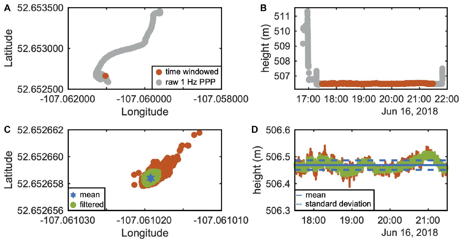
Figure 4. Water Surface Profiler (WaSP) data processing for lake/pond surveys requires first analyzing the original latitude, longitude (A) and height (B) data series (gray circles) and clipping the survey to times when the system is in the water, and there is minimal vertical and horizontal drift (orange circle). An outlier filter is then applied to the latitude, longitude (C), and height (D) data (green circles), and the average values are preserved [blue star in (C) and blue solid line in (D)].
Next, we use a Hampel filter with a 600-point window (10 min with 1 Hz logging interval) and 1.5 sigma threshold to remove outliers from the data series. A Hampel filter defines the median of a moving window and replaces outliers with the median value. Such filtering can be achieved using proprietary software such as MATLAB, or open-source software such as Python. The mean latitude, longitude (Figure 4C), and height (Figure 4D) of the windowed and filtered GNSS time series data are calculated as the final vertical and horizontal coordinates. Measurement uncertainty for a lake/pond (εl) survey is then calculated as
where σh is the standard deviation of 1 Hz heights from WaSP PPP solutions, σt is the standard deviation of antenna offset measurements, and the additional 0.01 m is intended to account for antenna offset measurement error. Note that the mean horizontal coordinates are representative, not an exact survey location because the WaSP systems move even during anchored lake/pond surveys.
For rivers, initial PPP results are converted to a .shp file and overlaid on nearly coincident satellite or airborne imagery in GIS software. The .shp file is visually inspected and locations in the data series when WaSP is not in transect are manually removed (red circles, Figure 5). This can be achieved using proprietary software packages such as ESRI’s ArcMap, or open-source software such as QGIS. After filtering, the North Saskatchewan River WaSP surveys presented here ranged from 9.29 to 9.40 h in duration, resulting in an average travel speed of 4.80 km/h.
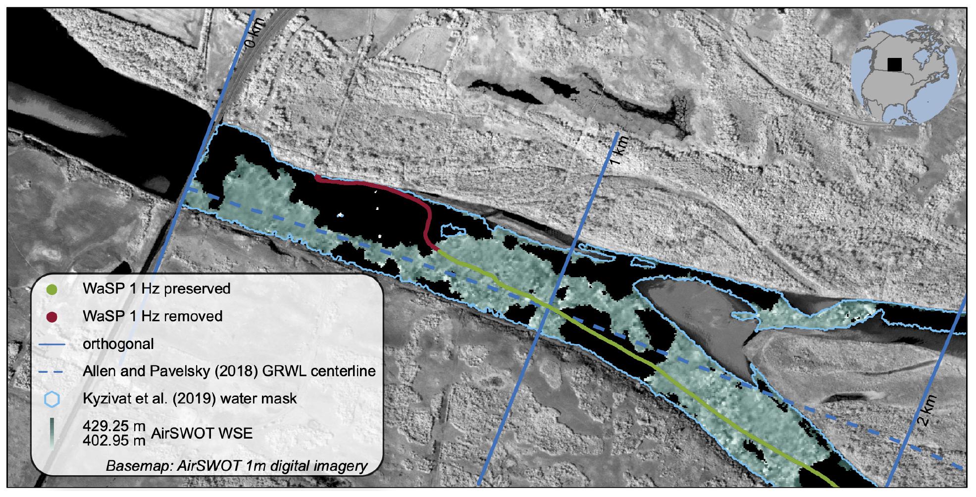
Figure 5. Water Surface Profiler data processing for river surveys requires manually inspecting the data series and removing points when the system is not in the water or in transect (red circles). Next, latitude, longitude, and height positions are assigned a downstream distance by snapping to their nearest-neighbor channel orthogonal (blue line). Here, we use the GRWL data to establish a channel centerline (Allen and Pavelsky, 2018). For cartographic clarity, orthogonals are shown at 1 km downstream intervals. Similarly, for comparisons between WaSP surveys (green circles) and AirSWOT mappings (green-to-white raster gradient), the AirSWOT data is first clipped to an open-water mask (teal polygon, from Kyzivat et al., 2019a,b) generated using 1 m resolution color-infrared digital orthomosaics (Kyzivat et al., 2018). AirSWOT pixels are also assigned a downstream distance by joining each pixel to its nearest-neighbor channel orthogonal. Note that locations within the water mask where there is no AirSWOT data are termed “dark water,” which occurs when there is insufficient radar reflectivity to interferometrically resolve a height. The base map is a 1 m resolution digital orthomosaic collected by AirSWOT on August 17, 2017, as part of the NASA Arctic Boreal Vulnerability Experiment.
Uncertainty in river WSE measurements (εr) is then calculated as follows:
where σh is the standard deviation of the estimated vertical positions from the NRCAN PPP output, and r is range in antenna offset measurements. Next, a centerline for the study reach is defined. For North Saskatchewan River results presented here, we use the Global River Widths from Landsat (GRWL) database (Allen and Pavelsky, 2018) and remove right angles from the centerline (Pitcher et al., 2019; Figure 5). Channel orthogonals are then established at right angles to the centerline at 25 cm downstream intervals (Ferreira, 2014; Figure 5). Lastly, 1 Hz GNSS solutions from filtered PPP .shp file outputs are assigned a downstream distance by joining each point with its nearest-neighbor channel orthogonal.
AirSWOT Radar Processing
AirSWOT is an airborne ka-band radar that produces swath-based maps of WSE (Altenau et al., 2017, 2019; Denbina et al., 2019; Pitcher et al., 2019; Tuozzolo et al., 2019). To map WSE, AirSWOT uses along-track interferometry, where two SAR images are taken along the flight track to create an interferogram. Using traditional InSAR processing techniques, phase differences shown in the interferogram indicate differences in elevation relative to the wavelength; such phase differences are used to produce an elevation model (e.g., Wu et al., 2011; Long and Ulaby, 2014). Here, we use AirSWOT data collected over the North Saskatchewan River on July 8, 2017, August 16, 2017, and August 17, 2017, to demonstrate how WaSP can be used to validate AirSWOT-like mappings of WSE. These data were collected as part of the 2017 NASA ABoVE airborne campaign (see section “Future WaSP Improvements”) and are freely available via the Oak Ridge National Laboratory Distributed Active Archive Center4 (Fayne et al., 2019). Each swath of AirSWOT radar data is delivered as a six-band geotiff with 3.6 × 3.6 m pixel size. Band 1 contains interferometrically derived heights, in meters, relative to the WGS84 ellipsoid. Bands 2 through 6 are the radar incidence angle (radians), magnitude [which can be converted to dB using 20∗log10(mag)], correlation (dimensionless), height sensitivity (meter/radian), and height uncertainty (as “error” in meters). See Fayne et al. (2020) for discussion of specific limitations of these data.
To aid interpretation of radar data, AirSWOT also integrates a color-infrared (CIR) digital camera. The images collected by the CIR system were processed into 1 m resolution orthomosaics (Kyzivat et al., 2018), which were then classified into binary open-water masks (Kyzivat et al., 2019b). The open-water classification uses on an object-based unsupervised classification routine, with manual quality control. A threshold was applied to a normalized difference water index (Mcfeeters, 1996) in order to identify open-water seed regions, and a custom region-growing procedure was developed to determine a final open-water boundary (Kyzivat et al., 2019a; Figure 5). Here, we use the open-water mask created from August 17, 2017, CIR data over the North Saskatchewan River to systematically remove non–open-water pixels from both July and August radar data. Note that of the 3 days surveyed by AirSWOT in 2017, North Saskatchewan River water levels were lowest on August 17, 2017 (Supplementary Figure 1). Therefore, we contend that the use of only the water mask from August 17, 2017, conservatively eliminates non–open-water pixels for all three sorties.
Raw AirSWOT radar data requires filtering to eliminate pixels with anomalous WSE values (Altenau et al., 2017; Pitcher et al., 2019). The filtering applied here includes first removing non–open-water pixels using the open-water mask (Kyzivat et al., 2019a,b). Second, the global MERIT DEM (Yamazaki et al., 2017) is used to remove pixels with WSE values greater or less than 5 m from MERIT (Fayne et al., 2020). MERIT DEM was selected because it has sufficient spatial coverage, is freely accessible to the research community, and employs careful merging/reprocessing of other commonly used DEMs (Yamazaki et al., 2017). Original MERIT DEM pixel heights are given relative to the EGM96 geoid. For comparison with AirSWOT, the EGM96 geoid is subtracted such that heights are relative to the WGS84 ellipsoid. Lastly, AirSWOT pixel values with random height error > 1 m are removed (Pitcher et al., 2019). After filtering, remaining AirSWOT WSE pixels are joined to their nearest-neighbor centerline orthogonal. When an orthogonal has > 1 nearest-neighbor AirSWOT pixels, these pixel WSEs are averaged. Lastly, all pixels are assigned a downstream distance (in streamwise kilometer from the Petrofka Bridge), enabling direct comparison with WaSP WSE surveys.
North Saskatchewan River Motorboat GNSS Surveys
Accompanying July 7, 2017, and August 16, 2017, WaSP deployments on the North Saskatchewan River presented here (see section “North Saskatchewan River”), a GNSS receiver and antenna were affixed to a vertical mast on a motorboat and driven along the same reach. While this motorboat-mounted survey technique is a standard field measurement protocol for surveying WSE in rivers (e.g., Altenau et al., 2017), the motorboat data collection pattern was not optimized for longitudinal WSE and WSS surveys. That is, the primary objective of the motorboat team was to collect hydrographic surveys of water depth and velocity at downstream cross sections. Therefore, the motorboat made more turns and frequently approached the shore, likely leading to multipath errors and loss of geometry compared to WaSP surveys. Therefore, we present the motorboat data as validation of WaSP and refrain from commenting on the comparative accuracies of motorboat and WaSP WSE and WSS mappings.
North Saskatchewan River in situ Water Level Sensor Arrays
In addition to the WaSP and motorboat surveys, the Water Survey of Canada, a branch of Environment and Climate Change Canada (ECCC), installed and surveyed in an array of nine temporary pressure transducers (PTs) in the North Saskatchewan River study reach (Figure 7 and Supplementary Table 1). These PTs were programmed to measure WSE at 5 minute intervals, and all nine PTs were operational during July 2017 WaSP, motorboat, and AirSWOT surveys. This array is used as an independent validation of WaSP WSE (Figure 10A) and WSS (Figure 11A).
Unfortunately, data from only one of the nine PTs were recovered for the August 2017 surveys. The PT recovered was located 0.37 km from the start of the study reach, near Petrofka Bridge (Figure 7). The raw pressure data series from this PT was manually converted to water depth using a barometric pressure logger located near the end of the study reach (close to Wingard Ferry). Notable jumps in the data series suggest that the PT location shifted between installation and recovery. To rectify this, jumps in the data series were manually identified, and a constant offset calculated as the difference between neighboring high-quality measurements was applied to subsequent data readings. After manual adjustment, outlier readings from the 5 min data series were removed using a Hampel filter with a 288-point (or 1 day given a 5 min logging interval) window. Finally, the daily average was computed (Supplementary Figure 1 and Supplementary Table 2) and is used here to determine the total water level drawdown between July and August 2017 (Figure 10B).
Results
To test WaSP performance in lakes and rivers, we compare WaSP WSE and WSS mappings against traditional near-shore static and motorboat-mounted kinematic GNSS surveys, as well as field-deployed PTs. Such ancillary data are not required for WaSP validation of coincident airborne or spaceborne WSE or WSS mappings.
WaSP and Near-Shore Static Surveys in Prairie Pothole Ponds, Saskatchewan
WaSP units were deployed in three ponds near Saskatoon, Saskatchewan, Canada (Supplementary Figure 3). Deployments were conducted on July 4, 2017, August 17, 2017, and June 16, 2018, on Pond #1, and July 4, 2017, and August 17, 2017, on Pond #2 and Pond #3. In all three ponds, WSE dropped between July and August 2017. In Pond #1, WSE dropped from 506.55 to 506.35 m, a net drawdown of 20 cm (Figure 6A). Water surface elevation in Pond #2 and Pond #3 fell from 509.21 to 508.96 m and 498.87 to 498.71 m, and net drawdowns of 25 cm and 16 cm, respectively (Figures 6B,C). εl (Eq. 2) across the seven WaSP surveys in three ponds ranged from ∼3 to 5 cm.
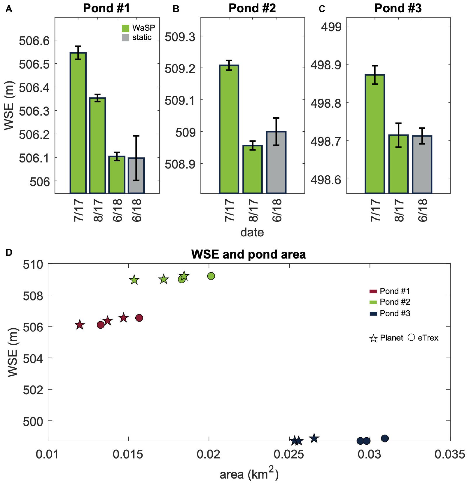
Figure 6. Three Prairie Pothole ponds near Saskatoon, Saskatchewan, Canada, were surveyed in July and August 2017 and June 2018 using WaSP and near-shore static tripod surveys. Outer shorelines were manually mapped in situ using handheld Garmin eTrex GPS’s and also hand digitized ignoring floating and/or inundated vegetation within the pond using Planet 3.125 m resolution satellite imagery (Planet Team, 2019) collected on July 4, 2017, August 18, 2017, and June 16, 2018. (A–C) Show resultant WaSP water surface elevation (WSE) surveys (green bars). Pond #1 (A) was surveyed in July and August 2017 and again in June 2018 using both a WaSP and a near-shore static survey (gray bar). Pond #2 (B) and Pond #3 (C) were surveyed using WaSPs in July and August 2017 and again in June 2018 using only a near-shore static survey. The (D) WSE changes in all three ponds covary with changes in inundation extent (eTrex) and shoreline area (Planet), which independently validates that WaSP data are both accurate and reproducible. The WSE values shown are ellipsoidal heights.
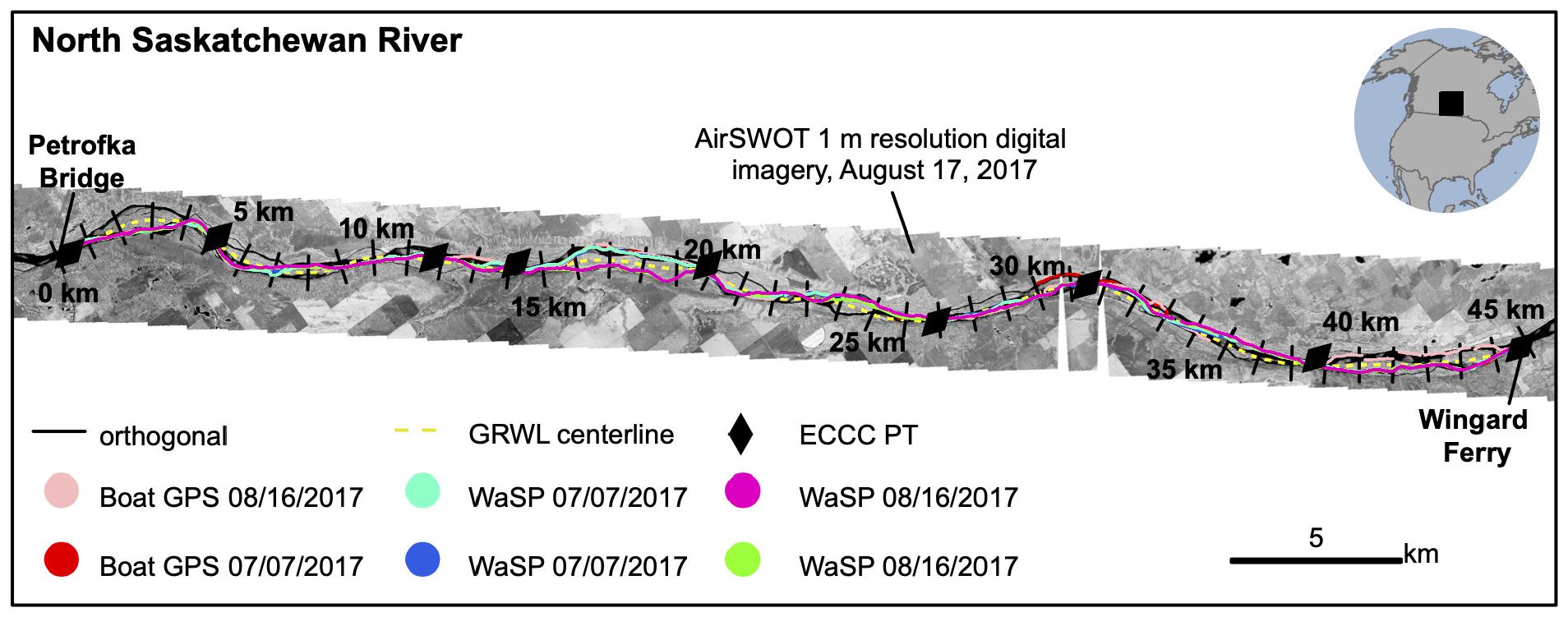
Figure 7. On July 7, 2017 (blue circles), and August 16, 2017 (green and magenta circles), WaSP systems were escorted down a ∼45 km reach of the North Saskatchewan River. A motorboat-mounted GNSS system similarly surveyed WSE in this reach (red circles). Environment and Climate Change Canada also installed nine pressure transducer (PT) water-level loggers (black diamonds), which are used here as an independent validation of WaSP. The river centerline (dashed yellow line) and channel orthogonals (solid black lines, created every ∼25 cm along the channel centerline, but shown at 5 km spacing) were used to establish the streamwise coordinates of WaSP, motorboat, and PT data. The base map is a 1 m resolution color-infrared orthomosaic collected by AirSWOT on August 17, 2017, as part of the NASA Arctic Boreal and Vulnerability Experiment (ABoVE).
These drawdowns also correlate with pond shoreline area, as manually mapped in situ using a handheld Garmin eTrex GPS and hand digitized in nearly coincident Planet 3.125 m resolution satellite imagery (Planet Team, 2019; Supplementary Figure 3). These ponds all have emergent vegetation. Therefore, eTrex shorelines represent inundation extent, whereas Planet digitizing represents shoreline areas. Given this difference, we expect Planet areas to be smaller than eTrex areas. WaSP measures WSE drawdowns between July and August 2017, which are accompanied by a reduction in both mapped (eTrex) and digitized (Planet) areas (Figure 6D and Supplementary Table 3). As expected, Planet areas are also smaller than eTrex areas. Near-shore static WSE surveys conducted the following spring find that water levels increased in all ponds between August 2017 and June 2018. These WSE increases were similarly accompanied by an increase in shoreline area in all three ponds (Figure 6D and Supplementary Table 3). These results suggest that WaSP can detect centimeter-scale changes in WSE.
On June 16, 2018, Pond #1 was surveyed using both WaSP and a near-shore static survey (Figure 1c), using identical Septentrio GNSS receivers, antenna combinations, and logging protocols. For the near-shore survey, a monument was pounded into the pond bottom; a tripod was leveled over the monument using a tribrach with an optical plummet; and offsets between the water surface, the top of the monument, and the antenna phase center were measured. The absolute WSE difference between the near-shore static and WaSP surveys was < 1 cm. This comparison between WaSP and standard near-shore static surveys suggests that WaSP lake surveys are reproducible.
North Saskatchewan River
On July 7, 2017, and August 16, 2017, WaSP units were tethered to canoes and towed down a ∼45 km reach of the North Saskatchewan River to measure longitudinal WSE and WSS between Petrofka Bridge and Wingard Ferry (Figure 7). To determine reproducibility of results, surveys on both days were conducted using two WaSP units, each outfitted with identical Trimble R7 receiver/Zephyr geodetic antenna combinations, loaded with the same 1 Hz logging sessions, and escorted downstream by two canoes and two field teams. The median absolute WSE difference between these WaSP systems was ∼3 cm on July 7, 2017, and ∼2 cm on August 16, 2017 (Table 1A). These differences are less than the median ∼6 to ∼7 cm εr (Eq. 3) associated with each survey (Table 1B), affirming that the WaSP platform yields reproducible results.
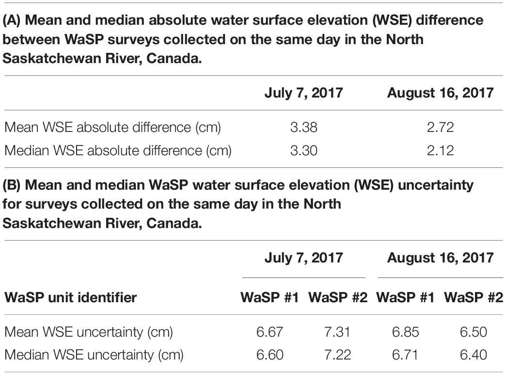
Table 1.
WaSP WSEs on July 7, 2017, are also similar to nine ECCC PTs surveyed in along our study reach (Figure 8). The absolute differences of the median WaSP WSE for 20 m reaches centered on each PT compared to an accompanying PT WSE range from 5 to 14 cm, with a median overall difference of 8 cm. The median WaSP WSE is also ±10 cm PT WSE for 8 out of the 9 PTs (Figure 10A), suggesting that longitudinal WaSP surveys measure WSE with accuracies exceeding SWOT requirements for 1 km2 open-water areas with 20 m or less downstream spatial averaging. See Supplementary Figure 2 for analogous comparisons between PT, motorboat, and AirSWOT.
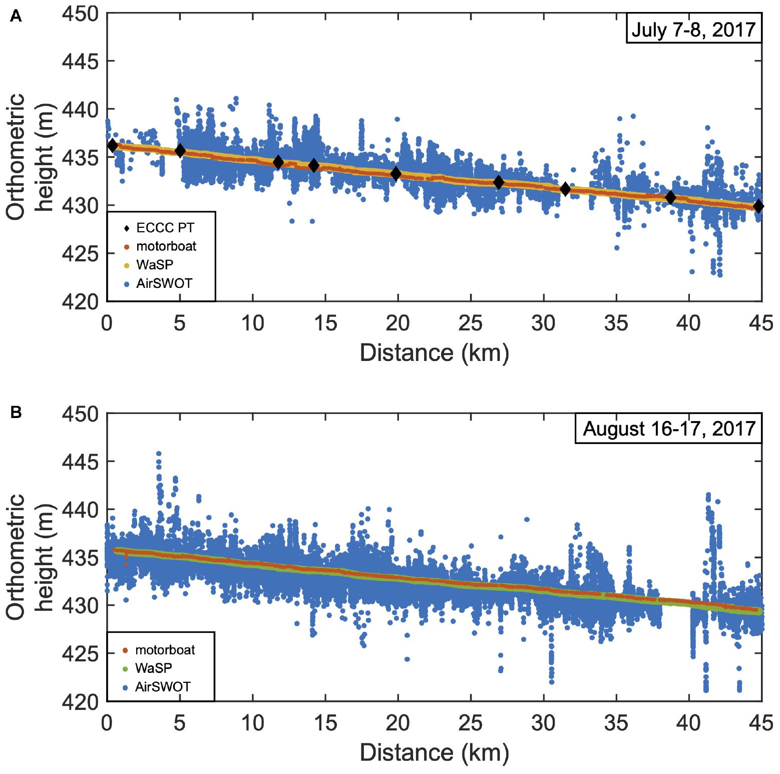
Figure 8. The Water Surface Profiler (WaSP) system is designed to be a standard and repeatable validation instrument for remotely sensed mappings of WSE. As a demonstration of this, (A,B) compare WaSP longitudinal profiles (yellow and green circles) along a ∼45 km reach of the North Saskatchewan River with nine pressure transducer (PT; black diamonds) water-level loggers, a motorboat-mounted GNSS survey, and AirSWOT mappings (blue circles) along the same reach on both (A) July 7–8, 2017, and (B) August 16–17, 2017. Note that the WSE values shown are orthometric heights. Outlier AirSWOT WSE values > 450 and < 420 m are not shown.
To further validate WaSP, longitudinal WSE profiles are compared with those mapped by the motorboat-mounted GNSS. Overall, the two longitudinal profiles (Figure 8) and resultant WSEs (Figure 9) are similar, but there are notable differences. First, given that the motorboat made several transects orthogonal to flow direction for hydrographic depth and velocity surveys, the WSE data had to be carefully inspected and manually filtered, resulting in data gaps (e.g., ∼21.7 km downstream; Figure 8A). Second, the angle of the antenna on the motorboat would tilt when weight on the boat was redistributed due to people or equipment moving. Third, the motorboat was unable to survey shallow reaches of the river. This was particularly problematic for the August 16, 2017, motorboat survey when the antenna height changed three times to accommodate shallow water conditions. This resulted in three unique vertical offset corrections that were applied to the final data series. Shallow water is not a problem for WaSP because the platform has low draft. Therefore, WaSP is equally capable of surveying WSE in shallow and deep water and is insensitive to weight redistribution due to people moving on the towboat. Such flexibility is notable in complex braided rivers and/or floodplains where shallow water conditions are common and WSE cannot be easily measured with point-based survey techniques.
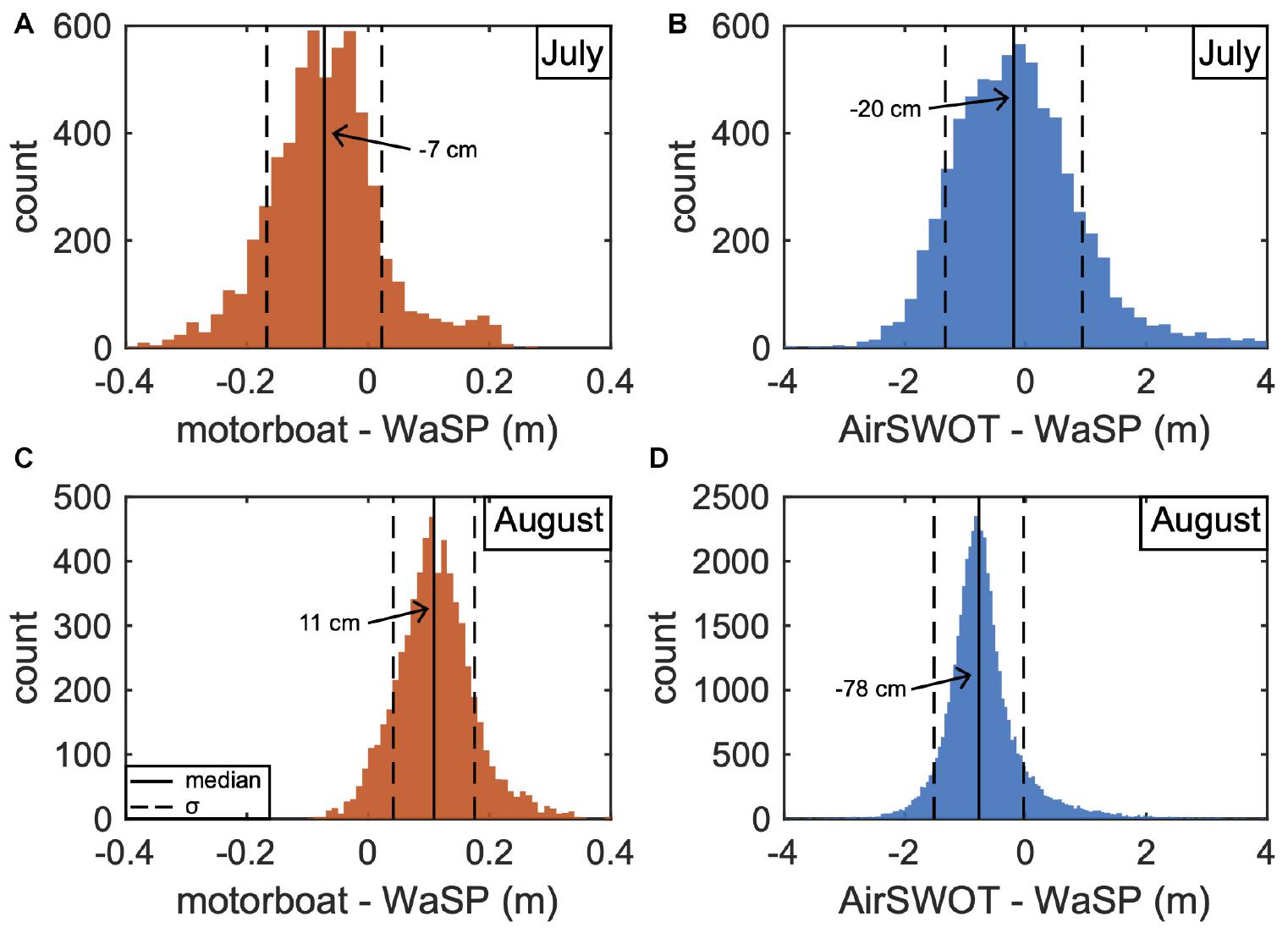
Figure 9. The WSE differences between motorboat (A,C), AirSWOT (B,D), and WaSP in July (A,B) and August, 2017 (C,D). Median differences (solid black line) and 1 standard deviation of the distribution of differences (σ; dashed black line) are plotted. Note that outlier differences falling outside of x-axis bounds are not shown.
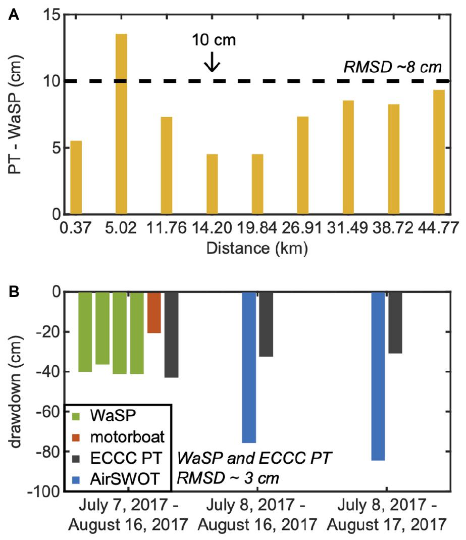
Figure 10. On July 7, 2017, the absolute WSE difference between (A) Environment and Climate Change Canada (ECCC) pressure transducer (PT) water-level loggers and WaSP averaged along 20 m reaches centered on each PT was < 10 cm (dashed black line) for eight of nine PTs. (B) shows the WSE drawdown between July and August measured by WaSP (green), motorboat (orange), AirSWOT (blue), and an ECCC PT (black) located near the Petrofka Bridge at the upstream end of our study reach. Drawdowns from WaSP closely match ECCC PT, suggesting that repeat WaSP surveys accurately quantify water level changes.
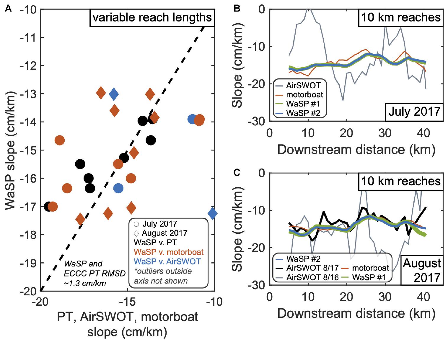
Figure 11. Comparison of (A) water surface slope (WSS) from WaSP (y-axis) and motorboat (orange; x-axis), AirSWOT (blue; x-axis) and Environment and Climate Change Canada (ECCC) pressure transducer (PT; black; x-axis), water-level loggers in July (circles) and August (diamonds) 2017. Reach lengths vary from ∼2.4 to 7.2 km and are defined by the downstream spacing between ECCC PTs. Note that PT data are not available in August 2017. Outliers WSS > −10 cm/km and < −20 cm/km are not shown. (B,C) Plot WSS for 10 km reaches established every 1 km downstream along the North Saskatchewan River. Water surface slope was surveyed by two WaSPs (green and blue lines), AirSWOT (gray and black lines), and a motorboat in (B) July 2017 and (C) August 2017.
The primary motivation for WaSP development is to validate AirSWOT and forthcoming SWOT mappings of WSE and WSS. To test WaSP’s suitability for this task, we compared WaSP WSE surveys on the North Saskatchewan River collected on July 7, 2017, and August 16, 2017, with nearly coincident AirSWOT mappings of the same reach collected on July 8, 2017, August 16, 2017, and August 17, 2017. Unfortunately, ∼84, 87, and 45% of the study reach water surface area on these dates was not mapped by AirSWOT because of poor radar reflectivity as the radar signal scatters away from the sensor at higher incidence angles (commonly referred to a “dark water”). Because of the lack of available data, the downstream spatial averaging of open-water pixels required to test SWOT accuracy requirements (Rodriguez, 2016) was not possible in this analysis. Despite this limitation, a pixel-based AirSWOT WSE and WSS to WaSP comparison was conducted.
Figure 8A shows downstream WaSP WSE (yellow circles) compared with PT WSE (black diamonds), motorboat WSE (orange circles), and AirSWOT WSE (blue circles) on July 7 to 8, 2017, and Figure 8B compares WaSP WSE (green circles) with motorboat WSE (orange circles) and AirSWOT pixels (blue circles) on August 16 to 17, 2017. These subplots show similar longitudinal profiles for both AirSWOT and WaSP. That is, the WSS calculated as the linear fit between WSE and downstream distance for the full study reach from WaSP is −16 cm/km on both July 7, 2017, and August 16, 2017, respectively. Slopes from AirSWOT are −14 and −15 cm/km on July 8, 2017, and August 16 to 17, 2017, respectively. While the longitudinal profiles are similar, the absolute WSE differences between WaSP and AirSWOT are inconsistent (Figures 9B,D). The median difference between AirSWOT and WaSP was −20 and −78 cm on July 7 to 8, 2017, and August 16 to 17, 2017, respectively. AirSWOT is biased (lower) during both surveys, with an inconsistent absolute bias as August mappings are nearly three times lower than July. Again, it is important to emphasize that, in order to meet accuracy requirements, AirSWOT and SWOT data require downstream spatial averaging. Because of lack of data density, such spatial averaging is not performed, and thus the accuracy of 2017 AirSWOT mappings in terms of SWOT mission requirements is not assessed. Despite this limitation, these results confirm that WaSP is a standard, repeatable, and flexible solution for validating remotely sensed estimates of WSE from platforms such as AirSWOT.
Figure 11A compares WSS measured by WaSP with PT, motorboat, and AirSWOT for the reach lengths ranging from 2.44 to 7.23 km established between downstream PTs (Table 2A). For PTs, slope is calculated as the dividend between the change in WSE and downstream distance (i.e., rise/run). For WaSP, motorboat, and AirSWOT, WSS is the slope of the linear fit between WSE and downstream distance. The root mean squared difference (RMSD; Table 2B) between WaSP and PT WSS on July 7, 2017, is 1.35 cm/km. The RMSD between WaSP and motorboat is also small, whereas the RMSD between WaSP and AirSWOT is > 15 cm/km (Table 2B). This confirms that when compared to traditional PT-based WSS, WaSP WSS accuracies over reaches as small as 2.44 km exceed the SWOT mission requirement of ± 1.7 cm/km for 10 km reaches at least 100 m wide (Rodriguez, 2016), suggesting that WaSP is a capable tool for AirSWOT and SWOT WSS validation.
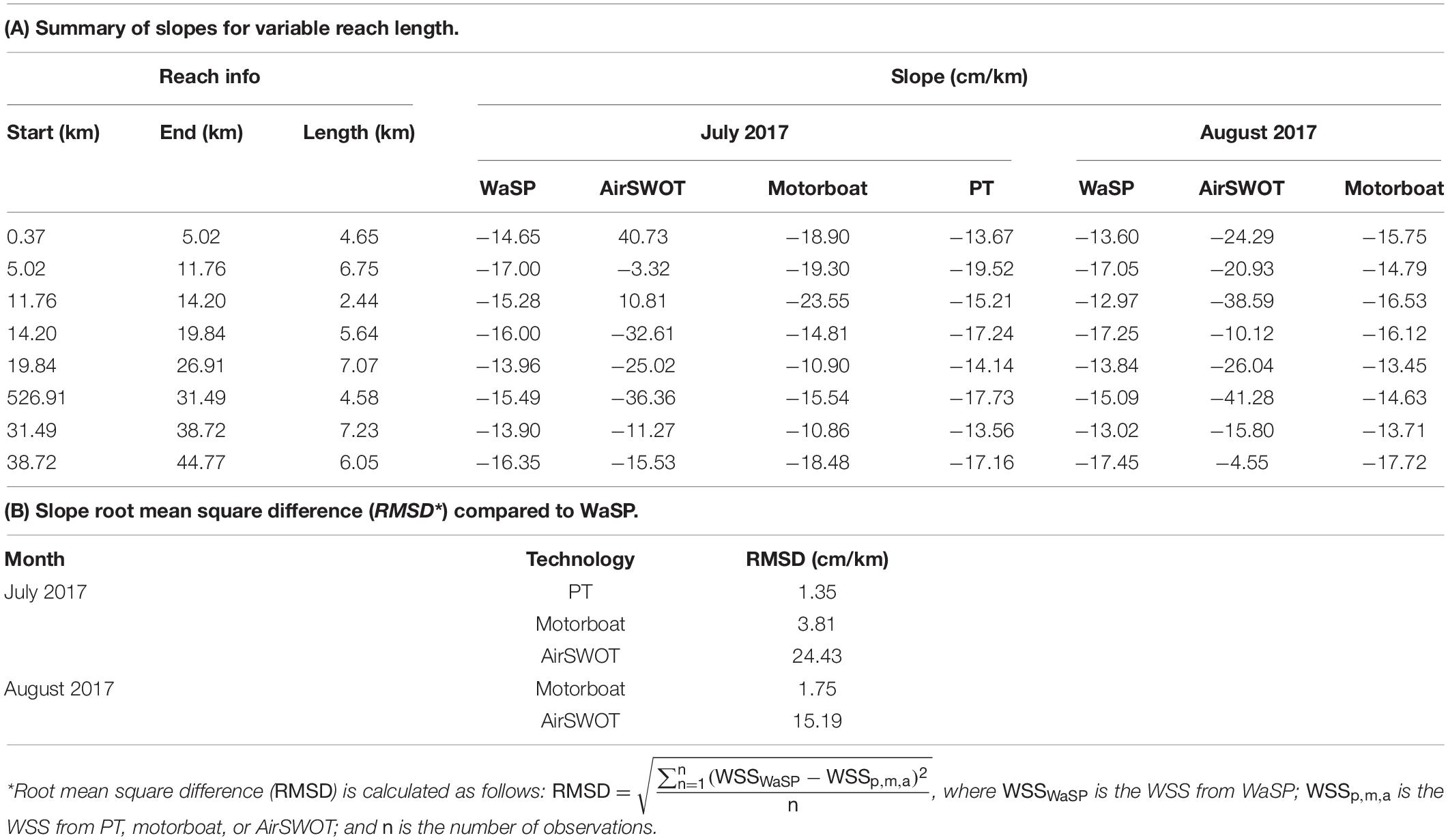
Table 2.
Figures 11B,C compare WSS for 10 km reaches measured by WaSP (blue and green lines), motorboat (orange lines), and AirSWOT (gray and black lines) in July (Figure 11B) and August 2017 (Figure 11C). WSS is calculated as the slope of the linear fit between WSE and distance for 10 km reaches established every 1 km downstream. In July and August, the absolute median difference in WSS from WaSP surveys was < 1 cm/km, emphasizing the repeatability of WaSP WSS. When comparing WaSP WSS with motorboat WSS, median absolute differences are also < 1 cm/km. Therefore, motorboat and WaSP WSS comparisons for 10 km reaches both meet SWOT requirements, again suggesting utility for future SWOT and AirSWOT validation. On August 17, 2017, the absolute median WSS difference between AirSWOT and WaSP was < 1.4 cm/km. On July 8, 2017, and August 16, 2017, the resultant absolute median WSS difference compared to WaSP was < 5.6 cm/km. Collectively, these results emphasize that, for 10 km reaches, WaSP correctly and consistently maps WSS with sufficient accuracy to validate AirSWOT and SWOT.
The power of multitemporal mappings of WSE is the ability to quantify water level changes and volumetric flux. To demonstrate this, Figure 10B compares median orthogonal WSE changes between July and August 2017 for WaSP (green bars), AirSWOT (blue bars), and motorboat GNSS data (orange bar) with in situ ECCC PT data (gray bars; see section “North Saskatchewan River In Situ Water Level Sensor Arrays”). The WaSP, AirSWOT, motorboat, and ECCC PT data all measure a net drawdown between the July and August 2017. However, the drawdown measured by these independent technologies differs. On average, WaSP measures a ∼39 cm drawdown compared to a ∼43 cm decrease measured by ECCC PT, a difference of ∼4 cm. In contrast, the difference between motorboat and ECCC PT data is ∼22 cm, whereas the difference between AirSWOT and ECCC is 42–54 cm for August 16 and August 17, 2017, surveys, respectively. These results suggest that repeat WaSP WSE surveys yield accurate water level changes that closely match standard field measurement methods.
Discussion
Overall WaSP Performance
These pond and river results yield important insights about WaSP overall performance. First, the subcentimeter difference between a WaSP and a near-shore-static survey in Pond #1 (Figure 6D), the minimal difference between nearly coincident WaSP river surveys (Table 1), and the close agreement with ECCC PT data (Figure 10A) suggest that WaSP yields reproducible data. Second, the comparisons between WaSP and AirSWOT suggest that WaSP is a standard and repeatable solution for validating remotely sensed estimates of WSE (Figure 9) and WSS (Figure 11). The strong agreement between shoreline areas and pond levels (Figures 6G–I), as well as the small absolute difference between WaSP drawdowns and ECCC PT data (Figure 10B), reveals that multitemporal WaSP surveys accurately reproduce water level drawdowns. Finally, the WaSP and PT WSE and WSS comparisons suggest that WaSP data accuracy is comparable to standard methods for surveying WSE and WSS. WaSP also has the added benefit of working equally well in shallow or deep water and is immune to the suite of shoreline conditions required for near-shore surveys. That said, it is important to note that this experiment does not explicitly investigate how hydraulic or climatic conditions influence WaSP data. We expect poor deployment conditions (e.g., high wind and/or rough water) to convolve with εr and εl.
WaSP Applications
To demonstrate the diverse capabilities of WaSP in scientific and practical applications, we describe several ways in which WaSP data is being collected and used. These applications are wide-ranging in their purposes, and our goal in describing them is to highlight the potential of WaSP based on the validation results presented in section “Results” and discussed in section “Overall WaSP Performance.”
WaSP Application 1: NASA SWOT Validation
SWOT is engineered to measure a number of key surface water hydrology variables, including WSE, WSS, inundation extent, river width, and river discharge in suitable reaches (Rodriguez, 2016). After launch, standard and reproducible field validation of these variables is needed. For at least three reasons, we propose WaSP as a standardized instrument for direct validation of WSE and WSS. First, when compared to PTs, WaSP WSE RMSD is ∼8 cm without any downstream spatial averaging (which, akin to SWOT and AirSWOT data processing, will reduce WSE uncertainty). This suggests that raw WaSP WSE data accuracy are appropriate for SWOT validation in rivers and lakes. Second, median WaSP WSS difference for 10 km reaches is < 1 cm/km when compared with motorboat GNSS surveys, and WSS RMSD is 1.3 cm/km when compared to PTs along reaches < 10 km, which is higher than that required by SWOT for 10 km reaches. Third, WaSP survey results are standard and repeatable, and the system is flexible and easy to deploy. This is ideal for a global satellite mission such as SWOT, because it enables validation across large spatial scales.
WaSP Application 2: Lake Surveys Supporting the NASA ABoVE
NASA ABoVE is a decadal project that aims to enhance understanding of ecological and social consequences of environmental change across Arctic and Boreal regions (Miller et al., 2019).5 In 2017, as a part of ABoVE, NASA deployed AirSWOT to map multitemporal WSE in rivers, lakes, and wetlands across Arctic and Boreal regions of Canada and Alaska. To validate AirSWOT WSE retrievals, dispersed field teams equipped with WaSP units were deployed to targeted locations under various AirSWOT overflights across the ABoVE study domain. In Canada, surveyed water bodies were either within Trail Valley Creek research watershed (Wilcox et al., 2019), near Yellowknife, or near Saskatoon. In Alaska, surveyed lakes were either within the Yukon Flats Basin, or the North Slope (Figure 12). The result is the largest known collection of airborne and field WSE measurements (Figure 12). Water Surface Profiler units were distributed to government field technicians and university partners, without prior field training. All surveys were successfully executed, which demonstrates the ease of use of WaSP. Furthermore, WaSP deployments were conducted on foot, by pack-raft, canoe, motorized boat, helicopter, and float plane. This highlights the flexibility of the system given different logistical conditions. In total, 63 WaSP WSE surveys were executed, spanning ∼17° latitude. Resultant GPS/GNSS data have been successfully processed using GINS PPP (Marty et al., 2011) software, and WSEs (Table 3) are being used to validate AirSWOT ABoVE mappings (Fayne et al., 2020).
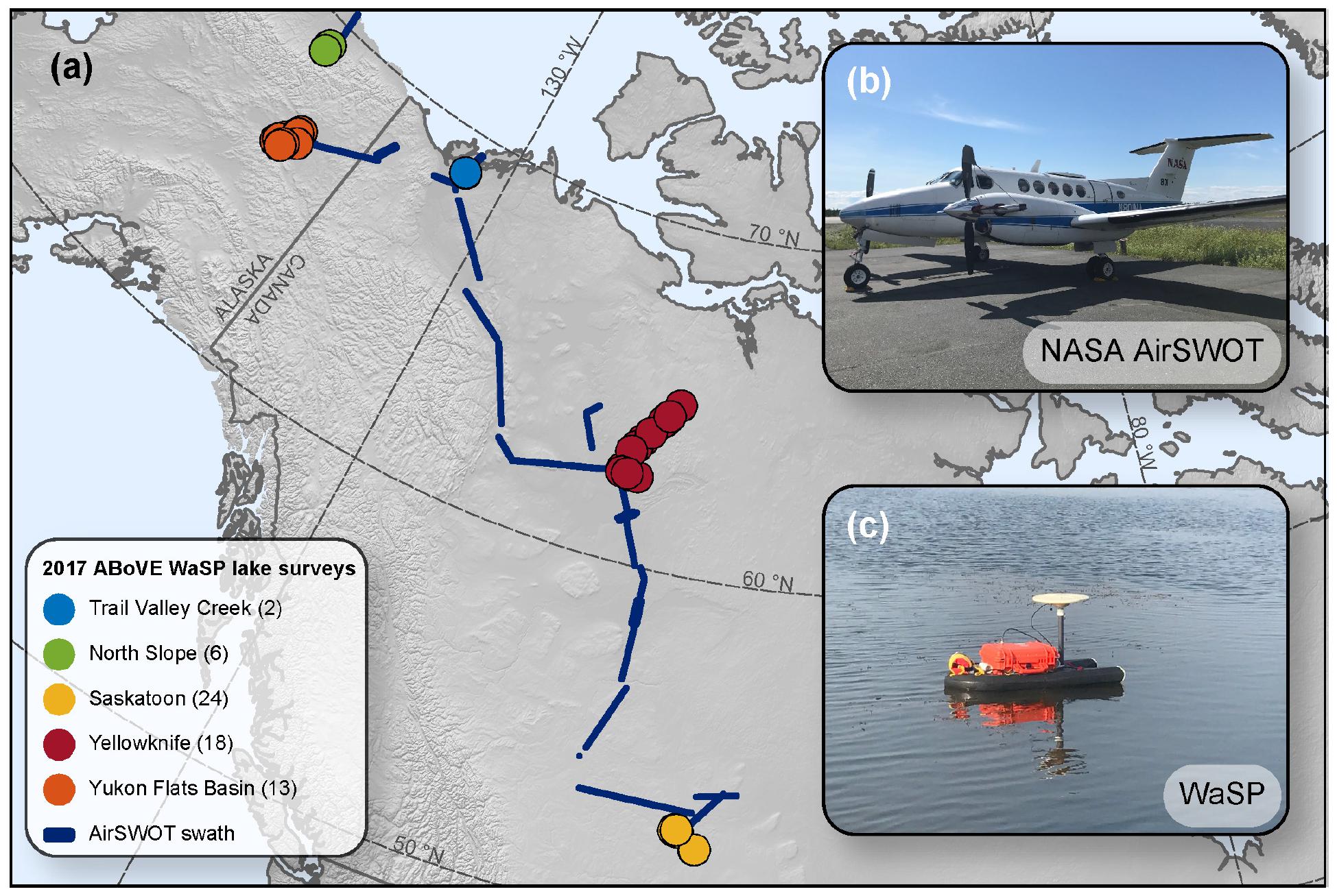
Figure 12. In 2017, WaSP was (a) deployed to remote regions of Canada and Alaska to validate (b) AirSWOT mappings of WSE that were commissioned by NASA Arctic Boreal and Vulnerability Experiment (ABoVE). In total, 63 WaSP (c) lake/pond surveys were executed, spanning ∼17° of latitude and ∼476 m of vertical elevation. Notably, WaSP surveys were successfully conducted by government scientists, academic partners, and field engineers alike and were deployed on foot, by kayak, truck, motorboat, floatplane, and helicopter. This highlights the flexibility of the WaSP system, which is particularly valuable for standard and repeatable validation of forthcoming global Surface Water and Ocean Topography (SWOT) satellite-based mappings of WSE and WSS.
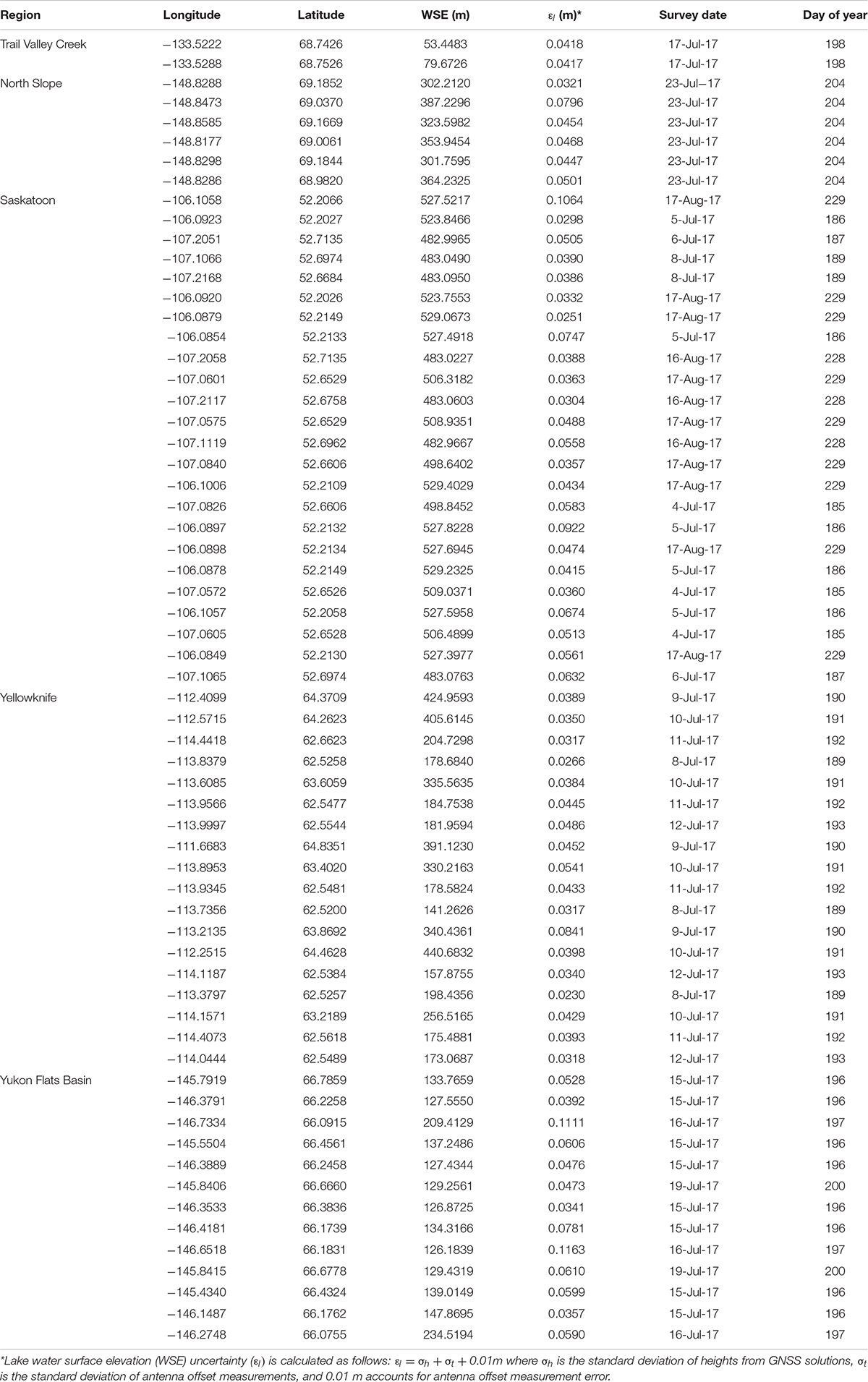
Table 3. Resultant water surface elevation (WSE) surveys from WaSP surveys in Canada and Alaska collected to validate 2017 NASA Arctic Boreal Vulnerability Experiment (ABoVE) AirSWOT sorties.
WaSP Application 3: Citizen Science Observations of Lake Storage
The Lake Observations by Citizen Scientists and Satellites (LOCSS) project aims to combine measurements of water level provided by citizen scientists with measurements of lake area from satellites to derive variations in lake water volume storage (Pavelsky et al., 2019).6 To date, LOCSS has deployed staff gauges into 62 lakes in the United States, France, and Bangladesh. Those in the United States have been leveled using WaSP WSE surveys. In each lake, WaSP systems were deployed adjacent to the staff gauge location for at least 1 h of continuous measurement. Resulting data were processed using the same methods described in section “WaSP Data Processing.” Citizen scientists provide gauge height measurements via SMS message or other methods, which can then be converted directly to WSEs using the WaSP surveys. To date, LOCSS has received > 5,500 height measurements from > 1,300 citizen scientists. WaSP surveys have been proven to be an effective means to determine lake WSE. Project staff received minimal training and successfully completed surveys of all lakes, suggesting that WaSP can be easily deployed with substantially less training than would be required by static shore-based surveys, which require leveling of an antenna on a tripod/tribrach assemblage. In the future, it would be possible to assess the consistency of citizen science and WaSP data by comparing multitemporal water level measurements from both methods.
WaSP Application 4: Validation of the LArge Wave Warning System
The LArge Wave Warning System (LAWWS) seeks to measure wave height in near real time and establish early warning alarms for coastal communities when large waves caused by significant landslides are detected. To achieve this, LAWWS relies on high-frequency GNSS interferometric reflectometry (GNSS-IR) measurements to detect real-time changes in WSE in relation to land mounted GNSS antennas. GNSS–IR has been previously used to detect storm surges (Peng et al., 2019), determine tidal stages (Larson et al., 2013a,b), and identify significant wave heights (Roggenbuck et al., 2019). However, because of limitations in the frequency of available GNSS data, it has not been possible to produce WSE in near real-time. Yet recent expansion in GNSS constellations makes it possible to utilize GNSS-IR to produce real-time observations of WSE, enabling their potential use in a robust early warning system (Peng et al., 2019; Reinking et al., 2019). To test this potential, LAWWS is deploying multiconstellation GNSS sites at The Nature Conservancy’s Jack and Laura Dangermond Preserve, in central California, to detect high-frequency WSE changes. WaSP systems will be temporarily anchored offshore and used to validate GNSS-IR measurements of sea surface and wave heights collected from a near-shore cliff-top. If successful, LAWWS will be deployed across at-risk coastal communities to provide a non-contact, early warning system for approaching large waves.
Future WaSP Improvements
The data presented here are from WaSP version 1. However, targeted deployments in support of NASA ABoVE and preplanning for NASA SWOT validation have illuminated system improvements that should be considered in future builds. First, a known source of uncertainty is the current necessity for manual antenna offset measurements. Future builds should consider fixed-height antennas and/or permanent metric markings. Second, the antenna mount can work loose in the foam over multiple deployments. This can be rectified by securing the antenna to the float and the Pelican Case. Third, more rocker, higher attachment points, and an asymmetrical boat-tethering system should be added to the float to minimize the risk of the nose pearling during longitudinal surveys. Fourth, stronger attachment points for anchors used during lake/pond surveys should be considered. Fifth, the side stabilizer should be removed to reduce weight/volume. Sixth, the Pelican Case insert could be upgraded to custom cut, closed-cell foam. Finally, the WaSP float has sufficient buoyancy that additional instruments could be integrated with the GPS/GNSS system. For example, a lightweight inertial measurement unit could be integrated to aid data processing. Similarly, integration of a high-frequency sonic roughness sensor and/or an optical sensor should be considered, specifically to improve AirSWOT/SWOT models of radar backscatter versus water surface roughness. Water quality sensors and bathymetric sonars could also be integrated with WaSP to broaden the scientific scope of the platform.
There are also field deployment and data processing techniques that could be improved. An initialization or a single-phase ambiguity resolution period consisting of a static survey with a duration of at least 15 min and up to an hour should be recorded prior to deploying WaSP in the water. Then the kinematic survey should begin continuously from the static collection. This static position can later be used in data processing to resolve atmospheric and positioning errors. The beginning of a kinematic survey can also be manually removed from both final positional averages and error compilations to minimize the impact of an initialization period.
Conclusion
Operational repeat mappings of WSE and WSS from the SWOT mission and its experimental validation instrument AirSWOT have the potential to transcend current limitations in monitoring global surface water resources. However, prior to forthcoming SWOT data being operationally adopted, direct field validation is needed. Such validation should be conducted in an accurate, efficient, standard, and repeatable manor. We thus propose the WaSP system as an operational tool for validating forthcoming SWOT data and as a standalone instrument for mapping large-scale hydraulics in lakes, wetlands, and rivers. WaSP has been successfully deployed in Arctic and Boreal regions of Alaska and Canada as part of the NASA ABoVE project, is operationally used as part of the LOCSS project, and will be used to aid development of a GNSS-IR–based LAWWS. WaSP is a rugged and flexible platform that can be deployed in a wide range of environments with minimal training. This ease of use and system flexibility are particularly useful for a global satellite mission like SWOT, because it allows validation at large spatial scales.
Data Availability Statement
All datasets generated for this study are included in the article/Supplementary Material.
Author Contributions
LP, AZ, RC, SC, and JP designed, tested, and built WaSP systems. LP, LS, and TP conceived of the manuscript. LP, AZ, TP, JH, and LS wrote the manuscript. LP and AZ made all the figures. LP, LS, SC, AZ, CG, JM, JF, MH, TL, ST, WD, EK, AP, PM, DY, TC, CO, EW, and TP collected the field data. LP and JF extracted the AirSWOT data. SC prepared the GPS/GNSS data for GINS PPP processing and summarized GINS outputs. MB-N, J-FC, and DM processed lake surveys using GINS. TC, NH, and CO prepared the Environment and Climate Change Canada (ECCC) Pressure Transducer (PT) data, and PT WSE surveys. MW, JH, and KE enabled discussion of LArge Wave Warming System (LAWWS). All authors reviewed manuscript and provided feedback.
Funding
This work was supported by the NASA Terrestrial Ecology Program Arctic-Boreal Vulnerability Experiment (ABoVE) Grant NNX17AC60A managed by Hank Margolis, NASA Surface Water and Ocean Topography (SWOT) mission Grant NNX16AH83G managed by Eric Lindstrom, NASA Surface Water and Ocean Topography (SWOT) mission Grant 80NSSC20K1144 managed by Nadya Vinogradova-Shiffer, and NASA Earth and Space Sciences Fellowship Program Grant NNX14AP57H managed by Lin Chambers.
Conflict of Interest
RC was employed by the company Carlson Designs.
The remaining authors declare that the research was conducted in the absence of any commercial or financial relationships that could be construed as a potential conflict of interest.
Acknowledgments
Equipment support and data services were provided by the GAGE Facility, operated by UNAVCO, Inc., with support from the National Science Foundation and the National Aeronautics and Space Administration under NSF Cooperative Agreement EAR-11261833. Processed AirSWOT radar data collected as part of 2017 NASA ABoVE campaign are available at: https://doi.org/10.3334/ORNLDAAC/1646 (Fayne et al., 2019). AirSWOT color-infrared orthomosaics collected as part of 2017 NASA ABoVE are available at: https://doi.org/10.3334/ORNLDAAC/1643 (Kyzivat et al., 2018). North Saskatchewan River water mask derived from AirSWOT color-infrared data collected as part of 2017 NASA ABoVE are available at: https://doi.org/10.3334/ORNLDAAC/1707 (Kyzivat et al., 2019b). We thank John Arvesen of Cirrus Digital Systems for assistance with color-infrared digital imagery; JPL AirSWOT processing team for radar data processing; Alex Shapiro of Alaska Land Exploration LLC for logistical and helicopter support out of Fairbanks, AK, USA; Jim Webster for floatplane support out of Fairbanks, AK, USA; Jerry Carrol in Fort Yukon, AK, USA for boat transport on the Yukon River; Heather Bartlett and Mark Bertram of the Yukon Flats National Wildlife Refuge for field support; Dave Olesen Hoarfrost River Huskies Ltd. for logistics and aircraft support out of Yellowknife, NWT, Canada; and Bruce Hanna (Government of the Northwest Territories Environment and Natural Resource Division) for assistance in collecting lake level records out of Yellowknife, NWT, Canada.
Supplementary Material
The Supplementary Material for this article can be found online at: https://www.frontiersin.org/articles/10.3389/feart.2020.00278/full#supplementary-material
Supplementary Figure 1 | Environment and Climate Change Canada (ECCC) pressure transducer (PT) water level record for one PT located 0.37 km from the start of our study reach. The original pressure data series (5 min logging interval) was manually converted to water depth using a barometric pressure logger located near Wingard Ferry at the end of the study reach (orange line). Notable jumps in the data series suggest that the PT location shifted between installation and recovery. To rectify this, jumps in the data series were manually identified and a constant offset, calculated as the difference between high-quality neighboring measurements was applied to subsequent data readings (dark blue line). Vertical gray bars denote WaSP and AirSWOT survey days.
Supplementary Figure 2 | The water surface elevation (WSE) difference between Environment and Climate Change Canada (ECCC) pressure transducer (PT) water level loggers and (A) WaSP, (B) motorboat, and (C) AirSWOT for 20 m reaches centered on each PT. Differences of ±10 cm are noted by dashed black line. Comparison is for surveys conducted on July 7–8, 2017 only. Analogous PT data is not available for August 2017 surveys.
Supplementary Figure 3 | Three Prairie Pothole ponds near Saskatoon, Saskatchewan, Canada (A–C) were surveyed in July and August 2017, and June 2018 using WaSP (green squares) and near-shore static tripod surveys (gray circles). Outer shorelines where manually mapped in situ using handheld Garmin eTrex GPS’s (pink vector lines) and also hand digitized ignoring floating and/or inundated vegetation within the pond using Planet 3.125 m resolution satellite imagery (Planet Team, 2019) collected on July 4, 2017, August 18, 2017, and June 16, 2018 (green and blue vector lines). The base map is a 1 m resolution digital orthomosaic collected by AirSWOT on August 17, 2017 as part of the NASA Arctic Boreal Vulnerability Experiment (ABoVE).
Footnotes
- ^ https://swot.jpl.nasa.gov/
- ^ https://swot.jpl.nasa.gov/mission/airswot/
- ^ https://webapp.geod.nrcan.gc.ca/geod/tools-outils/ppp.php
- ^ https://doi.org/10.3334/ORNLDAAC/1646
- ^ https://above.nasa.gov
- ^ http://locss.org
References
Allen, G. J., and Pavelsky, T. M. (2018). Global extent of rivers and streams. Science 361, 585–588. doi: 10.5268/IW-2.4.502
Alsdorf, D. E., and Lettenmaier, D. P. (2003). Tracking fresh water from space. Science. 301, 1491–1494. doi: 10.1126/science.1089802
Alsdorf, D. E., Lettenmaier, D. P., and Vörösmarty, C. J. (2003). The need for global, satellite-based observations of terrestrial surface waters. EOS Trans. Am. Geophys. Union Trans. 84, 269–276. doi: 10.1029/2003EO290001
Alsdorf, D. E., Rodríguez, E., and Lettenmaier, D. P. (2007). Measuring surface water from space. Rev. Geophys. 45:197. doi: 10.1029/2006RG000197
Altenau, E. H., Pavelsky, T. M., Moller, D., Lion, C., Pitcher, L., Allen, G. H., et al. (2017). AirSWOT measurements of river water surface elevation and slope: Tanana River, AK. Geophys. Res. Lett. 44, 181–189. doi: 10.1002/2016GL071577
Altenau, E. H., Pavelsky, T. M., Moller, D., Pitcher, L. H., Bates, P. D., Durand, M. T., et al. (2019). Temporal variations in river water surface elevation and slope captured by AirSWOT. Remote Sens. Environ. 224, 304–316. doi: 10.1016/j.rse.2019.02.002
Bates, P. D., Wilson, M. D., Horritt, M. S., Mason, D. C., Holden, N., and Currie, A. (2006). Reach scale floodplain inundation dynamics observed using airborne synthetic aperture radar imagery: data analysis and modelling. J. Hydrol. 328, 306–318. doi: 10.1016/j.jhydrol.2005.12.028
Biancamaria, S., Lettenmaier, D. P., and Pavelsky, T. M. (2016). The SWOT mission and its capabilities for land hydrology. Surv. Geophys. 37, 307–337. doi: 10.1007/s10712-015-9346-y
Crétaux, J. F., Abarca-del-Río, R., Bergé-Nguyen, M., Arsen, A., Drolon, V., Clos, G., et al. (2016). Lake volume monitoring from space. Surv. Geophys. 37, 269–305. doi: 10.1007/s10712-016-9362-6
Denbina, M., Simard, M., Rodriguez, E., Wu, X., Chen, A., and Pavelsky, T. (2019). Mapping water surface elevation and slope in the mississippi river delta using the AirSWOT Ka-band interferometric synthetic aperture radar. Remote Sens. 11, 1–26. doi: 10.3390/rs11232739
Dietrich, W. E., Smith, J. D., and Dunne, T. (1979). Flow and sediment transport in a sand bedded meander. J. Geol. 87, 305–315. doi: 10.1086/628419
Durand, M., Lee-Lueng, F., Lettenmaier, D. P., Alsdord, D. E., Rodriguez, E., and Esteban-Fernandez, D. (2010). The surface water and ocean topography mission: observing terrestrial surface water and oceanic submesoscale eddies. Proc. IEEE 98, 766–779. doi: 10.1109/JPROC.2010.2043031
Durand, M., Neal, J., Rodríguez, E., Andreadis, K. M., Smith, L. C., and Yoon, Y. (2014). Estimating reach-averaged discharge for the River severn from measurements of river water surface elevation and slope. J. Hydrol. 511, 92–104. doi: 10.1016/j.jhydrol.2013.12.050
Fayne, J. V., Smith, L. C., Pitcher, L. H., Kyzivat, E. D., Cooley, S. W., Cooper, M. G., et al. (2020). Airborne observations of Arctic-Boreal water surface elevations from AirSWOT Ka-band InSAR and LVIS LiDAR. Environ. Res. Lett. doi: 10.1088/1748-9326/abadcc
Fayne, J. V., Smith, L. C., Pitcher, L. H., and Pavelsky, T. M. (2019). ABoVE: AirSWOT Ka-Band Radar Over Surface Waters of Alaska and Canada, 2017. Oak Ridge, TN: ORNL DAAC.
Ferreira, M. (2014). Perpendicular Transects. Available at: https://gis4geomorphology.com/stream-transects-partial/ (accessed October, 2018).
Jowett, I. G. (1993). A method for objectively identifying pool, run, and riffle habitats from physical measurements. New Zeal. J. Mar. Freshw. Res. 27, 241–248. doi: 10.1080/00288330.1993.9516563
Kiel, B., Alsdorf, D., and LeFavour, G. (2006). Capability of SRTM C- and X-band DEM data to measure water elevations in ohio and the amazon. Photogramm. Eng. Remote Sens. 72, 313–320. doi: 10.14358/PERS.72.3.313
Kyzivat, E. D., Smith, L. C., Pitcher, L., Fayne, J. V., Cooley, S. W., Cooper, M. G., et al. (2019a). A high-resolution airborne color-infrared camera water mask for the NASA ABoVE campaign. Remote Sens. 11, 1–28. doi: 10.3390/rs11182163
Kyzivat, E. D., Smith, L. C., Pitcher, L. H., Fayne, J. V., Cooley, S. W., Cooper, M. G., et al. (2019b). ABoVE: AirSWOT Water Masks from Color-Infrared Imagery over Alaska and Canada, 2017. Oak Ridge, TN: ORNL DAAC.
Kyzivat, E. D., Smith, L. C., Pitcher, L. H., Pavelsky, T. M., Cooley, S. W., et al. (2018). ABoVE: AirSWOT Color-Infrared Imagery Over Alaska and Canada, 2017. Oak Ridge, TN: ORNL DAAC.
Larson, K. M., Löfgren, J. S., and Haas, R. (2013a). Coastal sea level measurements using a single geodetic GPS receiver. Adv. Space Res. 51, 1301–1310. doi: 10.1016/j.asr.2012.04.017
Larson, K. M., Ray, R. D., Nievinski, F. G., and Freymueller, J. T. (2013b). The accidental tide gauge: a GPS reflection case study from kachemak bay, Alaska. IEEE Geosci. Remote Sens. Lett. 10, 1200–1204. doi: 10.1109/LGRS.2012.2236075
Lee, H., Durand, M., Jung, H. C., Alsdorf, D., Shum, C. K., and Sheng, Y. (2010). Characterization of surface water storage changes in Arctic lakes using simulated SWOT measurements. Int. J. Remote Sens. 31, 3931–3953. doi: 10.1080/01431161.2010.483494
LeFavour, G., and Alsdorf, D. (2005). Water slope and discharge in the Amazon River estimated using the shuttle radar topography mission digital elevation model. Geophys. Res. Lett. 32:491. doi: 10.1029/2005GL023491
Long, D., and Ulaby, F. T. (2014). Microwave Radar And Radiometric Remote Sensing. Ann Arbor, MI: University of Michigan Press.
Marty, J. C., Loyer, S., Perosanz, F., Mercier, F., Bracher, G., Legresy, B., et al. (2011). “GINS: the CNES/GRGS GNSS scientific software,” in Proceedings of the 3rd International Colloquium Scientific and Fundamental Aspects of the Galileo Programme, ESA Proceedings WPP326, New York, NY.
Mcfeeters, S. K. (1996). The use of the normalized difference water index (NDWI) in the delineation of open water features. Int. J. Remote Sens. 17, 1425–1432. doi: 10.1080/01431169608948714
Miller, C. E., Griffith, P. C., Goetz, S. J., Hoy, E. E., Pinto, N., McCubbin, I. B., et al. (2019). An overview of ABoVE airborne campaign data acquisitions and science opportunities. Environ. Res. Lett. 14:080201. doi: 10.1088/1748-9326/ab0d44
Montgomery, D. R., Beamer, E. M., Pess, G. R., and Quinn, T. P. (1999). Channel type and salmonid spawning distribution and abundance. Can. J. Fish. Aquat. Sci. 56, 377–387. doi: 10.1139/f98-181
Ostrovsky, I., Yacobi, Y. Z., Walline, P., and Kalikhman, I. (1996). Seiche-induced mixing: its impact on lake productivity. Limnol. Oceanogr. 41, 323–332. doi: 10.4319/lo.1996.41.2.0323
Papa, F., Durand, F., Rossow, W. B., Rahman, A., and Bala, S. K. (2010). Satellite altimeter-derived monthly discharge of the Ganga-brahmaputra river and its seasonal to interannual variations from 1993 to 2008. J. Geophys. Res. Ocean. 115:C12013. doi: 10.1029/2009JC006075
Pavelsky, T. M., Ghafoor, S., Hossain, F., Parkins, G. M., Yelton, S. K., Little, S. B., et al. (2019). Monitoring the World’s lakes: progress from citizen science and remote sensing. Mag. Environ. Manag.
Peng, D., Hill, E. M., Li, L., Switzer, A. D., and Larson, K. M. (2019). Application of GNSS interferometric reflectometry for detecting storm surges. GPS Solut. 23, 1–11. doi: 10.1007/s10291-019-0838-y
Pitcher, L. H., Pavelsky, T. M., Smith, L. C., Moller, D. K., Altenau, E. H., Allen, G. H., et al. (2019). AirSWOT InSAR mapping of surface water elevations and hydraulic gradients across the Yukon flats basin. Alaska. Water Resour. Res. 552:274. doi: 10.1029/2018WR023274
Planet Team (2019). Planet Application Program Interface: In Space For Life On Earth. Available at: https://api.planet.com (accessed October, 2018).
Prowse, T. D., Beltaos, S., Gardner, J. T., Gibson, J. J., Granger, R. J., Leconte, R., et al. (2006). Climate change, flow regulation and land-use effects on the hydrology of the peace-athabasca-slave system; findings from the northern rivers ecosystem initiative. Environ. Monit. Assess. 113, 167–197. doi: 10.1007/s10661-005-9080-x
Reinking, J., Roggenbuck, O., and Even-Tzur, G. (2019). Estimating wave direction using terrestrial GNSS reflectometry. Remote Sens. 11:1027. doi: 10.3390/rs11091027
Rodriguez, E. (2016). Surface Water and Ocean Topography Mission (SWOT) Project: Science Requirements Document (Rev A). Available at: https://pdms.jpl.nasa.gov (accessed November, 2018).
Roggenbuck, O., Reinking, J., and Lambertus, T. (2019). Determination of significant wave heights using damping coefficients of attenuated GNSS SNR data from static and kinematic observations. Remote Sens. 11:409. doi: 10.3390/rs11040409
Smith, L. C. (1997). Satellite remote sensing of river inundation area, stage, and discharge: a review. Hydrol. Process. 11, 1427–1439. doi: 10.1002/(sici)1099-1085(199708)11:10<1427::aid-hyp473>3.0.co;2-s
Tuozzolo, S., Lind, G., Overstreet, B., Mangano, J., Fonstad, M., Hagemann, M., et al. (2019). Estimating river discharge with swath altimetry: a proof of concept using AirSWOT observations. Geophys. Res. Lett. 46, 1459–1466. doi: 10.1029/2018GL080771
Wilcox, E. J., Keim, D., de Jong, T., Walker, B., Sonnentag, O., Sniderhan, A. E., et al. (2019). Tundra shrub expansion may amplify permafrost thaw by advancing snowmelt timing. Arct. Sci. 5, 202–217. doi: 10.1139/as-2018-0028
Wu, X., Hensley, S., Rodriguez, E., Moller, D., Muellerschoen, R., and Michel, T. (2011). “Near nadir Ka-band SAR interferometry: SWOT airborne experiment,” in Proceedings of the IEEE International Geoscience and Remote Sensing Symposium, Vancouver, BC.
Keywords: ABoVE, SWOT, GNSS, water surface elevation, water surface slope
Citation: Pitcher LH, Smith LC, Cooley SW, Zaino A, Carlson R, Pettit J, Gleason CJ, Minear JT, Fayne JV, Willis MJ, Hansen JS, Easterday KJ, Harlan ME, Langhorst T, Topp SN, Dolan W, Kyzivat ED, Pietroniro A, Marsh P, Yang D, Carter T, Onclin C, Hosseini N, Wilcox E, Moreira D, Berge-Nguyen M, Cretaux J-F and Pavelsky TM (2020) Advancing Field-Based GNSS Surveying for Validation of Remotely Sensed Water Surface Elevation Products. Front. Earth Sci. 8:278. doi: 10.3389/feart.2020.00278
Received: 27 November 2019; Accepted: 17 June 2020;
Published: 23 November 2020.
Edited by:
David Glenn Chandler, Syracuse University, United StatesReviewed by:
Hongkai Gao, East China Normal University, ChinaThibault Catry, Institut de Recherche pour le Développement (IRD), France
Copyright © 2020 Pitcher, Smith, Cooley, Zaino, Carlson, Pettit, Gleason, Minear, Fayne, Willis, Hansen, Easterday, Harlan, Langhorst, Topp, Dolan, Kyzivat, Pietroniro, Marsh, Yang, Carter, Onclin, Hosseini, Wilcox, Moreira, Berge-Nguyen, Cretaux and Pavelsky. This is an open-access article distributed under the terms of the Creative Commons Attribution License (CC BY). The use, distribution or reproduction in other forums is permitted, provided the original author(s) and the copyright owner(s) are credited and that the original publication in this journal is cited, in accordance with accepted academic practice. No use, distribution or reproduction is permitted which does not comply with these terms.
*Correspondence: Lincoln H. Pitcher, bGluY29sbi5waXRjaGVyQGNvbG9yYWRvLmVkdQ==; bGluY29sbnBpdGNoZXJAdWNsYS5lZHU=