- 1Department of Civil and Environmental Engineering, Politecnico di Milano, Milan, Italy
- 2Centro Internazionale in Monitoraggio Ambientale Research Foundation, Savona, Italy
- 3Department of Electronics, Information and Bioengineering, Politecnico di Milano, Milan, Italy
- 4Geomatics Research and Development (GReD) s.r.l., Lomazzo, Italy
Atmospheric Phase Screens (APSs) derived from Interferometric Synthetic Aperture Radar (InSAR) observations contain the difference between the tropospheric water-vapor-induced delay of two acquisition epochs, i.e., the slave and the master (or reference) epochs. Using estimates of the atmospheric state coming from independent sources, for example numerical models and/or Global Navigation Satellite System (GNSS) observations, the APSs can be transformed into absolute maps of Tropospheric Delay (Zenith Total Delay or ZTD), related to the columnar atmospheric water vapor content. In this work, a systematic comparison between various APS and ZTD products aims to determine a convenient strategy to go from APSs to InSAR-derived absolute ZTD maps, highlighting the uncertainties and approximations introduced in the entire processing. The main problem to solve is the evaluation of a sufficiently accurate high-resolution master delay map. Different sources of data and two different approaches to derive the master are validated and compared to define the most suitable strategy for meteorological applications. Maps of ZTD obtained by an iterative interpolation of a global atmospheric circulation model values results in being more suited than those derived from the assimilation of GNSS observations into an NWP model. A time average approach to estimate the master map is more robust than the single epoch approach with respect to the choice of the master epoch. Still, the choice of a proper master epoch in the InSAR processing chain as well as that of the maps to be averaged crucially result in the estimate of the master.
1. Introduction
Tropospheric water vapor is a key factor in the generation of convective storms (Sherwood et al., 2010). Information about water vapor content can be derived from the processing of both GNSS (Bevis et al., 1992) and SAR observations (Hanssen et al., 1999). Water vapor in fact affects the propagation velocity of both GNSS and SAR electromagnetic signals, resulting in an extra path or delay in the corresponding observed distances. Originally processing by-products, as they have to be estimated and removed in order to obtain an accurate positioning or deformation estimation for GNSS and SAR, respectively, these delays have paved the way for GNSS and SAR meteorological applications, i.e., their use as atmospheric water vapor sensors together with classical radiosoundings or satellite-borne and ground-based radiometers.
The advantages in the use of GNSS rely on the possibility of deriving high temporal resolution water vapor delay time series from the data collected by existent geodetic permanent networks (Shoji, 2013; Oigawa et al., 2014; Barindelli et al., 2018). On the other hand, the spatial resolution can be relatively poor for meteorological applications since geodetic networks have an interdistance of 30–50 km with irregular global coverage. The accuracy of the GNSS products is nevertheless quite high: the agreement with radiosounding is within 2 mm of standard deviation for post-processing and near-real-time precipitable water vapor (PWV) products (Barindelli et al., 2018; Mascitelli, 2020). Note that the PWV is related to the wet part of the tropospheric delay, as described in more detail in section 2.2.1. The assimilation of GNSS products into NWP models can currently be done in terms of total delay in the zenith direction above a receiver. Their positive impact on the prediction of convective storms localization and timing has been proved in many research studies (Oigawa et al., 2018; Lagasio et al., 2019; Mascitelli et al., 2019; Hdidou et al., 2020; Yang et al., 2020).
As for the SAR-derived water vapor maps, they have the great advantage of a very high spatial resolution (100 m or below), although their temporal availability is still too poor for meteorological applications, as the revisiting time of the current SAR satellite missions is of the order of few days at midlatitudes. To overcome this limitation, the concept of a geosynchronous SAR is under development, and this will allow for a continuous monitoring of integrated water vapor over large areas (Ruiz Rodon et al., 2013; Monti Guarnieri and Rocca, 2017; Monti Guarnieri et al., 2018). Several experiments were done to prove the positive impact of the SAR-derived water vapor maps in the prediction of extreme rain events when assimilated into NWP models (Pichelli et al., 2015; Mateus et al., 2018; Lagasio et al., 2019; Miranda et al., 2019; Pierdicca et al., 2020).
There are still several open issues to be tackled to fully exploit the potential value of such maps. Recently, Manzoni et al. (2020) successfully implemented a simple and fast algorithm to process SAR observations and produce APS. As already mentioned, up to now, SAR APS maps have been a by-product of a processing focused on the estimation of Earth surface deformations. The new technique applies interferometric SAR processing on the time series of SAR images. By exploiting the statistical properties of the so called Distributed Scatterers (DSs), it extracts the atmospheric delay in a more robust and efficient way than the state-of-the-art algorithms, reducing both the amount of images needed and the computing time and reaching the same level of accuracy. The output of such processing, as well as those derived from the well-known Permanent Scatterers (Ferretti et al., 1999, PSs) or Small BAseline Subset (Berardino et al., 2002; Pepe et al., 2005, SBAS) techniques, are time series of APSs.
As a result of the interferometric techniques, which process the difference in phase of two SAR images, the APS contains the difference between the delay produced by the water vapor content at the two image acquisition epochs (the slave and master epochs). Moreover, each APS pixel contains the relative delay affecting the signal reflected by the corresponding area on the earth surface along the known sensor line of sight (LOS), which is from satellite antenna to the earth surface and back. Each APS contains also ionospheric effects, which are currently disregarded, and the effects of the non-perfect overlapping of the two orbits of the master and slave epochs. These orbital errors can be estimated and removed by using GNSS water vapor delays of a few stations in the SAR imaged area at the same time as the APS slave and master epochs, as explained in detail by Manzoni et al. (2020).
Differently from GNSS delays, the gridded relative delays derived from SAR processing cannot be directly ingested into NWP models, at least not with the currently available data assimilation routines. The APS maps must be transformed into absolute delay maps, and the LOS delay must be projected onto the zenith direction of the surface imaged in each pixel. The assimilation can then be performed as if the SAR ZTD maps were GNSS ZTD values over a grid. It is important to notice that, nowadays, assimilation techniques disregard the spatial correlation of SAR observations. This implies a sub-sampling of the available maps to reduce their spatial resolution and correlation (Lagasio et al., 2019).
Since APS maps can be thought of as a simple difference between the instantaneous ZTD map at the slave epoch and the instantaneous ZTD map at the master epoch, to get the absolute zenith delay maps, the master delay map has to be estimated. Different solutions have been proposed in the literature for that. Pichelli et al. (2015) used water vapor maps obtained from the MEdium Resolution Imaging Spectrometer (MERIS) mission. This approach requires the simultaneous acquisition of the external data and of the SAR data, which is not always feasible. Mateus et al. (2016) suggested the use of a reanalysis product, opportunely oversampled over an NWP model grid, to reach a finer spatial resolution. Mateus et al. (2018) tried instead to obtain a relatively fine resolution master map with an NWP model run. Lagasio et al. (2019) proposed the use of ZTD maps produced by the Generic Atmospheric Correction Online Service (GACOS) product (Yu et al., 2018a,b). GACOS maps are generated from the outputs of a global weather numerical model by applying an iterative method to estimate both the height-dependent hydrostatic component of the delay and the turbulent one. Pierdicca et al. (2020) proposed to use the outputs of a 3DVAR assimilation package, which is a way to combine the physically consistent ZTD field produced by an NWP model with the ZTD values observed by a GNSS network.
The goal of the present work is to compare different approaches for the master generation and to assess how they affect the resulting ZTD maps. To this aim, we will consider GNSS ZTD as the truth and evaluate an L2 norm of the residuals of the different maps with respect to them to assess which method performs the best. After shortly revising the different strategies for the master generation (section 2.1) we introduce the test case and the considered data set characteristics (section 2.2). In section 3 we report the results. In section 3.1 we show how GNSS observations and the models compare with differential SAR maps; in section 3.2 we assess the accuracy of the models against GNSS observations in terms of absolute ZTD; and in section 3.3 the absolute SAR-derived ZTD maps obtained with different strategies are validated with GNSS. Comments on the results conclude the paper in section 4.
2. Data and Methods
2.1. From APS to SAR ZTD Maps
In this section we briefly introduce the procedure used to derive ZTD maps from InSAR APSs, which are relative maps both in time and space. Let P be the generic point in the APS, t, and tM, the slave and the master epochs. Let P0 be the point whose APS value is unknown (for each APS map it introduces a constant offset to be removed, as explained in what follows). Let L be the tropospheric delay along the SAR LOS and λ the SAR signal wavelength. Then, the APS can be modeled as
where OE is a residual orbital error due to the mismatch between the SAR orbits in different revisits. ν0 indicates the model errors, which include both the observational uncertainties of the instruments and the approximations introduced in the retrieval algorithm. It is assumed that it is a random variable with a time-independent probability density function.
The ZTD maps we want to derive are the zenith projections of the component L(P, t), namely, ZTD(P, t) = L(P, t)cos(θ), where cos(θ), which is the zenith direction of the LOS in the point P, is considered to be constant in time. To get the ZTD we have to estimate and remove the orbital error OE, estimate and remove the constant term [L(P0, t) − L(P0, tM)] and obtain a reliable map of the delay of the master epoch ZTD(P, tM) = L(P, tM)cos(θ). Additionally, we should possibly reduce the variance of the residual model error, as explained in what follows.
Manzoni et al. (2020) describe in details how the residual orbital error and the constant term [L(P0, t) − L(P0, tM)] can be properly estimated and removed exploiting the observed GNSS ZTD within the APS imaged area. After correcting for the orbital error and projecting the data along the zenith direction, we obtain the differential ZTD
with νΔ indicating the residual model error of the differential ZTD, characterized by a time-independent statistical distribution.
The goal is to derive the best estimate of ZTD(P, t) at the resolution requested for the NWP model assimilation. Nowadays, NWP models that run at 1 km grid spacing are considered high resolution for the forecast of heavy rainfall events since convection is explicitly represented in the equations of motion. However, the assimilation of observations at such high resolution is still the object of active research (Tang et al., 2019), because current data assimilation techniques cannot take into account the covariances in the observation error (Bouttier and Courtier, 1999; Lagasio et al., 2019).
By inverting the previous equation, it is clear that, with an estimate of the ZTD map at the master epoch, the ZTD at the slave epoch can be found as
where all the terms have their uncertainty. As already mentioned in the Introduction, previous works have used different external independent sources to get the master image, such as direct satellite observations (Pichelli et al., 2015), oversampled or dynamically downscaled reanalysis products (Mateus et al., 2016, 2018), iteratively downscaled global NWP outputs provided by GACOS (Lagasio et al., 2019), or the outputs of a data assimilation regional NWP model (Pierdicca et al., 2020). If we derive the instantaneous master map from an external independent source, for each considered pixel P, the model error variance of the slave ZTD(P, t), denoted with σ2{ν}, will be the sum of the model error variance of ΔZTD, , plus the model error variance of the considered master ZTD(P, tM), , namely,
Alternatively, following Pichelli et al. (2015), we can derive the master as the difference between the time average of some absolute delay maps derived from an external independent source ZTDx(P, t) and the time average of the corresponding InSAR-derived ΔZTD maps, namely,
This approach derives from the fact that the time average of the InSAR-derived ΔZTD(P, ti, tM) maps can be modeled as the time average of the actual ZTD maps minus the master map itself. We will use the name of “master time-averaged estimate (TAE),” or “TAE of the master,” when referring to this approach. Notice that, despite the name, the resulting map is an instantaneous ZTD map at the master epoch. This master estimate has a model error variance equal to
where is the model error variance of the external source of data and the second equality applies with the hypothesis that the model error variances and do not change in time. In this case, the variance of the model error of the ZTD at the slave epoch is
The advantage of this approach becomes evident in the limit of high N, where the contribution of the master variance tends to be negligible and the factor in front of the variance of the differential ZTD model error tends to one, meaning that the ZTD is known with the same level of accuracy as the observed differential ZTD.
2.2. Data
All the analyses of this study were performed over an area of roughly 60,000 km2 in Northern Italy, shown in Figure 1. This area has been chosen because it is characterized by both complex orography, reaching over 3,000 m a.s.l., and a very flat area in order for the effect of the orography on the master estimation can be assessed. The time span considered in this study covers the period from January 11 to November 25, 2017, for the GACOS and SAR data sets, while the 3DVAR have been performed between April 11 to July 4, 2017, because of computational power limitations. The time resolution of the data is dictated by the Sentinel 1 satellite revisit time, which is roughly 6 days in this area.
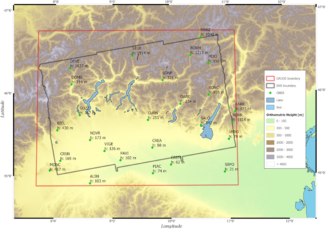
Figure 1. Map of the orography of the region. The gray rectangle indicates the footprint of the SAR observations, while the red rectangle is the area where GACOS data have been downloaded. The green dots indicate the GNSS stations with their code name and altitude, h.
2.2.1. GNSS ZTD Time Series
Dry air and water vapor molecules in the troposphere affect GNSS signals by lowering their propagation velocities with respect to vacuum (Saastamoinen, 1973; Bevis et al., 1992). A diminished speed results in a time delay in the signal propagation along the satellite-receiver path, which, multiplied by the vacuum speed of light, adds an extra distance to the satellite-receiver geometrical one. While from the positioning point of view this delay is just a systematic error to be removed, it enables the use of GNSS as a tool for the remote sensing of the troposphere water vapor content.
In this study only satellites of the GPS constellation are used. The dual-frequency observational files (RINEX Version 3 format), collected by 26 geodetic receivers (see Figure 1) of the SPIN network (Interregional Positioning Service for the Lombardia, Piemonte, and Valle D'Aosta regions, https://www.spingnss.it/), characterized by an interdistance or roughly 30–40 km, are processed with the goGPS software (Realini and Reguzzoni, 2013; Herrera et al., 2016). In particular, the goGPS software applies the PPP technique (Zumberge et al., 1997), by means of undifferenced phase observation processing, with precise products provided by International GNSS Service (IGS) and by applying ionosphere-free combination, to estimate both coordinates and ZTD values for each epoch by daily processing sessions.
ZTD is known to be the sum of a hydrostatic contribution, the Zenith Hydrostatic Delay or ZHD, and a wet contribution, the Zenith Wet Delay, which is related to the presence of water vapor (Bevis et al., 1992). The value of ZHD is basically the weight of the air column, i.e., the surface pressure (Saastamoinen, 1973), which has an exponential-like decay with height and is characterized by relatively small variations in time. ZWD, instead, is a highly turbulent field; it is very complex to model, and, even if it is one order of magnitude smaller than the ZHD, it is the most important term from a dynamical standpoint. As mentioned in the Introduction, ZWD is related to PWV. The conversion factor Π = PWV/ZWD depends on the vertical average of the inverse of the temperature weighted by the water vapor density and is roughly equal to 0.15 (Bevis et al., 1994). The goGPS software, after retrieving the ZTD, interpolates the ZHD from the gridded ZHD maps provided by the Vienna Mapping Function servers (Kouba, 2008) and get the ZWD as the difference ZWD = ZTD − ZHD. As a general remark, as the ZHD is much larger than the ZWD, the strong dependence of the ZHD on the height of the terrain is reflected in the ZTD field, as discussed in Fornaro et al. (2015).
In the time period of interest for this study (between January and November 2017), GNSS data are processed with goGPS to obtain a reference data set. To validate its reliability, a comparison test with atmospheric soundings was performed. Sounding balloons are extensively used in meteorological forecasting and research because they enable in situ recording of atmospheric variables with high temporal frequency and precision. The test was carried out in terms of ZTD and the results are in line with the literature with a standard deviation on ZTD differences of almost 1 cm (Mascitelli, 2020). Another validation test was performed with the radiometer. In particular, a pilot test was done comparing 1 year data from a four-channel Ka-band/W-band radiometer, located in the main campus of Politecnico di Milano, to the same data from a GNSS dual-frequency receiver (MILA), a part of a regional network and installed in the same campus, 280 m away from the radiometer. Also in this case, outputs were in line with literature, showing a standard deviation on PWV differences of almost 1.4 mm (Mascitelli, 2020).
Figure 2 shows the time series of the spatial statistics of both ZTD and ZWD of the 2017 data set. By looking at the spatial mean values of ZTD and ZWD (Figures 2A,C), it is evident that the ZTD seasonal cycle is due to the increased amount of water vapor that characterizes the summer season. In fact, the ZTD summer to winter difference is of the order of 150 mm, as shown in Figure 2A, which is the amplitude of the ZWD seasonal cycle, as in Figure 2C. Instead, by looking at the time series of the spatial standard deviation (Figures 2B,D), one can notice that the variability due to the presence of the orography is much larger than the variability of the water vapor field itself. In fact, the ZTD standard deviation is of the order of 160–170 mm, and the ZWD standard deviation is five times smaller. Only the ZWD standard deviation seems to have a seasonal cycle, which suggests that the summer increase in water vapor is not homogeneously distributed, also because the water vapor has a stratified component.
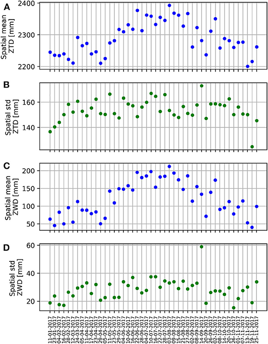
Figure 2. ZTD and ZWD spatial statistics as measured by the 26 GNSS stations of the SPIN network described in the main text. (A,B) are the mean and standard deviation of the ZTD; (C,D) for the ZWD. Note the different y-axis scales.
2.2.2. SAR APS Maps
SAR interferometry exploits the backscattering of the satellite radar electromagnetic signals by various targets on earth for various geodetic and remote sensing applications. In general, InSAR information is carried by the phase shift of the signal between subsequent passages over the same observed area. Since the atmospheric state affects the propagation of the radar signal, in particular with the presence of water vapor, InSAR observations can be used to map the ZTD over relatively large areas (Hanssen et al., 1999; Mateus et al., 2017).
SqueeSAR (Ferretti et al., 2011) is a state-of-the-art InSAR technique that is generally applied to estimate crustal deformations, and returns, as a by-product, APSs. It exploits information coming both from Permanent and Distributed Scatteres (PSs and DSs, respectively). PSs are relatively small objects that show a long phase stability over the observation period, such as rocks and man-made infrastructures. DSs instead cover larger areas and are stable over a shorter period of time (Ferretti et al., 2011; Manzoni et al., 2020). In order to properly estimate the crustal deformation effects, a large number of images is needed, making the algorithm quite computationally expensive.
To have a more detailed description of the algorithm, the reader is referred to the original work of Ferretti et al. (2011). Alternatively, one could read the works of Lagasio et al. (2019) and Manzoni et al. (2020), that briefly introduce the SqueeSAR algorithm because they make use of the same data set of the present work.
Forty-five APS maps are considered, starting from January 23 to November 25, 2017. During their processing, they all have January 11, 2017, as the master epoch and they are geo-referenced in a geographic WGS84 frame of reference, with grid spacing of roughly 90 m. Their footprint is shown in Figure 1 as a gray rectangle.
2.2.3. GACOS Maps
The acronym GACOS stands for Generic Atmospheric Correction Online Service. This service delivers high resolution ZTD maps aimed at the correction of atmospheric artifacts in InSAR products (Yu et al., 2017, 2018b). The high resolution ZTD maps, hereon referred to as GACOS model, are obtained by properly interpolating ZTD derived from the ECMWF atmospheric model at 0.125° and 6 h time resolution. Current products (such the ones used in the present paper) do not include observational ZTDs, although experiments using GNSS data have also been successfully performed (Yu et al., 2018a).
Here, the main characteristics of the Iterative Troposheric Decomposition (ITD) interpolation model used in GACOS are described. The ZTD of a generic ECMWF grid knot Pk is decomposed in a stratified component depending on the height of Pk plus a turbulent component depending on the considered position of Pk and a model error εk
The stratified component S(hk) is expressed in terms of an exponential height scaling function (Xu et al., 2011) depending on two unknown parameters S0 and β. These unknown parameters are estimated by applying an iterative procedure involving the ECMWF ZTD values falling in a given area (of the order of 100 km radius) surrounding the prediction point itself. The first estimate of the unknown parameters is done by performing a least squares adjustment of the ECMWF ZTD values in the area, modeled in terms of stratified components (the turbulent term is initially set to zero). The residuals between the ZTDs in the area and this first estimate of the stratified model are then removed from the original ZTDs. The residuals obtained in this step are used to predict the turbulent component on the ECMWF points themselves by applying an inverse distance weighting technique (e.g., Li et al., 2006). The obtained predicted turbulent components are then removed from the original ZTDs, obtaining new stratified values used for a new estimate of the unknown exponential model. The procedure is repeated until the unknown parameters converge to stable values. The final values of the stratified component and the turbulent ones are separately used to predict the ECMWF ZTDs onto the GACOS high resolution grid.
2.2.4. 3DVAR Maps
The Weather Research and Forecasting (WRF) model (Skamarock et al., 2008) is an NWP model that solves the non-hydrostatic fully compressible Euler equations using mass-based terrain-following coordinates. It is commonly used in research applications as well as in operational forecasting centers. In this work, its Data Assimilation package (Barker et al., 2012, WRFDA) has been used to generate ZTD maps at O (1 km) horizontal resolution to be interpreted as physically-based interpolations of the GNSS measurements. Figure 3 shows the numerical domains used for the NWP runs which have a grid spacing of 13.5, 4.5, and 1.5 km going from the largest to the smallest domain. Concerning the choice of the numerical parameterizations used in the WRF simulations, the reader is referred to Lagasio et al. (2019). An important aspect to be underlined is that to guarantee the numerical stability of the code, the orography used by the model is smoother that the realistic high-resolution Digital Elevation Model (DEM) associated to the SAR observations or to the real altitude measured by the GNSS stations. The differences can reach a few hundred meters and can, if not taken into account, result in ZTD discrepancies of the order of 10 cm, considering a surface atmospheric refractivity of about 300.
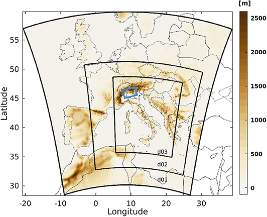
Figure 3. WRF model orography with the outline of the three numerical domains. From the outermost domain (d01) to the innermost one (d03) the grid spacing is 13.5, 4.5, and 1.5 km. The small light blue rectangle indicates the area covered by the SAR observations.
The 3DVAR maps shown here are based on simulations that are initialized at 1200UTC using the ECMWF-IFS fields (European Center for Medium-Range Weather Forecasts Integrated Forecasting System). Simulations are run for the SAR dates on the January 11, 2017, initially used as a master, and between April 11 and the July 4, 2017, for a total of 15 dates. The simulations run for 5 h, and at 17:00UTC, which corresponds to the time of the passage of Sentinel 1 above the area of interest (the precise time is 17:17UTC), the GNSS values are assimilated with WRFDA. To make sure that the numerical spinup that characterizes the first hours of every numerical simulation has faded out, the zonal wavenumber spectra of the horizontal wind components at 500 hPa are calculated. Then, following Skamarock (2004)'s approach, it has been checked that the spectra become steady at high wavenumber before the assimilation is performed, meaning that there are no numerical artifacts and the meteorological fields are realistic (not shown).
The 3DVAR assimilation technique (Bouttier and Courtier, 1999; Barker et al., 2012) aims at providing an optimal estimate of the atmospheric state using a previous estimate (coming, for example, from a forecast run or a global model) and a set of observations, weighted by their respective covariance error matrices. Mathematically, this is performed by minimizing the cost function of Equation (9) (Ide et al., 1997)
where x is the analysis to be found, xb is the first guess coming from the NWP model, y0 is the assimilated observation, and is the model-derived observation transformed from the analysis x by the observation operator for comparison against y0. The solution of (9) represents an a posteriori maximum likelihood estimate of the true state given the two sources of data (the first guess xb and the observation y0) weighted by the estimates of their errors. These are represented by B and R, which are the background error covariance matrix and the observation error covariance matrix, respectively. The R matrix contains error coming from the observational (i.e., instrumental) uncertainties and the representativity errors, which are introduced by the observation operator when manipulating the model data to be compared with the observations. In WRF 3DVAR, as in most of the assimilation systems (Bouttier and Courtier, 1999), R is diagonal, which assumes that the errors in the observations introduced by the various instruments are independent.
After performing the 3DVAR, the ZTD maps are calculated on the model grid by vertical integration of the atmospheric refractivity following Bevis et al. (1992), which is consistent with what is implemented in the WRF code. Finally, since there is a significant difference between the elevation of the DEM of the SAR measurements and the orography that WRF uses in the simulations, a correction to the ZTD is calculated as in Lagasio et al. (2019). In particular, when the model orography is higher than the GNSS station altitude, the modeled ZTD is underestimating the observed one, and a positive correction to the ZTD is added using the first model level refractivity and the height difference (remember that the ZTD is the vertical integral of the atmospheric refractivity). Instead, when the model orography is lower than the GNSS station height, the model is overestimating the observed ZTD and a negative correction is calculated by vertically integrating the model refractivity up to the GNSS station height.
3. Results
3.1. Accuracy Assessment on Differential ZTD
SAR calibrated differential maps are used to validate the time evolution of the atmospheric state simulated by the models under consideration. A comparison between the GNSS and the SAR observational products is performed as well. Note that the use of different wavelengths in the GNSS and SAR measurements, L-band and C-band, respectively, does not prevent their direct comparison for two reasons. Firstly, the troposphere is not dispersive for frequencies <30 GHz (Hanssen, 2001). Secondly, there is evidence in the literature that in case of simultaneous multi-frequency interferograms, the differential phases only show volumetric effects due to different penetration with frequency (Rosen et al., 1996). For the comparisons, ZTD values from GNSS, GACOS, and 3DVAR are therefore time differentiated using January 11, 2017, as the master epoch, while SAR maps are projected onto the zenith direction, obtaining the ΔZTD products defined in Equation (2).
The nearest neighbor method is used to coregister GACOS and SAR maps, whose spatial resolution is comparable. To account for the different spatial resolution of SAR and 3DVAR maps, SAR data are averaged and undersampled to the coarser 1.5 km grid of 3DVAR. The same procedure is applied whenever necessary. It is worth underlining that the goal of the present analysis is to validate each product at the maximum of its spatial resolution and time coverage, to assess its accuracy using SAR observations as a benchmark. Therefore, the sample size of the different products is kept as it is, unless a direct comparison between the GACOS and 3DVAR is performed. To this aim, we will denote with the star *, namely GACOS*, the GACOS maps undersampled over the 3DVAR grid. In the following analysis, it is considered only in the dates when the 3DVAR is available.
The following spatial and temporal statistics of model-SAR and GNSS-SAR time differential ΔZTDs are computed. Let x denote one of the products under consideration: GNSS, GACOS or 3DVAR. The spatial mean and standard deviation of the differences between differential ZTD products (k = 1, …, Lx is the spatial index) that change in time (i = 1…, Nx is the time index) are, respectively,
and
where the number of spatial points considered Lx changes for each product (GNSS, GACOS, and 3DVAR).
The time series of the statistics defined in the previous equations are displayed in Figure 4, the mean in Figure 4A and the standard deviation in Figure 4B. The GNSS-SAR average time series in Figure 4A is the result of the calibration procedure described in section 2.1. The GNSS-SAR standard deviation time series in Figure 4B shows a good agreement between the two techniques. The discrepancies, always below 15 mm, are due to the different observation techniques and modeling. Such discrepancies increase in summer, when more water vapor is present in the atmosphere and its turbulent component is more difficult to be estimated.
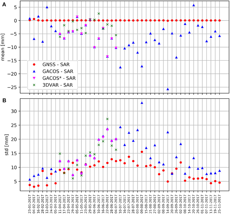
Figure 4. Time series of the spatial statistics of GNSS-SAR and model-SAR ΔZTD differences: mean values in (A) and standard deviation in (B).
GACOS shows to reproduce the spatial distribution of the SAR maps within the observational uncertainty from roughly October to May when the water vapor values are low. During summer and early fall, instead, when the atmosphere is moister, it has lower skills. It has a negative bias of O(5) mm, with standard deviations below 15 mm. The bias doubles in summer with an increase of the standard deviation to 25 mm.
In the dates where 3DVAR is available, its mean and standard deviation behavior follow GACOS ones. Note that the comparison between the two models is done after reducing the resolution of GACOS to that of 3DVAR. This change in resolution, however, has no significant impact in the comparison with SAR map (compare GACOS*-SAR with GACOS-SAR in Figure 4).
The temporal statistics for Lx points (k = 1, …, Lx) that evolve over Nx time steps (i = 1, …, Nx), for each x product (GNSS, GACOS, or 3DVAR) are calculated as
and
The above statistics are reported in Figure 5 for the GNSS-SAR comparison and in Figure 6 for the GACOS-SAR, GACOS*-SAR, and 3DVAR-SAR comparisons. The statistics are referred to the GNSS sparse locations, and to the original GACOS and 3DVAR grids.
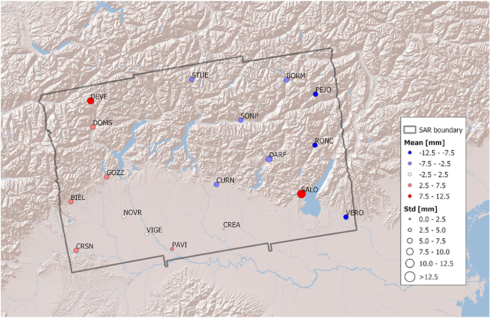
Figure 5. Map of the temporal statistics of the difference between GNSS ΔZTD values and SAR ΔZTD values.
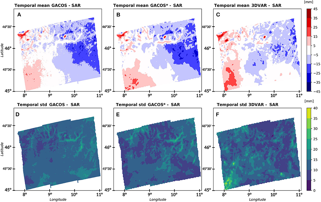
Figure 6. Map of the temporal statistics, mean and standard deviations, of the difference between the models ΔZTD maps and the SAR ΔZTD maps. (A,D) For GACOS at its original spatial resolution and using the entire data set; (B,E) for GACOS undersampled on the 3DVAR grid and considering only the dates where 3DVAR is available; (C,F) for 3DVAR.
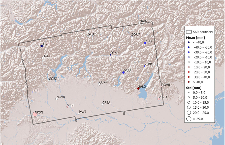
The temporal average of the GNSS-SAR ΔZTD differences is always below 15 mm (SALO has the largest bias of 12.5 mm, very likely because it is near a lake, which is known to introduce errors in the SAR observations), the largest biases in absolute value being in mountainous areas. There seems to be a large-scale trend, with zero spatial mean value, which is interpreted to be due to the different measuring algorithms of GNSS and SAR or to a systematic error contained in the SAR measurements, that depends on the master epoch of the observations. It also appears that in the plain the standard deviations are smaller than in the areas characterized by orography, which is reasonable because both GNSS and SAR are known to have issues in measuring tropospheric delays in such areas.
Figure 6 shows the maps of the temporal statistics calculated for the differences between the numerical models (GACOS and 3DVAR) ΔZTDs and the SAR ΔZTDs. Figures 6A,C show the mean difference of GACOS-SAR and 3DVAR-SAR, respectively, calculated at the full spatial resolution of the products and over the entire duration of the data sets. These two panels indicate that in mountainous areas there is a clear imprint of the orography and, in general, the model performances are worse than over the plain. Figure 6B is meant to be used to compare the two models: it shows the spatial mean GACOS*-SAR difference with GACOS undersampled over the 3DVAR grid and averaged on the same dates where the 3DVAR is available. Thus, comparing Figures 6B,C shows that GACOS have a larger temporal bias than 3DVAR, especially over the mountains in the eastern part of the domain, where there is a relatively large region with a bias lower than −15 mm. In general, we can say that in both products the bias in the mountainous region follows the spatial structure of the orography quite well, whereas the bias is much smoother over the plain. However, the values of the bias remain quite low (<15 mm) in most of the domain, meaning that even if the orography influences the spatial dependence of the temporal bias, it does not introduce a large systematic difference. In the middle of the domain, especially in the 3DVAR-SAR map in Figure 6C, one can see a blue area that corresponds to the relatively large urban area around the city of Milan. This bias can be interpreted with the fact that the WRF model was run with no urban physics parameterization, which lead to discrepancies in the surface fluxes and, thus, in the water vapor content and its time evolution. We argue that the large-scale residual of the averaged differences could be due to processing errors related to the master choice, such as phase signal unwrapping ambiguities, or the lack of estimation of systematic contributions, such as the ionospheric one. This aspect is not investigated in the present paper but could be a future development of this work.
Concerning the temporal standard deviation of the same ΔZTD differences, shown in Figures 6D–F, it is quite clear that, especially for GACOS, Figure 6D, the valleys are the place where the temporal variability of the difference is the highest. When looking at Figure 6E, GACOS*, and Figure 6F, 3DVAR, it is possible to directly compare the two products; it appears that they have the same range of variability. In the 3DVAR map there are some spatial features with high standard deviation, such as the tongue in the lower left corner of the domain or the bubble in the lower right corner, that can be recognized as instantaneous in some maps (not shown). This could be explained by the fact that the finer resolution over which the atmospheric dynamics is resolved in WRF with respect to GACOS leads to the representation of smaller and more intense atmospheric structures that, if they are misplaced in space or time, contribute to a larger deviation with respect to the observed SAR maps.
3.2. Accuracy Assessment on Absolute ZTD
After evaluating the performances of the models in the SAR observational space, we now compare directly the ZTD maps produced by GACOS and 3DVAR with the GNSS ZTD. The following statistics are used to evaluate the accuracy of the models in terms of differences with respect to our best observational product of the ZTD. In particular, we evaluate the spatial statistics of the differences (L being the number of the GNSS stations), namely the mean
the standard deviation
and the temporal statistics, the mean
and the standard deviation
Figure 7 shows the time series of the spatial statistics for GACOS, GACOS*, and 3DVAR. Looking at the year-long time series of the mean bias of GACOS in Figure 7A, one can see that there is an increase, in absolute value, in summer, of the same amplitude as the one observed in Figure 4A. August 9 and September 14 stand out for their bias larger than 15 mm (negative). The standard deviation, shown in Figure 7B also indicates that the models struggle more in representing the ZTD in summer, as previously highlighted.
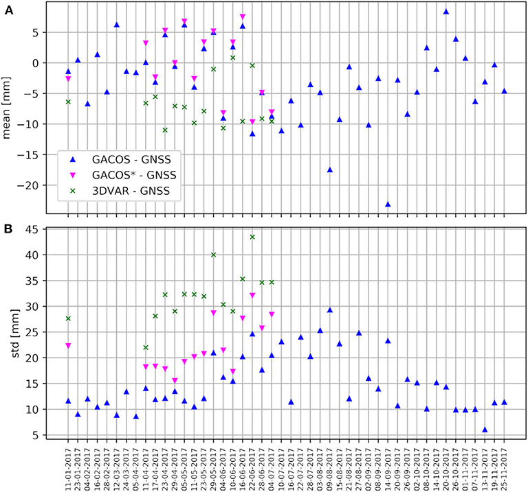
Figure 7. Time series of the spatial statistics of the differences between model ZTDs and GNSS ZTDs: mean values in (A) and standard deviation in (B).
The effect of decreasing the spatial resolution of the GACOS maps to 1.5 km grid spacing is visible when comparing the GACOS time series and the GACOS* one. It changes the mean value by about 1–2 mm, and the standard deviation by about 7–8 mm. The comparison between GACOS* and 3DVAR time series, then, highlights that the NWP model has a slightly larger bias, which is however always smaller than 15 mm, and a standard deviation that is roughly 1.5 times larger than the GACOS values.
The spatial variability of the differences of 3DVAR against GNSS doubles that of GACOS despite the fact that 3DVAR is assimilating the GNSS ZTD values. It is worth remarking that the 3DVAR model is corrected to account for the difference in height between the WRF DEM and the Shuttle Radar Topography Mission (SRTM) DEM, which is common to the GACOS model. To better interpret this discrepancy, it is insightful to look at the GACOS and 3DVAR ZTD dependence on the height, as displayed in Figure 8 for May 5, 2017. Figure 8A shows GACOS data and Figure 8B shows 3DVAR data. Both ZTD products have a strong dependence on the height, as expected from the definition of ZHD. However, for a given altitude, the spread of GACOS ZTD is much lower than the spread of 3DVAR ZTD. This is linked to how the small scale variability is handled in the two models: GACOS method produces a ZTD with a strong dependence on the height, while 3DVAR solves the atmospheric equations of motion over a smoothed orography and makes use of parameterizations to account for the sub-grid scale phenomena, such as turbulence. If one takes the range (maximum–minimum) of ZTD values at a given height, an estimate of the spatial standard deviation is given by dividing the range by six, assuming a normal distribution. For instance, for the reference height of 2,000 m, the standard deviation of the ZTD is roughly 25 mm for GACOS ZTD and 65 mm for 3DVAR, more than the double. This higher spatial variability of the ZTD modeled by 3DVAR, associated with the fact that the water vapor turbulent fluctuations cannot be well-estimated by the point-wise and averaged GNSS ZTD explains why the spatial standard deviation of the 3DVAR ZTD-GNSS ZTD difference is larger than the standard deviation of the GACOS ZTD-GNSS ZTD.
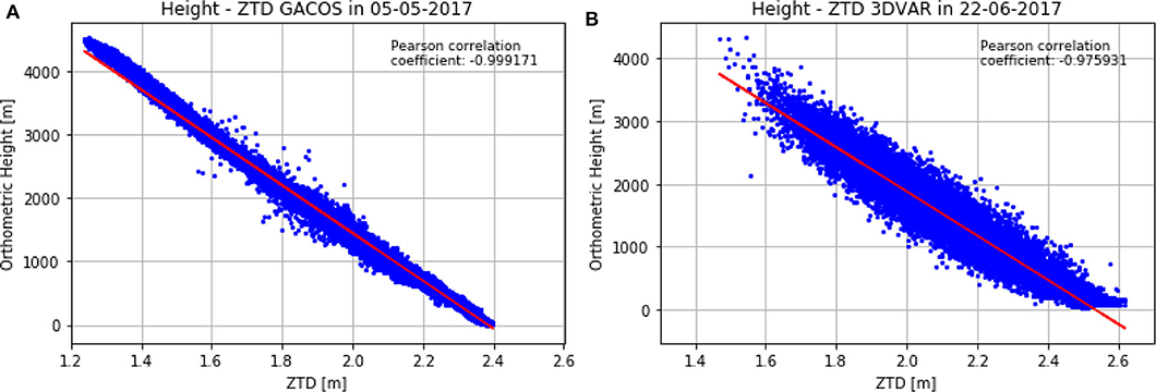
Figure 8. Scatterplot of the GACOS ZTD values and the InSAR DEM height (A) as well as of the 3DVAR ZTD values and the WRF model height (B).
A confirmation of this comes from further analysis that evaluate the relative role of the GNSS assimilation in the NWP model and the height correction introduced at the end of section 2.2.4, which accounts for the height discrepancy between the model orography and the real terrain using the modeled refractivity. In particular, Figure 9 shows the spatial statistics calculated on three more data sets:
• the outputs of the WRF model before performing the GNSS assimilation and with no correction of the height difference between model and InSAR DEM, named “WRFNC” in the figure;
• the WRF outputs with no data assimilation but with the height difference correction, named “WRF”;
• the WRFDA outputs with no height correction, named “3DVARNC.”
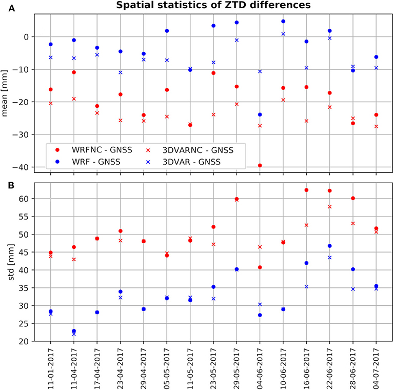
Figure 9. Spatial statistics of the ZTD differences with respect to the GNSS ZTD. The time series of the mean value are shown in (A) and the time series of the standard deviation are shown in (B). “WRFNC” indicates the model outputs with no data assimilation and no height correction; “WRF” are the outputs of WRF corrected for the height difference with the InSAR data; “3DVARNC” shows the model output after assimilating the GNSS with no height discrepancy correction; “3DVAR” denotes the time series of the 3DVAR output corrected for the height difference.
The fourth time series shown in the figure comes from the 3DVAR output that have been corrected for the height difference, as shown in Figure 7.
Figure 9A shows that the correction due to height discrepancy between the WRF and InSAR DEM, that was described at the end of section 2.2.4, clearly improves the modeled ZTD with respect to GNSS by an amount of 10–15 mm, in both the 3DVAR and WRF cases. As the height correction is not homogeneously applied to all the points (the largest discrepancies between WRF and InSAR DEM are in fact located in the mountainous areas), the spatial variability of the ZTD differences of non-corrected models is higher than that of the corrected ones, as is clearly shown in Figure 9B. The statistics of WRF-GNSS and 3DVAR-GNSS are not significantly different.
Figures 10–12 show the map of the temporal statistics of the difference between GACOS ZTD-GNSS ZTD, GACOS* ZTD-GNSS ZTD, and 3DVAR ZTD-GNSS ZTD, respectively. Again, GACOS has a good agreement with GNSS ZTDs, the majority of stations having a mean absolute difference below 10 mm and a standard deviation below 15 mm. In comparison with 3DVAR, made on the reduced GACOS*, it behaves similarly everywhere, except for few stations in the mountain regions, where it performs slightly worse. Both 3DVAR and GACOS temporal means are generally negative over the mountains and positive over the plain.
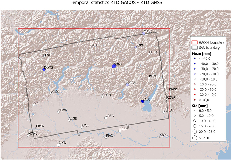
Figure 10. Map of the temporal statistics of the difference between GACOS ZTD and GNSS ZTD. In this figure, GACOS has been taken with its original spatial resolution and for all 46 dates.
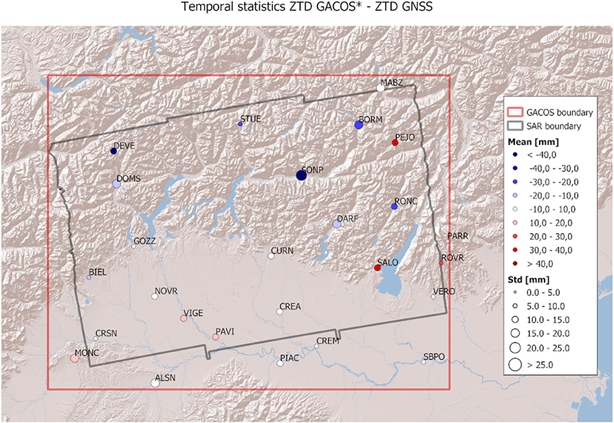
Figure 11. Map of the temporal statistics of the difference between GACOS* ZTD and GNSS ZTD. Note that here, the statistics for GACOS are computed after undersampling it on the 3DVAR grid and only on the 14 dates where 3DVAR is available.
3.3. Impacts of the Master Retrieval Strategy on SAR ZTD Maps
An assessment of the accuracy of the final SAR ZTD maps, either obtained by adding a single master map from an external product or by adding a master TAE, as in Equation (5), is now performed. Only the GACOS data set is used, both because it covers the entire year and because it has been shown to be more accurate than the 3DVAR data set.
It is worth remarking that, in what follows, we change the master time of a stack of ΔZTD(Pk, tj, tM) maps referred to the master epoch tM. This is done by removing from all the maps the ΔZTD(Pk, ti, tM) of the new master ti with respect to the current one, namely
This means that, when using the TAE approach with a single master (N = 1), if the new master epoch ti is different from the original master epoch tM, we are simply changing the master epoch so that, instead of having
which would be the standard single master epoch approach, we have
even if the ΔZTD were originally referred to the tM epoch. Note that here we explicitly write the dependence of the SAR ZTD on the master ti as we study how different choices of the master affect the resulting absolute map. In the TAE approach, the final SAR ZTD map at the slave epoch tj does not depend on the initial master epoch tM, but only on ti or, in the case of N > 1, on all the epochs used in the time average ti, i = 1, …, N.
In the case of TAE with N > 1, the SAR ZTD is
where is the SAR ZTD obtained with a single master map ti, as introduced in Equation (20). This shows that the TAE approach is equivalent to averaging in time the SAR ZTD obtained using all the epochs ti, i = 1, …, N as master epochs.
The spatial bias of the final SAR ZTD maps for N > 1, with respect to the GNSS ZTD, writes
where we exploit (21) to express it as the temporal mean of the spatial biases of the SAR ZTD maps with N = 1 in the time interval of interest.
The bias of the SAR ZTD at the slave epoch tj for N = 1 with ti as the master epoch can be written as
The first term is the spatial bias of the modeled ZTD with respect to the GNSS ZTD at the slave epoch tj, , as defined in Equation (14). This, as Figure 7 shows, has a seasonal cycle with the poorest performances in summer, as discussed in section 3.2. However, also the second term, which is the spatial bias of the modeled ΔZTD with respect to the SAR ΔZTD, has a similar seasonal cycle with similar values (see section 3.1). Figure 4, in particular, shows this spatial bias, defined in Equation (10), with ti equal to the 11 January 2017, which is the original master epoch of the data set. Thus, for a given master epoch ti, the quantity is the difference between two terms that have a similar seasonal cycle and that roughly compensate themselves on this temporal scales. For a given master ti, the SAR ZTD bias is, then, almost constant throughout the year with respect to the slave epoch tj. This is clearly shown by Figure 13, where is plotted for the entire GACOS data set.
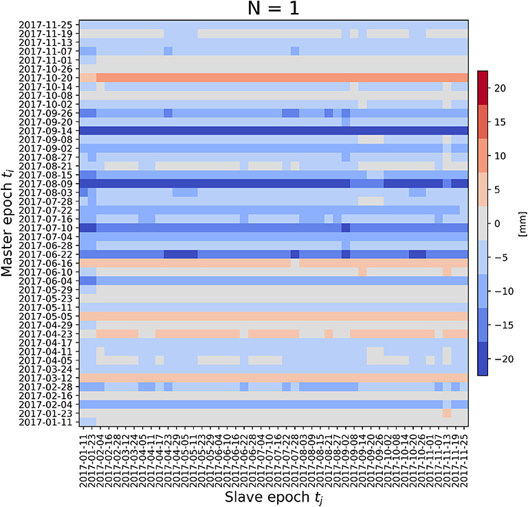
Figure 13. SAR ZTD bias with a single master epoch , as defined in Equation (23), calculated for the entire GACOS data set.
Concerning the dependence of the SAR ZTD bias on the master epoch ti, instead, Equation (23) shows that only the second term, the bias of the modeled ΔZTD, depends on it. This suggests that a seasonal cycle is expected because there cannot be a compensation. In fact, note that the ΔZTD is anti-symmetric with respect to the master and slave epoch choice, namely
by its definition. This means that, for any fixed slave tj, the dependence of the SAR ZTD bias on the master ti has the functional form of
meaning that the minimum is attained in summer, as shown, again, in Figure 4. This is also visible in Figure 13, which proves that the ti master epoch choice is what really determines the bias of the final SAR ZTD maps. In particular, the summer master epoch generally introduces a larger bias with respect to epochs chosen in other seasons.
For N > 1, replacing Equation (23) in Equation (22) one gets that the SAR ZTD bias is given by the difference of the bias of the modeled ZTD (with respect to the GNSS ZTD) and the time average of the bias of the modeled ΔZTD (with respect to SAR ΔZTD), namely
Thus, the dependence on the ti, i, …, N master epochs is explicitly on the time average of their bias. For sake of simplicity, we calculate , the time average of the SAR ZTD single-master bias, using a running mean of N master epochs. The SAR ZTD bias is shown in Figure 14 as a function of tj, the slave epoch, and ti, the central master epoch of the sliding window (with N = 3 in Figure 14A and N = 11 in Figure 14B), calculated for the entire GACOS data set. Note that the initial and final (N − 1)/2 values of ti are missing, because of the width of the sliding window. However, remind that one could arbitrarily choose the master epochs over which to calculate the time average.
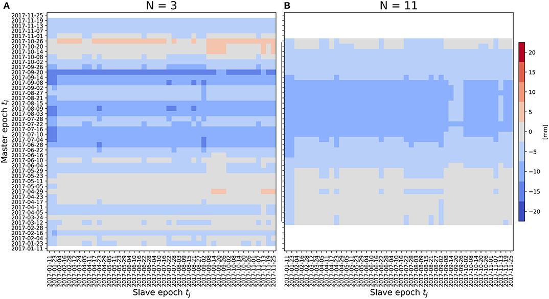
Figure 14. SAR ZTD bias with a N = 3 (A) and N = 11 (B) master epochs , as defined in Equation (22), calculated for the entire GACOS data set. A sliding window centered on the ti epochs is used.
Figure 14 shows that also for N > 1, the dependence of the bias on the slave epoch tj is much weaker than on the master epochs ti, i = 1, …, N. Moreover, it is confirmed that even with the TAE approach summer master epochs introduce a larger bias and should be avoided. In particular, this suggests that in the limit of using all the maps available for time averaging, the resulting bias is larger than the bias obtained by choosing a single (or few) master epoch(s) in late fall, winter, or spring. This happens because the seasonality of the ΔZTD bias has a non-zero average value, and, thus, it is more convenient to average on a subset of master epochs with a small bias (typically avoiding summer epochs), than to consider all of them.
To summarize, as there is a seasonal behavior in the ΔZTD bias, which propagates to the SAR ZTD bias through the choice of the ti master epoch, the accuracy of the final ZTD maps depends on the dates chosen in the TAE approach (even in the case of a single master epoch, N = 1). Thus, the dates have to be chosen when the model performances are good, which has been shown to happen when there is a little amount of water vapor. Even if in the present section only GACOS was used; note that the equations apply for any modeled ZTD product used as an external source. In particular, similar conclusions could be drawn for 3DVAR because a very similar seasonal behavior, with evidence of poor performances of the model during summer, is observed.
4. Conclusions
A systematic comparison of various methods to obtain absolute ZTD maps from InSAR APS has been performed. In particular, the online product GACOS and the outputs of a data assimilation package of a state-of-the-art NWP model have been validated with respect to SAR and GNSS observations and have been compared to each other. The master map was obtained both by taking a single image from the two products (GACOS and 3DVAR), and by taking a time average of these products and the corresponding APS maps following the approach introduced by Pichelli et al. (2015).
A first result is that, in terms of the NWP products, the assimilation of ZTD GNSS observations introduces a smaller variation with respect to the correction due to the height difference between the numerical model orography and the fine-scale InSAR DEM. This is unavoidable because the NWP model needs to solve the equations of motion on a smoother orography for numerical stability constraints. Moreover, NWP models use parameterizations to take into account sub-grid scale phenomena, such as turbulence. These two aspects lead to the conclusion that the fine-scale spatial features of the water vapor field cannot be captured by the NWP models to a degree of accuracy higher than a simpler iterative method, such as the one implemented in GACOS, where the ZTD dependence on the height is stronger. Thus, it is not worth implementing the 3DVAR approach to derive the master map because it is more numerically Demanding.
The analysis of the SAR ZTD bias as a function of the slave and master epochs, both using a single master epoch or a time average of them, suggest that it is crucial to choose a reliable master map (or a set of them), meaning that it compares (they compare) well with GNSS, which is a reference measurement of the absolute ZTD. In fact, if the master has a large bias with respect to the observations, this uncertainty propagates to all the absolute ZTD maps derived. Moreover, time averaging external ZTD maps and the corresponding APSs does not guarantee that the master is better, as, if the instants included in the estimate have a large bias, the resulting master map will also be significantly different from the observations. Care must be taken in summer, where the models have more difficulty in reproducing the water vapor spatial distribution. Additionally, mountainous areas are characterized by larger biases, and, thus, if they are included in the region of interest, they contribute to a larger uncertainty in final absolute ZTD maps.
Finally, the present work shows some metrics that can be useful to assess the uncertainty associated to the InSAR-derived absolute maps. This is an important aspect for data assimilation experiments, which are one of the most promising applications of such novel high-resolution products.
Data Availability Statement
The GACOS data sets analyzed for this study can be downloaded at: https://research.ncl.ac.uk/. The WRF and 3DVAR data supporting the conclusions of this article will be made available by the authors, without undue reservation. The SAR APS data analyzed in this study were obtained from T.R.E. Altamira company, using their proprietary software, SqueeSAR. Their access, thus, is restricted. Requests to access these datasets should be directed to Alessio Rucci (YWxlc3Npby5ydWNjaUB0cmUtYWx0YW1pcmEuY29t).
Author Contributions
GV and AM-G carried out the conceptualization. GV and ANM were responsible for the methodology, preparation, and writing of the original draft. SB, MMo, and ANM carried out the formal analysis. AM, MMa, MMo, ER, GT, AG, SB, ML, and ANM carried out the data curation. GV, AM, and ANM wrote, reviewed, and edited the manuscript. MMo was responsible for the visualization. GV, AM-G, ER, and AP were responsible for supervision and carried out the funding acquisition. All authors have read and agreed to the published version of the manuscript.
Funding
This work was partially funded by TWIGA. The TWIGA project has received funding from the European Union's Horizon 2020 Research and Innovation Programme under grant agreement no. 776691. MMo and partially AM were supported by Fondazione Cariplo within the project: Lombardy-based Advanced Meteorological Predictions and Observations (LAMPO) (2017-0725).
Conflict of Interest
AG, ER, and GT are employed by the company Geomatics Research and Development (GReD) s.r.l.
The remaining authors declare that the research was conducted in the absence of any commercial or financial relationships that could be construed as a potential conflict of interest.
Acknowledgments
The authors would like to thank the entire TRE Altamira team for the SqueeSAR stack of images.
References
Barindelli, S., Realini, E., Venuti, G., Fermi, A., and Gatti, A. (2018). Detection of water vapor time variations associated with heavy rain in northern Italy by geodetic and low-cost GNSS receivers. Earth Planets Space 70:28. doi: 10.1186/s40623-018-0795-7
Barker, D., Huang, X.-Y., Liu, Z., Auligné, T., Zhang, X., Rugg, S., et al. (2012). The Weather Research and Forecasting model's community variational/ensemble data assimilation system: WRFDA. Bull. Am. Meteor. Soc. 93, 831–843. doi: 10.1175/BAMS-D-11-00167.1
Berardino, P., Fornaro, G., Lanari, R., and Sansosti, E. (2002). A new algorithm for surface deformation monitoring based on small baseline differential SAR interferogram. IEEE Trans. Geosci. Rem. Sens. 40, 2375–2382. doi: 10.1109/TGRS.2002.803792
Bevis, M., Businger, S., Chiswell, S., Herring, T. A., Anthes, R. A., Rocken, C., et al. (1994). GPS meteorology: mapping zenith wet delays onto precipitable water. J. Appl. Meteorol. 33, 379–386. doi: 10.1175/1520-0450(1994)033<0379:GMMZWD>2.0.CO;2
Bevis, M., Businger, S., Herring, T. A., Rocken, C., Anthes, R. A., and Ware, R. H. (1992). GPS meteorology: remote sensing of atmospheric water vapor using the global positioning system. J. Geophys. Res. 97, 15787–15801. doi: 10.1029/92JD01517
Bouttier, F., and Courtier, P. (1999). Data Assimilation Concepts and Methods. Meteorological Training Course Lecture Series. Reading: ECMWF.
Ferretti, A., Fumagalli, A., Novali, F., Prati, C., Rocca, F., and Rucci, A. (2011). A new algorithm for processing interferometric data-stacks: Squeesar. IEEE Trans. Geosci. Rem. Sens. 49, 3460–3470. doi: 10.1109/TGRS.2011.2124465
Ferretti, A., Prati, C., and Rocca, F. (1999). “Permanent scatterers in SAR interferometry,” in IEEE 1999 International Geoscience and Remote Sensing Symposium (Hamburg), 1528–1530. doi: 10.1109/IGARSS.1999.772008
Fornaro, G., D'Agostino, N., Giuliani, R., Noviello, C., Reale, D., and Verde, S. (2015). Assimilation of GPS-derived atmospheric propagation delay in DInSAR data processing. IEEE J. Sel. Top. Appl. Earth Obs. Rem. Sens. 8, 784–799. doi: 10.1109/JSTARS.2014.2364683
Hanssen, R. F. (2001). Radar Interferometry: Data Interpretation and Error Analysis. Dordrecht: Kluwer Academic Publishers.
Hanssen, R. F., Weckwerth, T. M., Zebker, H. A., and Klees, R. (1999). High-resolution water vapor mapping from interferometric radar measurements. Science 283, 1297–1299. doi: 10.1126/science.283.5406.1297
Hdidou, F. Z., Mordane, S., Moll, P., Mahfouf, J. F., Erraji, H., and Dahmane, Z. (2020). Impact of the variational assimilation of ground-based GNSS zenith total delay into AROME-Morocco model. Tellus A 72, 1–13. doi: 10.1080/16000870.2019.1707854
Herrera, A. M., Suhandri, H. F., Realini, E., Reguzzoni, M., and de Lacy, M. C. (2016). goGPS: open-source MATLAB software. GPS Solut. 20, 595–603. doi: 10.1007/s10291-015-0469-x
Ide, K., Courtier, P., Ghil, M., and Lorenc, A. C. (1997). Unified notation for data assimilation: operational, sequential and variational. J. Meteorol. Soc. Jpn. 75, 181–189. doi: 10.2151/jmsj1965.75.1B_181
Kouba, J. (2008). Implementation and testing of the gridded Vienna Mapping Function 1 (VMF1). J. Geod. 82, 193–205. doi: 10.1007/s00190-007-0170-0
Lagasio, M., Parodi, A., Pulvirenti, L., Meroni, A. N., Boni, G., Pierdicca, N., et al. (2019). A synergistic use of a high-resolution numerical weather prediction model and high-resolution Earth observation products to improve precipitation forecast. Rem. Sens. 11:2387. doi: 10.3390/rs11202387
Li, Z., Fielding, E. J., Cross, P., and Muller, J. P. (2006). Interferometric synthetic aperture radar atmospheric correction: GPS topography-dependent turbulence model. J. Geophys. Res. Solid Earth 111:B02404. doi: 10.1029/2005JB003711
Manzoni, M., Monti Guarnieri, A. V., Realini, E., and Venuti, G. (2020). Joint exploitation of SAR and GNSS for atmospheric phase screens retrieval aimed at numerical weather prediction model ingestion. Rem. Sens. 12:654. doi: 10.3390/rs12040654
Mascitelli, A. (2020). New applications and opportunities of GNSS meteorology (Ph.D. thesis), Rome: Sapienza University of Rome.
Mascitelli, A., Federico, S., Fortunato, M., Avolio, E., Torcasio, R. C., Realini, E., et al. (2019). Data assimilation of GPS-ZTD into the RAMS model through 3D-Var: preliminary results at the regional scale. Meas. Sci. Technol. 30:055801. doi: 10.1088/1361-6501/ab0b87
Mateus, P., Catalão, J., and Nico, G. (2017). Sentinel-1 interferometric SAR mapping of precipitable water vapor over a country-spanning area. IEEE Trans. Geosci. Rem. Sens. 55, 2993–2999. doi: 10.1109/TGRS.2017.2658342
Mateus, P., Miranda, P., Nico, G., Catalão, J., Pinto, P., and Tomé, R. (2018). Assimilating InSAR maps of water vapor to improve heavy rainfall forecasts: a case study with two successive storms. J. Geophys. Res. Atmos. 123, 3341–3355. doi: 10.1002/2017JD027472
Mateus, P., Tomé, R., Nico, G., and Catalão, J. (2016). Three-dimensional variational assimilation of InSAR PWV using the WRFDA model. IEEE Trans. Geosci. Rem. Sens. 54, 7323–7330. doi: 10.1109/TGRS.2016.2599219
Miranda, P., Mateus, P., Nico, G., Catalão, J., Tomé, R., and Nogueira, M. (2019). Insar meteorology: high-resolution geodetic data can increase atmospheric predictability. Geophys. Res. Lett. 46, 2949–2955. doi: 10.1029/2018GL081336
Monti Guarnieri, A., Leanza, A., Recchia, A., Tebaldini, S., and Venuti, G. (2018). Atmospheric phase screen in GEO-SAR: estimation and compensation. IEEE Trans. Geosci. Rem. Sens. 56, 1668–1679. doi: 10.1109/TGRS.2017.2766084
Monti Guarnieri, A., and Rocca, F. (2017). Options for continuous radar Earth observations. Sci. China Inform. Sci. 60:060301. doi: 10.1007/s11432-016-9067-7
Oigawa, M., Realini, E., Seko, H., and Tsuda, T. (2014). Numerical simulation on retrieval of meso-γ scale precipitable water vapor distribution with the Quasi-Zenith Satellite System (QZSS). J. Meteorol. Soc. Jpn. 92, 189–205. doi: 10.2151/jmsj.2014-301
Oigawa, M., Tsuda, T., Seko, H., Shoji, Y., and Realini, E. (2018). Data assimilation experiment of precipitable water vapor observed by a hyper-dense GNSS receiver network using a nested NHM-LETKF system. Earth Planets Space 70:74. doi: 10.1186/s40623-018-0851-3
Pepe, A., Sansosti, E., Berardino, P., and Lanari, R. (2005). On the generation of ERS/ENVISAT DInSAR time-series via the sbas technique. IEEE Geosci. Rem. Sens. Lett. 2, 265–269. doi: 10.1109/LGRS.2005.848497
Pichelli, E., Ferretti, R., Cimini, D., Panegrossi, G., Perissin, D., Pierdicca, N., et al. (2015). InSAR water vapor data assimilation into mesoscale model MM5, Technique and pilot study. IEEE J. Sel. Top. Appl. Earth Obs. Rem. Sens. 8, 3859–3875. doi: 10.1109/JSTARS.2014.2357685
Pierdicca, N., Maiello, I., Sansosti, E., Venuti, G., Ferretti, R., Gatti, A., et al. (2020). Excess path delays from Sentinel-1 interferometry to improve weather forecasts. IEEE J. Sel. Top. Appl. Earth Obs. Rem. Sens. 13, 3213–3228. doi: 10.1109/JSTARS.2020.2988724
Realini, E., and Reguzzoni, M. (2013). goGPS: Open source software for enhancing the accuracy of low-cost receivers by single-frequency relative kinematic positioning. Meas. Sci. Technol. 24:115010. doi: 10.1088/0957-0233/24/11/115010
Rosen, P., Hensley, S., Zebker, H. A., Webb, F., and Fielding, E. (1996). Surface deformation and coherence measurements of Kilauea Volcano, Hawaii, from SIR-C radar interferometry. J. Geophys. Res. 101, 23109–23125. doi: 10.1029/96JE01459
Ruiz Rodon, J., Broquetas, A., Monti Guarnieri, A., and Rocca, F. (2013). Geosynchronous SAR focusing with atmospheric phase screen retrieval and compensation. IEEE Trans. Geosci. Rem. Sens. 51, 4397–4404. doi: 10.1109/TGRS.2013.2242202
Saastamoinen, J. (1973). Contributions to the theory of atmospheric refraction. Bull. Good. 107, 13–14. doi: 10.1007/BF02522083
Sherwood, S. C., Roca, R., Weckwerth, T. M., and Andronova, N. G. (2010). Tropospheric water vapor, convection and climate. Rev. Geophys. 48, RG2001. doi: 10.1029/2009RG000301
Shoji, Y. (2013). Retrieval of water vapor inhomogeneity using the Japanese nationwide GPS array and its potential for prediction of convective precipitation. J. Meteorol. Soc. Jpn. 91, 43–62. doi: 10.2151/jmsj.2013-103
Skamarock, W. C. (2004). Evaluating mesoscale NWP models using kinetic energy spectra. Mon. Weather Rev. 132, 3019–3032. doi: 10.1175/MWR2830.1
Skamarock, W. C., Klemp, J. B., Dudhia, J., Gill, D. O., Barker, D. M., Duda, M. G., et al. (2008). A Description of the Advanced Research WRF Version 3. NCAR Tech. Note NCAR/TN-475+STR, Boulder, CO: National Center for Atmospheric Research (NCAR), 113.
Tang, X., Sun, J., Zhang, Y., and Tong, W. (2019). Constraining the large0scale analysis of a regional rapid-update-cycle system for short-term convective precipitation forecasting. J. Geophys. Res. Atmos. 124, 6949–6965. doi: 10.1029/2018JD030190
Xu, W. B., Li, Z. W., Ding, X. L., and Zhu, J. J. (2011). Interpolating atmospheric water vapor delay by incorporating terrain elevation information. J. Geod. 85, 555–564. doi: 10.1007/s00190-011-0456-0
Yang, S. C., Huang, Z. M., Huang, C. Y., Tsai, C. C., and Yeh, T. K. (2020). A case study on the impact of ensemble data assimilation with GNSS-Zenith total delay and radar data on heavy rainfall prediction. Mon. Weather Rev. 148, 1075–1098. doi: 10.1175/MWR-D-18-0418.1
Yu, C., Li, Z., and Penna, N. T. (2018a). Interferometric synthetic aperture radar atmospheric correction using a GPS-based iterative tropospheric decomposition model. Rem. Sens. Environ. 204, 109–121. doi: 10.1016/j.rse.2017.10.038
Yu, C., Li, Z., Penna, N. T., and Crippa, P. (2018b). Generic atmospheric correction model for interferometric synthetic aperture radar observations. J. Geophys. Res. Solid Earth 203, 9202–9222. doi: 10.1029/2017JB015305
Yu, C., Penna, N. T., and Li, Z. (2017). Generation of real-time mode high-resolution water vapor fields from gps observations. J. Geophys. Res. Atmos. 122, 2008–2025. doi: 10.1002/2016JD025753
Keywords: water vapor, GNSS meteorology, SAR meteorology, master estimate, numerical weather prediction, ZTD, APS, data assimilation
Citation: Meroni AN, Montrasio M, Venuti G, Barindelli S, Mascitelli A, Manzoni M, Monti-Guarnieri AV, Gatti A, Lagasio M, Parodi A, Realini E and Tagliaferro G (2020) On the Definition of the Strategy to Obtain Absolute InSAR Zenith Total Delay Maps for Meteorological Applications. Front. Earth Sci. 8:359. doi: 10.3389/feart.2020.00359
Received: 06 April 2020; Accepted: 04 August 2020;
Published: 26 October 2020.
Edited by:
Giovanni Nico, Istituto per le Applicazioni del Calcolo “Mauro Picone” (IAC), ItalyReviewed by:
Mukesh Gupta, Catholic University of Louvain, BelgiumGianfranco Fornaro, National Research Council (CNR), Italy
Copyright © 2020 Meroni, Montrasio, Venuti, Barindelli, Mascitelli, Manzoni, Monti-Guarnieri, Gatti, Lagasio, Parodi, Realini and Tagliaferro. This is an open-access article distributed under the terms of the Creative Commons Attribution License (CC BY). The use, distribution or reproduction in other forums is permitted, provided the original author(s) and the copyright owner(s) are credited and that the original publication in this journal is cited, in accordance with accepted academic practice. No use, distribution or reproduction is permitted which does not comply with these terms.
*Correspondence: Agostino N. Meroni, YWdvc3Rpbm8ubWVyb25pQGdtYWlsLmNvbQ==
 Agostino N. Meroni
 Marco Montrasio
 Giovanna Venuti
 Stefano Barindelli
 Alessandra Mascitelli
 Marco Manzoni
 Andrea V. Monti-Guarnieri3
 Andrea Gatti
 Martina Lagasio
 Eugenio Realini