Asynchronous Hydroclimatic Modeling for the Construction of Physically Based Streamflow Projections in a Context of Observation Scarcity

Asynchronous hydroclimatic modeling is proposed for the construction of physically based streamflow projections over regions characterized by meteorological observation scarcity. The novel approach circumvents the requirement for meteorological observations by 1) calibrating quantile mapping transfer functions simultaneously to the parameters of the hydrologic model, 2) forcing the hydrologic model with post-processed climate simulations, and 3) intentionally ignoring the correlation between simulated streamflow values and observations. As a result, relative humidity, solar radiation and wind speed are integrated to a full hydroclimatic modeling chain, allowing the construction of streamflow projections forcing the Penman-Montheith reference evapotranspiration formulation over a forested catchment that flows into the St-Lawrence River, Canada. Results confirm a more accurate simulated hydrological response relative to a conventional hydroclimatic modeling chain employing reanalyses as description of the climate system. They also highlight the contribution to uncertainty in streamflow projections from biased climate variables issued by the reanalyses. The suggested framework assumes the hydrologic regime as a functional proxy to corresponding climate drivers. We believe the latter opens promising perspectives in the scope of producing more reliable estimations of water-related and energy-driven processes such as streamflow generation, snow accumulation and melt, river ice jams, water temperature, or vegetation growth under evolving climate conditions.

Introduction

The analysis of climate change impacts on water resources commonly involves a hydroclimatic modeling chain (Muerth et al., 2013; Ott et al., 2013; Arheimer and Lindström, 2015), with components including climate simulations from global or regional climate models (GCMs or RCMs), statistical post-processing of these simulations, and hydrologic modeling using post-processed simulations as inputs and projecting perturbations of the hydrologic regime at the catchment scale. Using climate scenarios as inputs, hydrologic models simulate streamflow at a given catchment outlet by reproducing water-related processes such as evapotranspiration, snow accumulation and melt, soil water content fluctuations, and routing within the river network (e.g., Najafi et al., 2011; Teutschbein et al., 2015).

Hydrologic models can be categorized on how processes are represented. On the one hand, conceptual models favor the usage of simpler empirical formulations, estimating hydrologic processes with available climate drivers, generally air temperature and precipitation. On the other hand, physically based models rely on a more exhaustive integration of fundamental laws of physics such as mass and energy conservations. Since laws of physics are not expected to be affected by climate change, physically based models are assumed, at least from a theoretical perspective, to provide more reliable streamflow projections (Lofgren et al., 2013; Shaw and Riha, 2011; Feng et al., 2017). Recent works confirm the sensitivity of streamflow projections to the structure of hydrologic models (Velázquez et al., 2013; Dams et al., 2015; Seiller and Anctil, 2016).

Figure 1A schematizes the construction of streamflow projections resorting to a conventional configuration of the hydroclimatic modeling chain. Typically, a statistical post-processing (here quantile mapping) is applied to a raw climate simulation when it differs from a trusted reference product (ideally high-quality meteorological observations) over a period long enough to encompass local climate variability (Maraun et al., 2017). A transfer function is defined by comparing the raw climate simulation to corresponding meteorological observations over a calibration period generally set within the reference period of the climate model, namely the time interval corresponding to a simulated recent past. A post-processed climate simulation is subsequently constructed by applying the transfer function to the raw climate simulation over a given application period, generally including both reference and future periods simulated by the climate model. Independently, a hydrologic model is calibrated in order to minimize errors between observed and simulated streamflow at the catchment outlet. The latter model is forced with meteorological observations while the optimization algorithm iteratively searches for an optimal set of free parameters according to a selected objective function. Streamflow projections are finally constructed by forcing the calibrated hydrologic model with post-processed climate simulations.

FIGURE 1

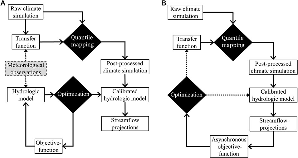
FIGURE 1. (A) A conventional configuration of the hydroclimatic modeling chain. (B) The suggested asynchronous configuration circumventing the requirement for meteorological observations.

Within a conventional hydroclimatic modeling framework, the construction of streamflow projections using physically based hydrologic models is often limited by the lack of meteorological observations. Quantile mapping and calibration of the hydrologic model both require meteorological observations (Figure 1A, dashed lines), the former for defining transfer functions, the latter for forcing the hydrologic model while calibrating its parameters. The most prevalent hydroclimatic modeling chain reported in the literature exclusively considers air temperature and precipitation as inputs, thus employing empirical representations of the hydrologic processes (Das et al., 2013; Tramblay et al., 2014; Rössler et al., 2019). Additional climate drivers such as relative humidity, solar radiation, and wind speed (hereafter referred to as HRW variables) are required when evaluating energy-based representations of the hydrologic processes like the Penmann-Montheith reference evapotranspiration formulation (Kay et al., 2013; Boulard et al., 2016). Yet the scarcity of HRW observations places an important limitation to the implementation of hydroclimatic modeling chains using physically based hydrologic models. To our knowledge, the latter are being documented exclusively for regions where corresponding observations are readily available (Willkofer et al., 2018) or by using variables issued from reanalyses (Roy et al., 2018; Didovets et al., 2019; Ricard and Anctil, 2019).

Asynchronous hydroclimatic modeling is an adaptation to the conventional hydroclimatic modeling framework circumventing the limitations imposed by the requirement for meteorological observations and thus allowing the construction of streamflow projections using physically-based representations of the hydrologic processes based on climate simulation forcing. Asynchronous hydroclimatic modeling relies on three core-principles: 1) quantile mapping transfer functions are calibrated simultaneously to the parameters of the hydrologic model, optimizing the simulated hydrologic response issued by the modeling chain; 2) the hydrologic model is forced with post-processed climate simulations instead of meteorological observations; and 3) the selected objective function intentionally ignores the correlation between observations and simulated values issued by the modeling chain.

Figure 1B schematizes an asynchronous configuration of the hydroclimatic modeling chain. Instead of employing meteorological observations as target distributions (or any other reference products such as reanalyses), transfer functions are calibrated together with the free parameters of the hydrologic model (dashed lines). Initial random (non-parametric) transfer functions are defined and applied to the raw climate simulation over the calibration period. The hydrologic model is concomitantly assigned with a set of initial free parameters, then forced with the post-processed climate simulation. Since streamflow series issued by forcing the hydrologic model with climate variables simulated by GCMs or RCMs are not synchronized with observations, the calibration metric must intentionally ignore the correlation between both series. Such metric is referred to as an asynchronous objective function (AOF, Ricard et al., 2019). Once transfer functions and the hydrologic model are calibrated, streamflow projections are constructed identically to a conventional approach: the calibrated hydrologic model is forced with the resulting post-processed climate simulations.

Asynchronous hydroclimatic modeling assumes that the streamflow fluctuations are functional proxies to the corresponding climate drivers and, thus, can be used to post-process climate simulations. In our view, the suggested approach offers noteworthy outcomes for hydroclimatic modeling practices by circumventing the requirement of relative humidity, solar radiation and wind speed, for which data availability places an important limitation in constructing physically based streamflow projections in most regions worldwide. We also believe the suggested framework opens promising perspectives in the scope of producing more reliable estimations of water-related and energy-driven processes such as streamflow generation, snow accumulation and melt, river ice jams, water temperature, or vegetation growth under evolving climate conditions.

The main objective of this study is to construct physically based streamflow projections circumventing data scarcity of less common meteorological observations, namely relative humidity, solar radiation, and wind speed (hereafter referred to as HRW variables). The specific objectives are 1) to extend the notion of asynchronous hydroclimatic modeling proposed by Ricard et al. (2019) to a full modeling chain by calibrating HRW transfer functions together with the parameters of a hydrologic model and 2) to evaluate the adequacy of the resulting post-processed HRW time series and of the simulated hydrologic response in comparison to a conventional configuration of the hydroclimatic modeling chain using reanalyses as descriptors of the reference climate system. The paper first describes the experimental design (Methodology), focusing on how both conventional and asynchronous modeling chains are implemented over a forested watershed that flows into the St-Lawrence River. Results are presented and discussed in Results and Discussion, respectively.

Methodology

Quantile Mapping

Quantile mapping defines correction factors that map raw simulated climate variables (X) into post-processed estimates (Y) by linking source (src, issued from simulated values) and target (trg, issued from observations or equivalent reference products describing the climate system) empirical cumulative distribution functions (ecdf) such as (Themeßl et al., 2011):

$Y_t^{val}=ecd{f}_t^{trg,ca{l}^{-1}}\left(ecd{f}_t^{src,cal}\left(X_t^{app}\right)\right),(1)$

where ecdf⁻¹ is the inverse ecdf, cal and app, quantile mapping calibration and application periods, and t, a given temporal resolution. The resolution of a given transfer function is defined by the number of nodes (quantile values for which correction factors are applied) and its temporal resolution (subsampling scale of the annual cycle, annual, bi-annual, bi-monthly, monthly, daily, etc.). According to Reiter et al. (2018), sub-annual quantile mapping improves bias correction of precipitation issued by Regional Climate Models (RCMs). Discontinuities in the annual cycle of post-processed variables are typically minimized by applying a moving window centered on the period-of-the-year to be corrected (Smitha et al., 2018).

Tables 1, 2 detail how quantile mapping is applied to the simulated climate variables in the scope of this study. Throughout, air temperature and precipitation (Table 1) are post-processed using meteorological observations as target distributions. Transfer functions are defined considering 100 nodes (from percentile 0.5 to percentile 99.5 by increments of 1) and a daily temporal resolution. A 31-days moving window, centered on the day-of-the-year to be corrected, is applied in order to avoid discontinuities within the representation of the post-processed annual cycle. Correction is additive for air temperature and multiplicative for precipitation.

TABLE 1

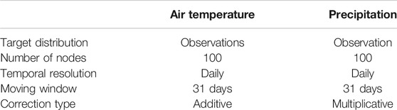
TABLE 1. Quantile mapping of air temperature and precipitation.

TABLE 2

TABLE 2. Quantile mapping of relative humidity, solar radiation and wind speed for both conventional and asynchronous configurations of the hydroclimatic modeling chain.

Table 2 details how quantile mapping of HRW variables differs from the conventional to asynchronous modeling chains. To overcome the limited availability of HRW observations within the study area, the conventional configuration uses climate reanalyses as target distributions. Climate reanalyses are reconstruction of past climate through the blending of observations with numerical models that are spatially and temporally complete, they are thus produced from a consistent physical representation of the climate processes. On the other hand, reanalyses are known to be biased relative to observations in a magnitude that varies locally (Li et al., 2013; Jones et al., 2017; Martins et al., 2017). Recently, reanalyses have been used to provide target distributions for statistical post-processing of climate simulations (Grenier, 2018) and to force hydrologic models during calibration (Fuka et al., 2014; Lauri et al., 2014). Corresponding transfer functions are configured with 100 nodes and a monthly temporal resolution.

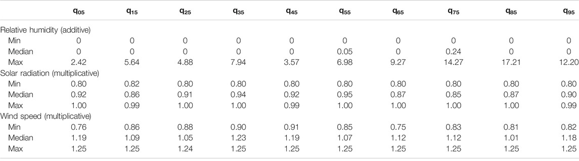
Table 2 also details how quantile mapping of HRW variables is applied within the asynchronous hydroclimatic modeling chain. Since transfer functions are calibrated minimizing the error affecting the simulated hydrologic response, no description of the observed climate system is required to define the target distributions. In order to set resolvable optimization problems, coarser transfer functions are defined (relative to the conventional configuration) using 10 nodes (instead of 100, from percentile 5 to percentile 95 by increments of 10) and an annual resolution (no subsampling of the annual cycle), instead of a monthly resolution. For both configurations, HRW variables are post-processed considering the 1980–2009 calibration period, without considering inter-variable relations (univariate quantile mapping) neither the application of a moving window is applied to post-processed variables. Correction is additive for relative humidity and multiplicative for solar radiation and wind speed.

Hydrologic Modeling

Hydrologic processes are simulated at a daily time step using WaSiM-ETH (Schulla, 2019), a distributed, physically based hydrologic model mostly operated for local and regional water resources assessments in Europe (Willkofer et al., 2018; Rössler et al., 2019) and more marginally in North America (Velázquez et al., 2013). An exhaustive description of the modeling setup is provided by Ricard and Anctil (2019). Snow accumulation and melt are simulated with a temperature-index degree-day approach while surface runoff is driven by precipitation intensity and hydraulic conductivity. Unsaturated vertical fluxes and transient soil hydraulic properties are based on Richards (Richards, 1931) and Van Genuchten equations (Van Genuchten, 1980). The portion of snow melt taken as surface runoff is defined empirically. Interflow simulation considers hydraulic conductivity and slope. Recession constants delay surface runoff and interflow. Reference evapotranspiration is assessed with the Penman-Montheith formulation (Allen et al., 1998).

Calibration

Both conventional and asynchronous configurations of the hydroclimatic modeling chain are calibrated with the PA-DDS multi-criteria optimization algorithm (Asadzadeh and Tolson, 2012). The calibration of the hydrologic model operates from 1980 to 1989 given an optimization budget of 500 iterations (the model is burned by running simulations from 1979). The calibration period of the hydrologic model is shorter relative to the quantile mapping calibration period in order to alleviate computational requirements of the optimization process. A 10-year period is generally considered sufficiently long for calibrating the hydrologic model. A bi-criteria asynchronous objective function (AOF, Ricard et al., 2019) is defined as:

$AOF=\left[RMS{D}_{Qa},RMS{D}_{Qn}\right],(2)$

where RMSD_Qa (Eq. 3) is the root mean square deviation between simulated (sim) and observed (obs) daily mean annual cycle for streamflow ($\overline{Q_{a,sim}}$ and $\overline{Q_{a,obs}}$) and RMSD_Qn (Eq. 4), between simulated and observed streamflow values below the 10th quantile (q₁₀) from June to November (JJASON).

$RMS{D}_{Qa}=\sqrt{\frac{{{\displaystyle \sum }}_{a=1}^{365}{\left(\overline{Q_{a,sim}}-\overline{Q_{a,obs}}\right)}^2}{365}},(3)$

$RMS{D}_{Qn}=\text{RMSD}{\left[Q_{sim}<Q_{sim}^{q_{10}},Q_{obs}<Q_{obs}^{q_{10}}\right]}_{JJASON},(4)$

The optimization algorithm assigns initial random values to the given transfer functions (TF) used to post-process climate variables as well as for the free parameters of the hydrologic model (h), defining a p-dimensions space such as:

$p_{v,t,q,h}=T{F}_{v,t,q}+h,(5)$

where v represents the post-processed climate variables, t and q stand for the temporal resolution and the number of nodes defining TF, respectively. Considering a given n-iterations optimization budget, the algorithm converges incrementally to an optimal parametric solution (P), which can be expressed as:

$P={p_{v,t,q,h}|}_n^{MIN\left(AOF\right)},(6)$

where MIN(AOF) stands for the minimization of a given asynchronous objective function (Ricard et al., 2019).

Tables 3Tables 4 present the calibration range of values assigned to HRW transfer functions and to hydrologic model free parameters. Boundaries of transfer functions are set according to a prequel evaluation of the bias of the climate simulation, piloting the optimization algorithm toward realistic values. According to (Eq. 5), the conventional configuration of the hydroclimatic modeling chain explores an 7-dimension space (v = 0 and p = 7), while the asynchronous configuration, a 37-dimension space (v = 3, q = 10 and p = 7). In order to assess equifinality (Beven and Freer, 2001) resulting from the asynchronous configuration, 16 realizations of the optimization process are conducted with independent random initial conditions (seeds). With the conventional configuration, 4 realizations are conducted for each (4) reanalysis, resulting also in 16 realizations of the optimization process.

TABLE 3

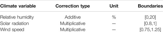
TABLE 3. Calibration range for relative humidity, solar radiation and wind speed transfer functions.

TABLE 4

TABLE 4. Calibration range of WaSiM-ETH free parameters.

Domain and Data

The study is conducted over the Du Loup catchment, Canada (515 km², Figure 2). The latter is characterized by moderate slopes (highest elevation is 600 m) and a dominant forested land use (77%). Monthly mean air temperature varies from −12°C to 18 °C and total precipitation reaches roughly 1,000 mm each year. Seasonal hydrologic fluctuations are driven by snow melt in spring and the intensification of synoptic liquid precipitation in autumn. Low flows are generally observed in winter and summer, due to the snow accumulation and the intensification of evapotranspiration, respectively.

FIGURE 2

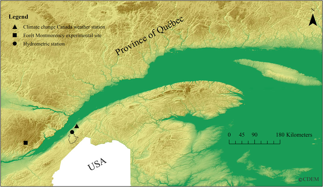
FIGURE 2. Du Loup catchment, Canada.

Table 5 describes the source of the climate data employed within the experimental design. Daily air temperature and precipitation are extracted from the gridded interpolated product provided by Livneh et al. (2015), from 1980 to 2009. They are used as target distributions applying conventional quantile mapping to simulated air temperature and precipitation and for forcing the hydrological model during calibration. Observed wind speed and relative humidity are taken from Environment and Climate change Canada weather monitoring network (station 7056616, 47.81°N and −69.55°E, 26 km north from Du Loup catchment, Figure 2), from 1994 to 2009. Downwelling shortwave radiation observations are collected at the Forêt Montmorency experimental site (Isabelle et al., 2018; 47.27°N and −71.12°E, Figure 2), from 2016 to 2018. The latter is located 120 km west from Du Loup catchment, with similar latitudes. It is important to clarify that HRW observations are exclusively given as reference in order to estimate biases of reanalyses and post-processed variables, consequently they are not employed for operating quantile mapping nor calibrating the hydrologic model.

TABLE 5

TABLE 5. Sources and usages of climate data.

HRW variables are also taken from four common reanalyses, namely the NCEP Climate Forecast System Reanalysis (CFSR, Saha et al., 2014), the NASA-Modern Era Retrospective-analysis for Research and Applications, Version 2 (MERRA-2, Gelaro et al., 2017), the European Center for Medium-Range Weather Forecasting (ECMWF) reanalysis (ERA-Interim, Dee et al., 2011), and the Japanese 55-years atmospheric reanalysis (JRA-55, Chen et al., 2014; Kobayashi et al., 2015). Relative humidity, solar radiation, and wind speed, taken from 1980 to 2009 and aggregated into a daily time step, are used as target distributions operating conventional quantile mapping. Simulated daily air temperature, precipitation, relative humidity, solar radiation, and wind speed are finally taken from three members of the CRCM5-LE (Canadian Regional Climate Model Large Ensemble, Leduc et al., 2019; von Trentini et al., 2019). CRCM5-LE follows RCP8.5 and is used for constructing streamflow simulations from 1955 to 2100.

Daily streamflow observations are taken from Quebec Hydrometric Network (station 022507, 47.61°N, −69.64°E, data available since 1978). A burned 50-m digital elevation model (DEM) and land use information are provided by Quebec Ministère de l’Environnement et de la Lutte contre les Changements Climatique (MELCC, 2016). Soil texture are assessed based the global soil data set collected by Shangguan et al. (2014). Physiographic data are aggregated to a 500-m resolution.

Results

Relative Humidity, Solar Radiation, and Wind Speed Variables From Reanalyses

Figure 3 presents daily mean annual cycles for HRW variables issued by MERRA-2, CFSR, ERA-Interim, and JRA-55 reanalyses for the Du Loup catchment between 1980 and 2009. Corresponding empirical cumulative distribution functions (ecdfs) constructed from daily values (mean in the case of relative humidity and wind speed, summed, in the case of solar radiation) are also presented. Available observations from nearby sites are also given as reference (black dotted lines). The observed daily mean annual cycle of relative humidity (Figure 3A) presents moderate seasonal fluctuations, ranging from 70% in winter and early spring to 80% in summer and autumn. All reanalyses fail in representing the seasonal fluctuations of the relative humidity. CFSR and JRA-55 provide notable overestimations in winter and spring (∼+20%). Most reanalyses underestimate relative humidity in summer and early autumn (∼−5%–10%), except for CFSR that issues a more accurate representation. Winter biases related to CFSR and JRA-55 cause systematic overestimations of the ecdfs (Figure 3D) while MERRA-2 and ERA-Interim are much closer to the observations.

FIGURE 3

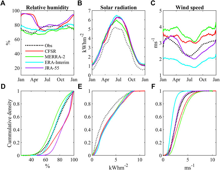
FIGURE 3. Relative humidity, solar radiation, and wind speed issued by CFRS, MERRA-2, ERA-Interim and JRA-55 reanalyses over Du Loup catchment between 1980 and 2009. First row presents daily mean annual cycles. Second row presents corresponding empirical cumulative distribution functions issued from daily values. Observations from neighboring meteorological stations (dashed black) and from Forêt Montmorency experimental site (dashed gray, 120 km) are given as a reference.

As expected, the daily mean annual cycle of solar radiation (Figure 3B) is characterized by a marked seasonal fluctuation, ranging from 0.5 kW h m⁻² in January up to 5.5 kW h m⁻² around the summer solstice. Solar radiation issued from one reanalysis to another is comparable except for MERRA-2 that provides lower values in spring and summer. Reanalyses systematically overestimate solar radiation relative to observation. The short length of the observation chronicle (2016–2018) and the distance from the studied site (120 km) must be taken into account as important limitations while assessing the biases affecting solar radiation issued from reanalyses. No closer observations exist.

The daily mean annual cycle of wind speed (Figure 3C) is lowest in summer (∼2.2 m s⁻¹) but fairly constant and higher otherwise (∼3 m s⁻¹). Reanalyses tend to provide a sound representation of the seasonal wind fluctuations. They differ, however, one from the other by the scale of annual biases. JRA-55 provides the most accurate representation of the wind speed annual cycle (confirmed by corresponding ecdf). CFSR and MERRA-2 moderately overestimate mean annual wind speed (∼+0.5 m s⁻¹ and ∼+1 m s⁻¹, respectively), while ERA-Interim underestimates wind speed values throughout the year (∼−1 m s⁻¹).

Post-processed Simulations of Relative Humidity, Solar Radiation, and Wind Speed Variables

Figures 4A–C illustrate daily mean annual cycles for HRW variables from the raw CRCM5-LE simulations (no statistical post-processing) for the Du Loup catchment between 1980 and 2009. The figure also illustrates corresponding post-processed HRW simulations issued by both conventional (Figure 4D–F) and asynchronous (Figure 4G–I) hydroclimatic chains. Available observations are given as a reference. Transfer function quantile values optimized by the asynchronous configuration are given in Appendix. Discrepancies between simulated HRW variables and corresponding observations may be explained by the distance of neighboring meteorological stations observations (120 km in the case of solar radiation), but also by other external factors such as vegetation or elevation.

FIGURE 4

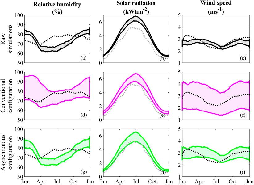
FIGURE 4. Daily mean annual cycles for relative humidity, solar radiation, and wind speed issued by CRMC5-LE over Du Loup catchment between 1980 and 2009. First row presents raw simulations (black, spread given by three CRCM5-LE members). Second and third rows present post-processed variables issued by conventional (magenta, three members and four reanalysis) and asynchronous (green, three members and 16 optimization realizations) configurations of the hydroclimatic modeling chain. Observations from neighboring meteorological stations (dashed black) and from Forêt Montmorency experimental site (dashed gray, 120 km) are given as reference.

As for reanalyses (Relative Humidity, Solar Radiation, and Wind Speed Variables From Reanalyses), CRCM5-LE raw simulations fail in representing seasonal fluctuations of relative humidity (Figure 4A), the latter is overestimated in winter and underestimated in summer. The spread of post-processed simulations issued by the conventional configuration increases notably in respect to the raw simulations (Figure 4D), these latter replicating biases embedded within the reanalyses employed as target distributions for the quantile mapping. Post-processed simulations tend to reduce summer biases relative to raw simulations but to overestimate relative humidity in winter. The asynchronous configuration issued equivalent seasonal fluctuations of relative humidity (Figure 4G) in comparison to raw simulations, reducing the spread of post-processed simulations in comparison to the conventional configuration.

Raw simulations of solar radiation (Figure 4B) are similar to reanalyses, these latter systematically overestimating available observations. Post-processed simulations issued by both configurations show comparable features (Figures 4E,H). The spread of post-processed simulations is generally higher relative to raw simulations; bias is also smaller.

Raw simulations of wind speed (Figure 4C) provide a sound representation of the annual cycle, bias is small and seasonal fluctuations accurately represented. As for the relative humidity, the spread of post-processed simulations issued by the conventional configuration (Figure 4F) is much larger relative to the raw simulations, these latter also replicating biased embedded within the reanalyses. An enlargement in the spread of post-process simulations issued by the asynchronous configuration is again observable (Figure 4I), but to a lesser extent.

Streamflow Simulations and Projections

Figure 5 illustrates an example of WaSiM-ETH simulated streamflow driven by CRCM5-LE climate simulations, over the reference period (1980–2009). Conventional and asynchronous configurations of the hydroclimatic modeling chain are compared to raw climate simulations. Optimized values of WaSiM-ETH free parameters are given in Appendix. One can observe that raw climate simulations and conventional configuration tend to generate spring flood too early (Figure 5A), while raw simulations underestimate its magnitude. On the other hand, the asynchronous configuration reproduces more accurately spring flood synchronicity and magnitude. All simulations tend to overestimate mean flow from August to October, which is more noticeable for the conventional configuration. Low flow overestimation is confirmed in Figure 5B for both the conventional configuration and raw simulations, whereas the asynchronous configuration offering a more accurate ecdf. Annual hydrographs (Figures 5C-K) confirm that all simulations depict the same sequence of hydrologic events. A higher variability in high flow values issued by the asynchronous configuration is also noticeable.

FIGURE 5

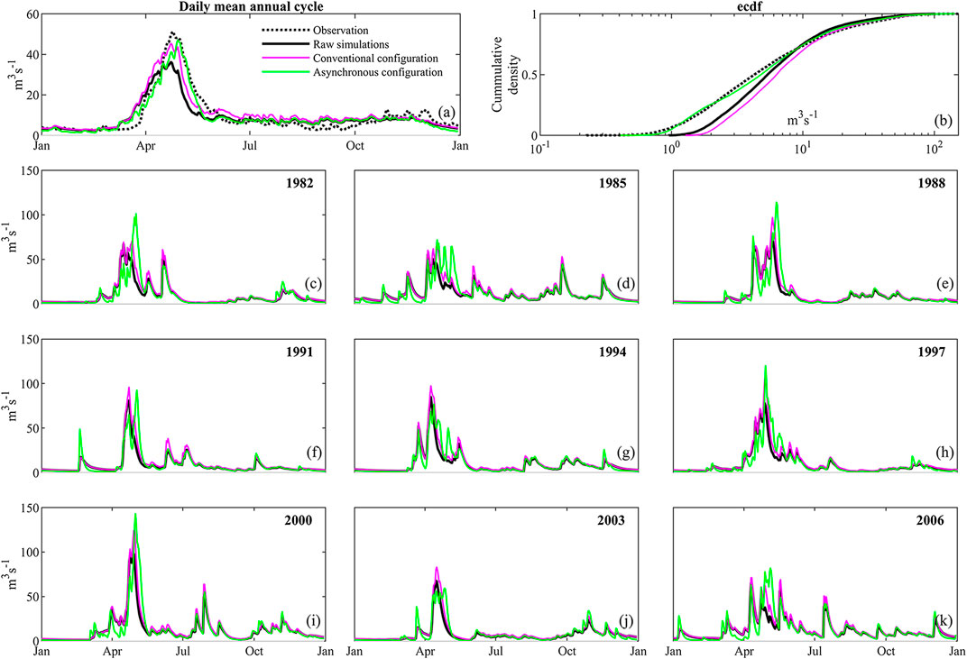
FIGURE 5. Streamflow simulations issued by CRCM5-LE climate simulations forcing the WaSiM-ETH hydrologic model over Du Loup catchment between 1980 and 2009. First row presents daily mean annual cycles and corresponding empirical cumulative distribution functions (ecdf) of daily values. Streamflow observations (dashed black) are given as reference. Following rows present a sample of simulated annual hydrographs (time step of 3 years, from 1980 to 2009). Streamflow simulations issued by conventional (magenta) and asynchronous (green) configurations of the hydroclimatic modeling chain are compared to raw climate simulations (full black).

Figure 6 compares the performance of streamflow simulations over the reference period. Performance is expressed through the root mean squared deviation (RMSD) applied to the annual cycle (Figure 6A), the inverse empirical cumulative distribution function (ecdf⁻¹, Figure 6B), and seasonal quantile values (Figures 6C-K). Each distribution is composed of 16 realizations of the optimization process. Considering median RMSD values, both conventional and asynchronous configurations provide an improved representation of the annual cycle and ecdf⁻¹ in comparison to the raw simulations. Asynchronous modeling offers, however, a much more accurate representation of seasonal extreme values (Figures 6C–E,I–K). As an example, from Figure 6E, the mean RMSD value computed on pluvial low flows is 0.37 m³ s⁻¹ for the asynchronous configuration, 1.09 m³ s⁻¹ for the conventional configuration, and 0.64 m³ s⁻¹ for raw simulations. Asynchronous modeling also offers a more robust representation of the hydrologic regime; RMSD values are systematically affected by a smaller spread. Conventional modeling provides a comparable (sometime weaker) representation of seasonal extreme values relative to raw climate simulations. It is also more prone to provide outlying degraded performance.

FIGURE 6

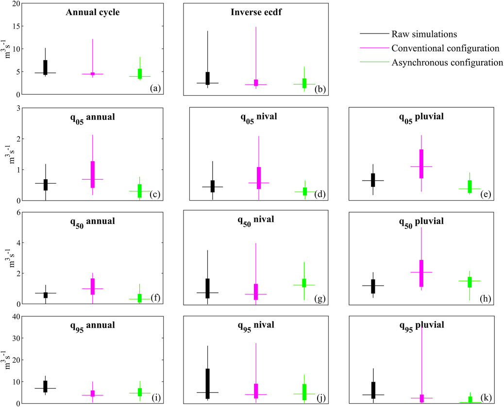
FIGURE 6. Performance of streamflow simulations issued by raw climate simulations (black), conventional (magenta) and asynchronous (green) configurations model over Du Loup catchment from 1980 to 2009. Performance is expressed through the root mean square deviation (RMSD). First line presents the daily mean annual cycle and the inverse empirical cumulative distribution function (ecdf⁻¹). Following lines present seasonal quantiles values (q₀₅, q₅₀, and q₉₅). The nival season runs from December to May, the pluvial season, from June to November. Each distribution is composed by 16 realizations of the optimization process.

Figure 7 illustrates the projected change of eight hydrologic indicators (Table 6) from 1980–2009 to 2040–2069 using raw simulation, conventional and asynchronous hydroclimatic modeling chain. For each indicator, 48 change values are evaluated: 3 climate simulation realizations (members) and 16 optimization realizations (seeds). Projections are first expressed through the magnitude of change, which is assessed using the median of the 48 projected changes. All runs project an increase in mean flow (+4.5% to +5.5%), nival high flow (+6.3% to +9.2%), and evapotranspiration (+13% to +16%). They also project a decrease in pluvial high flow (−3% to −9%) and snow water equivalent (−3% to −7%). They also agree on the direction of change affecting low flows, even if the magnitudes of the projected change are noticeably different.

FIGURE 7

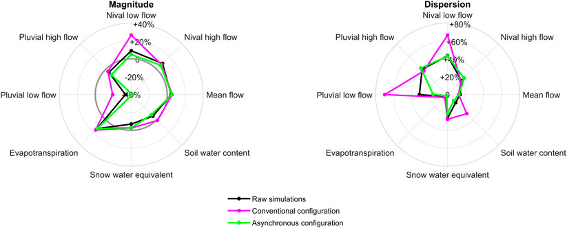
FIGURE 7. Projected change of hydrologic indicators over Du Loup catchment from 1980–2009 to 2040–2069. Changes issued by the conventional (magenta) and asynchronous (green) configurations of the hydroclimatic modeling chain are compared to raw climate simulations (black). Each distribution is composed by 48 change values (16 realizations of the optimization process × 3 climate simulation members) expressed as percentage. The magnitude of change corresponds to the median change value, while the dispersion, to the absolute difference between 10th and 90th percentiles.

TABLE 6

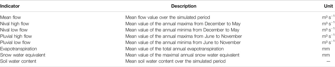
TABLE 6. Description of hydrologic indicators.

Conventional modeling projects a much higher increase in nival low flow (+26%) relative to raw simulations (+9%) and asynchronous modeling (+5%). Conventional modeling also projects a much smaller decrease in pluvial low flow (−19%) relative to raw simulations (−34%) and asynchronous modeling (−41%). Finally, projections disagree on soil water content. Conventional modeling projects a small increase (+1%), while raw simulations (−6%) and asynchronous modeling (−8%), a decrease. Figure 7 also presents the dispersion of change, namely the spread affecting the projected change values expressed by the 10th and 90th percentile interval (absolute difference). Conventional modeling provides more scattered projections for low flows (both nival and pluvial), and soil water content relative to raw simulations and asynchronous modeling. The spread affecting other hydrologic indicator does not appear much affected by the configuration of the hydroclimatic modeling chain.

Discussion

Relative humidity, solar radiation, and wind speed (HRW variables) have been introduced into a full hydroclimatic modeling chain using an asynchronous configuration adapted from Ricard et al. (2019), allowing the construction of streamflow projections using the Penman-Montheith reference evapotranspiration formulation. The WaSiM-ETH hydrologic model was driven with post-processed climate variables while quantile mapping transfer functions were calibrated together with the parameters of the hydrologic model, minimizing the asynchronous error affecting the simulated hydrologic response. The suggested approach circumvents the requirement for reference HRW observations, the latter placing an important limitation in representing energy-driven hydrological processes in many countries such as Canada.

Asynchronous hydroclimatic modeling provided a fairly accurate representation of post-processed solar radiation and wind speed in comparison to conventional quantile mapping using reanalyses as target distributions. Figures 3Figures 4 clearly depicted how conventional quantile mapping mimics biases affecting HRW variables issued by CFSR, MERRA-2, ERA-Interim, and JRA-55 reanalyses. Asynchronous hydroclimatic modeling did not, however, overcome major mismatches in seasonal fluctuations affecting raw simulations of relative humidity. Post-processed variables issued from the asynchronous configuration are fairly similar to raw simulations, suggesting the simulated hydrologic response is sensitive to the consistency between post-processed variables. Increasing transfer-function temporal resolution or broadening the range of values assigned for calibration could improve the accuracy of post-processed relative humidity issued by the asynchronous configuration, most likely to the expense of the consistency between post-processed variables. Since optimized transfer functions are constrained in providing the best available hydrologic performance, they guaranty sound driving conditions from the perspective of the hydrologic model.

The suggested asynchronous configuration to the hydroclimatic modeling chain assumes the hydrologic regime of a given catchment as a functional proxy to corresponding climate drivers. In other words, and in the case of this study, it circumvents the requirement for meteorological observations by exploiting streamflow observations as a surrogate to reference HRW observations. Comparable hypotheses have been proposed in paleoclimatology and paleohydrology (Lamarche, 1978; Case and MacDonald, 2003), but not (at least to our knowledge) for modeling the impact of climate change on water resources. Instead of integrating scarce HRW observations (or biased representation issued from reanalyses) into the modeling chain, these latter have been used to pilot the calibration process toward realistic solutions.

Results illustrated in Figures 5Figures 6 confirm that the asynchronous modeling issued a better representation of the hydrologic regime (annual cycle and empirical distributions) relative to conventional modeling and a much more accurate representation of extreme seasonal events (high and low flows, nival and pluvial seasons). Conventional modeling presented notable flaws in representing seasonal extreme values, corresponding performances being sometime weaker in comparison to raw climate simulations. It also appeared more vulnerable in producing outlying degraded performances. This can be explicated by the limited capacity of the hydrologic model to compensate for biased embedded within forcing post-processed HRW variables. Consequently, an evaluation of reanalyses biases appears highly recommendable as a prerequisite to the implementation of the conventional configuration, keeping in mind that reanalysis products are constantly updated and potentially improved. Since asynchronous hydroclimatic modeling assumes streamflow fluctuations as functional proxies to climate drivers, the hydrologic model was implemented aiming to limit parametric compensation as much as possible. No empirical correction was applied to simulated evapotranspiration and a fairly limited number of free parameters were available for calibration. The usage of empirical correction factors for evapotranspiration or additional free parameters would probably improve the simulated hydrologic response issued by conventional modeling, but possibly to the expense of injecting parametric instability into streamflow projections (Brigode et al., 2013).

Since the projected changes of the hydrologic regime varies from one configuration to another, one can argue that the scarcity of HRW observations contributes to uncertainty affecting physically based streamflow projections. By construction, the suggested asynchronous configuration the hydroclimatic modeling chain alters the nature of this uncertainty, trading-off a biased representation of the HRW variables issued from reanalyses with equifinality (Beven and Freer, 2001). Equifinality is directly related to the definition of the optimization problem and will generally increase with additional degrees of freedom (free parameters) to explore. In the context of the study, Eq. 5 clarifies how calibrating HRW transfer functions increases the scale of the parametric space in relation to post-processed variables, as for the number of nodes and the temporal resolution defining calibrated transfer functions. Figures 6Figures 7 confirmed that uncertainty affecting simulated streamflow projections is less impacted implementing the asynchronous configuration relative to integrating biased HRW variables into the conventional configuration, thus affecting post-processed variables and calibrated parameters of the hydrologic model. Asynchronous modeling appears more capable in producing a balanced trade-off between an accurate simulated hydrologic response over the reference period and a diminished uncertainty affecting the projection of hydrologic indicators. We thus conclude that asynchronous modeling contributes in increasing the confidence attributed to streamflow projections, this being even more noticeable for low flows and soil water content.

This study explored an alternative methodological framework aiming to integrate HRW variables to hydroclimatic modeling on a domain such as Canada where observations are too scarce to implement a conventional configuration of the modeling chain. As a demonstration, the suggested approach allowed the construction of streamflow projections using the Penman-Montheith physically based reference evapotranspiration formulation. We believe this innovative framework offers promising perspectives in the scope of consolidating the physical representation of hydrologic processes at the catchment scale and consequently, the confidence attributed to climate change impact analyses on water resources. We argue that by calibrating the whole modeling chain simultaneously, the accurate streamflow measurements allow to reconstruct the meteorological drivers, if enough care is taken not to overparameterize the optimization problem and to keep the parameters within physically reasonable ranges. We invite our fellow scientists to further explore the applicability of the suggested framework integrating additional water-related, energy-driven processes such as snow accumulation and melt, river ice jams, water temperature, or vegetal growth, confirming (or not) the added value of physically based representations relative to empirical formulations within non-stationary climate conditions. We finally acknowledge significant limitations of the experimental design and most importantly, the use of a single climate model. Generalizing asynchronous modeling to larger climate simulation ensembles (such as CMIP5) will require optimization strategy adapted to potentially very large parametric space to explore, suggesting constrains in terms of computational capacities and equifinality. Since quantile mapping is known to be prone to overfitting (Lafon et al., 2013), the sensitivity of streamflow projections to the selection of a given calibration period should also be addressed. Further works should also aim to construct the asynchronous configuration to precipitation and temperature, to larger (regional) domain using multi-site calibration techniques (Choi et al., 2015; Gaborit et al., 2015; Xue et al., 2016), and to preserve inter-variable correlations between post-processed fields (Dekens et al., 2017; Canon, 2018). Experimenting asynchronous modeling on highly monitored catchments would provide a more robust validation of post-processed climate simulations and also clarify the role of parametric compensation on the resulting uncertainty affecting streamflow projections.

Conclusion

The construction of streamflow projections generally involves a hydroclimatic modeling chain including statistical post processing of climate simulations and calibration of a hydrologic model. Since sufficiently long and dense chronicles are mandatory for the implementation of conventional configurations of the hydroclimatic chain, the scarcity of relative humidity, solar radiation, and wind speed (HRW) observations places an important limitation to the construction of physically based streamflow projections. The current study designed and explored an asynchronous configuration to the hydroclimatic modeling chain that circumvents the requirement for meteorological observations while operating quantile mapping and calibration of the hydrologic model. Asynchronous hydroclimatic modeling assumes streamflow fluctuations are functional proxies to corresponding climate drivers and is implemented by 1) driving the hydrologic model with post-processed climate simulations instead of meteorological observations and 2) calibrating quantile mapping transfer functions together with the parameter of the hydrologic model, minimizing the asynchronous error affecting the simulated hydrologic response over the reference period simulated by the forcing climate model.

Implementing this innovative framework, relative humidity, solar radiation, and wind speed variables have been introduced into a full hydroclimatic modeling chain, thus permitting the construction of streamflow projections using the Penman-Montheith physically based reference evapotranspiration. Except for relative humidity, results demonstrated a fairly accurate representation of post-processed variables relative to conventional quantile mapping using reanalyses as description of the climate system, ensuring a sound representation of climate drivers “from the perspective of the hydrologic model.” Results also demonstrated a more accurate and robust simulated hydrologic response issued from asynchronous modeling, suggesting an increased confidence attributed to resulting streamflow projections. The projection of low flows and soil water contents were sensitive to the configuration of the hydroclimatic modeling chain, confirming the scarcity of HRW observations as a notable contributor to uncertainty affecting physically based streamflow projections. We believe the suggested methodological framework opens promising perspectives in the scope of producing more reliable streamflow projections, but also estimations of water-related and energy-driven processes such as snow accumulation and melt, river ice jams, water temperature, or vegetation growth under evolving climate conditions.

Data Availability Statement

The raw data supporting the conclusions of this article will be made available by the authors, without undue reservation.

Author Contribution

SR and FA designed the experiments and SR carried them out. SR developed the model code and performed the simulations. SR prepared the manuscript with contributions from all co-authors.

Funding

This research was funded by the Mitacs Accelerate program for scholarship to SR (IT12297) with the contributions of Ouranos and the Québec Ministry of Forests, Wildlife and Parks (MFFP project #142332118).

Conflict of Interest

The authors declare that the research was conducted in the absence of any commercial or financial relationships that could be construed as a potential conflict of interest.

Acknowledgments

The production of ClimEx was funded within the ClimEx project by the Bavarian State Ministry for the Environment and Consumer Protection. The CRCM5 was developed by the ESCER center of Université du Québec à Montréal (UQAM; www.escer.uqam.ca) in collaboration with Environment and Climate change Canada. We acknowledge Environment and Climate change Canada’s Canadian Center for Climate Modeling and Analysis for executing and making available the CanESM2 Large Ensemble simulations used in this study, and the Canadian Sea Ice and Snow Evolution Network for proposing the simulations. Computations with the CRCM5 for the ClimEx project were made on the SuperMUC supercomputer at Leibniz Supercomputing Center (LRZ) of the Bavarian Academy of Sciences and Humanities. The operation of this supercomputer is funded via the Gauss Center for Supercomputing (GCS) by the German Federal Ministry of Education and Research and the Bavarian State Ministry of Education, Science and the Arts. Authors also wish to acknowledge Quebec Ministry of Environment and Fight Against Climate Change (MELCC) for interpolated meteorological data (precipitation and temperature), hydrometric data, digital representation of the river network and integrated description of land uses. Humidity and wind data were provided by Environment and Climate Canada. A special credit to Patrick Grenier (Ouranos) for challenging and structuring the proposed methodological framework.

Appendix

TABLE A1

TABLEA2

References

Allen, R. G., Pereira, L. S., Raes, D., and Smith, S. (1998). Crop evapotranspiration-guidelines for computing crop water requirements, Irrigation and drainage paper 56. Rome, Italy:FAO, 15.

Google Scholar

Arheimer, B., and Lindström, G. (2015). Climate impact on floods: changes in high flows in Sweden in the past and the future (1911-2100). Hydrol. Earth Syst. Sci. 19, 771–784, doi:10.5194/hess-19-771-2015 CrossRef Full Text

Google Scholar

Asadzadeh, M., and Tolson, B. (2012). Hybrid Pareto archived dynamically dimensioned search for multi-objective combinatorial optimization: application to water distribution network design. J. Hydroinf. 14, 192–205. doi:10.2166/hydro.2011.098 CrossRef Full Text

Google Scholar

Beven, K., and Freer, J. (2001). Equifinality, data assimilation, and uncertainty estimation in mechanistic modelling of complex environmental systems using the GLUE methodology. J. Hydrol. 249, 11–29. doi:10.1016/s0022-1694(01)00421-8 CrossRef Full Text

Google Scholar

Boulard, D., Castel, T., Camberlin, P., Sergent, A.-S., Bréda, N., Badeau, V., et al. (2016). Capability of a regional climate model to simulate climate variables requested for water balance computation: a case study over northeastern France. Clim. Dynam. 46, 2689–2716. doi:10.1007/s00382-015-2724-9 CrossRef Full Text

Google Scholar

Brigode, P., Oudin, L., and Perrin, C. (2013). Hydrological model parameter instability: a source of additional uncertainty in estimating the hydrological impacts of climate change? J. Hydrol. 476, 410–425. doi:10.1016/j.jhydrol.2012.11.012 CrossRef Full Text

Google Scholar

Cannon, A. J. (2018). Multivariate quantile mapping bias correction: an N-dimensional probability density function transform for climate model simulations of multiple variables. Clim. Dyn. 50, 31–49, doi:10.1007/s00382-017-3580-6 CrossRef Full Text

Google Scholar

Case, R. A., and MacDonald, G. M. (2003). Tree ring reconstructions of streamflow for three Canadian prairie Rivers. J. Am. Water Resour. Assoc. 39, 703–716. doi:10.1111/j.1752-1688.2003.tb03686.x CrossRef Full Text

Google Scholar

Chen, G., Iwasaki, T., Qin, H., and Sha, W. (2014). Evaluation of the warm-season diurnal variability over east asia in recent reanalyses JRA-55, ERA-interim, NCEP CFSR, and NASA MERRA. J. Clim. 27, 5517–5537. doi:10.1175/JCLI-D-14-00005.1 CrossRef Full Text

Google Scholar

Choi, Y. S., Choi, C. K., Kim, H. S., Kim, K. T., and Kim, S. (2015). Multi-site calibration using a grid-based event rainfall-runoff model: a case study of the upstream areas of the Nakdong River basin in Korea. Hydrol. Process. 29, 2089–2099. doi:10.1002/hyp.10355 CrossRef Full Text

Google Scholar

Dams, J., Nossent, J., Senbeta, T. B., Willems, P., and Batelaan, O. (2015). Multi-model approach to assess the impact of climate change on runoff. J. Hydrol. 529, 1601–1616. doi:10.1016/j.jhydrol.2015.08.023 CrossRef Full Text

Google Scholar

Das, T., Maurer, E. P., Pierce, D. W., Dettinger, M. D., and Cayan, D. R. (2013). Increases in flood magnitudes in California under warming climates. J. Hydrol. 501, 101–110. doi:10.1016/j.jhydrol.2013.07.042 CrossRef Full Text

Google Scholar

Dee, D. P., Uppala, S. M., Simmons, A. J., Berrisford, P., Berrisford, P., Poli, P., Kobayashi, S., et al. (2011). The ERA-interim reanalysis: configuration and performance of the data assimilation system. Q. J. R. Meteorol. Soc. 137, 553–597. doi:10.1002/qj.828 CrossRef Full Text

Google Scholar

Dekens, L., Parey, S., Grandjacques, M., and Dacunha-Castelle, D. (2017). Multivariate distribution correction of climate model outputs: a generalization of quantile mapping approaches. Environmetrics 28, e2454. doi:10.1002/env.2454 CrossRef Full Text

Google Scholar

Didovets, I., Krysanova, V., Bürger, G., Snizhko, S., Balabukh, V., and Bronstert, A. (2019). Climate change impact on regional floods in the Carpathian region. J. Hydrol. Reg. Stud. 22, 100590. doi:10.1016/j.ejrh.2019.01.002 CrossRef Full Text

Google Scholar

Feng, S., Trnka, M., Hayes, M., and Zhang, Y. (2017). Why do different drought indices show distinct future drought risk outcomes in the U.S. Great Plains? J. Clim. 30, 265–278. doi:10.1175/JCLI-D-15-0590.1 CrossRef Full Text

Google Scholar

Fuka, D. R., Walter, M. T., MacAlister, C., Degaetano, A. T., Steenhuis, T. S., and Easton, Z. M. (2014). Using the climate forecast system reanalysis as weather input data for watershed models. Hydrol. Process. 28, 5613–5623. doi:10.1002/hyp.10073 CrossRef Full Text

Google Scholar

Gaborit, É., Ricard, S., Lachance-Cloutier, S., Anctil, F., and Turcotte, R. (2015). Comparing global and local calibration schemes from a differential split-sample test perspective. Can. J. Earth Sci. 52, 990–999. doi:10.1139/cjes-2015-0015 CrossRef Full Text

Google Scholar

Gelaro, R., McCarty, W., Suárez, M. J., Todling, R., Molod, A., Takacs, L., et al. (2017). The modern-Era Retrospective analysis for research and applications, version 2 (MERRA-2), J. Clim. 30, 5419–5454. doi:10.1175/JCLI-D-16-0758.1 CrossRef Full Text

Google Scholar

Grenier, P. (2018). Two types of physical inconsistency to avoid with univariate quantile mapping: a case study over North America concerning relative humidity and its parent variables. J. Appl. Meteor. Climatol. 57, 347–364. doi:10.1175/JAMC-D-17-0177.1 CrossRef Full Text

Google Scholar

Isabelle, P.-E., Nadeau, D. F., Asselin, M.-H., Harvey, R., Musselman, K. N., Rousseau, A. N., et al. (2018). Solar radiation transmittance of a boreal balsam fir canopy: spatiotemporal variability and impacts on growing season hydrology. Agric. For. Meteorol. 263, 1–14. doi:10.1016/j.agrformet.2018.07.022 CrossRef Full Text

Google Scholar

Jones, P. D., Harpham, C., Troccoli, A., Gschwind, B., Ranchin, T., Wald, L., et al. (2017). Using ERA-interim reanalysis for creating datasets of energy-relevant climate variables. Earth Syst. Sci. Data. 9, 471–495. doi:10.5194/essd-9-471-2017 CrossRef Full Text

Google Scholar

Kay, A. L., Bell, V. A., Blyth, E. M., Crooks, S. M., Davies, H. N., and Reynard, N. S. (2013). A hydrological perspective on evaporation: historical trends and future projections in Britain. J. Water Clim. Chang. 4, 193–208. doi:10.2166/wcc.2013.014 CrossRef Full Text

Google Scholar

Kobayashi, S., Ota, Y., Harada, Y., Ebita, A., Moriya, M., Onoda, H., et al. (2015). The JRA-55 reanalysis: general specifications and basic characteristics. J. Meteorol. Soc. Jpn. 93, 5–48. doi:10.2151/jmsj.2015-001 CrossRef Full Text

Google Scholar

Lafon, T., Dadson, S., Buys, G., and Prudhomme, C. (2013). Bias correction of daily precipitation simulated by a regional climate model: a comparison of methods. Int. J. Climatol. 33, 1367–1381. doi:10.1002/joc.3518 CrossRef Full Text

Google Scholar

Lamarche, V. C. (1978). Tree-ring evidence of past climatic variability. Nature 276, 334–338. doi:10.1038/276334a0

CrossRef Full Text | Google Scholar

Lauri, H., Räsänen, T. A., and Kummu, M. (2014). Using reanalysis and remotely sensed temperature and precipitation data for hydrological modeling in monsoon climate: mekong river case study. J. Hydrometeorol. 15, 1532–1545. doi:10.1175/JHM-D-13-084.1 CrossRef Full Text

Google Scholar

Leduc, M., Mailhot, A., Frigon, A., Martel, J.-L., Ludwig, R., Brietzke, G. B., et al. (2019). The ClimEx project: a 50-member ensemble of climate change projections at 12-km resolution over Europe and northeastern north America with the Canadian regional climate model (CRCM5). J. Appl. Meteor. Climatol. 58, 663–693. doi:10.1175/jamc-d-18-0021.1 CrossRef Full Text

Google Scholar

Li, J.-L. F., Waliser, D. E., Stephens, G., Lee, S., L'Ecuyer, T., Kato, S., et al. (2013). Characterizing and understanding radiation budget biases in CMIP3/CMIP5 GCMs, contemporary GCM, and reanalysis. J. Geophys. Res. Atmos. 118, 8166–8184. doi:10.1002/jgrd.50378 CrossRef Full Text

Google Scholar

Livneh, B., Bohn, T. J., Pierce, D. W., Munoz-Arriola, F., Nijssen, B., Vose, R., et al. (2015). A spatially comprehensive, hydrometeorological data set for Mexico, the U.S., and Southern Canada 1950–2013. Sci. Data. 2, 150042. doi:10.1038/sdata.2015.42

CrossRef Full Text | Google Scholar

Lofgren, B. M., Gronewold, A. D., Acciaioli, A., Cherry, J., Steiner, A., and Watkins, D. (2013). Methodological approaches to projecting the hydrologic impacts of climate change*. Earth Interact. 17, 1–19. doi:10.1175/2013EI000532.1 CrossRef Full Text

Google Scholar

Maraun, D., Shepherd, T. G., Widmann, M., Zappa, G., Walton, D., Gutiérrez, J. M., et al. (2017). Towards process-informed bias correction of climate change simulations. Nat. Clim. Change. 7, 764–773. doi:10.1038/NCLIMATE3418 CrossRef Full Text

Google Scholar

Martins, D. S., Paredes, P., Raziei, T., Pires, C., Cadima, J., and Pereira, L. S. (2017). Assessing reference evapotranspiration estimation from reanalysis weather products. An application to the Iberian Peninsula. Int. J. Climatol. 37, 2378–2397. doi:10.1002/joc.4852 CrossRef Full Text

Google Scholar

MELCC (2016). Utilisation du territoire. Méthodologie et description de la couche d’information géographique. Version 1.4. Québec City, Canada, 24

Google Scholar

Muerth, M. J., Gauvin St-Denis, B., Ricard, S., Velázquez, J. A., Schmid, J., Minville, M., Caya, D., et al. (2013). On the need for bias correction in regional climate scenarios to assess climate change impacts on river runoff. Hydrol. Earth Syst. Sci. 17, 1189–1204, doi:10.5194/hess-17-1189-2013 CrossRef Full Text

Google Scholar

Najafi, M. R., Moradkhani, H., and Jung, I. W. (2011). Assessing the uncertainties of hydrologic model selection in climate change impact studies. Hydrol. Process. 25, 2814–2826, doi:10.1002/hyp.8043 CrossRef Full Text

Google Scholar

Ott, I., Duethmann, D., Liebert, J., Berg, P., Feldmann, H., Ihringer, J., et al. (2013). High-resolution climate change impact analysis on medium-sized river catchments in Germany: an ensemble assessment. J. Hydrometeorol. 14, 1175–1193. doi:10.1175/JHM-D-12-091.1 CrossRef Full Text

Google Scholar

Rössler, O., Kotlarski, S., Fischer, A. M., Keller, D., Liniger, M., and Weingartner, R. (2019). Evaluating the added value of the new swiss climate scenarios for hydrology: an example from the Thur catchment. Clim. Ser. 13, 1–13. doi:10.1016/j.cliser.2019.01.001 CrossRef Full Text

Google Scholar

Reiter, P., Gutjahr, O., Schefczyk, L., Heinemann, G., and Casper, M. (2018). Does applying quantile mapping to subsamples improve the bias correction of daily precipitation? Int. J. Climatol. 38, 1623–1633. doi:10.1002/joc.5283 CrossRef Full Text

Google Scholar

Ricard, S., and Anctil, F. (2019). Forcing the penman-montheith formulation with humidity, radiation, and wind speed taken from reanalyses, for hydrologic modeling. Water 11, 1214–1215. doi:10.3390/w11061214 CrossRef Full Text

Google Scholar

Ricard, S., Sylvain, J.-D., and Anctil, F. (2019). Exploring an alternative configuration of the hydroclimatic modeling chain, based on the notion of asynchronous objective functions. Water 11, 2012–2018. doi:10.3390/w11102012 CrossRef Full Text

Google Scholar

Richards, L. A. (1931). Capillary conduction of liquids through porous mediums. Physics 1, 318–333. doi:10.1063/1.1745010 CrossRef Full Text

Google Scholar

Roy, T., Valdés, J. B., Lyon, B., Demaria, E. M. C., Serrat-Capdevila, A., Gupta, H. V., et al. (2018). Assessing hydrological impacts of short-term climate change in the Mara River basin of East Africa. J. Hydrol. 566, 818–829. doi:10.1016/j.jhydrol.2018.08.051 CrossRef Full Text

Google Scholar

Saha, S., Moorthi, S., Wu, X., Wang, J., Nadiga, S., Tripp, P., et al. (2014). The NCEP climate Forecast system version 2. J. Clim. 27, 2185–2208. doi:10.1175/JCLI-D-12-00823.1 CrossRef Full Text

Google Scholar

Schulla, J. (2019). Model description WaSiM. Available at: www.wasim.ch (accessed February 27, 2020).

Google Scholar

Seiller, G., and Anctil, F. (2016). How do potential evapotranspiration formulas influence hydrological projections? Hydrol. Sci. J. 61, 2249–2266. doi:10.1080/02626667.2015.1100302 CrossRef Full Text

Google Scholar

Shangguan, W., Dai, Y., Duan, Q., Liu, B., and Yuan, H. (2014). A global soil data set for earth system modeling. J. Adv. Model. Earth Syst. 6, 249–263. doi:10.1002/2013MS000293 CrossRef Full Text

Google Scholar

Shaw, S. B., and Riha, S. J. (2011). Assessing temperature-based PET equations under a changing climate in temperate, deciduous forests. Hydrol. Process. 25, 1466–1478. doi:10.1002/hyp.7913 CrossRef Full Text

Google Scholar

Smitha, P. S., Narasimhan, B., Sudheer, K. P., and Annamalai, H. (2018). An improved bias correction method of daily rainfall data using a sliding window technique for climate change impact assessment. J. Hydrol. 556, 100–118. doi:10.1016/j.jhydrol.2017.11.010 CrossRef Full Text

Google Scholar

Teutschbein, C., Grabs, T., Karlsen, R. H., Laudon, H., and Bishop, K. (2015). Hydrological response to changing climate conditions: spatial streamflow variability in the boreal region. Water Resour. Res. 51, 9425–9446. doi:10.1002/2015WR017337 CrossRef Full Text

Google Scholar

Themeßl, M. J., Gobiet, A., and Leuprecht, A. (2011). Empirical-statistical downscaling and error correction of daily precipitation from regional climate models. Int. J. Climatol. 31, 1530–1544. doi:10.1002/joc.2168

CrossRef Full Text | Google Scholar

Tramblay, Y., Amoussou, E., Dorigo, W., and Mahé, G. (2014). Flood risk under future climate in data sparse regions: linking extreme value models and flood generating processes, J. Hydrol. 519, 549–558. doi:10.1016/j.jhydrol.2014.07.052 CrossRef Full Text

Google Scholar

Van Genuchten, M. T. (1980). A closed-form equation for predicting the hydraulic conductivity of unsaturated soils. Soil Sci. Soc. Am. J. 44, 892–898. doi:10.2136/sssaj1980.03615995004400050002x

CrossRef Full Text | Google Scholar

Velázquez, J. A., Schmid, J., Ricard, S., Muerth, M. J., Gauvin St-Denis, B., Minville, M., et al. (2013). An ensemble approach to assess hydrological models' contribution to uncertainties in the analysis of climate change impact on water resources. Hydrol. Earth Syst. Sci. 17, 565–578, doi:10.5194/hess-17-565-2013 CrossRef Full Text

Google Scholar

von Trentini, F., Leduc, M., and Ludwig, R. (2019). Assessing natural variability in RCM signals: comparison of a multi model EURO-CORDEX ensemble with a 50-member single model large ensemble. Clim. Dynam. 50, 1963–1979. doi:10.1007/s00382-019-04755-8 CrossRef Full Text

Google Scholar

Willkofer, F., Schmid, F.-J., Komischke, H., Korck, J., Braun, M., and Ludwig, R. (2018). The impact of bias correcting regional climate model results on hydrological indicators for Bavarian catchments. J. Hydrol.: Reg. Stud. 19, 25–41. doi:10.1016/j.ejrh.2018.06.010 CrossRef Full Text

Google Scholar

Xue, X., Zhang, K., Hong, Y., Gourley, J. J., Kellogg, W., McPherson, R. A., et al. (2016). New multisite cascading calibration approach for hydrological models: case study in the red river basin using the VIC model. J. Hydrol. Eng. 21, 05015019. doi:10.1061/(ASCE)HE.1943-5584.0001282 CrossRef Full Text

Google Scholar