 Taylor Smith*Bodo Bookhagen
- Institute of Geosciences, Universität Potsdam, Potsdam, Germany
High Mountain Asia (HMA) is dependent upon both the amount and timing of snow and glacier meltwater. Previous model studies and coarse resolution (0.25° × 0.25°, ∼25 km × 25 km) passive microwave assessments of trends in the volume and timing of snowfall, snowmelt, and glacier melt in HMA have identified key spatial and seasonal heterogeneities in the response of snow to changes in regional climate. Here we use recently developed, continuous, internally consistent, and high-resolution passive microwave data (3.125 km × 3.125 km, 1987–2016) from the special sensor microwave imager instrument family to refine and extend previous estimates of changes in the snow regime of HMA. We find an overall decline in snow volume across HMA; however, there exist spatially contiguous regions of increasing snow volume—particularly during the winter season in the Pamir, Karakoram, Hindu Kush, and Kunlun Shan. Detailed analysis of changes in snow-volume trends through time reveal a large step change from negative trends during the period 1987–1997, to much more positive trends across large regions of HMA during the periods 1997–2007 and 2007–2016. We also find that changes in high percentile monthly snow-water volume exhibit steeper trends than changes in low percentile snow-water volume, which suggests a reduction in the frequency of high snow-water volumes in much of HMA. Regions with positive snow-water storage trends generally correspond to regions of positive glacier mass balances.
1. Introduction
Rivers draining from High Mountain Asia (HMA) are relied upon by more than a billion people for agriculture, hydropower, and household use (Immerzeel et al., 2010; Bolch et al., 2012; Vaughan et al., 2013). In much of HMA, snow and glacier meltwaters provide key seasonal water buffers that help maintain water availability year-round (Barnett et al., 2005; Bookhagen and Burbank, 2010; Immerzeel et al., 2010; Berghuijs et al., 2014; Lutz et al., 2014; Huss et al., 2017). A large body of research has identified significant changes in HMA’s cryosphere in recent decades, and in particular, the retreat of many regional glaciers (e.g., Hewitt, 2005; Déry and Brown, 2007; Scherler et al., 2011; Bolch et al., 2012; Gardelle et al., 2012; Kääb et al., 2012; Sorg et al., 2012; Kapnick et al., 2014; Wulf et al., 2016; Sakai and Fujita, 2017; Smith et al., 2017; Smith and Bookhagen, 2018; Lievens et al., 2019; Rounce et al., 2019; Treichler et al., 2019; Shean et al., 2020); however, there exist large spatial heterogeneities in glacier trends (Hewitt, 2005; Gardelle et al., 2012; Kääb et al., 2012; Yao et al., 2012; Sakai and Fujita, 2017; Treichler et al., 2019). Previous work has also identified spatial and seasonal patterns in snow depth and the timing of snowmelt in HMA, which are mostly coherent with changes in glacier mass balances (Smith et al., 2017; Smith and Bookhagen, 2018; Wang et al., 2018; Treichler et al., 2019; Notarnicola, 2020; Shean et al., 2020). In-depth analyses of changes in HMA’s cryosphere are often limited by lack of in-situ data and rugged terrain which hinders high-resolution data collection (Bookhagen and Burbank, 2010); estimates of climate trends from in-situ, satellite, and modeled data often result in heterogeneous and complex spatial patterns (Smith and Bookhagen, 2018).
Passive microwave data have long provided the best global dataset for studying snow depth and snow-water storage (Chang et al., 1982). However, they are limited by spatial resolution—data are typically available as 0.25° × 0.25° (∼25 km × 25 km) grid cells which hinders many analyses. Recently, the National Snow and Ice Data Center has re-gridded and re-processed the special sensor microwave imager (SSMI, 1987–2009) and special sensor microwave imager/sounder (SSMI/S, 2003–2016) to a 3.125 km × 3.125 km (∼10 km2) spatial resolution (Brodzik et al., 2016). In this study, we leverage this high-resolution, cross-calibrated, multi-satellite dataset to consider 1.02 million passive microwave grid cells over 29 complete October-September water years across HMA (25–45°N, 60–110°E, 1987–2016; Figure 1). The enhanced resolution of this dataset allows us to more closely examine spatio-temporal trends in snow-water storage which have previously been shown to have strong impacts on climate and glacier dynamics in the region (Zhao and Moore, 2004; Fujita and Nuimura, 2011; Kapnick et al., 2014; Smith and Bookhagen, 2018).
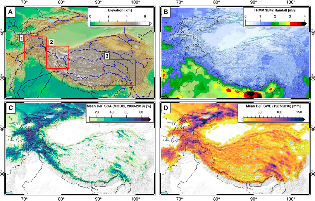
FIGURE 1. Study area (A) topography (B) average annual Tropical Rainfall Measurement Mission precipitation sum [0.25°, 1998–2018 (Huffman et al., 2007)], (C) average December-January-February (DJF) snow-covered area percentage from MODIS MOD10A [500 m, 2000–2019 (Hall and Riggs, 2016)], and (D) average DJF snow-water equivalent (SWE) volume from 3.125 km resolution special sensor microwave imager and special sensor microwave imager/sounder (1987–2016). Deep snow is generally confined to high-elevation regions. Blue outlines on (A) show major watersheds from HydroBASINS (Lehner and Grill, 2013), black lines show international borders. Labeled boxes indicate sub-areas shown in Figures 4 and 8.
2. Data and Methods
2.1. Study Area and Data Sources
Our study covers the region from 25 to 45°N and from 65 to 105°E, running across some of the most densely populated regions of the world. Several key watersheds, such as the Indus, Syr Darya, Amu Darya, Yangtze, Salween, and Ganges/Brahmaputra drain from HMA (Figure 1A, blue outlines).
Precipitation in HMA is driven by three main weather systems—the Indian Summer Monsoon, the East Asian Summer Monsoon, and the Winter Westerly Disturbances (Bookhagen and Burbank, 2010; Cannon et al., 2016b). These major weather systems interact to bring a heterogeneous mix of snow and rain to different regions of HMA. Recent changes in the timing and intensity of precipitation from these major weather systems have been observed (e.g., Kitoh et al., 2013; Menon et al., 2013; Vaughan et al., 2013; Cannon et al., 2015; Singh et al., 2014; Cannon et al., 2016b; Malik et al., 2016; Norris et al., 2020), and have been shown to impact the timing and volume of snow-water storage and snowmelt (Kapnick et al., 2014; Smith et al., 2017; Smith and Bookhagen, 2018).
2.2. Satellite Data Preparation
Snow has been extensively studied with passive microwave data—albeit at low spatial resolutions (e.g., 0.25° × 0.25°) (Chang et al., 1987; Kelly et al., 2003; Smith and Bookhagen, 2016; Smith and Bookhagen, 2018). Recent image processing advances have allowed researchers to take advantage of the elliptical nature of passive microwave footprints to re-process the data onto a much finer spatial grid than previous approaches had allowed. In this study, we use the EASE-grid 2.0 high-resolution passive microwave product (1987–2016) (Early and Long, 2001; Brodzik et al., 2012; Brodzik et al., 2016; Long and Brodzik, 2016), which provides the 19 and 37 GHz passive microwave frequencies at spatial resolutions of 6.25 and 3.125 km, respectively. This dataset has been carefully cross-calibrated between the various SSMI and SSMI/S satellite platforms to provide consistent and homogenized data through the entire time series (Brodzik et al., 2016).
To produce consistent snow-water equivalent (SWE) estimates over the entire study region, we further re-grid the 19 GHz passive microwave data to a 3.125 km spatial resolution. We then remove areas near lakes and areas with shallow or infrequent snow-cover, as these areas are not suitable for long-term SWE trend analysis. Finally, following the methodology of Smith and Bookhagen (2018), we use the computationally efficient algorithm proposed by Chang et al. (1987) to convert the passive microwave data to snow depth:
We then convert those snow depth estimates to SWE using a constant snow density of 0.24 g/cm3, which has been shown to be a reasonable global average (Sturm et al., 2010; Takala et al., 2011). In short, the Chang et al. (1987) algorithm uses the difference between the 19 and 37 GHz passive microwave channels to estimate snow depth based on a comparison with extensive snow survey data collected throughout the Canadian and Russian Arctic (Chang et al., 1982; Chang et al., 1987). This algorithm is widely used to estimate SWE over diverse terrain, and has served as the basis for further updates to passive microwave SWE retrieval algorithms which take advantage of additional passive microwave channels not carried on SSMI/S to better constrain the impacts of vegetation cover on SWE estimates (Chang et al., 1991; Chang et al., 1996; Foster et al., 2005; Derksen, 2008; Kelly, 2009; Langlois et al., 2011; Smith and Bookhagen, 2016). In our low-vegetation study area, we rely on the Chang et al. (1987) algorithm to take advantage of the full SSMI/S time series.
2.3. Trend Analysis
For parts of the passive microwave time series, there are multiple overlapping satellite overpasses. For consistency, we aggregate all night-time overpasses (October 1987–September 2016) into an average daily SWE estimate over HMA (number of grid cells = 1,027,847) using the median of all available night-time measurements per day. As the various SSMI satellite platforms have been carefully cross-calibrated (Brodzik et al., 2016), this step serves simply to homogenize the temporal sampling of the dataset over the entire time period. For computational efficiency, we then further resample each individual daily SWE time series to a temporal frequency of three days before computing trends; in our tests this does not significantly modify computed long-term trends.
Before trend analysis, we first remove the seasonal component of each individual time series via Seasonal Trend Decomposition by Loess (Cleveland et al., 1990), using a decomposition window of 365 days (Figure 2). This method yields a seasonal signal, long-term signal, and residual short-term signal from a given time series by removing oscillations at the chosen decomposition time frequency. We then test the resulting de-seasoned time series for significant increasing or decreasing trends using the Mann-Kendall test (Mann, 1945; Kendall, 1948). If there exists a significant trend, we use Sen’s slope method to capture the overall trend at that grid cell (Sen, 1968). We thus use a conservative approach by testing for significance both with the Mann-Kendall test and via Sen’s slope method. We only present results from statistically significant (p < 0.05) trends in this study.
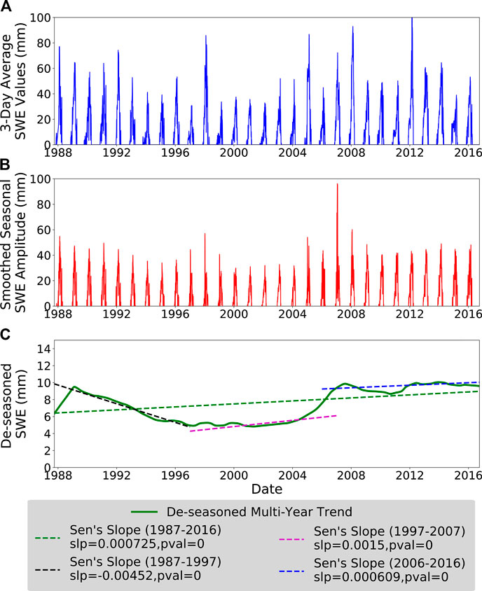
FIGURE 2. Sample location (approx. 72.06°E, 38.64°N) illustrating the (A) snow-water equivalent (SWE) time series, (B) seasonal signal to be removed, and (C) the long-term de-seasoned data. Dashed lines on (C) show fitted lines using Sen’s slope estimator over the whole dataset (green), the first decade (black), the second decade (purple), and the third decade (blue). There are strong oscillations in the fitted SWE trend based on the start and end dates chosen.
3. Results
3.1. Long-Term Snow-Water Equivalent Trends
Aggregate trends over the entirety of HMA are slightly negative (sum: −55.5 mm/yr, average: −0.01%) over 3,618 km2× 103 km2, including only trends with p < 0.05 and areas at least 500 m above sea level). While the aggregate trends appear to be small, we emphasize that trends are measured over 9.75 km2 grid cells, and represent a snow-water storage loss of 5.41 m3 × 105 m3 of water per year (Figure 3).
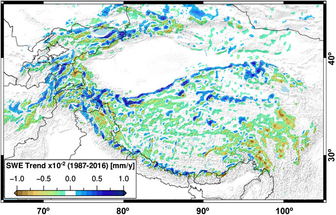
FIGURE 3. Annual snow-water equivalent (SWE) trends (1987–2016) for High Mountain Asia (HMA). There is no spatially coherent SWE trend throughout HMA, but rather several 100 km2 × 100 km2 or larger regions with similar characteristics (Fujita and Nuimura, 2011; Smith and Bookhagen, 2018; Wang et al., 2018). Large-scale negative SWE trends are observed in the Tien Shan and Pamir Mountains in western HMA, and at the eastern margin of the Tibetan plateau. The Kunlun Shan, Karakoram, and western Himalaya are characterized by positive SWEs trends.
It is clear that SWE trends are spatially diverse—positive SWE trends are concentrated in the Karakoram, Pamir, Kunlun Shan, and the high Himalaya (Figures 3 and 4A–D). The most negative trends are concentrated in the south-eastern Tibetan Plateau (Figures 4E,F), at the headwaters of the Yangtze, Salween, and Mekong rivers. There also exist many small-scale features; for example, there are clear alternating positive-negative SWE trend patterns along the front of the Himalaya. While there are multiple possible causes for such small-scale variability, the extreme topography and the microclimates it creates can drastically alter snow-loading and snow-water storage on nearby slopes—particularly when there are large differences in the sun exposure and overall aspect of neighboring slopes (Supplemental Figures S1–S5).
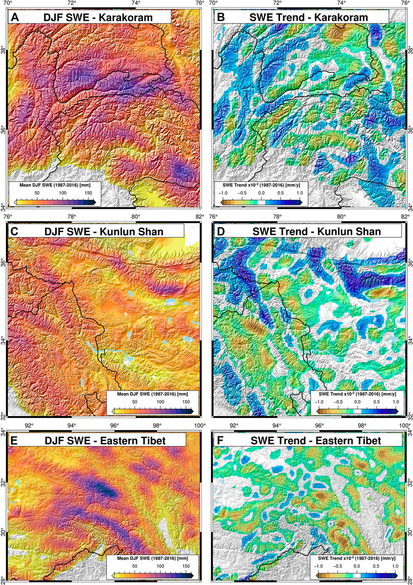
FIGURE 4. Regional zoom maps (see Figure 1 for locations). Average December-January-February (DJF) snow-water equivalent (SWE) (left column) and annual SWE trends (1987–2016, right column) for the (A,B) Karakoram-Pamir, (C,D) Kunlun Shan, and (E,F) Eastern Tibetan regions. Regional SWE trends show clear differences in magnitudes and directions: high SWE areas in the (A) Karakoram and Pamir Mountains have a wide range of trends, but overall more negative trends in high SWE areas. The (B) Kunlun Shan has lower average SWE, but stronger positive trends. (E) Eastern Tibet has high SWE with overall strongly negative SWE trends.
3.2. Seasonal Snow-Water Equivalent Trends
When the SWE data are further divided into seasonal components, clear differences in trend direction and magnitude appear (Figure 5). Strong positive winter (December-January-February) trends are visible in most of the highest peaks of HMA—running along the Himalaya, into the Pamir-Karakoram-Kunlun Shan region, as well as through the Tien Shan. These positive trends are visible through the spring (March-April-May) and fall (September-October-November) seasons as well; the only region, however, to maintain positive trends through the full year and in each seasonal slice is the Karakoram-Kunlun Shan region, which has been noted for glacier stability and growth in recent years (Hewitt, 2005; Kääb et al., 2012; Kapnick et al., 2014; Treichler et al., 2019; Shean et al., 2020). These positive trends are offset by large negative SWE trends in lower-elevation regions of HMA and along the eastern edge of the Tibetan Plateau which has seen rapidly decreasing SWE—particularly in the December-January-February and September-October-November periods (Figure 5).
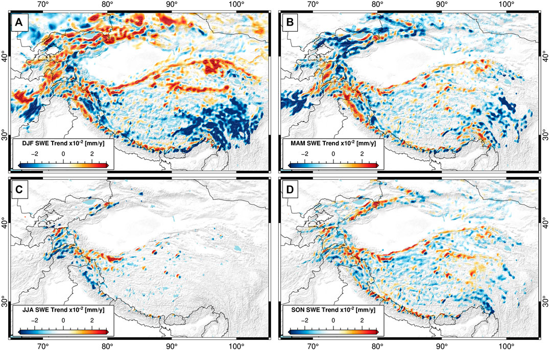
FIGURE 5. Seasonal components of snow-water equivalent (SWE) trend (1987–2016). (A) December-January-February (DJF), (B) March-April-May (MAM), (C) June-July-August (JJA), and (D) September-October-November (SON) trends all have distinct spatial patterns. Note that the magnitude scaling of the seasonal trends is three times as large as that of the annual trends (see Figure 3). The Karakoram-Kunlun Shan is the only region to maintain large-scale positive SWE trends in the summer months.
3.3. Magnitude Variations in Snow-Water Equivalent Trends
To further explore the dynamics of SWE trends in HMA, we have performed a second set of regressions using monthly SWE percentiles (Figure 6). In short, we calculate the 10th, 25th, 50th, 75th, and 90th percentile SWE value at each pixel over each month using daily-averaged SWE data (October 1987–September 2016), remove the long-term monthly mean value for each given month to reduce the impacts of seasonality, and perform regressions through each SWE percentile separately. This yields a set of SWE trend results based on only the lowest (e.g., 10th percentile) or highest (e.g., 90th percentile) SWE value for each month.
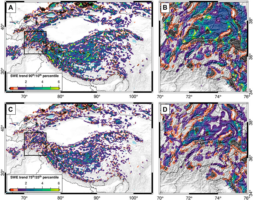
FIGURE 6. Ratios of trends in (A,B) 90th/10th percentile snow-water equivalent (SWE) and (C,D) 75th/25th percentile SWE. Panels (B,D) show zoom in box over the Karakoram, with 100 mm average December-January-February SWE contour line in thick black. Positive (e.g., blue to green) values indicate that the trend in 90th (75th) percentile SWE values is larger than the trend in 10th (25th) percentile SWE values, and that both trends have the same direction. Orange and red areas have higher 10th (25th) percentile trends than 90th (75th). Black areas indicate a reversal of trend between the 90th/10th (75th/25th) percentiles. The vast majority of High Mountain Asia—in both positive and negative SWE trend areas (see Figure 3)—has steeper trends in high-percentile SWE than in low-percentile SWE.
When the SWE trend magnitudes at each percentile are compared, differences between high- and low-percentile trends are apparent (Figure 6). In almost all cases, the trends in high-percentile SWE are steeper than those in low-percentile SWE. In positive SWE-trend regions, this indicates that high SWE amounts are becoming relatively more frequent. For example, along the border of India and Pakistan, positive SWE-trend regions (see Figure 3) have a more than six-fold higher trends in 90th percentile monthly SWE than in 10th percentile SWE, indicating a drastic increase in monthly high-SWE day frequency or magnitude. This could be due to the increased strength of the Winter Westerlies, which has been previously reported (Cannon et al., 2016b). In contrast, positive SWE-trend areas in the Pamir have higher 10th percentile magnitudes than 90th, indicating a that positive SWE trends are driven by increases in low-magnitude SWE rather than in high-magnitude SWE.
In the majority of HMA, however, SWE trends are negative (Figure 3). Thus, the high 90th/10th (75th/25th) percentile trend ratios indicate that declines in SWE have been steeper in the higher end of the monthly SWE distribution, and that high-SWE values are becoming less common overall. This agrees well with previous research, which points to overall increasing temperatures in HMA, particularly on the Tibetan Plateau (e.g., Wang et al., 2018).
4. Discussion
4.1. Comparison With Previous Work
Previous work by Smith and Bookhagen (2018) used data at 0.25° × 0.25° spatial resolution from only the SSMI-series of satellites (1987–2009) to establish trends in SWE over HMA. The higher spatial resolution data used in this study yields only slight differences in SWE trend when the same period (e.g., 1987–2009) is considered. However, there are clear differences in the trends presented by Smith and Bookhagen (2018) and those shown in Figure 3, which are due to the difference in analysis time window. To test the sensitivity of SWE trends to the analysis window, we first break our dataset into three decade-long slices, as seen in Figure 7.
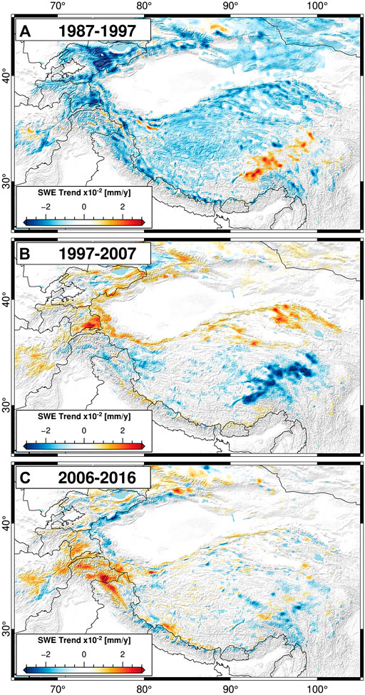
FIGURE 7. Annual snow-water equivalent (SWE) trends from (A) 1987–1997, (B) 1997–2007, and (C) 2006–2016. There are stark differences in the spatial distribution of SWE trends depending on the decade chosen. In particular, the trends in the early part of the time series (1987–1997) are significantly more negative than SWE trends over the past two decades. Note that the magnitude scaling of the decadal trends is three times as large as that of the long-term annual trends (1987–2016, see Figure 3).
It is clear that SWE trends are highly variable in time. The long-term reversal from negative to positive SWE trends seen in Figure 7, however, is supported by analysis of other related climate variables. Previous work has noted changes in regional precipitation and temperature patterns (e.g., Archer and Fowler, 2004; Yao et al., 2012; Palazzi et al., 2013; Lutz et al., 2014; Cannon et al., 2016a, Cannon et al., 2016b; Zhang et al., 2017; Wang et al., 2018; Treichler et al., 2019; Norris et al., 2020) and increases in high-elevation snowcover (Kapnick et al., 2014; Tahir et al., 2015) in recent years. Furthermore, Treichler et al. (2019) showed that increasing lake levels on the Tibetan Plateau are strongly correlated with regions of increased precipitation; modeled precipitation data suggest stepwise increases in mean annual precipitation on the Tibetan Plateau between the ∼1980s–1990s and 2000s–onwards (e.g., Kääb et al., 2018).
Recent analysis also indicates that the timing of the snowmelt season has changed over the past decades (Smith et al., 2017). While the long-term trends (1987–2016) were found to be generally negative (e.g., earlier and more rapid snowmelt), recent trends (e.g., 2004–2016) were found to be much more positive (later and slower onset of snowmelt) (Smith et al., 2017). It is therefore possible that there has been a reversal of the long-term losses in SWE storage in HMA; however, it is not clear if this is a temporary or long-term shift in the snow dynamics of HMA.
4.2. Sliding Window and Spatio-Temporal Trend Analysis
The timing and magnitude of SWE trend variability can be further explored by performing the same trend analysis on a set of time windows and start dates. We use time windows of 5, 10, 15, 20, 25, and 29 years, along with each possible combination of start years (e.g., 1987–2011) to examine changes in SWE trends through time (Figure 8).
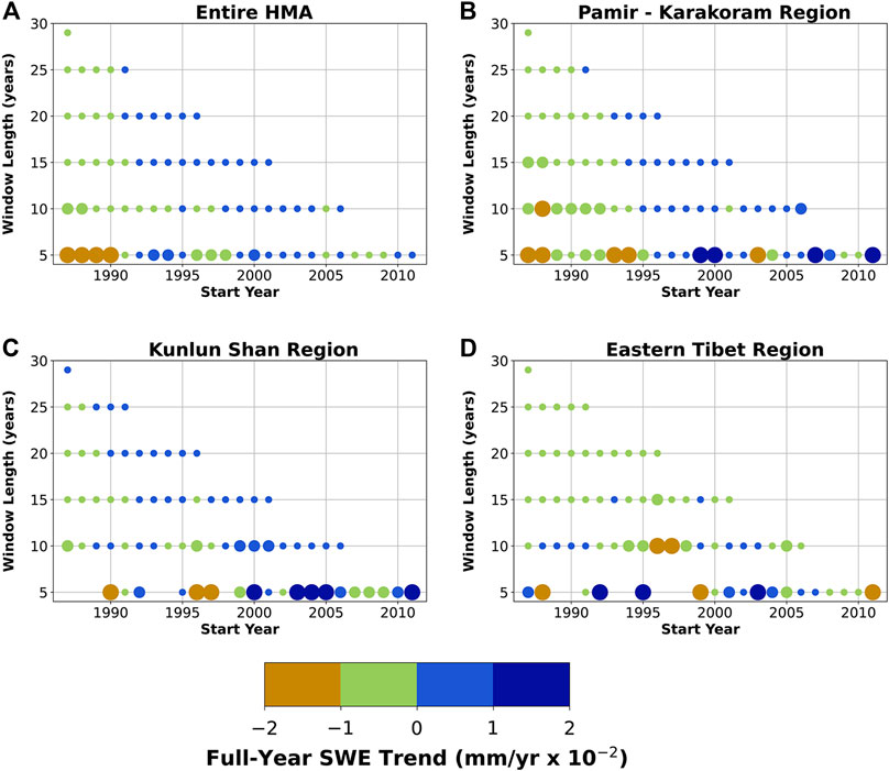
FIGURE 8. Impact of window length on measured annual snow-water equivalent (SWE) trends. Trends calculated over (A) the entire study area, (B) the Pamir-Karakoram, (C) Kunlun Shan, and (D) Eastern Tibetan regions (see Figures 1 and 4). Each dot represents averaged trends over a single window size (5–29 years) and start year (1987–2011) combination. Only statistically significant trends (p < 0.05) are included in this analysis. Larger dots indicate positive or negative trends larger than
Long-term (>25 years) SWE trends are generally negative; these trends also correspond to a particularly negative period of short-term trends starting in the late 1980s (Figure 8). More recent trends (e.g., 15–20 years) are generally positive starting in the early 1990s. One possible explanation for this phenomena is the previously proposed large-scale changes in regional precipitation over the past decades (e.g., Kääb et al., 2018). However, the impacts of changes in temperature cannot be ruled out—increasing regional temperatures can have highly variable positive and negative impacts on snow-water storage, for example, by enhancing atmospheric water content, snow density, and snowmelt rates.
There also exist strong regional variations in windowed trends (Figures 8B–D), driven by differences in climatic conditions, major weather systems, snow accumulation and ablation regimes, and dust and aerosol melt forcing between regions (Fujita, 2008; Kaspari et al., 2014; Sarangi et al., 2019). Generally positive SWE trends in the Kunlun Shan region are contrasted by mixed trends in the Karakoram, and majority negative trends in Eastern Tibet (Figures 3 and 4).
4.3. Relationship to Regional Glacier Changes
Many recent studies have investigated changes in HMA’s glaciers using a range of satellite (Bolch et al., 2012; Kääb et al., 2012; Loomis et al., 2019; Treichler et al., 2019; Shean et al., 2020) and modeling (Kapnick et al., 2014; Rounce et al., 2019) approaches to derive spatial patterns in glacier gains and losses. Using the Randolph Glacier Inventory (Arendt et al., 2015), we can measure the areal extent of glaciers within each passive microwave pixel, and—where glaciers are large enough—derive SWE trends over only glaciated areas, defined here as areas with at least 10% glacier coverage (Figure 9).
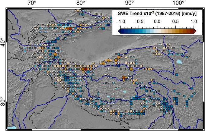
FIGURE 9. Snow-water equivalent (SWE) trends and glacier areas aggregated into 50 km × 50 km boxes. Positive (negative) trends are symbolized as circles (squares), and sized logarithmically by total glacier area within each 50 km × 50 km aggregation window, from 1 to 1,500 km2. Blue outlines show major watersheds (Lehner and Grill, 2013). There are clear positive SWE trends over the heavily glaciated Karakoram-Kunlun Shan region, which are contrasted by negative SWE trends throughout much of the rest of High Mountain Asia.
In general, SWE trends over glaciated terrain are negative, outside of parts of the Tien Shan, Karakoram, and Kunlun Shan. Areas with positive SWE trends agree well with regions of positive glacier mass balance, as presented by Shean et al. (2020) and Treichler et al. (2019). While there are many factors that influence glacier dynamics, it is likely that changes in snowfall are one of the key drivers of glacier mass gain and loss over HMA (Fujita, 2008; Fujita and Nuimura, 2011; Kapnick et al., 2014).
4.4. Data Caveats
It is important to mention caveats to the trend analysis presented in this study. The largest caveat is that passive microwave SWE estimates are often uncertain—especially over large and complex regions such as HMA (Kelly, 2009; Takala et al., 2011; Smith and Bookhagen, 2016). We also cannot rule out the impacts of both natural seasonality and regional temperature changes on snow densities, which could also modify passive microwave SWE estimates over the course of our time series, and thus are part of the trends that we present as changes in SWE in this study (Judson and Doesken, 2000; Chen et al., 2011; Dai et al., 2012). The impact of seasonal oscillations in snow density is somewhat mitigated by removing the seasonal cycle from our data before trend fitting, as some of the seasonality in SWE estimates will be driven by changes in snow density. However, without a more in-depth understanding of snow-density evolution in HMA, we cannot fully constrain this part of our analysis.
Passive microwave signal saturation could bias the presented SWE trends in deep-snow areas, as previous work has suggested that passive microwave SWE estimates saturate around 200 mm of SWE (Takala et al., 2011; Vander Jagt et al., 2013; Dozier et al., 2016). In examining our dataset, we find that the vast majority of HMA is not severely impacted by passive microwave signal saturation (Figure 10); however, it is likely that passive microwave signal saturation still biases some of our trend results. In our percentile regressions, we find that SWE trends generally maintain a consistent direction between high- and low-percentiles, indicating that saturation biases don’t drastically influence SWE trend direction (Figure 6).
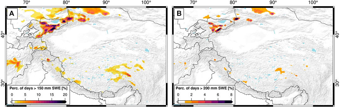
FIGURE 10. Percentage of days with snow-water equivalent (SWE) above (A) 150 mm and (B) 200 mm (1987–2016). While some areas—particularly in the Tien Shan—are impacted by SWE signal saturation, the majority of the study area should not see large signal saturation effects. Many regions where there are saturation effects also do not yield statistically significant SWE trends, and are thus not considered in our discussion of SWE trends (see Figure 3).
The third caveat is that trends are somewhat biased by the first and last values of the time series—this could also play a role in the trend reversals seen between previous studies of SWE trends in HMA (e.g., Smith and Bookhagen, 2018; Wang et al., 2018) and this study (Figures 3 and 7). We attempt to minimize this effect by using Sen’s slope estimator, which is less sensitive to the first and last values of the time series (Sen, 1968). We further attempt to mitigate the impact of the time window over which the trend is calculated by using multiple overlapping time windows and window lengths (Figure 8). Finally, we compare our results to a percentile-regression approach and find that while the magnitudes of the trends vary between percentiles and between the de-seasoned trend and percentile approaches, the trend directions found are consistent. However, snowfall can have high inter-annual variability, and we do not preclude the possibility that variations in the timing of large snowfall events between years, or shifts in the timing of snowfall and snowmelt (Smith et al., 2017) could impact estimated annual and seasonal SWE trends.
Lastly, it is important to emphasize that the trends presented here are relative to the SWE time series as estimated, and are not calibrated by in-situ measurements. While the SWE algorithms used here have been extensively validated throughout the world and have been shown to be generally reliable in low-vegetation areas (Chang et al., 1982; Chang et al., 1987; Chang et al., 1991; Chang et al., 1996; Armstrong and Brodzik, 2002; Foster et al., 2005; Derksen, 2008; Kelly, 2009; Langlois et al., 2011; Dai et al., 2015; Smith and Bookhagen, 2016), the complex topography and inaccessibility of HMA poses unique challenges for in-situ data collection. Unfortunately, calibration data of sufficient spatial and temporal resolution to properly assess our SWE estimates and trend results is not currently available in our study region. Future work could consider other approaches to constraining the estimated SWE trends, for example, by using watershed-level snowmelt runoff measurements across HMA.
5. Conclusions
The increased fidelity and spatio-temporal resolution of newly re-processed passive microwave data allows for important updates to analyses of trends in snow-water storage over HMA. While overall trends are negative, there exist large spatial and seasonal heterogeneities in snow-water storage trends. High variability in year-to-year snowfall means that trends are strongly influenced by the start and end years of any trend analysis. By using multiple overlapping time windows, we show that while long-term snow-water storage trends are majority negative, recent (e.g., past 20 years) trends are more positive. Furthermore, by using a percentile regression approach, we show that trends in high-percentile monthly SWE are generally steeper than those in low-percentile, indicating that there have been spatially diverse changes in the magnitude distributions of SWE across HMA.
Snow-water storage trends over glaciated regions generally align with previous estimates of glacier mass balance—those glaciers that are growing are highly correlated with regions of positive snow-water storage trends. However, snow-water storage trends are distinct between regions and watersheds, and can vary greatly over small distances. As the combined meltwaters from both snow and glaciers are essential to year-round water provision in the densely populated regions surrounding HMA, any changes in water storage must be considered in local and regional water planning. The high resolution and long time series data presented here allows for new and improved estimates of changes in snow-water storage that can be used to inform regional and local analyses of future water availability and watershed-level management plans.
Data Availability Statement
The passive microwave and snow-cover datasets used in this study are available from the NSIDC (Brodzik et al., 2016; Hall and Riggs, 2016). Our derived SWE trends are available on Zenodo: https://zenodo.org/record/3898517 (Smith and Bookhagen, 2020).
Author Contributions
TS and BB designed the study, TS prepared and analyzed all data, and BB contributed to the development of the methodology. Both authors wrote the manuscript led by TS.
Funding
The State of Brandenburg (Germany) through the Ministry of Science and Education and the NEXUS project supported TS for part of this study (grant to BB).
Conflict of Interest
The authors declare that the research was conducted in the absence of any commercial or financial relationships that could be construed as a potential conflict of interest.
Acknowledgments
We also acknowledge support from the BMBF ORYCS project.
Supplementary Material
The Supplementary Material for this article can be found online at: https://www.frontiersin.org/articles/10.3389/feart.2020.559175/full#supplementary-material
References
Archer, D. R., and Fowler, H. J. (2004). Spatial and temporal variations in precipitation in the upper Indus basin, global teleconnections and hydrological implications. Hydrol. Earth Syst. Sci. 8 (1), 47–61. doi:10.5194/hess-8-47-2004
Arendt, A., Bolch, T., Cogley, J., Gardner, A., Hagen, J., Hock, R., et al. (2015). “Randolph glacier inventory: a dataset of global glacier outlines,” in Global land ice measurements from space. Boulder, CO: Digital Media.
Armstrong, R. L., and Brodzik, M. J. (2002). Hemispheric-scale comparison and evaluation of passive-microwave snow algorithms. Ann. Glaciol. 34 (1), 38–44. doi:10.3189/172756402781817428
Barnett, T. P., Adam, J. C., and Lettenmaier, D. P. (2005). Potential impacts of a warming climate on water availability in snow-dominated regions. Nature 438 (7066), 303–309. doi:10.1038/nature04141
Berghuijs, W. R., Woods, R. A., and Hrachowitz, M. (2014). A precipitation shift from snow towards rain leads to a decrease in streamflow. Nat. Clim. Change 4 (7), 583–586. doi:10.1038/nclimate2246
Bolch, T., Kulkarni, A., Kääb, A., Huggel, C., Paul, F., Cogley, J. G., et al. (2012). The state and fate of himalayan glaciers. Science 336 (6079), 310–314. doi:10.1126/science.1215828
Bookhagen, B., and Burbank, D. W. (2010). Toward a complete Himalayan hydrological budget: spatiotemporal distribution of snowmelt and rainfall and their impact on river discharge. J. Geophys. Res. Earth Surf. 115 (F3), F03019. doi:10.1029/2009JF001426
Brodzik, M., Long, D., Hardman, M., Paget, A., and Armstrong, R. (2016). Measures calibrated enhanced-resolution passive microwave daily EASE-grid 2.0 brightness temperature ESDR. Boulder, CO: National Snow and Ice Data Center.
Brodzik, M. J., Billingsley, B., Haran, T., Raup, B., and Savoie, M. H. (2012). EASE-grid 2.0: incremental but significant improvements for earth-gridded data sets. Int. J. Geoinf. 1 (1), 32–45. doi:10.3390/ijgi1010032
Cannon, F., Carvalho, L. M. V., Jones, C., and Bookhagen, B. (2015). Multi-annual variations in winter westerly disturbance activity affecting the Himalaya. Clim. Dyn. 44, 441–455. doi:10.1007/s00382-014-2248-8
Cannon, F., Carvalho, L., Jones, C., Hoell, A., Norris, J., Kiladis, G., et al. (2016a). The influence of tropical forcing on extreme winter precipitation in the western Himalaya. Clim. Dynam. 48, 1213–1232. doi:10.1007/s00382-016-3137-0
Cannon, F., Carvalho, L. M., Jones, C., and Norris, J. (2016b). Winter westerly disturbance dynamics and precipitation in the western Himalaya and Karakoram: a wave-tracking approach. Theor. Appl. Climatol. 125, 27–44. doi:10.1007/s00704-015-1489-8
Chang, A. T. C., Foster, J. L., and Hall, D. K. (1987). Nimbus-7 SMMR derived global snow cover parameters. Ann. Glaciol. 9 (9), 39–44. doi:10.3189/s0260305500200736
Chang, A. T. C., Foster, J. L., and Hall, D. K. (1996). Effects of forest on the snow parameters derived from microwave measurements during the boreas winter field campaign. Hydrol. Process. 10 (12), 1565–1574. doi:10.1002/(sici)1099-1085(199612)10:12<1565::aid-hyp501>3.0.co;2-5
Chang, A. T. C., Foster, J. L., Hall, D. K, Rango, A, and Hartline, B. K. (1982). Snow water equivalent estimation by microwave radiometry. Cold Reg. Sci. Technol. 5 (3), 259–267. doi:10.1016/0165-232x(82)90019-2
Chang, A. T. C., Foster, J. L., and Rango, A. (1991). Utilization of surface cover composition to improve the microwave determination of snow water equivalent in a mountain basin. Int. J. Remote Sens. 12 (11), 2311–2319. doi:10.1080/01431169108955260
Chen, X., Wei, W., and Liu, M. (2011). Change in fresh snow density in Tianshan mountains, China. Chin. Geogr. Sci. 21 (1), 36–47. doi:10.1007/s11769-010-0434-0
Cleveland, R. B., Cleveland, W. S., McRae, J. E., and Terpenning, I. (1990). STL: a seasonal-trend decomposition procedure based on loess. J. Off. Stat. 6 (1), 3–73.
Dai, L., Che, T., and Ding, Y. (2015). Inter-calibrating SMMR, SSM/I and SSMI/S data to improve the consistency of snow-depth products in China. Rem. Sens. 7 (6), 7212–7230. doi:10.3390/rs70607212
Dai, L., Che, T., Wang, J., and Zhang, P. (2012). Snow depth and snow water equivalent estimation from AMSR-E data based on a priori snow characteristics in Xinjiang, China. Remote Sens. Environ. 127, 14–29. doi:10.1016/j.rse.2011.08.029
Derksen, C. (2008). The contribution of AMSR-E 18.7 and 10.7 GHz measurements to improved boreal forest snow water equivalent retrievals. Remote Sens. Environ. 112 (5), 2701–2710. doi:10.1016/j.rse.2008.01.001
Déry, S. J., and Brown, R. D. (2007). Recent northern hemisphere snow cover extent trends and implications for the snow-albedo feedback. Geophys. Res. Lett. 34 (22), L22504. doi:10.1029/2007gl031474
Dozier, J., Bair, E. H., and Davis, R. E. (2016). Estimating the spatial distribution of snow water equivalent in the world’s mountains. WIREs Water 3 (3), 461–474. doi:10.1002/wat2.1140
Early, D. S., and Long, D. G. (2001). Image reconstruction and enhanced resolution imaging from irregular samples. IEEE Trans. Geosci. Remote. Sens. 39 (2), 291–302. doi:10.1109/36.905237
Foster, J. L., Sun, C., Walker, J. P., Kelly, R., Chang, A., Dong, J., et al. (2005). Quantifying the uncertainty in passive microwave snow water equivalent observations. Remote Sens. Environ. 94 (2), 187–203. doi:10.1016/j.rse.2004.09.012
Fujita, K. (2008). Effect of precipitation seasonality on climatic sensitivity of glacier mass balance. Earth Planet. Sci. Lett. 276 (1), 14–19. doi:10.1016/j.epsl.2008.08.028
Fujita, K., and Nuimura, T. (2011). Spatially heterogeneous wastage of Himalayan glaciers. Proc. Natl. Acad. Sci. U.S.A. 108 (34), 14011–14014. doi:10.1073/pnas.1106242108
Gardelle, J., Berthier, E., and Arnaud, Y. (2012). Slight mass gain of Karakoram glaciers in the early twenty-first century. Nat. Geosci. 5 (5), 322–325. doi:10.1038/ngeo1450
Hall, D. K., and Riggs, G. A. (2016). MODIS/terra snow cover daily L3 global 500m SIN grid, version 6. Data Set ID: MOD10A1.
Hewitt, K. (2005). The Karakoram anomaly? Glacier expansion and the ‘elevation effect,’ Karakoram Himalaya. Mt. Res. Dev. 25 (4), 332–340. doi:10.1659/0276-4741(2005)025[0332:tkagea]2.0.co;2
Huffman, G. J., Bolvin, D. T., Nelkin, E. J., Wolff, D. B., Adler, R. F., Gu, G., et al. (2007). The TRMM multisatellite precipitation analysis (TMPA): quasi-global, multiyear, combined-sensor precipitation estimates at fine scales. J. Hydrometeorol. 8 (1), 38–55. doi:10.1175/jhm560.1
Huss, M., Bookhagen, B., Huggel, C., Jacobsen, D., Bradley, R., Clague, J., et al. (2017). Towards mountains without permanent snow and ice. Earth’s Future 5, 418–435. doi:10.1002/2016EF000514.
Immerzeel, W. W., van Beek, L. P. H., and Bierkens, M. F. P. (2010). Climate change will affect the Asian water towers. Science 328 (5984), 1382–1385. doi:10.1126/science.1183188
Judson, A., and Doesken, N. (2000). Density of freshly fallen snow in the central Rocky Mountains. Bull. Am. Meteorol. Soc. 81 (7), 1577–1588. doi:10.1175/1520-0477(2000)081<1577:doffsi>2.3.co;2
Kääb, A., Berthier, E., Nuth, C., Gardelle, J., and Arnaud, Y. (2012). Contrasting patterns of early twenty-first-century glacier mass change in the Himalayas. Nature 488 (7412), 495–498. doi:10.1038/nature11324
Kääb, A., Leinss, S., Gilbert, A., Bühler, Y., Gascoin, S., Evans, S. G., et al. (2018). Massive collapse of two glaciers in western Tibet in 2016 after surge-like instability. Nat. Geosci. 11 (2), 114–120. doi:10.1038/s41561-017-0039-7
Kapnick, S. B., Delworth, T. L., Ashfaq, M., Malyshev, S., and Milly, P. C. D. (2014). Snowfall less sensitive to warming in Karakoram than in Himalayas due to a unique seasonal cycle. Nat. Geosci. 7 (11), 834–840. doi:10.1038/ngeo2269
Kaspari, S., Painter, T. H., Gysel, M., Skiles, S. M., and Schwikowski, M. (2014). Seasonal and elevational variations of black carbon and dust in snow and ice in the Solu-Khumbu, Nepal and estimated radiative forcings. Atmos. Chem. Phys. 14 (15), 8089–8103. doi:10.5194/acp-14-8089-2014
Kelly, R. (2009). The AMSR-E snow depth algorithm: description and initial results. J. Remote Sens. Soc. Jpn. 29 (1), 307–317. doi:10.11440/rssj.29.307
Kelly, R. E., Chang, A. T., Tsang, L., and Foster, J. L. (2003). A prototype AMSR-E global snow area and snow depth algorithm. IEEE Trans. Geosci. Remote Sens. 41 (2), 230–242. doi:10.1109/tgrs.2003.809118
Kitoh, A., Endo, H., Krishna Kumar, K., Cavalcanti, I. F. A., Goswami, P., and Zhou, T. (2013). Monsoons in a changing world: a regional perspective in a global context. J. Geophys. Res. Atmos. 118 (8), 3053–3065. doi:10.1002/jgrd.50258
Langlois, A., Royer, A., Dupont, F., Roy, A., Goïta, K., and Picard, G. (2011). Improved corrections of forest effects on passive microwave satellite remote sensing of snow over boreal and subarctic regions. IEEE Trans. Geosci. Remote. Sens. 49 (10), 3824–3837. doi:10.1109/tgrs.2011.2138145
Lehner, B., and Grill, G. (2013). Global river hydrography and network routing: baseline data and new approaches to study the world’s large river systems. Hydrol. Process. 27 (15), 2171–2186. doi:10.1002/hyp.9740
Lievens, H., Demuzere, M., Marshall, H.-P., Reichle, R. H., Brucker, L., Brangers, I., et al. (2019). Snow depth variability in the northern hemisphere mountains observed from space. Nat. Commun. 10 (1), 1–12. doi:10.1038/s41467-019-12566-y
Long, D. G., and Brodzik, M. J. (2016). Optimum image formation for spaceborne microwave radiometer products. IEEE Trans. Geosci. Remote Sens. 54 (5), 2763–2779. doi:10.1109/tgrs.2015.2505677
Loomis, B. D., Richey, A. S., Arendt, A. A., Appana, R., Deweese, Y., Forman, B. A., et al. (2019). Water storage trends in High Mountain Asia. Front. Earth Sci. 7, 235. doi:10.3389/feart.2019.00235
Lutz, A. F., Immerzeel, W. W., Shrestha, A. B., and Bierkens, M. F. P. (2014). Consistent increase in High Asia’s runoff due to increasing glacier melt and precipitation. Nat. Clim. Change 4 (7), 587–592. doi:10.1038/nclimate2237
Malik, N., Bookhagen, B., and Mucha, P. J. (2016). Spatiotemporal patterns and trends of Indian monsoonal rainfall extremes. Geophys. Res. Lett. 43 (4), 1710–1717. doi:10.1002/2016gl067841
Mann, H. B. (1945). Nonparametric tests against trend. Econometrica 13, 245–259. doi:10.2307/1907187
Menon, A., Levermann, A., and Schewe, J. (2013). Enhanced future variability during India’s rainy season. Geophys. Res. Lett. 40 (12), 3242–3247. doi:10.1002/grl.50583
Norris, J., Carvalho, L. M., Jones, C., and Cannon, F. (2020). Warming and drying over the central Himalaya caused by an amplification of local mountain circulation. NPJ Clim. Atmos. Sci. 3 (1), 1–11. doi:10.1038/s41612-019-0105-5
Notarnicola, C. (2020). Hotspots of snow cover changes in global mountain regions over 2000–2018. Remote Sens. Environ. 243 (111), 781. doi:10.1016/j.rse.2020.111781
Palazzi, E., Von Hardenberg, J., and Provenzale, A. (2013). Precipitation in the Hindu-Kush Karakoram Himalaya: observations and future scenarios. J. Geophys. Res. Atmos. 118 (1), 85–100. doi:10.1029/2012jd018697
Rounce, D. R., Hock, R., and Shean, D. (2019). Glacier mass change in High Mountain Asia through 2100 using the open-source python glacier evolution model (PyGEM). Front. Earth Sci. 7, 331. doi:10.3389/feart.2019.00331
Sakai, A., and Fujita, K. (2017). Contrasting glacier responses to recent climate change in High-Mountain Asia. Sci. Rep. 7 (1), 1–8. doi:10.1038/s41598-017-14256-5
Sarangi, C. N., Qian, Y., Rittger, K., Bormann, K. J., Liu, Y., Wang, H., et al. (2019). Impact of light-absorbing particles on snow albedo darkening and associated radiative forcing over High-Mountain Asia: high-resolution WRF-chem modeling and new satellite observations. Atmos. Chem. Phys. 19 (10), 7105–7128. doi:10.5194/acp-19-7105-2019
Scherler, D., Bookhagen, B., and Strecker, M. R. (2011). Spatially variable response of Himalayan glaciers to climate change affected by debris cover. Nat. Geosci. 4 (3), 156–159. doi:10.1038/ngeo1068
Sen, P. K. (1968). Estimates of the regression coefficient based on Kendall’s Tau. J. Am. Stat. Assoc. 63 (324), 1379–1389. doi:10.1080/01621459.1968.10480934
Shean, D., Bhushan, S., Montesano, P., Rounce, D., Arendt, A., and Osmanoglu, B. (2020). A systematic, regional assessment of High Mountain Asia glacier mass balance. Front. Earth Sci. 7, 363. doi:10.3389/feart.2019.00363
Singh, D., Tsiang, M., Rajaratnam, B., and Diffenbaugh, N. S. (2014). Observed changes in extreme wet and dry spells during the south Asian summer monsoon season. Nat. Clim. Change 4 (6), 456–461. doi:10.1038/nclimate2208
Smith, T., and Bookhagen, B. (2016). Assessing uncertainty and sensor biases in passive microwave data across High Mountain Asia. Remote Sens. Environ. 181, 174–185. doi:10.1016/j.rse.2016.03.037
Smith, T., and Bookhagen, B. (2018). Changes in seasonal snow water equivalent distribution in High Mountain Asia (1987 to 2009). Sci. Adv. 4 (1), 550. doi:10.1126/sciadv.1701550
Smith, T., and Bookhagen, B. (2020). Data from: Snow variables for High Mountain Asia. doi:10.5281/zenodo.3898517
Smith, T., Bookhagen, B., and Rheinwalt, A. (2017). Spatiotemporal patterns of High Mountain Asia’s snowmelt season identified with an automated snowmelt detection algorithm, 1987–2016. Cryosphere 11 (5), 2329–2343. doi:10.5194/tc-11-2329-2017
Sorg, A., Bolch, T., Stoffel, M., Solomina, O., and Beniston, M. (2012). Climate change impacts on glaciers and runoff in Tien Shan (Central Asia). Nat. Clim. Change 2 (10), 725–731. doi:10.1038/nclimate1592
Sturm, M., Taras, B., Liston, G. E., Derksen, C., Jonas, T., and Lea, J. (2010). Estimating snow water equivalent using snow depth data and climate classes. J. Hydrometeorol. 11 (6), 1380–1394. doi:10.1175/2010jhm1202.1
Tahir, A. A., Chevallier, P., Arnaud, Y., Ashraf, M., and Bhatti, M. T. (2015). Snow cover trend and hydrological characteristics of the Astore River basin (western Himalayas) and its comparison to the Hunza basin (Karakoram region). Sci. Total Environ. 505, 748–761.doi:10.1016/j.scitotenv.2014.10.065
Takala, M., Luojus, K., Pulliainen, J., Derksen, C., Lemmetyinen, J., Kärnä, J. P., et al. (2011). Estimating northern hemisphere snow water equivalent for climate research through assimilation of space-borne radiometer data and ground-based measurements. Remote Sens. Environ. 115 (12), 3517–3529. doi:10.1016/j.rse.2011.08.014
Treichler, D., Kääb, A., Salzmann, N., and Xu, C. Y. (2019). Recent glacier and lake changes in High Mountain Asia and their relation to precipitation changes. Cryosphere 13 (11), 2977–3005. doi:10.5194/tc-13-2977-2019
Vander Jagt, B. J., Margulis, S. A., Kim, E. J., Molotch, N. P., and Molotch, N. P. (2013). The effect of spatial variability on the sensitivity of passive microwave measurements to snow water equivalent. Remote Sens. Environ. 136, 163–179. doi:10.1016/j.rse.2013.05.002
Vaughan, D. G., Comiso, J. C., Allison, I., Carrasco, J., Kaser, G., Kwok, R., et al. (2013). “Observations: cryosphere,” in Climate change 2013: the physical science basis. Contribution of Working Group I to the Fifth Assessment Report of the Intergovernmental Panel on Climate Change. Editors T. F. Stocker, D. Qin, G.-K. Plattner, M. Tignor, S. K. Allen, J. Boschung, A. Nauels, Y. Xia, V. Bex and P.M. Midgley (Cambridge, United Kingdom and New York, NY, USA: Cambridge University Press). Contribution of working group I to the fifth assessment report of the IPCC.
Wang, Z., Wu, R., and Huang, G. (2018). Low-frequency snow changes over the Tibetan plateau. Int. J. Climatol. 38 (2), 949–963. doi:10.1002/joc.5221
Wulf, H., Bookhagen, B., and Scherler, D. (2016). Differentiating between rain, snow, and glacier contributions to river discharge in the western Himalaya using remote-sensing data and distributed hydrological modeling. Adv. Water Resour. 88, 152–169. doi:10.1016/j.advwatres.2015.12.004
Yao, T., Thompson, L., Yang, W., Yu, W., Gao, Y., Guo, X., et al. (2012). Different glacier status with atmospheric circulations in Tibetan plateau and surroundings. Nat. Clim. Change 2 (9), 663–667. doi:10.1038/nclimate1580
Zhang, C., Tang, Q., and Chen, D. (2017). Recent changes in the moisture source of precipitation over the Tibetan plateau. J. Clim. 30 (5), 1807–1819. doi:10.1175/jcli-d-15-0842.1
Keywords: snow, glacier, climate change, passive microwave, special sensor microwave imager, special sensor microwave imager/sounder
Citation: Smith T and Bookhagen B (2020) Assessing Multi-Temporal Snow-Volume Trends in High Mountain Asia From 1987 to 2016 Using High-Resolution Passive Microwave Data. Front. Earth Sci. 8:559175. doi: 10.3389/feart.2020.559175
Received: 06 May 2020; Accepted: 18 August 2020;
Published: 11 September 2020.
Edited by:
Mohamed Rasmy, National Graduate Institute for Policy Studies, JapanReviewed by:
Maheswor Shrestha, Water and Energy Commission Secretariat, NepalRenguang Wu, Institute of Atmospheric Physics (CAS), China
Jeff Dozier, University of California, Santa Barbara, United States
Copyright © 2020 Smith and Bookhagen. This is an open-access article distributed under the terms of the Creative Commons Attribution License (CC BY). The use, distribution or reproduction in other forums is permitted, provided the original author(s) and the copyright owner(s) are credited and that the original publication in this journal is cited, in accordance with accepted academic practice. No use, distribution or reproduction is permitted which does not comply with these terms.
*Correspondence: Taylor Smith, dGFzbWl0aEB1bmktcG90c2RhbS5kZQ==