 P. N. Shebalin
 A. A. Baranov
- Institute of Earthquake Prediction Theory and Mathematical Geophysics, Russian Academy of Sciences, Moscow, Russia
The differential probability gain approach is used to estimate quantitatively the change in aftershock rate at various levels of ocean tides relative to the average rate model. An aftershock sequences are analyzed from two regions with high ocean tides, Kamchatka and New Zealand. The Omori-Utsu law is used to model the decay over time, hypothesizing an invariable spatial distribution. Ocean tide heights are considered rather than phases. A total of 16 sequences of M ≥6 aftershocks off Kamchatka and 15 sequences of M ≥6 aftershocks off New Zealand are examined. The heights of the ocean tides at various locations were modeled using FES 2004. Vertical stress changes due to ocean tides are here about 10–20 kPa, that is, at least several times greater than the effect due to Earth tides. An increase in aftershock rate is observed by more than two times at high water after main M ≥6 shocks in Kamchatka, with slightly less pronounced effect for the earthquakes of M = 7.8, December 15, 1971 and M = 7.8, December 5, 1997. For those two earthquakes, the maximum of the differential probability gain function is also observed at low water. For New Zealand, we also observed an increase in aftershock rate at high water after thrust type main shocks with M ≥6. After normal-faulting main shocks there was the tendency of the rate increasing at low water. For the aftershocks of the strike-slip main shocks we observed a less evident impact of the ocean tides on their rate. This suggests two main mechanisms of the impact of ocean tides on seismicity rate, an increase in pore pressure at high water, or a decrease in normal stress at low water, both resulting in a decrease of the effective friction in the fault zone.
Introduction
During last decades, the question of the effect of ocean tides on seismicity has been widely investigated. The issue of whether tidal forces really affect seismicity has been raised many times in the literature. Most of the studies established a connection between tides and seismicity, mainly on a regional scale (Klein, 1976a; Klein, 1976b; Souriau et al., 1982; Wilcock, 2001; Lin et al., 2003; Tanaka et al., 2004; Crockett et al., 2006; Stroup et al., 2007; Tanaka, 2010; Chen et al., 2012a; Datta and Kamal, 2012; Tanaka, 2012; Ide and Tanaka, 2014; Saltykov, 2014; Vergos et al., 2015; Arabelos et al., 2016; Baranov et al., 2019; Scholz et al., 2019) and others. There are also many studies linking seismicity and tides using global catalogues (Heaton, 1975; Nikolaev, 1994; Tsuruoka, et al., 1995; Tanaka et al., 2002; Cochran et al., 2004; Yurkov and Gitis, 2005; Métivier, et al., 2009; Chen et al., 2012b; Ide et al., 2016). However, many studies do not find such a correlation (Schuster, 1897; Morgan et al., 1961; Knopoff, 1964; Simpson, 1967; Shudde and Barr, 1977; Heaton, 1982; Rydelek et al., 1992; Vidale et al., 1998). A detailed review of the influence of tides on seismicity was given, for example, in (Emter, 1997).
Laboratory experiments were also conducted to study the effect of tides on seismicity (Lockner and Beeler, 1999; Beeler and Lockner, 2003). A strong correlation was found to exist between periodic stress (tides) and the occurrence of failure (earthquake) at shear stress amplitudes above approximately 0.3 MPa. Shear stress variations between 10 kPa (1 m of ocean tide load) and 0.1 MPa represent a transition region in which correlation with earthquake occurrence may occur. For amplitudes below 10 kPa (the order of the vertical component of the Earth tide), little or no correlation can be detected. These results are consistent with observations. This suggested that tidal stress amplitudes of about 3–10 kPa are required to trigger earthquakes (Hardebeck et al., 1998; Cochran et al., 2004). For example, it was shown that aftershocks after the M = 7.4 Landers event were triggered by stress increases greater than 10 kPa (Stein, 1999).
Largely since (Schuster, 1897), the tidal phases, mainly the semidiurnal phase, were studied. The amplitude-frequency properties of tides are very complex, and it is necessary to take into account the change in the amplitudes of various components of the tides. However, some studies such as (Klein, 1976a; Klein, 1976b; Souriau et al., 1982; Vidale et al., 1998; Lockner and Beeler, 1999; Wilcock, 2001; Beeler and Lockner, 2003; Stroup et al., 2007) and more recent ones (Ide and Tanaka, 2014; Ide et al., 2016; Baranov et al., 2019) analyzed tidal heights rather than tidal phases. The present study is concerned with aftershock rates after large earthquakes. This gives us high rates and high rate changes on the time scale of hours and days, compatible with the time scale of tides. In this time scale, tide height analysis seems more appropriate due to the complex tide phase structure. Actually, researchers studied the effect of Earth tides (Morgan et al., 1961; Heaton, 1975; Klein, 1976a; Klein, 1976b; Heaton, 1982; Burton, 1986; Rydelek et al., 1992; Lin et al., 2003; Métivier et al., 2009; Chen et al., 2012a; Chen et al., 2012b; Datta and Kamal, 2012; Saltykov, 2014) or the combined effect of Earth and ocean tides on seismicity (Souriau et al., 1982; Vidale et al., 1998; Tsuruoka, et al., 1995; Wilcock, 2001; Tanaka et al., 2002; Tanaka et al., 2004; Cochran et al., 2004; Stroup et al., 2007; Tanaka, 2010; Tanaka, 2012; Ide et al., 2016).
There are relatively few studies where the connection between seismicity and ocean tides was analyzed. This is due to the complexity of numerical calculations of ocean tides. Only in recent years computer programs for the numerical modeling of ocean tides have been developed. These programs were used to study the connection between ocean tides and seismicity (Crockett et al., 2006; Ide and Tanaka, 2014; Baranov et al., 2019). The result was to detect a clear connection between seismicity and ocean tides. Despite a large number of comparative studies of seismicity and tides, the relationship between aftershock rates and tides was studied in few papers (Souriau et al., 1982; Chen et al., 2012b; Datta and Kamal, 2012; Saltykov, 2014; Baranov et al., 2019). A partial dependence of aftershock rate on tidal heights (ocean and Earth tides) for normal-fault and thrust-fault earthquakes was found for the Pyrenees (Souriau et al., 1982). But for strike-slip earthquakes no statistical connection was found. The M >7 earthquakes worldwide since 1900 are more likely to occur during the 0°, 90°, 180° or 2,70° phases (i.e., earthquake-prone phases) of the semidiurnal solid Earth (M2) tidal curve (Chen et al., 2012b). Diurnal and semi-diurnal periodicities in aftershock rate (M ≥4) were found for the aftershock sequence of the Tohoku M = 9.1 earthquake of March 11, 2011 in Japan with an apparent weakening of the tidal triggering effect over time (Datta and Kamal, 2012). This suggests that large aftershocks in the fault zone of the Japan 2011 earthquake were strongly influenced by Earth tides.
Partial dependence of aftershock rates on Earth tides was also found for aftershocks of the M = 6.8 earthquake of June 21, 1996 off Kamchatka (Saltykov, 2014), and an alternative trigger mechanism was proposed for tidal effects based on an amplitude-dependent dissipation model. Another study of aftershock sequences following Kamchatka earthquakes using the method of differential probability gain, DPG (Baranov et al., 2019), demonstrated a considerable increase in the aftershock rate (by factors of two and more) at low or at high water. An increase in aftershock rate at low water corresponds to unloading of the seafloor, while high water may result in an increase of pore pressure in the fracture zone and therefore decreasing friction forces. The correlation between seismicity and tides in relation to focal mechanisms was studied by several authors. Correlation was mainly found for normal and partly for thrust slip types (Heaton, 1975; Souriau et al., 1982; Tsuruoka, et al., 1995; Tanaka et al., 2002; Cochran et al., 2004). The connection between seismicity and tides at ocean ridges were studied extensively (Wilcock, 2001; Tolstoy et al., 2002; Stroup et al., 2007; Scholz et al., 2019). A correlation between tides and seismicity was found along the Juan de Fuca Ridge (Wilcock, 2001; Tolstoy et al., 2002) and for East Pacific Rise (Stroup et al., 2007). Scholz et al. (2019) suggested pulsation of magma chambers due to vertical stress changes as a mechanism responsible for the tidal triggering of earthquakes for mid-ocean ridges.
The impact of tides on earthquakes is often explained by changes in the stress field in the fault using the Coulomb criterion (Stein, 1999; Cochran et al., 2004). Coulomb failure stress change ∆τc = ∆τ + μ(∆σn−∆P), where τ and σn are the shear stress change on the fault (assumed to be positive in the direction of slip) and the normal stress change on the fault (positive if the fault is unclamped), respectively, P is the pore pressure change in the fault, and μ is the coefficient of friction (with range 0–1). Failure is encouraged if ∆τc is positive and discouraged if negative; both increased shear and unclamping of faults facilitate failure. Thus friction threshold can be exceeded either when the normal stress is decreased or when pore pressure is increased (Klein, 1976a; Klein, 1976b; Wilcock, 2001; Tolstoy et al., 2002; Cochran et al., 2004; Stroup et al., 2007; Métivier et al., 2009). This can reflect earthquake initiation (Stein, 2004). Some authors suggested alternative mechanisms to explain the effect of tides on seismicity: nonlinear dilatancy-diffusion model (Heaton, 1982), seismic modulation by combination of different tidal waves, impacts of tidal waves occurring in resonance with the self-oscillating system of the focal zone under the influence of tidal waves (Nikolaev, 1996) or an amplitude-dependent dissipation model taking into account tidal variations in physical properties of the medium (Saltykov, 2014). The researchers used different methods to study the effect of tides on seismicity from simple visual comparison between time series of seismicity and tides to more or less sophisticated statistical methods as binomial distribution test, random distribution test, method of Chapman-Miller (Malin and Chapman, 1970), and Schuster’s test using a statistical method of Rayleigh (Schuster, 1897). Schuster’s test was described in detail in many papers (e.g., Heaton, 1975; Rydelek et al., 1992). Table 1 summarized studies of tides on seismicity using several key parameters: type of tides (Earth tides, ocean tides), tidal phases, connection with seismicity, tidal amplitude, the mechanism responsible, and the object of study.
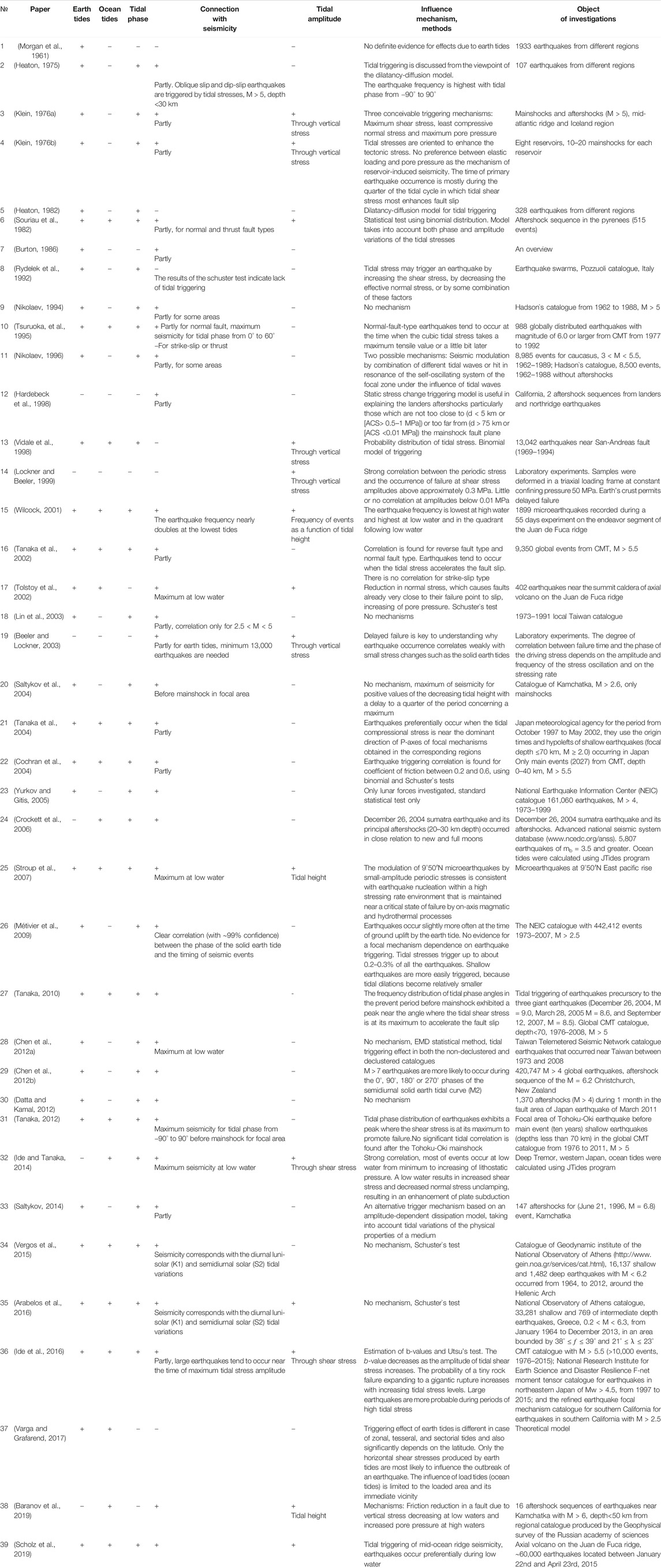
TABLE 1. A review of studies of the impact of tides on seismicity.
Why do we study the impact of ocean tides on aftershock rate using a model of tide heights?
(1) Time scales of tides and aftershock occurrence are comparable. The time-dependent distribution of aftershocks without impact of tides can be modeled.
(2) The impact of ocean tides on aftershock rates still remains a challenge (Cochran et al., 2004; Tanaka, 2012; Baranov et al., 2019).
(3) The well-known Schuster test using tide phases requires a correct catalogue declustering. Aftershocks that remain in the catalogue may alter the statistics.
(4) The impact of ocean tides on seismicity is often related to instabilities or a compliance of fault zones (Cochran et al., 2004). The aftershock zones marked by high stress perturbations perfectly fit those conditions.
(5) We concentrate here on ocean tides in areas where the amplitudes are 2 m or more (Kamchatka and New Zealand). The corresponding stress changes (10–20 kPa) are larger compared with Earth tides (Varga and Grafarend, 2017).
(6) We study ocean tide heights, not phases. Triggering of earthquakes is caused by stress changes depending on the level of tides. The frequency structure of the ocean tides is complex, and the prevailing periods may vary in time (Lyard et al., 2006).
The purpose of this publication is to assess the quantitative effect of ocean tidal heights on seismic activity and to compare these estimates for different types of faults.
Methods
Selection of Aftershock Sequences
The aftershock sequences for analysis were found using the “nearest neighbor” algorithm of Zaliapin and Ben-Zion (Zaliapin and Ben-Zion, 2013). Aftershock sequences of large earthquakes may have complex structure, with significant “splashes” of secondary aftershocks caused by large primary aftershocks. Another component of seismicity is background seismicity, which is often referred to as seismic noise. Using the “nearest neighbor” algorithm, we selected only the direct “off-spring” (Zaliapin and Ben-Zion, 2013) of the considered large earthquakes, thus minimizing the presence of secondary aftershocks and background seismicity in the selected sequences. This allowed us to model the aftershocks sequences using Omori’s law. One alternative that we used in a previous analysis (Baranov et al., 2019) is the Molchan-Dmitrieva algorithm (Molchan and Dmitrieva, 1992), which selects aftershock sequences together with secondary aftershock sub-sequences. Large aftershocks often trigger a temporary increase of activity. In such cases the Omori model may be significantly altered by this temporary activation. Direct aftershocks found using the nearest neighbor approach do not contain the secondary aftershock sequences, and thus are correctly modeled by the Omori law. Another alternative could be a stochastic declustering of the earthquake catalogue with much deeper complexity and non-uniqueness of the clusters (Varini et al., 2020). Another disadvantage of the stochastic declustering methods is their basic hypothesis that the number of aftershocks is a function of the magnitude of the corresponding main shock. This hypothesis, as was recently found, is not true (Shebalin et al., 2020).
We selected M ≥6 main shocks in the Kamchatka region, and M ≥6 events in the New Zealand region, which have offshore aftershocks. Figures 1A,B show a map of the maximum ocean tide amplitude with resolution 0.125° together with examples of offshore aftershocks for M = 7.5 (Kamchatka, June 08, 1993) and M = 7.8 (New Zealand, November 13, 2016) earthquakes. All aftershocks (as described above, we consider only direct aftershocks of the large earthquakes considered using the nearest neighbor approach), both onshore and offshore ones, were used to estimate the parameters of the Omori–Utsu law (Utsu, 1961), but only the offshore aftershocks were used to calculate the effects of ocean tides on seismicity. For selection of direct aftershocks in Kamchatka and New Zealand we used the parameters listed in Supplementaty Table S1 of (Shebalin et al., 2020).
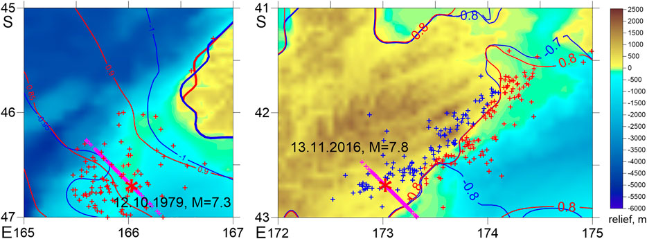
FIGURE 1. Maps of tidal heights and examples of aftershock sequences in the interval (tc, 720 h) of M = 7.3 earthquake of October 12, 1979, New Zealand (A) and M = 7.8 earthquake of November 13, 2016, New Zealand (B). Crosses mark aftershock epicenters: red in the ocean, blue on land. Red contours show maximum ocean levels, whereas blue contours show minimum levels. Colour scale shows the relief (m) with respect to sea level.
The Magnitude of Completeness Magnitude Mc and Time of Completeness tc
The catalogue completeness usually decreases after large earthquakes (Helmstetter et al., 2006; Hainzl, 2016; Shebalin and Baranov, 2017). For each aftershock sequence we began by estimating the magnitude of completeness Mc using data in the interval (tc, 1 month) after the main shock by the MBS method (Cao and Gao, 2002; Wossner and Wiemer, 2005) and tc = 1 h. At this stage we disregarded data within first 6 h after the main shocks, where which the catalogue usually remains incomplete even for relatively large magnitudes. The MBS method allows one to detect the frequently observed effect of the lack of low-magnitude aftershocks during the first few hours and sometimes days after a large earthquake, not detectable by the Maximum Curvature technique (Wiemer and Wyss, 2000), see the example in Figure 2. Then, with the preliminary value of Mc, we found tc using the equation (Helmstetter et al., 2006) Mc = Mm−4.5−0.75 log10 (tc), where Mm is the mainshock magnitude. The next step was to find the final value Mc using the same MBS technique, but with the new value of tc. In the following analysis we omit the interval (0, tc) after the main shocks.
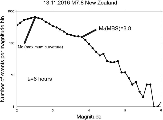
FIGURE 2. Diagram of the magnitude of completeness Mc using data in the interval (tc, 1 month) after the main shock (New Zealand, M = 7.8, November 13, 2016).
Modelling the Aftershock Rates
We model aftershock rates
where t is the time after the main shock, and c, p, and K are parameters. We estimated the parameters using aftershocks with M ≥ Mc in an interval (tc, 720 h) with the Bayesian approach (Holschneider et al., 2012), assuming that c and p are homogeneous. Figure 3 shows an example of the posterior distribution of (c, p) Bayesian estimates. We subdivide the aftershock zone into 0.2° × 0.2°boxes. The interval (tc, 720 h) is divided in subintervals of 0.2 h. Supposing the c-value and the p-value are equal in all boxes, we calculated the modeled rates of the aftershocks λij, where i is the index of spatial box, and j the time subinterval:
where
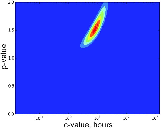
FIGURE 3. The posterior distribution of the c and p values for Bayesian estimates (Holschneider et al., 2012) for aftershocks of the M = 7.8 earthquake of December 5, 1997 in Kamchatka. Light-blue area corresponds to the 95% quantile.
Modeling Tide Heights
Real ocean tides can be as high as 12–18 m in some bays. The tidal amplitudes can reach 2 m near the Pacific coast of Kamchatka and the coast of New Zealand, producing a pressure contrast of approximately 20 kPa. The elastic response of the solid Earth to the ocean load is obtained by convolution of seawater mass distribution using FES 2004 program (http://www.aviso.altimetry.fr/). FES 2004 gives tide height at a specified point at a specified time instant (Lyard et al., 2006). The program is based on the solution of tidal barotropic equations by finite elements (triangles) on a global element grid (∼1 million elements). It uses numerical models of ocean bottom topography and shoreline (Le Provost et al., 1994; Le Provost et al., 1998). The program can compute 15 main tidal components on a 1/8° grid (amplitudes and phases), as well as 28 additional tidal components. The presence of ice is incorporated for polar regions. The accuracy is within a few centimeters for open ocean and within 10 cm for offshore areas. The grid is not uniform, being denser near the shore and less detailed in the open ocean, according to Le Provost’s criterion (Le Provost and Vincent, 1986). The program requires an input file that contains site coordinates and times in hours as measured from January 1, 1985. The program uses the sites as specified in the input file to yield tide heights at a required time instant. If a point is on land, the value is −9999. Using the FES 2004 software we modelled the heights hij of the ocean tides in each spatio-temporal volume. Next, we built a map of maximum amplitudes of ocean tides for the entire world. This map was calculated using a program of our own, Amplitude. The program iterates over the coordinates of latitude and longitude at steps of 0.125°. For each point of the mesh, the program generates a time series for a year with time step 1 min. Then, for each time series, the FES 2004 program is launched, which calculates the tide height at a given point for the annual interval and finds the maximum tide amplitude at the point. Thus, a grid is obtained where for each point the maximum amplitude of ocean tide is found. Figure 4 shows the map of the maximum ocean tide amplitude with resolution 0.125° for the entire world. New Zealand and Kamchatka that we deal with here are regions with large ocean tide amplitudes.
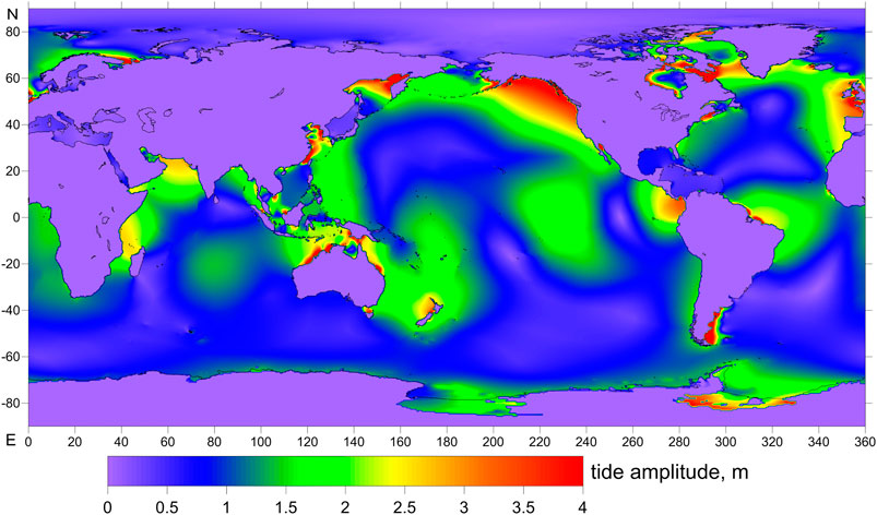
FIGURE 4. A global map of ocean tide amplitude. The colour scale shows the maximum amplitude of the ocean tide, m.
Differential Probability Gains
The ocean tide height can be considered as a parameter controlling the relative changes of seismicity rates. If a correlation between ocean tides and seismicity rates exists, then it is possible to calculate what is the average change of the rates relative to an average model, at specific values of the control parameter (Figure 5A). The differential probability gain (DPG) function (Shebalin et al., 2012; Shebalin et al., 2014) is defined as the ratio of the actual number of seismic events to the number expected on the average model. It is a function of the control parameter. Here we estimate a smoothed differential probability gain function g(h) using ranges of the control parameter with constant width dh:
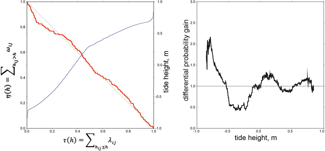
FIGURE 5. An example of the differential probability gain function. Aftershocks of the M = 6.3 earthquake of June 21, 1992 in New Zealand. A) Error diagram (red line),
Here,
In order to check if our results could have been obtained by chance, we estimated the confidence interval of the DPG estimates. For each aftershock sequence we generated 10,000 random synthetic catalogues that satisfy the Omori-Utsu law with parameters determined from the real catalogue, and repeated the procedure for determining the DPG with each synthetic catalogue. Synthetic catalogues were constructed in a standard way for a non-stationary Poisson point process with successive times found using a random number generator:
where
Seismic Data
We investigated 16 aftershocks sequences of shallow earthquakes off Kamchatka, 1971–2013 (Table 2, Figure 6A). We used seismic data from the earthquake catalogue produced by the Kamchatka Branch of the Geophysical Survey of the Russian Academy of Sciences (Chebrov et al., 2016) for the period between 1962 and 2016 (http://www.emsd.ru/sdis/earthquake/catalogue/catalogue.php). Most of the main shocks are thrust events (Figure 6A; Table 2). For New Zealand we considered aftershock sequences of 15 large (M ≥ 6) earthquakes that had at least 100 aftershocks, near New Zealand, 1979–2016 (aftershocks hypocenter data of GeoNet, Earthquake Commission and GNS Science of New Zealand, available at: http://quakesearch.geonet.org.nz; Table 3, Figure 6B). Tables 2,3 show the main parameters of these aftershock sequences.
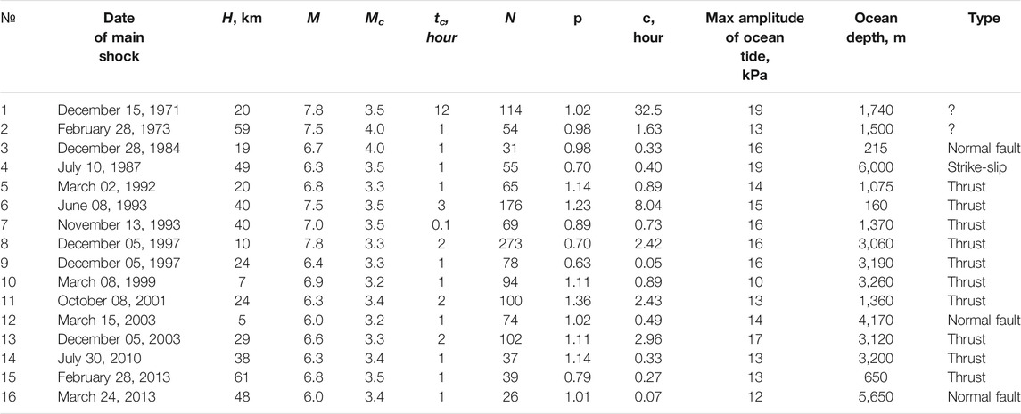
TABLE 2. The main parameters of the aftershock sequences for Kamchatka region. H denotes the main shock depth of focus; M is the mainshock magnitude; N denotes the number of M ≥ Mc aftershocks in the interval (tc, 720 h) measured from the main shock time; the maximum amplitude of ocean tide in the interval (tc, 720 h) measured from main shock time was converted to pressure, kPa; ocean depth at the epicentre of main event, m; type indicates the focal mechanism of the main event.
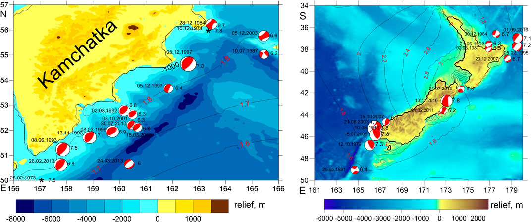
FIGURE 6. Maps of M ≥ 6 main shocks for Kamchatka, 1971–2013 (A) and New Zealand, 1979–2016 (B). The colour scale shows the relief (m) with respect to sea level; black contours with red labels show maximum amplitude of the ocean tide, m. The mainshock fault-plane solutions were taken from the Global Centroid-Moment-Tensor catalogue (Ekström et al., 2012); epicentres prior to 1976 are not reported in Global Centroid-Moment-Tensor, and they are marked by asterisks.
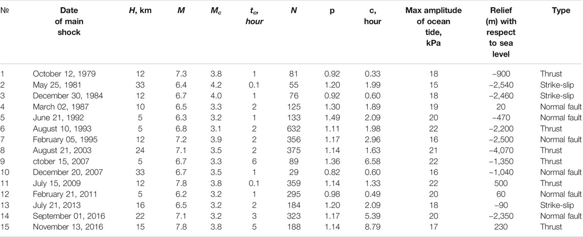
TABLE 3. The main parameters of the aftershock sequences for New Zealand. H denotes the mainshock depth of focus; M is the mainshock magnitude (magnitude ML as converted from energy class in Table 2); N denotes the number of M ≥ MC aftershocks in the interval (tc, 720 h) measured from the mainshock time; the maximum amplitude of ocean tide in the interval (tc, 720 h) measured from mainshock time was converted to pressure, kPa; relief at the epicentre of main event (m) with respect to sea level; type indicates the focal mechanism of the main event.
Figures 6A,B show a map of maximum ocean tide amplitude with resolution 0.125°. For Kamchatka near the coast, the amplitude of the ocean tides reaches 2 m, whereas for New Zealand it varies between 1.4 and 3 m, occasionally more. In Kamchatka all mainshock epicenters lie in the ocean, while for New Zealand some of the main shocks are on land, having a sufficient number of aftershocks in the ocean. Next, the quality of the catalogue for New Zealand is better, the magnitude of completeness Mc is generally smaller, and this generally results in a larger number of aftershocks to study and produces a better statistical significance of results compared with Kamchatka. The quality of hypocenter location in the catalogues is not important for our analysis. The spatial variation of the tide heights in all considered aftershock areas do not exceed 0.01 m in Kamchatka, and 0.02 m except earthquakes of 1993 and November 2016 in New Zealand; for those two earthquakes the spatial variation is about 0.07 m (Figure 1). The accuracy of the determinations of times of events (s) is very high when considered in relation to the time scale of tides (h).
Results
Aftershock sequences have been identified for 16 (M ≥6) events with epicenters near Kamchatka (see Figure 6A; Table 2) and 15 (M ≥6) events with epicenters near New Zealand (see Figure 6B; Table 3) using the methods described above. For these sequences we estimated Mc and tc as described in Section “Magnitude of completeness Mc and time of completeness tc”, and used these parameters to estimate с and p in 1 as described in Section “Modelling the aftershock rates” using data during the first month after the main shocks (Tables 2, 3). Then for rectangular 0.2° × 0.2° boxes in the ocean we estimated the modeled aftershock rates
The Kamchatka Region
Figure 7 shows differential probability gain functions for four large earthquakes (M = 6.7, December 28, 1984; M = 6.3, July 10, 1987; M = 6.8, March 2, 1992; M = 6.8, February 28, 2013). Although the differential probability gain function shape may vary from one sequence to another, all examples demonstrate a clear increase of the function at high water (>0.5 m). A similar effect is observed for all sequences, with slightly less pronounced effect for the earthquakes of M = 7.8, December 15, 1971 and M = 7.8, December 5, 1997 (Figure 8). For those two earthquakes, the maximum of the DPG function is also observed at low water (near −1 m). We have constructed also the integral differential probability gain function for Kamchatka (Figure 9). Eq. 2 was applied to all spatial boxes and time spans corresponding to several earthquakes. This analysis shows a clear maximum impact of the ocean tides at high water (>0.5 m).
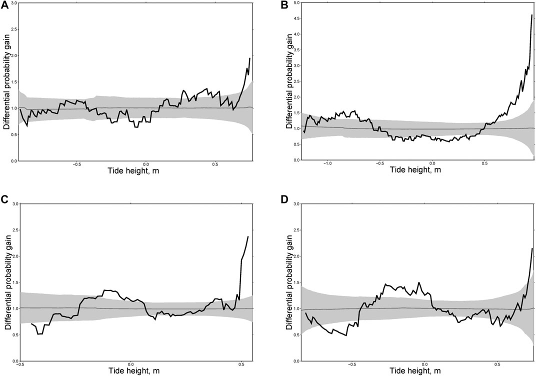
FIGURE 7. Differential probability gain functions for four aftershock sequences for Kamchatka following the earthquakes of M = 6.7, December 28, 1984 (A); M = 6.3, July 10, 1987 (B); M = 6.8, March 2, 1992 (C); M = 6.8, February 28, 2013 (D). Solid line shows values of g, the straight line marks the level 1.0.
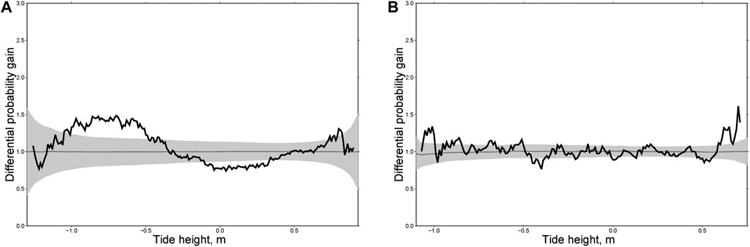
FIGURE 8. Differential probability gain functions for two aftershock sequences in Kamchatka following the earthquakes of M = 7.8, December 15, 1971 (A) and M = 7.8, December 5, 1997 (B).
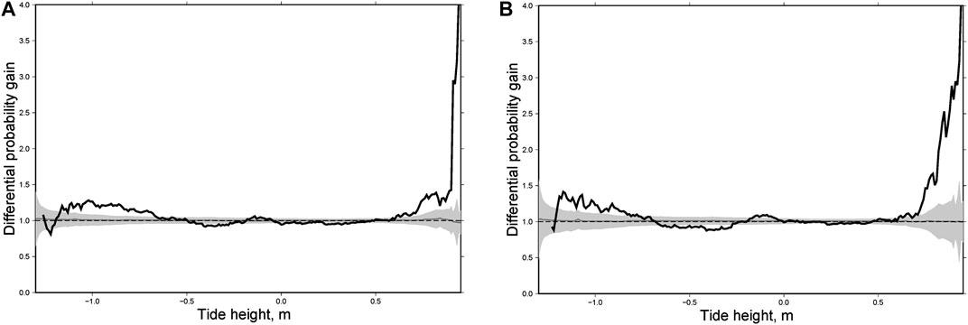
FIGURE 9. Integral differential probability gain function for Kamchatka: all 16 aftershock sequences (A) and 14 sequences without those for the M = 7.8, December 15, 1971 and M = 7.8, December 5, 1997 earthquakes (B).
New Zealand
Focal mechanisms of large earthquakes in New Zealand are different: mostly normal events in the north, thrusts in the south, and strike-slip earthquakes in the middle. Accordingly, we divided the main shocks into three groups: thrust faults (Figure 10), normal faults (Figure 11) and strike-slip faults (Figure 12). For each group we calculated individual and integral differential probability gain functions as we did for the Kamchatka sequences. As can be seen from Figures 10, for thrust faults the most general phenomenon consists in an increasing rate of aftershocks at high water (>0.5 m). A similar effect was found for Kamchatka (Figures 7–9) where almost all large earthquakes considered here were of the thrust type. For normal fault type earthquakes there is no effect at high water. In contrast, we observed a maximum of DPG at low water (<−0.5 m, Figure 11). A similar effect was observed for aftershocks following the earthquakes of M = 7.8, December 15, 1971 and M = 7.8, December 5, 1997 in Kamchatka (Figure 8). For strike-slip earthquakes the maximum of DPG functions is reached at high water for all sequences (>0.5 m). At low water, high DPG values were clearly observed for aftershocks of the M = 6.5 earthquake of July 21, 2013 (<−0.5 m, Figure 12C). These results demonstrate an impact of ocean tides on seismicity in the zones of large earthquakes within a period of 30 days after them. This highlights certain limitations to the analysis. The rupture zone of a large earthquake is in an excited state, so the impact of relatively weak disturbances, such as tides, may be stronger there than in the entire region.
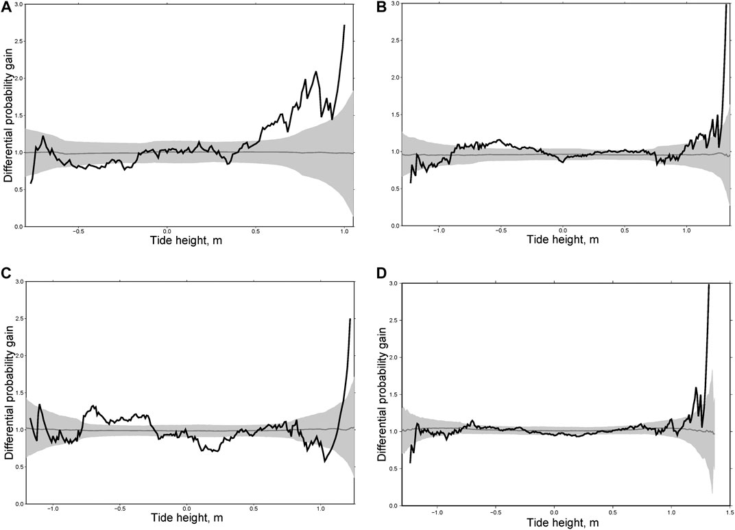
FIGURE 10. Differential probability gain functions for three aftershock sequences in New Zealand following the earthquakes of M = 7.3, October 12, 1979 (A); M = 6.8, August 10, 1993 (B); M = 7.8, July 15, 2009 (C) and the integral differential probability gain function for five aftershock sequences of thrust type earthquakes (D).
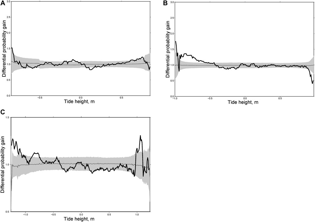
FIGURE 11. Differential probability gain functions for two aftershock sequences in New Zealand following the earthquakes of M = 6.3, June 21, 1992 (A); M = 7.8, November 13, 2016 (B); and the integral differential probability gain function for six sequences with normal slip of main shocks (C).
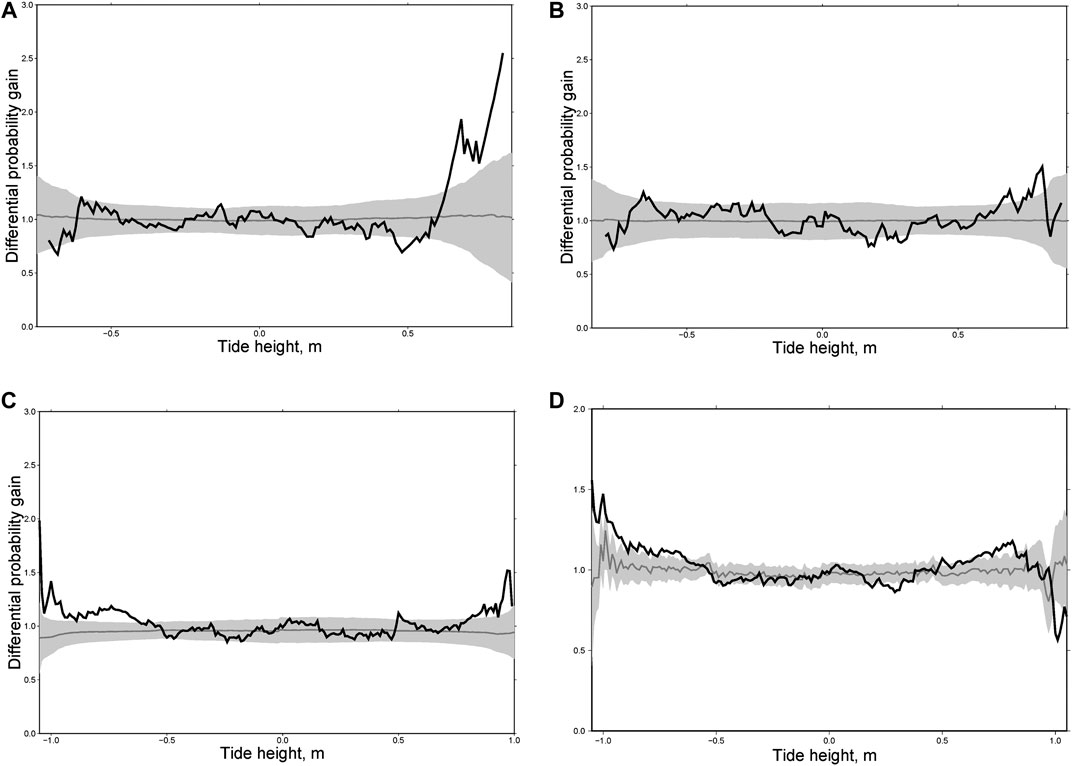
FIGURE 12. The differential probability gain functions for three aftershock sequences in New Zealand following the strike-slip earthquakes of M = 6.4, May 25, 1981 (A); M = 6.7, December 30, 1984 (B); M = 6.5, July 21, 2013 (C); and integral differential probability gain function for four sequences from strike-slip earthquakes (D).
Limitations of the Analysis
In the analysis we used a model of ocean tides. The actual tide heights may be slightly different. However, continuous direct measurements do not exist at the moment. Another shortcoming of our analysis is that we could not ascertain the role of aftershock depth. This was mostly due to lack of data below the magnitude of completeness. An unreliable depth determination for offshore earthquakes is another factor. Accordingly, the physical model of the relationships found is very preliminary.
Discussion and Conclusion
In the present study we used the differential probability gain approach (Shebalin et al., 2012; Shebalin et al., 2014) to estimate quantitatively the change in aftershock rate at various levels of ocean tides, relative to an average Omori-Utsu model that supposes no dependence on tides. The differential probability gain function is a numeric factor indicating how much the rate of aftershocks is increased or decreased on average at specific values of the tide heights. The value one indicates no impact. We consider the impact of ocean tides only, because their effect is several times larger than the effect of solid Earth tides in the regions under consideration. Variations of vertical stresses of 10–20 kPa due to ocean tides for the coast of Kamchatka and New Zealand fall within the range of the effect of stresses on seismicity according to laboratory experiments (Lockner and Beeler, 1999). Similar variations due to Earth tides at shallow depths (<50 km) are only approximately 1 kPa, i.e., one order of magnitude less (Varga and Grafarend, 2017).
We considered aftershock sequences of large (M ≥6) earthquakes off Kamchatka, 1971–2013 (16 sequences) and New Zealand, 1979–2016 (15 sequences). For all sequences we disregarded data within a few first minutes or hours after main shocks, in which the catalogue usually remains incomplete even for relatively large magnitudes. Only aftershocks with epicenters in the ocean were used. In these regions, the amplitudes of ocean tides are large, and their influence is a few times or tens of times larger than the effects of Earth tides. The observed increase in the rate of aftershocks at high and/or low water demonstrated a significant effect of ocean tides on seismicity. One important feature that distinguishes this study from most others is that we studied the heights rather than the phases of ocean tides. Moreover, the goal of this study was to find quantitative estimates of the increase in seismicity rate at specific heights of the ocean tides. The effect varies from place to place and for different focal mechanisms. The main result consists in finding a significant change in seismicity rates at tide heights more than 0.5 m relative to the baseline, positive or negative. For normal fault earthquakes the effect is stronger at low water, for thrust events mostly at high water, and for strike-slip earthquakes at high and/or low water.
Although the differential probability gains function shape may vary from one sequence to another, we observed a clear tendency of increasing aftershock rate by about two times at either low or high water. As an explanation of this effect, we can suggest friction reduction on a fault due to vertical stress decreasing at low waters and due to increased pore pressure at high waters. For normal faults an increase in aftershock rate was observed at low water, and thus the friction reduction mechanism due to the unloading of vertical stress is more likely. For thrust earthquakes, an increase in aftershock rate was observed at high water, and in that case increased pore pressure is the preferable mechanism. For strike-slip events with intermediate stresses both mechanisms can operate.
The main practical result of this study is a quantitative assessment of the effect of ocean tides on earthquake rate. Although the results were obtained for aftershocks, we may suppose that similar dependences are valid for all seismic events. Of course, this needs additional validation, but potentially opens a way to take into account ocean tides for time-dependent seismic hazard assessment.
Data Availability Statement
The raw data supporting the conclusions of this article will be made available by the authors, without undue reservation.
Author Contributions
PS provided the design and application of the differential probability gain tests. AB designed and performed calculations of the ocean tide heights.
Funding
We acknowledge the support from Russian Science Foundation Grant No. 20-17-00180.
Conflict of Interest
The authors declare that the research was conducted in the absence of any commercial or financial relationships that could be construed as a potential conflict of interest.
Acknowledgments
We acknowledge the New Zealand GeoNet project and its sponsors EQC, GNS Science and LINZ, and Kamchatka Branch of the Geophysical Survey of Russian Academy of Sciences for providing data used in this study. We are grateful to the authors of the FES 2004 for letting us use this software. We thank the reviewers for constructive comments which helped to improve the manuscript significantly.
Supplementary Material
The Supplementary Material for this article can be found online at: https://www.frontiersin.org/articles/10.3389/feart.2020.559624/full#supplementary-material.
References
Arabelos, D. N., Contadakis, M. E., Vergos, G., and Spatalas, S. (2016). Variation of the Earth tide-seismicity compliance parameter during the recent seismic activity in Fthiotida, central Greece. Ann. Geophys. 59 (1), 102. doi:10.4401/ag-6795
Baranov, A. A., Baranov, S. V., and Shebalin, P. N. (2019). A quantitative estimate of the effects of sea tides on aftershock activity: Kamchatka. J. Volcanol. Seismol. 13 (1), 56–69. doi:10.1134/S0742046319010020
Beeler, N. M., and Lockner, D. A. (2003). Why earthquakes correlate weakly with the solid Earth tides: effects of periodic stress on the rate and probability of earthquake occurrence. J. Geophys. Res. Solid Earth 108 (B8), 2156–2202. doi:10.1029/2001JB001518
Burton, P. (1986). Geophysics: is there coherence between Earth tides and earthquakes? Nature 321 (6066), 115. doi:10.1038/321115a0
Cao, A. M., and Gao, S. S. (2002). Temporal variations of seismic b-values beneath northeastern Japan Island Arc. Geophys. Res. Lett. 29, 481–482. doi:10.1029/2001GL013775
Chebrov, V. N., Droznina, S. Ya., and Senyukov, S. L. (2016). Kamchatka and the commander islands in Zemletryaseniya v Rossii v 2014 godu (Earthquakes in Russia in 2014). Obninsk, Russia: GS RAN, 60–66.
Chen, H.-J., Chen, C.-Y., Tseng, J.-H., and Wang, J.-H. (2012a). Effect of tidal triggering on seismicity in Taiwan revealed by the empirical mode decomposition method. Nat. Hazards Earth Syst. Sci. 12, 2193–2202. doi:10.5194/nhess-12-2193-2012
Chen, L., Chen, J. G., and Xu, Q. H. (2012b). Correlation between solid tides and worldwide earthquakes M C 7 since 1900. Nat. Hazards Earth Syst. Sci. 12, 587–590. doi:10.5194/nhess-12-587-2012
Cochran, E. S., Vidale, J. E., and Tanaka, S. (2004). Earth tides can trigger shallow thrust fault earthquakes. Science 306, 1164–1166. doi:10.1126/science.1103961
Crockett, R. G., Gillmore, M. G. K., Phillips, P. S., and Gilbertson, D. D. (2006). Tidal synchronicity of the December 26, 2004 Sumatran earthquake and its aftershocks. Geophys. Res. Lett. 33, L19302. doi:10.1029/2006GL027074
Datta, A., and Kamal, K. (2012). Triggering of aftershocks of the Japan 2011 earthquake by Earth tides. Curr. Sci. 102 (5), 792–796. doi:10.2307/24084467
Ekström, G., Nettles, M., and Dziewonski, A. M. (2012). The global CMT project 2004–2010: Centroid-moment tensors for 13,017 earthquakes. Phys. Earth Planet. In. 200–201, 1–9. doi:10.1016/j.pepi.2012.04.002
Emter, D. (1997). Tidal triggering of earthquakes and volcanic events. Tidal Phenomena 66, 293–309. doi:10.1007/BFb0011468
Hainzl, S. (2016). Rate-dependent incompleteness of earthquake catalogs. Seismol Res. Lett. 96 (2A), 337–344. doi:10.1785/0220150211
Hardebeck, J. L., Nazareth, J. J., and Hauksson, J. (1998). The static stress change triggering model: constraints from two southern California aftershock sequences. J. Geophys. Res. Solid Earth 103, 24427–24437. doi:10.1029/98JB00573
Heaton, T. H. (1975). Tidal triggering of earthquakes. Geophys. J. Roy. Astron. Soc. 43, 307–326. doi:10.1111/j.1365-246X.1975.tb00637.x
Heaton, T. H. (1982). Tidal triggering of earthquakes. Bull. Seismol. Soc. Am. 72, 2181–2200. doi:10.1111/j.1365-246X.1975.tb00637.x
Helmstetter, A., Kagan, Y. Y., and Jackson, D. (2006). Comparison of short-term and time-independent earthquake forecast models for southern California. Bull. Seismol. Soc. Am. 96 (1), 90–106. doi:10.1785/0120050067
Holschneider, M., Narteau, C., Shebalin, P., Peng, Z., and Schorlemmer, D. (2012). Bayesian analysis of the modified Omori law. J. Geophys. Res. 117, B05317. doi:10.1029/2011JB009054
Ide, S., and Tanaka, Y. (2014). Controls on plate motion by oscillating tidal stress: evidence from deep tremors in western Japan. Geophys. Res. Lett. 41, 3842–3850. doi:10.1002/2014GL060035
Ide, S., Yabe, S., and Tanaka, Y. (2016). Earthquake potential revealed by tidal influence on earthquake size–frequency statistics. Nat. Geosci. 9, 834–837. doi:10.1038/ngeo2796
Klein, F. W. (1976a). Earthquake swarms and the semidiurnal solid earth tide. Geophys. J. Int. 45, 245–295. doi:10.1111/j.1365-246X.1976.tb00326.x
Klein, F. W. (1976b). Tidal triggering of reservoir-associated earthquakes. Eng. Geol. 10, 197–210. doi:10.1016/0013-7952(76)90020-x
Knopoff, L. (1964). Earth tides as a triggering mechanism of earthquakes. Bull. Seismol. Soc. Am. 54, 1865–1870.
Le Provost, C., Lyard, F., Molines, J. M., Genco, M. L., and Rabilloud, F. (1998). A hydrodynamic ocean tide model improved by assimilating a satellite altimeter-derived data set. J. Geophys. Res. 103, 5513–5529. doi:10.1029/97JC01733
Le Provost, C., Genco, M. L., Lyard, F., Vincent, P., and Canceil, P. (1994). Spectroscopy of the world ocean tides from a finite element hydrodynamic model. J. Geophys. Res. 99, 777–797. doi:10.1029/94JC01381
Le Provost, C., and Vincent, P. (1986). Some tests of precision for a finite element model of ocean tides. J. Comput. Phys. 65, 273–291. doi:10.1016/0021-9991(86)90209-3
Lin, C. H., Yeh, Y. H., Chen, Y. I., Liu, J. Y., and Chen, K. J. (2003). Earthquake clustering relative to lunar phases in Taiwan. Terr. Atmos. Ocean Sci. 14, 289–298. doi:10.3319/TAO.2003.14.3.289(T)
Lockner, D. A., and Beeler, N. M. (1999). Premonitory slip and tidal triggering of earthquakes. J. Geophys. Res. 104 (B9), 20133–20151. doi:10.1029/1999JB900205
Lyard, F., Lefèvre, F., Letellier, T., and Francis, O. (2006). Modelling the global ocean tides: a modern insight from FES 2004. Ocean Dynam. 56, 394–415. doi:10.1007/s10236-006-0086-x
Malin, S. R. C., and Chapman, S. (1970). The determination of lunar daily geophysical variations by the Chapman-Miller method. Geophys. J. Roy. Astron. Soc. 19, 15–35. doi:10.1111/j.1365-246X.1970.tb06738.x
Metivier, L., de Viron, O., Conrad, C. P., Renault, S., Diament, M., and Patau, G. (2009). Evidence of earthquake triggering by the solid earth tides. Earth Planet Sci. Lett. 278, 370–375. doi:10.1016/j.epsl.2008.12.024
Molchan, G. M., and Dmitrieva, O. E. (1992). Aftershock identification: methods and new approaches. Geophys. J. Int. 109, 501–516. doi:10.1111/j.1365-246X.1992.tb00113.x
Molchan, G. M. (1991). Structure of optimal strategies in earthquake prediction. Tectonophysics 193, 267–276. doi:10.1016/0040-1951(91)90336-Q
Morgan, W. J., Stoner, J. O., and Dicke, R. H. (1961). Periodicity of earthquakes and the invariance of the gravitational constant. J. Geophys. Res. 66 (11), 3831–3843. doi:10.1029/JZ066i011p03831
Nikolaev, V. A. (1996). Relationships between seismicity and the phases of multiple and difference tidal waves. Dokl. Akad. Nauk. 349 (3), 389–394.
Nikolaev, V. A. (1994). The response of large earthquakes to the phases of earth tides. Izvestiya Phys. Solid Earth 11, 49–55.
Rydelek, P. A., Sacks, I. S., and Scarpa, R. (1992). On tidal triggering of earthquakes at Campi Flegrei. Italy. Geophys. J. Int. 109, 125–137. doi:10.1111/j.1365-246X.1992.tb00083.x
Saltykov, V. A., Ivanov, V. V., and Kugaenko, Y. A. (2004). The action of earth tides on seismicity prior to the Mw 7.0 November 13, 1993, Kamchatka earthquake. Izvestiya Phys. Solid Earth 7, 25–34.
Saltykov, V. A. (2014). Tidal effects and amplitude-dependent dissipation in seismicity. Fizicheskaya Mezomekhanika 17, 103–110.
Scholz, C. H., Tan, Y. J., and Albino, F. (2019). The mechanism of tidal triggering of earthquakes at mid-ocean ridges. Nat. Commun. 10, 2526. doi:10.1038/s41467-019-10605-2
Schuster, A. (1897). On lunar and solar periodicities of earthquakes. Proc. Roy. Soc. Lond. 61, 455. doi:10.1098/rspl.1897.0060
Shebalin, P., and Baranov, S. (2017). Long-delayed aftershocks in New Zealand and the 2016 M 7.8 Kaikoura earthquake. Pure Appl. Geophys. 174 (10), 3751–3764. doi:10.1007/s00024-017-1608-9
Shebalin, P. N., Narteau, C., and Baranov, S. V. (2020). Earthquake productivity law. Geophys. J. Int. 222 (2), 1264–1269. doi:10.1093/gji/ggaa252
Shebalin, P. N., Narteau, C., and Holschneider, M. (2012). From alarm-based to rate-based earthquake forecast models. Bull. Seismol. Soc. Am. 102, 64–72. doi:10.1785/0120110126
Shebalin, P. N., Narteau, C., Zechar, J. D., and Holschneider, M. (2014). Combining earthquake forecasts using differential probability gains. Earth Planets Space 66, 37. doi:10.1186/1880-5981-66-37
Shudde, R. H., and Barr, D. R. (1977). An analysis of earthquake frequency data. Bull. Seismol. Soc. Am. 67, 1379–1386.
Simpson, J. F. (1967). Earth tides as a triggering mechanism for earthquakes. Earth Planet Sci. Lett. 2, 473–478. doi:10.1016/0012-821X(67)90192-6
Souriau, M., Souriau, A., and Gagnepain, J. (1982). Modeling and detecting interactions between Earth tides and earthquakes with application to an aftershock sequence in the Pyrenees. Bull. Seismol. Soc. Am. 72, 165–180.
Stein, R. S. (1999). The role of stress transfer in earthquake occurrence. Nature 402, 605–609. doi:10.1038/45144
Stein, R. S. (2004). Tidal triggering caught in the act. Science 305 (5688), 1248–1249. doi:10.1126/sciencee.1100726
Stroup, D. F., Bohnenstiehl, D. R., Tolstoy, M., Waldhauser, F., and Weekly, R. T. (2007). Pulse of the seafloor: tidal triggering of microearthquakes at 9°50′N East Pacific Rise. Geophys. Res. Lett. 34, L15301. doi:10.1029/2007GL030088
Tanaka, S., Ohtake, M., and Sato, H. (2002). Evidence for tidal triggering of earthquakes as revealed from statistical analysis of global data. J. Geophys. Res. 107 (B10), 2211. doi:10.1029/2001JB001577
Tanaka, S., Ohtake, M., and Sato, H. (2004). Tidal triggering of earthquakes in Japan related to the regional tectonic stress. Earth Planets Space 56, 511–515. doi:10.1186/BF03352510
Tanaka, S. (2010). Tidal triggering of earthquakes precursory to the recent sumatra megathrust earthquakes of December 26, 2004 (Mw 9.0), March 28, 2005 (Mw 8.6), and September 12, 2007 (Mw 8.5). Geophys. Res. Lett. 37, L02301. doi:10.1029/2009GL041581
Tanaka, S. (2012). Tidal triggering of earthquakes prior to the 2011 Tohoku-Oki earthquake (Mw 9.1). Geophys. Res. Lett. 39, L00G26. doi:10.1029/2012GL051179
Tolstoy, M., Vernon, F. L., Orcutt, J. A., and Wyatt, F. K. (2002). Breathing of the seafloor: tidal correlations of seismicity at Axial volcano. Geology 30, 503–506. doi:10.1130/0091-7613(2002)030<0503:BOTSTC>2.0.CO;2
Tsuruoka, H., Ohtake, M., and Sato, H. (1995). Statistical test of the tidal triggering of earthquakes: contribution of the ocean tide loading effect. Geophys. J. Int. 122, 183–194. doi:10.1111/j.1365-246X.1995.tb03546.x
Varga, P., and Grafarend, E. (2017). Influence of tidal forces on the triggering of seismic events. Pure Appl. Geophys. 175, 1–9. doi:10.1007/s00024-017-1563-5
Varini, E., Peresan, A., and Zhuang, J. (2020). Topological comparison between the stochastic and the nearest‐neighbor earthquake declustering methods through network analysis. J. Geophys. Res. Solid Earth 125, e2020JB019718. doi:10.1029/2020JB019718
Vergos, G. S., Arabelos, D., and Contadakis, M. E. (2015). Evidence for tidal triggering on the earthquakes of the Hellenic Arc, Greece. Phys. Chem. Earth 85–86, 210–215. doi:10.1016/j.pce.2015.02.004
Vidale, J. E., Agnew, D. C., Johnston, M. J. S., and Oppenheimer, D. H. (1998). Absence of earthquake correlation with Earth tides: an indication of high preseismic fault stress rate. J. Geophys. Res. 103 (B10), 24567–24572. doi:10.1029/98JB00594
Wiemer, S., and Wyss, M. (2000). Minimum magnitude of completeness in earthquake catalogs: examples from Alaska, the western United States, and Japan. Bull. Seismol. Soc. Am. 90, 859–869. doi:10.1785/0119990114
Wilcock, W. S. (2001). Tidal triggering of microearthquakes on the Juan de Fuca ridge. Geophys. Res. Lett. 28, 3999–4002. doi:10.1029/2001GL013370
Woessner, J., and Wiemer, S. (2005). Assessing the quality of earthquake catalogues: estimating the magnitude of completeness and its uncertainty. Bull. Seismol. Soc. Am. 95, 684–698. doi:10.1785/0120040007
Yurkov, E. F., and Gitis, V. G. (2005). On relationships between seismicity and the phases of tidal waves. Izvestiya Phys. Solid Earth 4, 4–15.
Keywords: ocean tides, Kamchatka, New Zealand, FES 2004, Omori-Utsu law, differential probability gain, pore pressure, effective friction
Citation: Shebalin PN and Baranov AA (2020) Aftershock Rate Changes at Different Ocean Tide Heights. Front. Earth Sci. 8:559624. doi: 10.3389/feart.2020.559624
Received: 06 May 2020; Accepted: 26 October 2020;
Published: 21 December 2020.
Edited by:
Antonella Peresan, Istituto Nazionale di Oceanografia e di Geofisica Sperimentale (OGS), ItalyReviewed by:
Cataldo Godano, University of Campania Luigi Vanvitelli, ItalyProsanta Kumar Khan, Indian Institute of Technology Dhanbad, India
Copyright © 2020 Shebalin and Baranov. This is an open-access article distributed under the terms of the Creative Commons Attribution License (CC BY). The use, distribution or reproduction in other forums is permitted, provided the original author(s) and the copyright owner(s) are credited and that the original publication in this journal is cited, in accordance with accepted academic practice. No use, distribution or reproduction is permitted which does not comply with these terms.
*Correspondence: A. A. Baranov, YmFyYW5vdkBpZnoucnU=