 Nazzareno Diodato
 Chiara Bertolin
 Gianni Bellocchi1,3
- 1Met European Research Observatory – International Affiliates Program of the University Corporation for Atmospheric Research, Benevento, Italy
- 2Department of Mechanical and Industrial Engineering, Faculty of Engineering, Norwegian University of Science and Technology, Trondheim, Norway
- 3Université Clermont Auvergne, INRAE, Clermont-Ferrand, France
Emerging negative trends in snow depth and cover days highlight the challenges posed by changing snow patterns around the world. They suggest that snow-dependent regions in southern Europe could be affected by these changes because the number of days with snow on the ground (DSG) determines soil processes and water-flow in rivers, streams, lakes and reservoirs. We present here the first homogeneous, annually-resolved (from October to April), multi-centennial (1681–2018 CE) DSG time-series for the Parma meteorological observatory (OBS), in northern Italy, which to date is also the longest DSG series reconstructed in the world. DSG data are in fact still poorly documented and misunderstood due to the limited and fragmentary data measurements of the past. DSG recording only began in 1938 at Parma OBS. To generate the long-term annual DSG time-series at the study site, we develop a model consistent with calibration (1938–1990 CE) and validation (1991–2018 CE) samples of observed data. We show that the variability of DSG depends on winter precipitation and air temperature, as well as on winter-spring temperature variability, suggesting that long sequences of DSG are dominated by cold air masses in years with cold weather and high variability. Modeled DSG data show a downward trend from the 19th century, in the transition period from the cold of the Little Ice Age to the warmth of modern times, followed by a more rapid decline in the five most recent decades. The DSG at Parma OBS appear to have followed over the last century trends similar to those observed throughout Eurasia and across the Northern Hemisphere, where a marked decline of snow-cover duration has been reported in the transition seasons (spring and autumn).
Introduction

Publio Virgilio Marone – Georgiche, I century B.C., Libro III (Italian translation from Latin: Clemente Bondi, 1801; our translation to English).
Every snowfall deposits its own layer on the soil surface. The timing, duration and persistence of the snowfall, which depend on climatic conditions, influence the amount of water stored in soils and its use for agriculture and other sectors such as industry, urban and rural domestic water supply (e.g., Lute et al., 2015; Barnhart et al., 2016; Wang et al., 2018a; Jennings et al., 2018). Large-scale snow-cover anomalies also cause important changes in the diabatic heating of the Earth’s surface by enhancing the fraction of solar radiation reflected away by the surface (i.e., the surface albedo), thus becoming an essential component of the terrestrial radiation balance (e.g., Cohen and Rind, 1991; Goward, 2005; Sandells and Flocco, 2014). Snow cover affects the timing and magnitude of flow peaks generated by snow melting (Wang et al., 2006). By delaying the transfer of precipitation to surface runoff and infiltration in catchment areas, it also influences flow reduction and the extent of the flow network during summer baseflow (Yarnell et al., 2010; Godsey et al., 2014).
Knowledge of past climate is an important key to understanding long-term snow-cover variability. For instance, capturing anomalously cold and snowy winters can be consistent with, and help explain, a persistence of snow cover on the surface in late spring (after Jungclaus, 2009; Handmer et al., 2012; Enzi et al., 2014). In particular, the interannual variability of the number of days of snow on the ground (DSG) is an important part of the climate signal to detect potential changes of snowfall intensity and spatial distribution of snowpack variables that may have important impacts on both the environment and the society (Changnon and Changnon, 2006; O’Gorman, 2014). Our understanding of the DSG characteristics in several regions of the world is limited because of the short records available and a poor knowledge of the complex weather and climate patterns that occur locally. In Europe, the snowfall dynamics depend on the latitude and atmospheric circulation patterns, modulated by local orographic situations (Croce et al., 2018; Kretschmer et al., 2018). Polar maritime air masses originating from over the Atlantic collide here with the polar continental air masses connected with the Asian high pressure (Bednorz, 2004). The temperature control is dominant in the transient snow regions where the mean winter temperature is slightly below, and often crosses, the melting point (Diodato and Bellocchi, 2020). The situation is different in regions where the mean winter temperature is well below 0°C, as is the case of the Alps, where increases in DSG are controlled mainly by precipitation inputs (Clark et al., 1999). At lower-elevations, DSG are instead affected principally by air temperature and only secondarily by precipitation conditions.
Data on snowfall and the persistence of snow cover on the surface are becoming increasingly important due to the high variability of snowfall rates worldwide (e.g., Davi et al., 2012), and the impact that snow cover can have on society, agriculture and water resources. A quantitative assessment of the long-term and interannual DSG variability is noticeable for the identification and framing of signals of climate change, the validation of climate models, and a better understanding of the interactions among the different spheres of the Earth system, including the geosphere, biosphere, atmosphere, hydrosphere and cryosphere (Brown, 2014). Documentary sources, usually in manuscripts or annotations in different formats, provide evidence and useful information to study the variability of the climate over historical periods (Glaser and Riemann, 2009; Dobrovolný et al., 2010). However, the quality and quantity of sources are often unevenly distributed in space and time (Bradley and Jones, 1992; Mann et al., 2000; Brázdil et al., 2005; Adamson, 2015). This is especially true for snowfall, considering that in situ continuous snow monitoring is an arduous task (De Walle and Rango, 2008) and satellite remote sensing data capturing the snow-cover evolution are limited to recent decades (e.g., Pimentel et al., 2017). Also for historical times, snow characteristics data remain still poorly documented and understood due to limited and fragmented measurements (Kunkel et al., 2016; Figure 1). One of the longest-running snowfall records is the series of Parma observatory (Parma OBS), in the Padan plain (northern Italy), where however recording of DSG only started in the winter season 1937–1938. This coincides with the setup of new measuring meteorological facilities at ground level and no longer on the tower of the OBS, the suburbs and the city center.
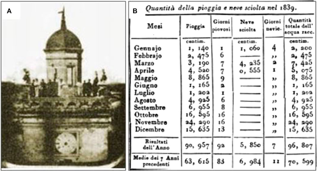
FIGURE 1. (A) The Parma meteorological observatory from a historical picture; (B) monthly summary of precipitation records (rainfall and snowfall) for the year 1839 (note the absence of recording in days with snow on the ground). Historical pictures are: (A) made freely available from Fabrizio Bonoli (University of Bologna, Italy) through the web-based content store (in Italian) of Ravenna Planetarium (http://planet.racine.ra.it/testi/astr_it.htm) [Accessed September 10, 2020]; (B) an excerpt of a printed image from Colla. (1840).
Centrally located in the Po River Basin (PRB), the Parma OBS started weather observations on 1777 thanks to the local Jesuit community with the support of the University of Parma, but only in the 20th century regular and continuous daily snowfall measurements were recorded. Diodato et al. (2020a) provided the series of monthly snowfall reconstruction in Parma over the 1777–2018 period, with the detailed analysis of metadata. In this regard, Italian regions hold among the world’s longest monthly snowfall time series (Enzi et al., 2014), going back to 1780 at Rome (Mangianti and Beltrano, 1993), 1788 at Turin (Leporati and Mercalli, 1994) and 1884 at Montevergine (Diodato, 1997). Nevertheless, Parma OBS possesses the longest continuous record, as it goes back to 1777, although we know (Camuffo and Bertolin, 2012) that meteorological observers were already active in Parma from 1654 to 1660, supported by the Grand Duke of Tuscany Ferdinand II de’ Medici (1610–1670).
The current work presents the first annually-resolved reconstruction of DSG since 1681 (i.e., the snow winter season going from October 1680 to April 1681) for the Parma OBS. A day with snow cover is a day with snow of at least 0.01 m depth observed in over 50% of an open neighboring area (UNESCO/IASH/WMO, 1970; WMO, 2008). Winter maximum number of days with snow depth matching these criteria was used to characterize snow cover duration for the purpose of this study (e.g., Falarz, 2004; Petkova et al., 2004). We first acquired a comprehensive knowledge about potential drivers of DSG in the PRB (Materials and Methods), where snowfall occurs from October to April, and then we used these factors (amounts of precipitation and air temperature) to develop a tight or “parsimonious” model for reconstructing annual DSG data over the period 1681–2018 CE (Results and Discussion). This allowed us to capture a wide range of climate variability and identify patterns of snowfall changes reported and discussed in section.
Materials and Methods
Environmental Setting and Data
Parma OBS (44° 48′ N; 10° 19′ E, 49 m a.s.l.) is located in the central part of the PRB, in the Italian administrative region Emilia-Romagna (Figure 2A). This area is surrounded by the pre-Alps to the north and by the Emiliano Apennine to the south (Figure 2B). The interaction between these morphology and weather characteristics governs the occurrence of DSG (whose measurements are available since July 1937) under different conditions. The Parma OBS (black dot in Figure 2C) outlines a separation between the snowy peaks over the northern and western pre-alpine and alpine chains and the Apennines to the south where the climate is less continental. Complex reliefs, different slope exposures, as well as various distances to sea (Figure 2B), exert highly contrasting effects on snow-cover depth, persistence and spatial extent. The colored bands in Figure 2C do explain the amplitude of sub-regional variations around the Parma OBS. For instance, south of Parma the average snow-cover duration rises up to ∼80 days year−1 in the Apennines.
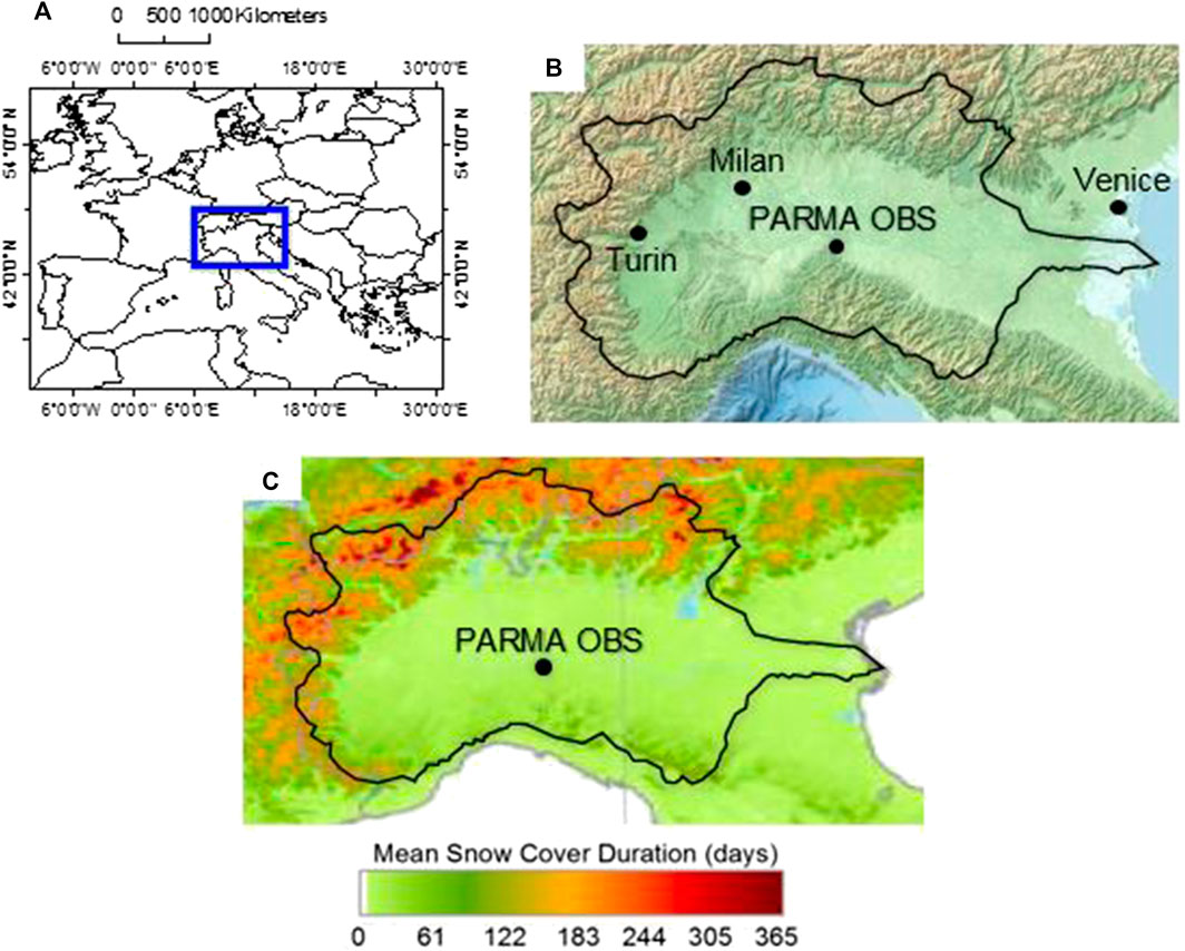
FIGURE 2. Geographical setting: (A) North Italy (blue square); (B) the Po River Basin (black curve) with main locations and Parma OBS; (C) related winter (November-March, 2000–2011) snow-cover duration. Maps are authors’ own elaboration from free, public domain images: (A) ESRI (http://www.esri.com) [Accessed September 10, 2020]; (B) Elastic Terrain Map (http://elasticterrain.xyz) [Accessed September 10, 2020]; (C)Dietz et al. (2012).
During the year, cyclonic Atlantic air masses and areas of anti-cyclonic airflows from central and eastern Europe alternate. Fields of variable winds are associated with wet air masses from southwest, and dry and continental winds from northeast. Snowfall increases with elevation until 2000 m a.s.l. Figure 3 (gray bars) refers to observed monthly snow cover days. At Parma OBS, which can be assumed sufficiently representative of the PRB area, the average of DSG in the period 1938–2018 is about 20 days year−1. Over this period of 81 years, the month of January had the greatest number of days with snow cover, with the soil covered by snow for about 10 days on average. On February, the number of days with snow on the ground roughly doubled the days of snow coverage in December. March and November had a similar number of days with snow cover, while the lowest number was registered in October. A similar distribution is noticeable for the 98th percentiles (Figure 3, empty bars).
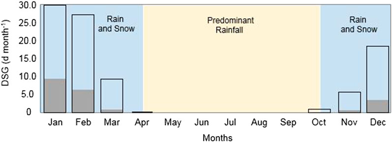
FIGURE 3. Monthly mean distribution of days of snow on the ground (DSG) at Parma OBS (gray bars) with the related 98th percentile (empty bars), calculated over the period 1938–2018.
The most abundant snowfall in the Alps and Apennines occurs during cold periods, in particular with the arrival of warmer and moist air from the south, with a rise in temperatures up to about 0°C. If plain areas are exposed to a degree of cold sufficiently intense, with temperature values below 0°C, snowfall and its persistence on the ground are also possible at very low altitudes (Bettini, 2016). This is what happens in the central-western sector of the PRB, when warm and humid air coming from the Mediterranean Sea slips on the cushion of cold air previously trapped in the low layers of mountain landscapes in the Alps and Apennines. There is a chance that the arrival of below-freezing temperatures can also bring snow along the PRB. In the presence of air masses close to saturation, very cold air suddenly entering the PRB raises near saturation leading wet air to condensation. This phenomenon, although rare, can be observed in the PRB when cold Siberian air penetrates westward into northern Italy, while very damp air or even a misty blanket stagnates in the plains. In these cases, snowfall is weak, of short duration and limited to the plains or the lowest slopes of the pre-Alps.
As covariates for the modeling of DSG, we referred to winter precipitation, and winter and spring air temperatures. Winter and spring are defined as periods from December to February, and from March to May, respectively. For the precipitation input, we used the seasonally-resolved data with 0.5° resolution, as arranged from Pauling et al. (2003). Likewise, we used seasonally-resolved winter and spring temperatures as arranged by Luterbacher et al. (2004) since 1500, and interpolated at the Parma OBS grid point. Both datasets were updated from the Climatic Research Unit global climate dataset (Jones and Harris, 2018). The database of observed DSG contains also the year 2019 (with 4 days of snow cover on the ground) but this year was left out of the analysis because the Climatic Research Unit data are updated until 2018 (checked on June 2020). For both winter precipitation and temperature, the analysis of the yearly data used (1681–2018 CE) shows that they are compliant with a normal distribution using the Kolmogorov-Smirnov test p > 0.05 (Supplementary Appendix A).
Development and Parameterization of the Statistical Model
The principle of parsimony as described in Mulligan and Wainwright (2013) states that a parsimonious model is the one with the greatest explanation or predictive power and least parameters or process complexity. Based on this principle, we developed a parsimonious model that could be easy parameterized and validated, and is reliable and applicable to the reconstruction of long-term historical DSG data. To increase predictability and minimize uncertainties in the modeling of annual DSG data, we built a nonlinear-multivariate regression with three input variables and three parameters considering the original observational 1938–2018 CE timeframe. The data resource of annual DSG data (81 years) was separated into two sub-sets to use roughly two-thirds (53 years) for calibration (1938–1990 CE) and one-third (28 years) for validation (1991–2018 CE). The calibration effort was thus anchored to the reality of snow-cover duration in the past to enable a reasonably accurate reconstruction of historical snow-cover days. A number of monthly climatic explanatory variables was considered during the input selection process. First, in order to reduce the number of inputs, we investigated the effects of single variables, or sets of variables, on DSG over some climatologically meaningful periods. Then, an iterative process (trial-and-error to decompose relevant drivers) enabled us to explain the dynamics of DSG in relatively simple terms. A stepwise selection logic was used to alternate between adding and removing terms. The following nonlinear multivariate regression model - DSG(Parma) - was thus derived to estimate DSG (day year−1) at Parma OBS:
where: A (day year−1) is a scale parameter corresponding to the number of DSG when the term between brackets is equal to unity; β (°C) and η are process parameters. Winter temperature, Tw (°C), is negatively related to DSG, as mediated by the shape in parameter η. Winter (w) and spring (s) temperature variability accounted for by the term VC is indicative of the instability of air masses near the Parma OBS. This approach discloses the association between the snowfall response variable DSG (Parma) and multiple predictors, such as the winter precipitation amount (P_w), winter mean air temperature (Tw), and winter-spring modified variation coefficient VC, that is, a standard deviation/mean ratio of winter and spring temperatures (T(w→s)), calculated across the current (t = 0) and previous (t = −1) years. This variability term is a key factor to infer inter-seasonal temperature fluctuations, as it is larger in the presence of snow.
The concept of the model (Figure 4) summarizes the mechanisms mostly driving the common patterns of change of snow-cover extent and duration (e.g., Brown et al., 2010; Brown, 2019). It shows that ∼10–15% of the Parma territory (central tendency) is covered by snow over wintertime. In this context, cool-season precipitation amounts are particularly important because the majority of annual precipitation occurs during the wintertime at medium-high latitudes, and preferentially as snow at high elevations through orographic enhancement (e.g., Dettinger et al., 1998; Selkowitz et al., 2002; Terzago et al., 2012; Luce et al., 2013). The logarithmic transformation of the total (solid and liquid) winter precipitation (ln(Pw)), which acts as snow-depth index in the model, was applied to underweight the amount of freshly fallen snow associated with broad-scale mixed precipitation over flat areas (e.g., Meir et al., 2016; Fehlmann et al., 2018). Snow-cover response to temperature includes the spatial extent (0.5°-grid resolution of winter temperatures) and the temporal scale (winter and spring months) over which the thermal forcing becomes important, by assuming that the object under study is a fractal (i.e., the site is a fractal element of the area). In this case, the scaling of the site can be reasonably modeled by a power-law process relationship, whose exponent η quantifies the spatial dependence (scaling nature) of the snow-cover days (Zhang et al., 2013). This is an issue of determining how the climate of a specific surface type differs from a grid-average climate, without formulating different model equations (Harvey, 2013). In particular, the η exponent does not only provide a parsimonious description of the process under study, but it is also a generic mechanism governing the process. In particular, higher exponent values obtained at a single site (compared to mean areal response) suggest that they can be regarded as a method to downscale areal (smoothed out) approximations to finer units (e.g., Spence and Mengistu, 2019).
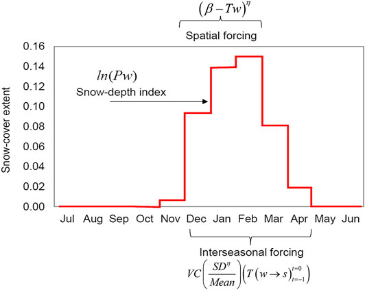
FIGURE 4. Monthly snow-cover extent in Parma territory (100-km square grid cell), with the associated driving factors. Monthly mean values (red line) were calculated on data provided for the period 1966–2018 by Global Snow Lab - Rutgers University Climate Lab (https://climate.rutgers.edu/snowcover) via KNMI-Climate Explorer Climate Change Atlas (http://climexp.knmi.nl) [Accessed September 10, 2020]. The three main terms of Eq. 1 are reported.
We have also found that a strong correlation (r = 0.84) exists between snowfall frequency and snow-cover duration at Parma in the period 1938–2018 CE (Supplementary Appendix B). However, since snowfall frequency measurements (i.e., snow days per year) only started in 1777 at Parma OBS, we excluded this input from the model, which was built on the temperature- and precipitation-based proxies allowing to extend the reconstruction period back to 1681. With this long-term series, we can detect patterns of climate change explaining fluctuations and tendencies in DSG data. Going back about 100 years before the beginning of the snowfall-frequency observations at Parma OBS, we could in fact start our DSG series at the turning point of the 17th and 18th centuries, at the so-called Maunder Minimum, which started in 1645 and lasted until 1715, a period characterized by exceedingly rare sunspots and lower-than-average temperatures (Eddy, 1976).
Spreadsheet-based model development and assessment were performed with the analytical and graphical support of STATGRAPHICS (Nau, 2005) and WESSA (Wessa, 2009) statistical software. The Mean Absolute Error (MAE, day year−1) was calculated to quantify the differences between actual and modeled DSG values, while the Kling-Gupta index (−∞<KGE ≤ 1; Kling et al., 2012) was used as efficiency measure (with KGE > –0.41 indicating that a model is better performing that the mean of observations as a benchmark predictor; Knoben et al., 2019). The Nash-Sutcliffe efficiency (−∞<EF ≤ 1, optimum; Nash and Sutcliffe, 1970) was also calculated as an uncertainty indicator of the model performance because greater values than 0.6 indicate limited model uncertainty, likely associated with narrow parameter uncertainty (Lim et al., 2006). With the determination coefficient (0 ≤ R2 ≤ 1, optimum), or the correlation coefficient (
Results and Discussion
Model Parameterization and Evaluation
For the reconstruction of a long-term annually-resolved DSG series, we first calibrated the DSG(Parma) model. The calibration work was performed through a trial-and-error process comparing the model estimates with observations until small MAE and large R2 values were obtained. Then, for the final selection of the parameter values, a third criterion (KGE closer to 1) was additionally involved. The calibrated parameters are: A = 0.0404 day year−1, β = 6.80°C, and η = 2.00. The value of the R2 statistic of observed (y) vs. modeled (x) data (Figure 5A) indicates that the fitted model explains 72% of the observed variability. The regression line y = 4.36 (±8.39) + 0.83 (±0.27)·x has intercept (a = 4.36) and slope (b = 0.83) with a relatively high standard error of the intercept (±8.39 days year−1) and a root mean standard error of the fit equals to 0.24 day year−1. This indicates the model’s lesser predictive ability for near-zero DSG, there is a superior predictive ability of Eq. 1 compared with a purely linear multivariate regression against the same independent variables, which produces several (unrealistic) negative values of DSG in both the calibration and validation periods (Supplementary Appendix C). The Nash-Sutcliffe efficiency value obtained in the calibration stage (EF = 0.73) indicates limited uncertainty in model estimates. Since the F-ratio p-value is less than 0.05, the linear regression between actual and estimated data is statistically significant. The mean absolute error (MAE), used to quantify the amount of error, was equal to 8.9 days year−1, which is lower than the standard error of the estimates (10.9 days year−1), while the Kling-Gupta index of 0.6 suggests a model of sufficient quality. The Durbin-Watson statistic (DW = 1.72, p = 0.14) reveals that there is no significant autocorrelation in the residuals.
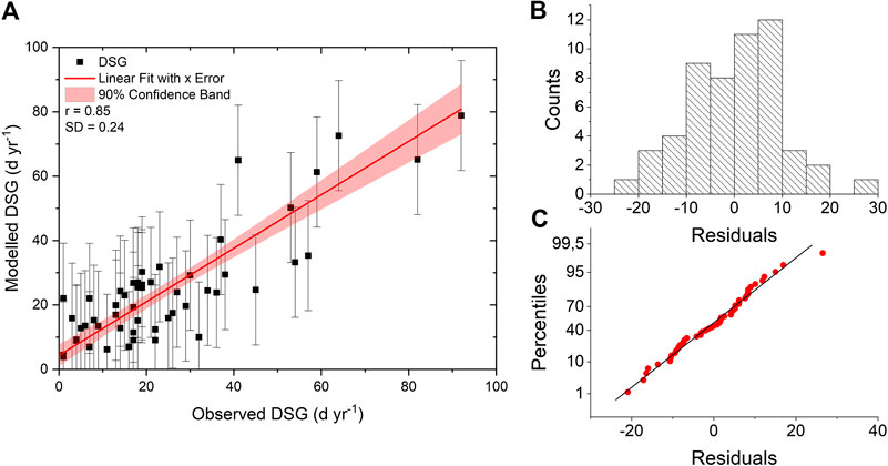
FIGURE 5. (A) Scatterplot of observed and modeled (Eq. 1) DSG at Parma OBS for the calibration sub-set (1938–1990), with regression line (red line), the bounds showing 90% confidence limits (pink colored band); (B) histogram of residuals; (C) Q-Q plot (sample vs. theoretical quantile values).
The model residuals approximate a normal distribution (Figure 5B; normality test, p > 0.05, Jarque and Bera, 1981) and the Q-Q plot (Figure 5C) exhibits a distribution of sample-quantiles around the theoretical line, indicating only a few biased high DSG values.
At the validation stage, the value of the R2 statistic indicates that 56% of the total variability in the observation is explained by the model, while MAE is equal to 4.4 days year−1, which is lower than the standard error of the estimates (5.7 days year−1), while the Kling-Gupta index is 0.6 (equal to the value obtained with the calibration set). Also in this case, the Durbin-Watson statistic (DW = 1.60, p = 0.13) indicates that there is no significant autocorrelation in the residuals. The timeline of DSG validation period shows the coevolution of observations and estimates (Figure 6A). The related distribution of model residuals (Figure 6A1) does not deviate significantly from normality (p > 0.05). In Figure 6B, the model estimates are compared to the decreasing trend (from 1950 to 2005) of the index obtained by De Bellis et al. (2010) for the Emilian Apennine, by averaging the snow-cover values of different mountain stations normalized with respect to the variability. We evaluated the relative performance of the DSG(Parma) model, without comparing the absolute estimates. Coevolution between the SCNI (snow-cover normalized index) and the modeled DSG illustrates a substantial agreement (r = 0.74).
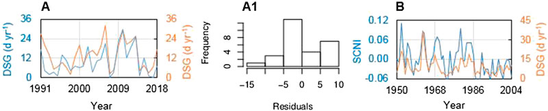
FIGURE 6. (A) Timeline evolution of observed (blue curve) and modeled (Eq. 1, orange curve) DSG for the validation sub-set (1991–2018); (A1) histogram of residuals; (B) timeline coevolution of observed Snow-Cover Normalized Index (SCNI) for the Emilian Apennine mountain range (blue curve) and modeled DSG at Parma OBS (orange curve) for the period 1950–2004.
We could get a slightly better performance by replacing Pw in Eq. 1 with the square root of snow days per year during both the calibration (R2 = 0.76, KGE = 0.81, MAE = 8.6 days year−1) and validation (R2 = 0.61, KGE = 0.52, MAE = 4.6 days year−1) periods. We concluded that this improvement is not such as to justify the limitation of the reconstruction to the SDY observation period alone (1777–2018). Equation 1 thus supports a broader reconstruction perspective. In determining whether the DSG (Parma) model can be simplified, we have fitted a multiple linear regression model to describe the relationship between DSG and the three independent variables Pw, Tw and VC in Eq. 1. The analysis of variance of the model gave p < 0.05 for each independent variable, the highest p-value being 0.04 for the term VC. This means that the model cannot be simplified further and its results correspond to criteria of stability, interpretability and usefulness (after Royston and Sauerbrei, 2008).
Time-Series Reconstruction of Snow-Cover Persistence on the Ground (1681–2018 CE)
Equation 1 was used to reconstruct the evolution of DSG over the period 1681–2018 CE (Figure 7A). The reconstructed time-series was then analyzed to find out possible climate patterns explaining variation in long-term trends of DSG, and to compare contemporary with historical DSG anomalies.
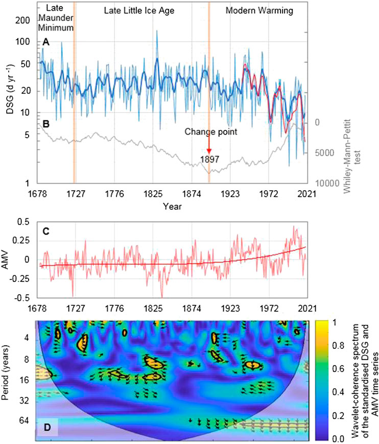
FIGURE 7. Overview of days with snow on the ground (DSG) patterns at Parma OBS along the period 1681–2018 CE: (A) Timeline evolution of DSG data reconstructed by Eq. 1 (light blue curve), with over-imposed 11-years Gaussian-filtered series for the whole period (bold blue curve) and the observational period 1938–2018 CE (red curve); (B) Mann-Whitney-Pettitt test statistic with the change point of 1897 (vertical red arrow); (C) time series of the Atlantic Multidecadal Variability (AMV; Wang et al., 2017) together with a polynomial (third-order) interpolation curve; (D) wavelet-coherence spectrum of the standardized DSG and AMV time series; bounded colors identify the 0.05 significance level areas; the bell-shaped, black contour marks the limit between the reliable region and the region below the contour where the edge effects occur (a.k.a. cone of influence); black arrows show the relative phase relationship, with in-phase pointing right, anti-phase pointing left, and AMV leading DSG by 90° pointing straight down.
Overall, the temporal evolution of annual values presents a downward trend (Mann-Kendall M-K trend test p < 0.01; Kendall, 1975), which appears more prominent in recent times (Figure 7A, blue curve and related Gaussian fitting; Figure 7B, Mann-Whitney-Pettitt statistic). We have used different statistical methods to identify distinct climatic patterns in the long-term DSG series. In fact, different test statistics are variously sensitive to change points located at the beginning, in the middle, or at the end of a time series (Martínez et al., 2009; Toreti et al., 2011), and a combination of statistical methods is considered to be most effective to track down change points (e.g., Wijngaard et al., 2003). The application of test statistics by Pettitt (1979) and Buishand (1982) suggests the existence of a change point in the year 1897. Since the late 19th century, the Atlantic Multidecadal Variability (AMV) has experienced a significant upward trend (Si et al., 2020), coinciding with the onset of the warming period (Figure 7C). Based on terrestrial proxy records from the circum-North Atlantic region, the AMV reconstruction by Wang et al. (2017) exhibits pronounced variability on multidecadal time-scales. This multi-decadal climate mode originates dynamically in the North Atlantic Ocean and propagates throughout the Northern Hemisphere via a suite of atmospheric and oceanic processes (Wyatt et al., 2012; Wang et al., 2018b). Sutton and Dong (2012) argued for the existence of a causal link between a positive phase of the AMV and drier conditions over the Mediterranean Basin. It is also known that winter precipitation in northern Italy is mainly caused by large-scale fronts of North Atlantic and Mediterranean synoptic low-pressure systems, which produce moderate but continuous precipitation (Hawcroft et al., 2012). Interannual to multi-decadal variability of this kind of precipitation is mainly modulated by the North Atlantic Oscillation (NAO; Pinto and Raible, 2012; Gómara et al., 2014; Gómara et al., 2016), describing the fluctuations in the difference of atmospheric pressure at sea level between the Icelandic Low and the Azores High.
Other test statistics detected a change point in 1830 (SNHT-double shift; Alexandersson and Moberg, 1997) or 1967 (Worsley likelihood; Worsley, 1986; penalized maximal t-test; Wang et al., 2007; SNHT-single series, Alexandersson, 1986), which merely support the idea of a long transition period going from the final phase of the Little Ice Age (LIA; ∼1300–1850 CE; Miller et al., 2012) to the most recent warming. These different statistically-relevant years provide a loose picture of climate-related DSG variations with changing climate patterns, where the cold conditions of the LIA are still dominating after the end of the Dalton minimum of reduced solar activity (∼1790–1830; Wagner and Zorita, 2005) until toward the end of the 19th century, but in the process of evolving into an incipient warming that becomes noticeable later in the 20th century (mostly by about 1960s). We refer hereafter to the year 1897 as a relevant change-point year, which is also the starting point of more erratic weather conditions. The long-term mean value of DSG (Table 1) is equal to 28 days year−1 (±16.8 days year−1 standard deviation) until the change-point year (Figure 7B) and to 21 days year−1 (±14.8 days year−1) after that point for the continuous predicted time series (Figure 7A, blue curve), while it is equal to 20 days year−1 (±11.9 days year−1) for the joined modeled and observed series (Figure 7A, joined blue and ochre curves after the year 1897).
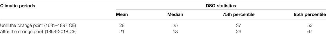
TABLE 1. Descriptive statistics of the DSG (days with snow on the ground, day year−1) time series for two climatic periods.
Considering that these two series, as well as the predicted and observed series for the period covered by observations (1938–2018 CE), are not statistically different (paired Student-t test, p-values >0.05), our analysis was based on the modeled values only. Table 1 also shows that the median and the 75th percentile values were higher over the period 1681–1897 CE, while more extreme values (95th percentile) were higher after the change point. The trend toward anomalously warm conditions over the 20th century and the beginning of the 21st century indicates that increasing temperatures represent the main factor triggering the decline of DSG, in particular over the most recent five decades where DSG have been subject to further decrease. This is in agreement with the contraction of snow-cover extent recently observed across Siberia and North America (e.g., Musselman et al., 2017; Zhang and Ma, 2018). It is striking that snow covered the ground over 145 days in the year 1830 and only over 99 days in the year 1709 (Figure 7A). The latter proved to be the coldest in memory, with a particularly long and hard freeze in a winter passed to the historical chronicles because of its cold and snowstorms. In the central Mediterranean, the severity of this winter was accompanied by ice and frozen water bodies like lakes and rivers (Glaser et al., 1994; Grove and Conterio, 1994), while snowfall continued from late December to mid-February, after which rain and snowmelt caused several rivers to overflow (Diodato et al., 2019). However, the 1829–1830 winter was not only described as harsh in all parts of Europe, but also early, with long and heavy snowfall from mid-November to the end of March (Corradi, 1865–1890, vol. III, p. 403). In January 1830, even the press was suspended because the roads, due to the abundance of snow, had not allowed the arrival of newspapers. The year 1830 was rather the end of a period that extended over important parts of the LIA, during which Europe experienced predominant cooling (Xoplaki et al., 2001). In fact, winter 1835–1836 was also remarkable for Milan and its region but not quite as severe as others (Stella, 1836, pp. 350–351):

The year 1684, at the beginning of our series, is also distinguished by a high number of days with snow on the ground (88 days). In this regard, Corradi Annals’ (1865–1890, vol. II, p. 257) define 1684 as the year in which snow covered the ground until after Easter:

After Xoplaki et al. (2001), the severe conditions during the winter 1683–1684 can be attributed to the presence of an extended high-pressure system over central and western Europe, with its center over north Iberia. This distribution of atmospheric pressure centers in Europe led to persistent northwesterly and/or northeasterly circulation over the Balkans and the eastern Mediterranean. These cold air outbreaks caused low or extremely low temperature conditions connected with precipitation events (rainfall and/or snowfall). Also noteworthy are the years 1947 and 1963, with snow on the ground over 79 and 73 days, respectively. January 1947 was recognized as historical for Italy, with very strong waves of frost and snow all over the country. The coldest winter in the post-World War II period was, however, 1962–1963: started on December, it continued with an escalation of continuous Siberian cold spell, alternating with Atlantic phases, until the month of March, which was equally rigid. In Britain, although the Thames had not frozen as in previous centuries, that winter turned out to be not only the coldest of the century but among the coldest ever. After that winter, the DSG median dropped further (only 15 days per year), and with it also the 95th percentile reached the lowest values ever (30 days per year). These trends are confirmed by the decrease in snow-cover extent in spring, as observed in Eurasia. Although the extent of the autumn snowpack has been limited in recent decades, and the winter trend has remained unchanged in Europe and Asia, a decrease in the snowpack extent and a greater variability in the transition seasons (spring and autumn) have been documented at the hemispheric scale since the 1920s (Krasting et al., 2013). Such snow-cover reduction was particularly significant in the mid-latitudes (40°–60°) of the Northern Hemisphere (Brown, 2000). Accordingly, Déry and Brown (2007) noted that the mean monthly snow-cover extent strongly anti-correlates with the mean air temperature in the Northern Hemisphere. This occurs particularly in April–June, when extended snow-cover duration is accompanied by intense incoming solar radiation.
We used the wavelet-coherence analysis for highlighting the time and frequency intervals when DSG and AMV have a significant interaction (Grinsted et al., 2004). The wavelet coherence method offers a bivariate extension of the wavelet analysis to identify regions with large common power in the time-frequency domain of the two time series, and reveals information about their phase relationship (which may be suggestive of dependency; Maraun and Kurths, 2004). The wavelet-coherence spectrum of the two time series (Figure 7D) displays sporadic high-frequency periodicities around 11 years. The quasi-11-year sunspot cycle is a main feature of solar activity (as identified by Wolf, 1852; Wolf, 1853). However, the 5% significance level is a not a reliable indication of dependency for erratic periods in the long-term behavior although Italian Alps snow-cover trends have been observed to oscillate with 11-year periods (Valt and Cianfarra, 2010). The region of the spectrum at lower-frequency periodicity of ∼60 years is quite extensive and suggestive of a causal AMV-DSG relationship emerging at the onset of the warm period (across the change-point year of 1897 with AMV leading in time), which appears to be linked to North Atlantic internal ocean-atmosphere variability (e.g., Knudsen et al., 2011; Mazzarella and Scafetta, 2012). However, the significant area falls outside of the cone of influence where edge effects become important and prevents this analysis from obtaining a robust interpretation in this sense.
Influence of Atmospheric Circulation Patterns of Snow-Cover Periods
The occurrence of snow events in Parma is to some extent related to the presence of a low-pressure system over the central Mediterranean area, which is a favourable configuration for several snow days and persistent snow. In order to discover if different climatic periods are somewhat the result of changes occurred in the continental atmospheric circulation, we created composite plots of sea-level pressure for the winters of the late Maunder Minimum (Figure 8A), the late LIA until the change-point year (Figure 8B) and the modern warming (Figure 8C). These climatic sub-periods reflect many dominant types of large-scale atmospheric circulation patterns, which are responsible for wintertime conditions over the Mediterranean region. During the first period, 1681–1715 (Figure 8A), the atmospheric pattern shows that the central Mediterranean area is characterized by a winter depression, which attracts cold arctic air masses from the north/northeast of Europe. In the period 1716–1897 (Figure 8B), a similar atmospheric circulation pattern continued to favor the transition of cold air masses from northern Europe though with a shallower depression center lessening snowfall and snow-cover duration. There were certainly less frequent and severe cold spells during the late LIA than in the Maunder Minimum. However, the late LIA was also characterized by some severe winters. To give an example, taken from Corradi (1865–1890, vol. II, p. 623), in 1782 the whole of Italy was besieged by a deadly bad weather:

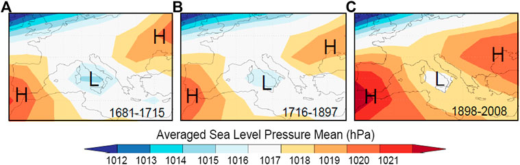
FIGURE 8. Mean reconstructed sea-level pressure (SLP) maps over southern Europe over the winters (December to March) of three periods: (A) late Maunder Minimum (1681–1715 CE); Late Little Ice Age (1716–1897 CE); (C) Modern Warming (1897–2008). L = low-pressure system (cyclone), H = high-pressure system (anticyclone). Maps are authors’ own elaboration using Climate Explorer (https://climexp.knmi.nl/start.cgi) [Accessed September 10, 2020] on data from: (A,B)Luterbacher et al. (2002); (C) from Küttel et al. (2010), which stops at year 2008.
The exit of the LIA generally offered less inclement winter weather. The map of the third period, 1898–2008 (Figure 8C), shows the squeezing and reabsorption of the depression center by two anticyclones, which is indicative of snow weather (both mean and extreme snowfall) becoming less common. The two high-pressure systems (Azores high to the west and Russian high to the east) prevented the Mediterranean from prolonged snow events of certain importance, as compared to the previous periods.
Conclusion
The annually-resolved DSG (days with snow on the ground) time-series reconstruction documents variations at Parma OBS since 1681. With this reconstruction, unprecedented in time length, we have deepened our understanding of the characteristics of snowfall in the Po valley (northern Italy) and reported the consistency of our model-based reconstruction of DSG with historical data. That consistency suggests that the reconstructed historical signal may be representative of real multi-decadal variations. In fact, our 339-year long time series of DSG shows a particularly marked downward trend in recent decades, after the change point detected in 1897, and suggests that important shifts in mean DSG values and their variability may be resolved by extended reconstruction. Interannual and inter-decadal variations are evident in the reconstruction. While the causes of the decrease observed in DSG are manifold and varied, two factors are recognisable: an increase in seasonal temperatures (Dobrovolný et al., 2010; Serquet et al., 2013) and a contraction in the variability of snow precipitations from 1 year to the next. With respect to the latter, we highlight a general shortening of snow duration due to a delay in the start date of snow cover in autumn and an advancement of the end date in spring, associated with a retreat of glaciers, mainly due to a decrease in winter precipitation (Vincent et al., 2005; Huss et al., 2008). However, other factors besides the increase in temperature may have caused a decrease in the snow-cover duration. Already in 1881, on the occasion of the royal meeting of the Accademia dei Lincei (“Lincean Academy”) in Rome (Italy), the Italian Catholic priest and geologist Antonio Stoppani (1824–1891) in a speech Sull’attuale regresso dei ghiacciai sulle Alpi (“On the current regression of glaciers in the Alps”) provided as a main cause of the regression of the glaciers, not the variations of temperature (even if they were of common knowledge), but the reduction of snowiness (e.g., Scaramellini and Bonardi, 2001). In fact, in that period the number of snow days had been reduced to roughly a third in just about 50 years, a worrying phenomenon, especially because at that time there were no dams and artificial reservoirs, and glaciers were among the few large reserves of water (e.g., Stoppani, 1876). Again, from 1797 to 1806 the days of snow in Milan (Italy) had been 243 (i.e., 26 on average per year), but the situation had substantially changed from 1857 to 1876 with 166 snow days (i.e., eight snow days per year). Recently, Diodato et al. (2020b) provided evidence for Switzerland that this decrease is continuing in the Alpine range.
In our study, we report the results without providing conclusive evidence regarding the causes of the observed changes in the reconstructed DSG. Our model results offer robustness against anthropogenic disturbance in urban environments. The latter is relevant for the Parma territory, where Zanella (1976) showed an average difference of 1.4°C between urban and rural temperature data in the period 1959–1973, and reported that the difference varied seasonally (especially in spring and summer). Heat islands may thus have been a contributing factor of the snow-cover decline (e.g., Musco, 2016) observed in this urban site (from about 80 days year−1 in the 1940s to <20 days year−1 in the most recent years), which appears to be sufficiently captured by the modeled time series. We have corroborated our findings suggesting that change points in snowfall series in northern Italy can be linked to large-scale changes in the modes of climate (e.g., the Atlantic Multidecadal Variability), identifying in this way the need for future research on the subject. Though the long-term trend of the DSG series may be represented by a combination of intermittent periodicities, due to the brevity of the time interval the presence of these periodicities and their relationship with snowfall mechanisms in northern Italy should be regarded as tentative, and in need of confirmation by additional studies on extended spatial scales.
Data Availability Statement
The raw data supporting the conclusions of this article will be made available by the authors, without undue reservation.
Author Contributions
ND conceived the study, performed the analysis and drafted the manuscript with GB, who wrote the final manuscript. CB prepared and organized the snowfall data used in the study, and contributed to scientific discussion of the article.
Conflict of Interest
The authors declare that the research was conducted in the absence of any commercial or financial relationships that could be construed as a potential conflict of interest.
Acknowledgments
We thank the NTNU publishing fund support to cover article-processing charges. The authors would like to thank Iñigo Gómara (Universidad Complutense de Madrid, Spain) for his support on wavelet-coherence analysis (wavelet software was provided by A. Grinsted).
Supplementary Material
The Supplementary Material for this article can be found online at: https://www.frontiersin.org/articles/10.3389/feart.2020.561148/full#supplementary-material
References
Adamson, G. C. D. (2015). Private diaries as information sources in climate research. WIREs Clim. Change. 6, 599–611. doi: 10.1002/wcc.365
Alexandersson, H. (1986). A homogeneity test applied to precipitation data. J. Climatol. 6, 661–675. doi: 10.1002/joc.3370060607
Alexandersson, H., and Moberg, A. (1997). Homogenization of Swedish temperature data. Part I: homogeneity test for linear trends. Int. J. Climatol. 17, 25–34. doi: 10.1002/(sici)1097-0088(199701)17:1<25::aid-joc103>3.0.co;2-j
Barnhart, T. B., Molotch, N. P., Livneh, B., Harpold, A. A., Knowles, J. F., and Schneider, D. (2016). Snowmelt rate dictates streamflow. Geophys. Res. Lett. 43, 8006–8016. doi: 10.1002/2016GL069690
Bednorz, E. (2004). Snow cover in eastern Europe in relation to temperature, precipitation and circulation. Int. J. Climatol. 24, 591–601. doi: 10.1002/joc.1014
Bettini, E. (2016). Climatologica dinamica delle precipitazioni sulla località di Milano. Environmental and Land Planning Engineering Msthesis. Milan (Italy): Polytechnic University of Milan [in Italian].
Bradley, R. S., and Jones, P. D. (1992). “Records of explosive volcanic eruptions over the last 500 years,” in Climate since A.D. 1500. Editors R. S. Bradley, and P. D. Jones, (London, UK: Routledge), 606–622.
Brázdil, R., Pfister, C., Wanner, H., Von Storch, H., and Luterbacher, J. (2005). Historical climatology in Europe - the state of the art. Clim. Change. 70, 363–430. doi: 10.1007/s10584-005-5924-1
Brown, I. (2019). Snow cover duration and extent for Great Britain in a changing climate: altitudinal variations and synoptic‐scale influences. Int. J. Climatol. 39, 4611–4626. doi: 10.1002/joc.6090
Brown, R. D. (2000). Northern Hemisphere snow cover variability and change, 1915–97. J. Climate. 13, 2339–2355. doi: 10.1175/1520-0442(2000)013<2339:NHSCVA>2.0.CO;2
Brown, R., Derksen, C., and Wang, L. (2010). A multi-data set analysis of variability and change in Arctic spring snow cover extent, 1967-2008. J. Geophys. Res. 115, D16111. doi: 10.1029/2010JD013975
Buishand, T. A. (1982). Some methods for testing the homogeneity of rainfall records. J. Hydrol. 58, 11–27. doi: 10.1016/0022-1694(82)90066-X
Camuffo, D., and Bertolin, C. (2012). The earliest temperature observations in the world: the Medici Network (1654-1670). Clim. Change. 111, 335–363. doi: 10.1007/s10584-011-0142-5
Changnon, S. A., and Changnon, D. (2006). A spatial and temporal analysis of damaging snowstorms in the United States. Nat. Hazards 37 (3), 373–389.
Clark, M. P., Serreze, M. C., and Robinson, D. A. (1999). Atmospheric controls on Eurasian snow extent. Int. J. Climatol. 19, 27–40. doi: 10.1002/(SICI)1097-0088(199901)19:1<27::AID-JOC346>3.0.CO;2-N
Cohen, J., and Rind, D. (1991). The effect of snow cover on the climate. J. Climate. 4, 689–706. doi: 10.1175/1520-0442(1991)004<0689:TEOSCO>2.0.CO;2
Colla, A. (1840). Giornale Meteorologico dell’anno 1839. Parma: registro manoscritto delle osservazioni fatte nella specola dell’Università. Parma: University of Parma [in Italian].
Corradi, A. (1865–1890). Annali delle epidemie occorse in Italia dalle prime memorie fino al 1850. Bologna, Italy: Arnaldo Forni, Vol. 5 (reprint in 1972). [in Italian].
Croce, P., Formichi, P., Landi, F., Mercogliano, P., Bucchignani, E., Dosio, A., et al. (2018). The snow load in Europe and the climate change. Clim. Risk Manage. 20, 138–154. doi: 10.1016/j.crm.2018.03.001
Davi, N. K., Jacoby, G. C., D'Arrigo, R. D., Baatarbileg, N., Jinbao, L., and Curtis, A. E. (2012). A tree-ring-based drought index reconstruction for far-western Mongolia: 1565-2004. Int. J. Climatol. 29, 1508–1514.
De Bellis, A., Pavan, V., and Levizzani, V. (2010). Bologna: Technical Report ARPA-SIMC – 19. Climatologia e variabilità interannuale della neve sull’Appennino Emiliano-Romagnolo. Available at: https://www.arpae.it/cms3/documenti/_cerca_doc/meteo/quaderni/quaderno_neve_2010.pdf (Accessed September 10, 2020).
De Walle, D., and Rango, A. (2008). Principles of snow hydrology. Cambridge, UK: Cambridge University Press. doi: 10.1017/CBO9780511535673
Déry, S. J., and Brown, R. D. (2007). Recent Northern Hemisphere snow cover extent trends and implications for the snow-albedo feedback. Geophys. Res. Lett. 34, L22504. doi: 10.1029/2007GL031474
Dettinger, M. D., Cayan, D. R., Diaz, H. F., and Meko, D. M. (1998). North‐South precipitation patterns in western North America on interannual‐to‐decadal timescales. J. Clim. 11, 3095–3111. doi: 10.1175/1520‐0442(1998)011<3095:NSPPI10.1175/1520-0442(1998)011<3095:nsppiw>2.0.co;2
Dietz, A. J., Wohner, C., and Kuenzer, C. (2012). European snow cover characteristics between 2000 and 2011 derived from improved modis daily snow cover products. Rem. Sens. 4, 2432–2454. doi: 10.3390/rs4082432
Diodato, N. (1997). Paesaggi d’inverno: aspetti naturalistici e climatologici delle nevicate sulla Campania interna. Benevento: La Provincia Sannita. 17 [in Italian].
Diodato, N., and Bellocchi, G. (2020). Climate control on snowfall days in peninsular Italy. Theor. Appl. Climatol. 140, 951–961. doi: 10.1007/s00704-020-03136-0
Diodato, N., Büntgen, U., and Bellocchi, G. (2019). Mediterranean winter snowfall variability over the past Millennium. Int. J. Climatol. 39, 384–394. doi: 10.1002/joc.5814
Diodato, N., Bertolin, C., Bellocchi, G., Ferri, L., and Fantini, P. (2020a). New insights into the world’s longest series of monthly snowfall (Parma, Northern Italy, 1777‐2018). Int. J. Climatol. 6766, 1–17 [accepted]. doi: 10.1002/joc.6766
Diodato, N., Fratianni, S., and Bellocchi, G. (2020b). Reconstruction of snow days based on monthly climate indicators in the Swiss pre-alpine region. Reg. Environ. Change. 20, 55. doi: 10.1007/s10113-020-01639-0
Dobrovolný, P., Moberg, A., Brázdil, R., Pfister, C., Glaser, R., Wilson, R., et al. (2010). Monthly, seasonal and annual temperature reconstructions for Central Europe derived from documentary evidence and instrumental records since AD 1500. Clim. Change. 101, 69–107. doi: 10.1007/s10584-009-9724-x
Durbin, J., and Watson, G. S. (1950). Testing for serial correlation in least squares regression. I. Biometrika 37 (3–4), 409–428. doi: 10.1093/biomet/37.3-4.409. JSTOR 2332391
Durbin, J., and Watson, G. S. (1951). Testing for serial correlation in least squares regression. II. Biometrika 38 (1–2), 159–179. doi: 10.1093/biomet/38.1-2.159. JSTOR 2332325
Eddy, J. A. (1976). The maunder minimum. Science. 192, 1189–1202. doi: 10.1126/science.192.4245.118910.1126/science.192.4245.1189
Enzi, S., Bertolin, C., and Diodato, N. (2014). Snowfall time-series reconstruction in Italy over the last 300 years. Holocene. 24, 346–356. doi: 10.1177/0959683613518590
Falarz, M. (2004). Variability and trends in the duration and depth of snow cover in Poland in the 20th century. Int. J. Climatol. 24, 1713–1727. doi: 10.1002/joc.1093
Fehlmann, M., Gascón, E., Rohrer, M., Schwarb, M., and Stoffel, M. (2018). Estimating the snowfall limit in alpine and pre-alpine valleys: a local evaluation of operational approaches. Atmos. Res. 204, 136–148. doi: 10.1016/j.atmosres.2018.01.016
Glaser, R., and Riemann, D. (2009). A thousand-year record of temperature variations for Germany and Central Europe based on documentary data. J. Quat. Sci. 24, 437–449. doi: 10.1002/jqs.1302
Glaser, R., Militzer, S., and Busche, D. (1994). “A contribution to the reconstruction of climate in Germany during the Late Maunder Minimum (1675 to 1715),” in Climatic trends and anomalies in Europe 1675–1715. Editors B. Frenzel, C. Pfister, and B. Gläser, (Stuttgart, Germany: Gustav Fischer), 173–190.
Godsey, S. E., Kirchner, J. W., and Tague, C. L. (2014). Effects of changes in winter snowpacks on summer low flows: case studies in the Sierra Nevada, California, USA. Hydrol. Process. 28, 5048–5064. doi: 10.1002/hyp.9943
Gómara, I., Rodríguez-Fonseca, B., Zurita-Gotor, P., and Pinto, J. G. (2014). On the relation between explosive cyclones affecting Europe and the North Atlantic Oscillation. Geophys. Res. Lett. 41, 2182–2190. doi: 10.1002/2014GL059647
Gómara, I., Rodríguez-Fonseca, B., Zurita-Gotor, P., Ulbrich, S., and Pinto, J. G. (2016). Abrupt transitions in the NAO control of explosive North Atlantic cyclone development. Clim. Dynam. 47, 3091–3111. doi: 10.1007/s00382-016-3015-9
Goward, S. N. (2005). “Albedo and reflectivity,” in Encyclopedia of world climatology. Editor J. E. Oliver, (Dordrecht, Neitherlands: encyclopedia of earth sciences series., Springer), 32–35.
Granger, C. W. J., Hyung, N., and Jeon, Y. (2001). Spurious regressions with stationary series. Appl. Econ, 33 (7), 899–904.
Grinsted, A., Moore, J. C., and Jevrejeva, S. (2004). Application of the cross wavelet transform and wavelet coherence to geophysical time series. Nonlinear Process. Geophys. 11, 561–566. doi: 10.5194/npg-11-561-2004
Grove, J. M., and Conterio, A. L. (1994). “Climate in the eastern mediterranean, 1675 to 1715,” in Climatic trends and anomalies in Europe 1675-1715. Editors B. Frenzel, C. Pfister, and B. Gläser, (Stuttgart, Germany: Gustav Fischer), 275–285.
Handmer, J., Honda, Y., Kundzewicz, Z., Arnell, N., Benito, G., Hatfield, J., et al. (2012). “Changes in impacts of climate extremes: human systems and ecosystems,” in Managing the Risks of Extreme Events and Disasters to Advance Climate Change Adaptation: Special Report of the Intergovernmental Panel on Climate Change. Editors C. Field, V. Barros, T. Stocker, and Q. Dahe (Cambridge: Cambridge University Press),. 231–290. doi: 10.1017/CBO9781139177245.007
Harvey, L. D. D. (2013). “Climate and climate-system modelling,” in Environmental modelling: finding simplicity in complexity. Editors J. Wainwright, and M. Mulligan, (Chichester, UK: John Wiley & Sons), 151–164.
Hawcroft, M. K., Shaffrey, L. C., Hodges, K. I., and Dacre, H. F. (2012). How much Northern Hemisphere precipitation is associated with extratropical cyclones? Geophys. Res. Lett. 39, L24809. doi: 10.1029/2012GL053866
Huss, M., Bauder, A., Funk, M., and Hock, R. (2008). Determination of the seasonal mass balance of four Alpine glaciers since 1865. J. Geophys. Res. 113, F01015. doi: 10.1029/2007JF000803
Jarque, C. M., and Bera, A. K. (1981). An efficient large-sample test for normality of observations and regression residuals. Working Papers in Economics and Econometrics 40. Canberra, Australia: The Australian National University.
Jennings, K. S., Winchell, T. S., Livneh, B., and Molotch, N. P. (2018). Spatial variation of the rain-snow temperature threshold across the Northern Hemisphere. Nat. Commun. 9, 1148. doi: 10.1038/s41467-018-03629-7
Jones, P. D., and Harris, I. C. (2018). Climatic Research Unit (CRU): time-series (TS) datasets of variations in climate with variations in other phenomena v3. Leeds: NCAS British Atmospheric Data CentreAvailable at: http://catalogue.ceda.ac.uk/uuid/3f8944800cc48e1cbc29a5ee12d8542d (Accessed September 10, 2020). doi: 10.4324/9781315268590
Knudsen, M. F., Seidenkrantz, M.-S., Jacobsen, B. H., and Kuijpers, A. (2011). Tracking the atlantic multidecadal oscillation through the last 8,000 years. Nat. Commun. 2, 178. doi: 10.1038/ncomms1186
Knoben, W. J. M., Freer, J. E., and Woods, R. A. (2019). Inherent benchmark or not? Comparing Nash-Sutcliffe and Kling-Gupta efficiency scores. Hydrol. Earth Syst. Sci. 23 (10), 4323–4331.
Kling, H., Fuchs, M., and Paulin, M. (2012). Runoff conditions in the upper Danube basin under an ensemble of climate change scenarios. J. Hydrol. 424–425, 264–277. doi: 10.1016/j.jhydrol.2012.01.011
Krasting, J. P., Broccoli, A. J., Dixon, K. W., and Lanzante, J. R. (2013). Future changes in Northern Hemisphere snowfall. J. Clim. 26, 7813–7828. doi: 10.1175/JCLI-D-12-00832.1
Kretschmer, M., Cohen, J., Matthias, V., Runge, J., and Coumou, D. (2018). The different stratospheric influence on cold-extremes in Eurasia and North America. NPJ Clim. Atmos. Sci. 1, 44. doi: 10.1038/s41612-018-0054-4
Kunkel, K. E., Robinson, D. A., Champion, S., Yin, X., Estilow, T., and Frankson, R. M. (2016). Trends and extremes in Northern Hemisphere snow characteristics. Curr. Clim. Change Rep. 2, 65–73. doi: 10.1007/s40641-016-0036-8
Küttel, M., Xoplaki, E., Gallego, D., Luterbacher, J., García-Herrera, R., Allan, R., et al. (2010). The importance of ship log data: reconstructing North Atlantic, European and Mediterranean sea level pressure fields back to 1750. Clim. Dynam. 34, 1115–1128. doi: 10.1007/s00382-009-0577-9
Leporati, E., and Mercalli, L. (1994). Snowfall series of Turin, 1784-1992: climatological analysis and action on structures. Ann. Glaciol. 19, 77–84. doi: 10.3189/S0260305500011010
Lim, K. J., Engel, B. A., Tang, Z., Muthukrishnan, S., Choi, J., and Kim, K. (2006). Effects of calibration on L-THIA GIS runoff and pollutant estimation. J. Environ. Manag. 78, 35–43. doi: 10.1016/j.jenvman.2005.03.014
Luce, C. H., Abatzoglou, J. T., and Holden, Z. A. (2013). The missing mountain water: slower westerlies decrease orographic enhancement in the Pacific Northwest USA. Science. 342, 1360–1364. doi: 10.1126/science.1242335
Lute, A. C., Abatzoglou, J. T., and Hegewisch, K. C. (2015). Projected changes in snowfall extremes and interannual variability of snowfall in the Western United States. Water Resour. Res. 51, 960–972. doi: 10.1002/2014WR016267
Luterbacher, J., Xoplaki, E., Dietrich, D., Rickli, R., Jacobeit, J., Beck, C., et al. (2002). Reconstruction of sea level pressure fields over the eastern North Atlantic and Europe back to 1500. Clim. Dynam. 18, 545–561. doi: 10.1007/s00382-001-0196-6
Luterbacher, J., Dietrich, D., Xoplaki, E., Grosjean, M., and Wanner, H. (2004). European seasonal and annual temperature variability, trends, and extremes since 1500. Science. 303, 1499–1503. doi: 10.1126/science.1093877
Mangianti, F., and Beltrano, M. C. (1993). La neve a Roma dal 1741 al 1990. Roma: Central Office of Agricultural Ecology of the Italian Ministry of Agriculture. [in Italian].
Mann, M. E., Gille, E., Bradley, R. S., Hughes, M. K., Overpeck, J., Keimig, F. T., et al. (2000). Global temperature patterns in past centuries: an interactive presentation. Earth Interact. 4, 1–29. doi: 10.1175/1087-3562(2000)004<0001:GTPIPC>2.3.CO;2
Maraun, D., and Kurths, J. (2004). Cross wavelet analysis: significance testing and pitfalls. Nonlinear Process. Geophys. 11, 505–514. doi: 10.5194/npg-11-505-2004
Martínez, M. D., Serra, C., Burgueño, A., and Lana, X. (2009). Time trends of daily maximum and minimum temperatures in Catalonia (ne Spain) for the period 1975-2004. Int. J. Climatol. 30, 267–290. doi: 10.1002/joc.1884
Mazzarella, A., and Scafetta, N. (2012). Evidences for a quasi 60-year North Atlantic Oscillation since 1700 and its meaning for global climate change. Theor. Appl. Climatol. 107, 599–609. doi: 10.1007/s00704-011-0499-4
Meir, P., Cox, P., and Grace, J. (2006). The influence of terrestrial ecosystems on climate. Trends Ecol. Evol. 21, 254–260.
Miller, G. H., Geirsdóttir, Á., Zhong, Y., Larsen, D. J., Otto-Bliesner, B. L., Holland, M. M., et al. (2012). Abrupt onset of the Little Ice Age triggered by volcanism and sustained by sea-ice/ocean feedbacks. Geophys. Res. Lett. 39, L02708. doi: 10.1029/2011GL050168
Mulligan, M., and Wainwright, J. (2013). “Modelling and model building,” in Environmental modelling: finding simplicity in complexity. Editors J. Wainwright, and M. Mulligan, (Chichester: John Wiley & Sons), 5–29.
Musco, F. (2016). Counteracting Urban Heat Island Effects in a Global Climate Change Scenario. Switzerland: Springer International Publishing AG.
Musselman, K. N., Clark, M. P., Liu, C., Ikeda, K., and Rasmussen, R. (2017). Slower snowmelt in a warmer world. Nat. Clim. Change. 7, 214–219. doi: 10.1038/nclimate3225
Nash, J. E., and Sutcliffe, J. V. (1970). River flow forecasting through conceptual models part I - a discussion of principles. J. Hydrol. 10, 282–290. doi: 10.1016/0022-1694(70)90255-6
Nau, R. (2005). STATGRAPHICS V.5: Overview & tutorial guide, http://www.duke.edu/∼rnau/sgwin5.pdf.
O'Gorman, E. J. (2014). Integrating comparative functional response experiments into global change research. J. Anim. Ecol. 83 (3), 525–527.
Pauling, A., Luterbacher, J., and Wanner, H. (2003). Evaluation of proxies for European and North Atlantic temperature field reconstructions. Geophys. Res. Lett. 30, 1787. doi: 10.1029/2003GL017589
Petkova, N., Koleva, E., and Alexandrov, V. (2004). Snow cover variability and change in mountainous regions of Bulgaria, 19312000. Meteorol. Z. 13, 19–23. doi: 10.1127/0941-2948/2004/0013-0019
Pettitt, A. N. (1979). A non-parametric approach to the change-point problem. Appl. Stat. 28, 126–135. doi: 10.2307/2346729
Pimentel, R., Herrero, J., and Polo, M. (2017). Quantifying snow cover distribution in semiarid regions combining satellite and terrestrial imagery. Rem. Sens. 9, 995. doi: 10.3390/rs9100995
Pinto, J. G., and Raible, C. C. (2012). Past and recent changes in the North Atlantic oscillation. WIREs Clim. Change, 7, 79–90. doi: 10.1002/wcc.150
Sandells, M., and Flocco, D. (2014). “Snow,” in Introduction to the physics of the cryosphere. Editors M. Sandells, and D. Flocco, (Reading, UK: Morgan & Claypool Publishers), Vol. 3, 3.1–3.17.
Scaramellini, G., and Bonardi, L. (2001). La géographie italienne et les Alpes de la fin du XIXe siècle à la Seconde Guerre mondiale. Revue de Géographie Alpine. 89, 133–158. [in French]. doi: 10.3406/rga.2001.3062
Selkowitz, D. J., Fagre, D. B., and Reardon, B. A. (2002). Interannual variations in snowpack in the crown of the continent ecosystem. Hydrol. Process. 16, 3651–3665. doi: 10.1002/hyp.1234
Serquet, G., Marty, C., and Rebetez, M. (2013). Monthly trends and the corresponding altitudinal shift in the snowfall/precipitation day ratio. Theor. Appl. Climatol. 114, 437–444. doi: 10.1007/s00704-013-0847-7
Si, D., Jiang, D., and Wang, H. (2020). Intensification of the atlantic multidecadal variability since 1870: implications and possible causes. J. Geophys. Res. Atmos. 125, e2019JD030977. doi: 10.1029/2019JD030977
Spence, C., and Mengistu, S. G. (2019). On the relationship between flood and contributing area. Hydrol. Process. 33, 1980–1992. doi: 10.1002/hyp.13467
Stella, A. F. (1836). Biblioteca italiana ossia giornale di letteratura scienze ed arti compilato da una societa di letterati. Tomo, LXXXI. Milano, Italy: Direzione del Giornale di Letteratura, Scienze ed Arti [in Italian].
Stoppani, A. (1876). Il Bel Paese. Conversazioni sulle bellezze naturali, la geologia, e la geografia fisica d'Italia. Milan: Tipografia e Libreria Editrice Ditta Giacomo Agnelli. [in Italian].
Sutton, R. T., and Dong, B. (2012). Atlantic Ocean influence on a shift in European climate in the 1990s. Nat. Geosci. 5, 788–792. doi: 10.1038/ngeo1595
Terzago, S., Fratianni, S., and Cremonini, R. (2012). Winter precipitation in Western Italian Alps (1926-2010). Meteorol. Atmos. Phys. 119, 125–136. doi: 10.1007/s00703-012-0231-7
Toreti, A., Kuglitsch, F. G., Xoplaki, E., Della-Marta, P. M., Aguilar, E., Prohom, M., et al. (2011). A note on the use of the standard normal homogeneity test to detect inhomogeneities in climatic time series. Int. J. Climatol. 31, 630–632. doi: 10.1002/joc.2088
UNESCO/IASH/WMO (1970). Seasonal snow cover. Paris: United Nations Educational, Scientific and Cultural Organization.
Valt, M., and Cianfarra, P. (2010). Recent snow cover variability in the Italian Alps. Cold Reg. Sci. Technol. 64, 146–157. doi: 10.1016/j.coldregions.2010.08.008
Vincent, C., Le Meur, E., and Six, D. (2005). Solving the paradox of the end of the Little Ice Age in the Alps. Geophys. Res. Lett. 32, L09706. doi: 10.1029/2005GL022552
Wagner, S., and Zorita, E. (2005). The influence of volcanic, solar and CO2 forcing on the temperatures in the Dalton Minimum (1790-1830): a model study. Clim. Dynam. 25, 205–218. doi: 10.1007/s00382-005-0029-0
Wang, J., Liang, Z., Wang, D., Liu, T., and Yang, J. (2016). Impact of climate change on hydrologic extremes in the Upper Basin of the Yellow River Basin of China. Adv. Meteorol. 2016, 1–13. doi: 10.1155/2016/1404290
Wang, J., Yang, B., Ljungqvist, F. C., Luterbacher, J., Osborn, T. J., Briffa, K. R., et al. (2017). Internal and external forcing of multidecadal Atlantic climate variability over the past 1,200 years. Nat. Geosci. 10, 512–517. doi: 10.1038/ngeo2962
Wang, X. L., Wen, Q. H., and Wu, Y. (2007). Penalized maximal t test for detecting undocumented mean change in climate data series. J. Appl. Meteorolog. Clim. 46, 916–931. doi: 10.1175/JAM2504.1
Wang, Y., Yang, J., Chen, Y., Wang, A., and De Maeyer, P. (2018a). The spatiotemporal response of soil moisture to precipitation and temperature changes in an arid region, China. Rem. Sens. 10, 468. doi: 10.3390/rs10030468.
Wang, Y., Yang, B., Osborn, T. J., Ljungqvist, F. C., Zhang, H., and Luterbacher, J. (2018b). Causes of East Asian temperature multidecadal variability since 850 CE. Geophys. Res. Lett. 45, 13485–13494. doi: 10.1029/2018GL080725
Wessa, P. (2012). Free statistics software, version 1.1.23-r7. Office for Research Development and Education, http://www.wessa.net.
Wijngaard, J. B., Klein Tank, A. M. G., and Können, G. P. (2003). Homogeneity of 20th century European daily temperature and precipitation series. Int. J. Climatol. 23, 679–692. doi: 10.1002/joc.906
WMO (2008). Annual bulletin on the climate in WMO region VI - Europe and Middle East - 2008. Offenbach am Main: Deutscher Wetterdienst.
Wolf, R. (1852). Neue Untersuchungen über die Periode der Sonnenflecken und ihre Bedeutung. Mitt. Naturforsch. Ges. Bern. 255, 249–270. [in German].
Wolf, R. (1853). Ueber den Zusammenhang magnetischer Erscheinungen mit dem Zustande der Sonne. Astr. Nachr. AN. 35, 59–60. [in German]. doi: 10.1002/asna.18530350407
Worsley, K. J. (1986). Confidence regions and tests for a change-point in a sequence of exponential family random variables. Biometrika. 73, 91–104. doi: 10.1093/biomet/73.1.91
Wyatt, M. G., Kravtsov, S., and Tsonis, A. A. (2012). Atlantic multidecadal oscillation and Northern Hemisphere’s climate variability. Clim. Dynam. 38, 929–949. doi: 10.1007/s00382-011-1071-8
Xoplaki, E., Maheras, P., and Luterbacher, J. (2001). Variability of climate in Meridional Balkans during the periods 1675-1715 and 1780-1830 and its impact on human life. Clim. Change. 48, 581–615. doi: 10.1023/A:1005616424463
Yarnell, S. M., Viers, J. H., and Mount, J. F. (2010). Ecology and management of the spring snowmelt recession. Bioscience. 60, 114–127. doi: 10.1525/bio.2010.60.2.6
Zhang, X., Drake, N. A., and Wainwright, J. (2013). “Spatial modelling and scaling issues,” in Environmental modelling: finding simplicity in complexity. Editors J. Wainwright, and M. Mulligan, (Chichester: John Wiley & Sons), 69–90.
Keywords: snow cover, snow on the ground, negative trend, Southern Europe, Parma, multi-centennial, reconstruction, historical dataset
Citation: Diodato N, Bertolin C and Bellocchi G (2020) Multi-Decadal Variability in the Snow-Cover Reconstruction at Parma Observatory (Northern Italy, 1681–2018 CE). Front. Earth Sci. 8:561148. doi: 10.3389/feart.2020.561148
Received: 11 May 2020; Accepted: 22 September 2020;
Published: 30 October 2020.
Edited by:
Reik Donner, Hochschule Magdeburg-Stendal, GermanyReviewed by:
Jiri Miksovsky, Charles University, CzechiaDörthe Handorf, Alfred Wegener Institute Helmholtz Centre for Polar and Marine Research (AWI), Germany
Copyright © 2020 Diodato, Bertolin and Bellocchi. This is an open-access article distributed under the terms of the Creative Commons Attribution License (CC BY). The use, distribution or reproduction in other forums is permitted, provided the original author(s) and the copyright owner(s) are credited and that the original publication in this journal is cited, in accordance with accepted academic practice. No use, distribution or reproduction is permitted which does not comply with these terms.
*Correspondence: Chiara Bertolin, Y2hpYXJhLmJlcnRvbGluQG50bnUubm8=