 Hongwei Wang1,2
 Ruizhi Wen1,2*
- 1Institute of Engineering Mechanics, China Earthquake Administration, Harbin, China
- 2Key Laboratory of Earthquake Engineering and Engineering Vibration of China Earthquake Administration, Harbin, China
We separated the propagation path attenuation and source spectra from the S-wave Fourier amplitude spectra of the observed ground motions recorded during 46 small-to-moderate earthquakes in the junction of the northwest Tarim Basin and Kepingtage fold-and-thrust zone, mainly composed of two Jiashi seismic sequences in 2020 and 2018. Slow seismic wave decay was observed as the distance increased, while the quality factor regressed as 60.066 f0.988 for frequency f = 0.254–30 Hz reflects the strong anelastic attenuation in the study region. We estimated the stress drops for the 46 earthquakes under investigation from the preferred corner frequencies and seismic moments by fitting the inverted source spectra and the theoretical ω-square model. The relationship between seismic moment and corner frequency and the dependence of the stress drop on the moment magnitude reveal the breakdown of earthquake self-similar scaling for the events in this study. The temporal variation in stress drops indicates that the mainshock plays a short-term role in the source characteristics of the surrounding earthquakes. Aftershocks immediately following the mainshock show a low stress release and then gradually recover in a short time. The healing process for the fractured fault in the mainshock may be one reason for the stress drop recovery of the aftershock. The foreshock with the low stress release occurring in the high-heterogeneity fault zone may motivate the following occurrence of the largest magnitude mainshock with a high stress drop. We inferred that the foreshock-mainshock behavior, including several moderate events, may be predisposed to occur in our study region characterized by an inhomogeneous crust.
Introduction
A moderate earthquake of Ms 5.4 abruptly shook the Jiashi county of the Xinjiang region in northwest China on January 18, 2020, at 00:05 Beijing time (Figure 1), arousing the 2020 Jiashi seismic sequence. This sequence rapidly reached its climax on the following night as the largest magnitude mainshock, measured as Ms 6.4, occurred ∼2.5 km to the east of the Ms 5.4 foreshock, and a great number of aftershocks followed immediately, including the largest one measured as Ms 5.2 about 22 km to the east of the mainshock. However, the Ms 5.4 foreshock and Ms 6.4 mainshock did not share similar rupture mechanisms according to the fault plane solutions reported by the United States Geology Survey, strike slip for the former, and low-angle reverse dip slip for the latter (Figure 1). On February 21, 2020, another moderate earthquake of Ms 5.1 adjacent to the Ms 5.2 largest aftershock occurred at the easternmost end of this sequence (Figure 1). Up until March 1, 2020, this sequence consisted of 26 events of Ms ≥ 3.0 [derived from China Earthquake Network Center (CENC), www.ceic.ac.cn/history], primarily assembled in a narrow belt in a nearly east-west orientation and nucleated in the upper crust mostly at a depth of 15–20 km.
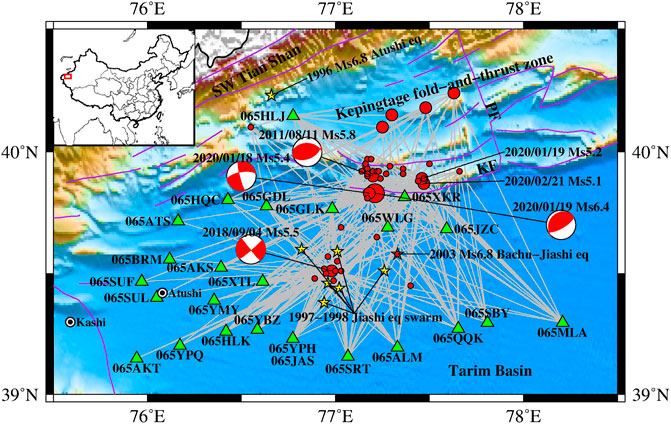
FIGURE 1. Locations of earthquakes (circles) and stations (triangles) considered in the spectral inversion analysis. The stars represent the major historical earthquakes in the proximity of the seismogenic area. The ray paths from the epicenter to the station are depicted by the gray lines. The focal mechanisms were derived from the United States Geology Survey. Purple lines indicate the active faults, and KF and PF represent the Kepingtage thrust fault and the Piqiang fault, respectively. Insert in the top left corner shows the location of the study region (rectangle).
The 2020 Jiashi seismic sequence occurred on the western segment of the frontal Kepingtage thrust fault, which is exposed west of the north-northwest to south-southeast trending Piqiang fault (Figure 1). The Kepingtage thrust fault is the southernmost margin of the Kepingtage fold-and-thrust zone, Cenozoic compressive structures neoformed above a Paleozoic basal decollement level at a depth of 4–6 km, predominantly thrusting toward the interior of the northwest Tarim Basin to the south (Allen and Vincent, 1999; Turner et al., 2010; Yang et al., 2018; Laborde et al., 2019). Much deeper focal depths implied that this sequence was more likely to occur in the basement structures below the decollement level, rather than the thrust sheets that grew above the decollement level (Gao et al., 2013; Laborde et al., 2019).
The high seismic activity in the junction of the northwest Tarim Basin and Kepingtage fold-and-thrust zone was majorly driven by the compressive stresses transmitted by the undeformed rigid Tarim block far to the north from the continental collision of the Indian and Eurasian plates (Buslov et al., 2007; Laborde et al., 2019). Consequently, this region has suffered frequently from moderate-to-large earthquakes, e.g., the 1996 Ms 6.9 Atushi earthquake, the 1997–1998 Jiashi earthquake swarm, the 2003 Ms 6.8 Bachu-Jiashi earthquake, the 2011 Ms 5.8 Atushi earthquake, and the 2018 Ms 5.5 Jiashi earthquake (highlighted by stars in Figure 1). This region is thus persistently exposed to a relatively high seismic hazard. The seismic accelerations reached up to 0.20 and 0.30 g (g, gravitational acceleration) in this region according to the latest generation of seismic ground motion parameter zonation maps of China (GB 18306, 2015).
Studies associated with the earthquake source were of decisive importance for a deep understanding of the seismic source physics and reliable prediction of future ground motions and seismic hazards. The observed ground motion recordings have been commonly utilized in a number of established methods (e.g., empirical Green’s function-based method and large-scale stacking and generalized inversion techniques) aimed at revealing the earthquake source characteristics, e.g., the earthquake source scaling (Allmann and Shearer, 2009; Viegas et al., 2010; Baruah et al., 2016; Trugmann and Shearer, 2017; Baltay et al., 2019) and the source rupture directivity (Abercrombie et al., 2017; Calderoni et al., 2017; Wang et al., 2018). The source characteristics have important implications for explaining the earthquake nucleation and growth (e.g., Moyer et al., 2018).
A dense strong ground motion observation network composed of 48 stations has been constructed and continuously operated since 2007 to monitor the seismic activity in the junction of the southwest Tian Shan and the northwest Tarim Basin. During the 2020 Jiashi seismic sequence, the strong ground motion observation network was progressively triggered by 24 earthquakes and collected a total of over 200 three-component (i.e., east-west, north-south, and up-down) ground motion acceleration recordings. Before this sequence, the observation network had accumulated ∼300 recordings from ∼40 earthquakes, including the 2018 Jiashi seismic sequence, which mainly occurred on the buried faults in the northwest Tarim Basin (Song et al., 2019) and the Kepingtage thrust fault. The buried faults have been verified to be the seismogenic structures of the 1997–1998 Jiashi earthquake swarm (Liu et al., 2000; Li et al., 2002). The Jiashi seismic sequences in both 2020 and 2018 were characterized by the foreshock-mainshock behavior.
In this study, the nonparametric spectral inversion analysis of the S-wave Fourier amplitude spectra of the observed ground motions was performed to isolate the path attenuation and the source spectra for 46 earthquakes considered in this region, including 20 events from the 2020 Jiashi seismic sequence. The source parameters were derived from the inverted source spectra according to the grid-searching method. The resultant stress drop estimates provided the crucial evidence for the source scaling, and the temporal variation in stress drop was further analyzed and used to explain the occurrence of multiple moderate events in the Jiashi seismic sequence.
Dataset
For the spectral inversion analysis, we first collected a total of 502 three-component acceleration waveforms well recorded at 48 strong-motion observation stations from 59 M 2.8 to 6.4 earthquakes occurring in proximity to the seismogenic area of the 2020 Jiashi seismic sequence since 2007. As shown in Figure 2, the hypocentral distances (R) of recordings were mainly in the range of 20–200 km, and the horizontal peak ground accelerations (PGAs) were not greater than 50 cm/s2 for most recordings. These recordings were uniformly processed by the baseline correction, appending zero pads to the beginning and end, and a Butterworth bandpass filter. The high-cut corner frequency was uniformly set to 30 Hz, while the low-cut corner frequency (flc) was preliminarily estimated by two empirical relations and further adjusted and determined after manual inspection. Both empirical relations include the lower boundary (flb) for the usable frequency band associated with the moment magnitude (Mw) imposed by Yenier and Atkinson (2015) based on the minimum usable frequencies reported in the Next Generation Attenuation-West2 (NGA-West2) database and flc associated with flb, i.e., flb = 1.25flc (Abrahamson and Silva, 1997). Here, the magnitudes (surface magnitude Ms or local magnitude ML) released by CENC were approximately regarded as Mw for the preliminary estimate of flc. The determined flc values were in the range of 0.10–0.95 Hz. In order to avoid the nonlinear soil behavior potentially occurring under strong ground shaking (Beresnev and Wen, 1996; Wu et al., 2010) and reduce the contamination of the surface wave and/or Lg wave to the applied S-wave as much as possible (McNamara et al., 2012; Sedaghati et al., 2019), recordings with R > 120 km or PGA > 100 cm/s2 were first eliminated. Moreover, to ensure data redundancy, we adopted a minimum three-recording criterion requiring each selected earthquake to be recorded by at least three selected stations, each of which recorded at least three selected earthquakes. Following these parameters, 116 recordings were eliminated, and we retained 386 ones recorded at 25 stations in 52 M 2.8–6.4 earthquakes.
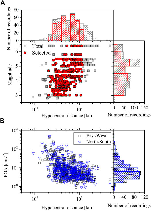
FIGURE 2. (A) Hypocentral distance vs. magnitude for the total recordings collected in this region (squares) and the recordings selected for the spectral inversion analysis (circles). The histograms of the hypocentral distance and the magnitude of the total recordings and selected recordings are also plotted. (B) Peak ground accelerations (PGAs) of both horizontal components (east-west and north-south) for total recordings and the histograms of the horizontal PGAs.
We manually picked the P- and S-wave onsets and identified the S-wave end time according to the distance-dependent percentage of the seismic wave energy, i.e., 90% for R < 25 km, 80% for R = 25–50 km, and 70% for R > 50 km (Pacor et al., 2016). In order to guarantee an acceptable spectral resolution, the minimum length of the S-wave window was imposed as 1.0/(1.25 flc). The cosine tapers at the beginning and end of the extracted S-wave were applied to avoid truncation effects, and the length of each taper was 10% of the length of the S-wave window. The Fourier amplitude spectra of the cosine-tapered and zero-padded S-waves were calculated and smoothed using the window function of Konno and Ohmachi (1998) with smoothing parameter b equal to 20. The spectral amplitudes at 300 frequencies uniformly spaced on the logarithmic scale from 0.25 to 30 Hz were obtained by linear interpolation in log-log space. The root square average of the spectral amplitude at both horizontal components was regarded as the horizontal ground motion in the frequency domain.
The pre-P-wave noise window, sharing the same length of the S-wave window, was extracted and processed, and its Fourier amplitude spectrum was calculated and smoothed for the following calculation of the signal-to-noise ratio (SNR). An SNR threshold of five and flc were simultaneously considered to distinguish the usable frequency band of the S-wave spectra. Figure 3A plots the number of usable spectra and the minimum hypocentral distance (R0) of the usable spectra against frequency. It was clearly observed that the number of usable spectra increases gradually at frequencies of 0.25–1.0 Hz and then approximately keeps constant at frequencies of 1.0–20.0 Hz before a decreasing tendency appears with frequencies over 20.0 Hz. The R0 of the usable spectra also varied with the frequency, which showed smaller values at higher frequencies, i.e., 25.75 km at 0.25 Hz, 20.33 km at 0.254–0.373 Hz, 20.01 km at 0.379–0.431 Hz, 15.02 km at 0.434–0.991 Hz, 12.86 km at 1.007–1.056 Hz, and 9.17 km at 1.073–30 Hz. In order to balance R0 and the lowest usable frequency, R0 = 20.33 km was used. and eight recordings with R < R0 were eliminated. The minimum three-recording criterion was then performed for usable spectra at each frequency to reconstruct the spectra used for the following spectral inversion analysis, and the numbers of usable spectra against frequency are shown in Figure 3B. Finally, 366 recordings recorded at 25 stations in 46 M 3.0–6.4 earthquakes were applied for spectral inversion analysis. Earthquakes and stations considered, as well as the ray paths from earthquake to station, are plotted in Figure 1. The magnitude-hypocentral distance distribution for recordings under consideration is plotted in Figure 2A.
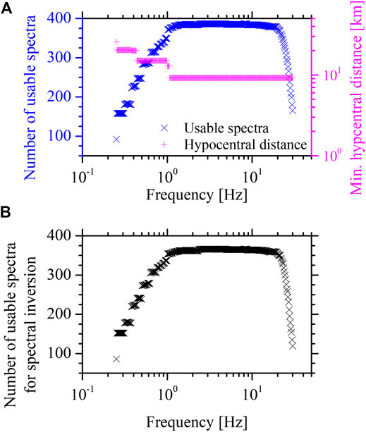
FIGURE 3. (A) The number of usable spectra and minimum hypocentral distance of usable spectra varied with the frequency. (B) The number of usable spectra at each frequency for the recordings selected for the spectral inversion analysis.
Methodology
The two-step nonparametric spectral inversion method (Castro et al., 1990; Oth et al., 2008; Oth et al., 2009) was applied to isolate the Fourier amplitude spectra of the S-waves into the source spectra, site response functions, and propagation path attenuation term.
In the first step, the dependence of the spectral amplitudes at frequency fm on the hypocentral distance is modeled by
where Oij (fm, Rij) is the spectral amplitude observed at the jth station resulting from the ith earthquake, Rij is the hypocentral distance between the jth station and the ith earthquake, Mi (fm) is a scalar dependent on the size of the ith earthquake, and Aij (fm, Rij) accounts for seismic wave attenuation (geometrical spreading, anelastic attenuation and scattering attenuation, refracted arrivals, etc.) along the travel path from the ith earthquake to the jth station. The path attenuation term is not supposed to have any predefined parametric functional form and is constrained to be a smooth distance function with a value of one at the reference distance R0 = 20.33 km, which is the smallest hypocentral distance for recordings considered in our study. In practice, the hypocentral distance of the usable spectra at frequency fm was divided into ND,m bins with 5 km width, and Ak (fm, Rk,m) instead of Aij (fm, Rij) was computed, where Rk,m represents the average hypocentral distance of the usable spectra at frequency fm lying within the kth distance bin. After taking the logarithm for linearization and adding constraints for path attenuation term, Eq. 1 can be solved for each frequency separately using the singular value decomposition (SVD) method.
In the second step, the spectral amplitudes corrected for propagation path attenuation are divided into source spectra and site response:
where Gj (fm) is the site response function at the jth station and Si (fm) is the source spectrum of the ith earthquake.
In order to resolve a remaining degree of freedom coming from the trade-offs between source and site terms, the constraining condition for either the source or the site should be fixed beforehand. The most commonly used method was to set the site response of an ideal outcrop bedrock site to be equal to unity irrespective of frequency (Wang et al., 2018), or to set the average site response of a set of rock sites to be equal to unity (Oth et al., 2009; Oth and Kaiser, 2014; Pacor et al., 2016) or the horizontal-to-vertical (H/V) spectral ratio of body waves (Bindi et al., 2004; Wang et al., 2018). The site conditions for the 25 strong-motion stations considered in this study were classified into three classes defined in the Code for Seismic Design of Buildings in China (GB 50011, 2010) according to the terrain-based metrics (Shi, 2009), 16 for class II (medium-stiff soil), eight for class III (medium soft soil), and one for class IV (soft soil); thus, no one can be approximately regarded as a rock site.
As reported by Lermo and Chavez-Garcia (1993), the H/V spectral ratio of the body waves was largely controlled by the site response. Further studies from Atkinson and Cassidy (2000) and Atkinson (2004) found that the amount of amplification observed or calculated from the shear-wave velocity gradient approximately matches the H/V spectral ratio for both the rock and the soil sites. Kanbur et al. (2020) evaluated the local site effects according to the H/V spectral ratios. Bindi et al. (2004) defined the site response for station ASSI to be the H/V spectral ratio for the spectral inversion. In this study, the H/V spectral ratio was also treated as the site response. The S-wave H/V spectral ratio for each class II site was computed based on the ground motion recordings with PGA ≤ 100 cm/s2, and the average over at least five H/V spectral ratios was approximately regarded as the site response. Finally, the site responses for 10 out of 16 stations were retrieved and plotted in Figure 4A. The site response of the class II site was simply depicted by a range of the average plus and minus 0.25 SD over the 10 stations, shown with the shaded area in Figure 4A. At each frequency, stations with site responses falling into the range of the site response of the class II site were selected as shown in Figure 4B, and the average site response over the selected stations was used as the constraining condition.
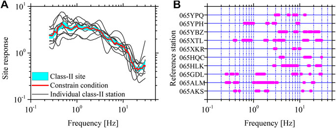
FIGURE 4. (A) The site responses for 10 class II stations (thin gray lines) were represented by the average of the S-wave horizontal-to-vertical spectral ratios of ground motion recordings with peak ground acceleration not greater than 100 cm/s2. A range of the average plus and minus 0.25 SD on the base-10 logarithmic scale over the 10 stations (shaded area) represents the site response of the class II site. At each frequency, stations with site responses falling into the range of the site response of the class II site were selected, and their average site response was used as the constraining condition (thick red line). (B) The selected stations for the constraining condition varied with frequency.
Results and Discussion
Propagation Path Attenuation
Path attenuation curves for frequencies ranging from 0.254 to 30 Hz were obtained from the solutions of Eq. 1 and plotted in Figure 5A. They continuously decrease with increasing distance up to 120 km for all frequencies considered. The slow decay is obviously expressed by the inverted path attenuation, which is generally between (R0/R)0.5 and (R0/R)1.0. For simplicity, the frequency-independent geometrical spreading as a function of distance and the anelastic attenuation as a function of frequency-dependent quality factor (Q) were commonly adopted as substitutes for the complex path attenuation in practice, e.g., the ground motion prediction (e.g., Boore, 2003; Bora et al., 2015) and regional attenuation investigation (e.g., Pavel and Vacareanu, 2018). In addition to the linear function of R, the more complicated geometrical spreading functional forms were widely proposed to represent the particular geologic and tectonic setting, e.g., the hinged bilinear and trilinear models (Atkinson and Boore, 1995; Atkinson, 2004). Studies, e.g., Mahani and Atkinson (2012), verified that various geometrical spreading models have similar effects on fitting the data. Atkinson and Mereu (1992) proposed the typical hinged trilinear model. In this model, the transition distances were related to the crustal thickness. Considering a crustal thickness of ∼50 km (Gao et al., 2013), the second transition distance was about 125 km, greater than the maximum hypocentral distance (i.e., 120 km). In this study, the hinged bilinear geometrical spreading model was used, and the inverted path attenuation curve was modeled by
where β is the shear-wave velocity set to 3.60 km/s at depths of 15–20 km near the source (Zhao et al., 2008), R1 is the transition distance, and n1 and n2 represent the decay rates at the first and second segmentation, respectively. The SVD method was applied to solve Eq. 3 for optimum n1, n2, and Q values by taking different values of transition distance R1 = 50, 55, 60, and 65 km, respectively. Note that the strong trade-off between the geometrical spreading and anelastic attenuation was not constrained before the solution. Therefore, the specified combination of geometrical spreading and anelastic attenuation obtained in this study should be used simultaneously.
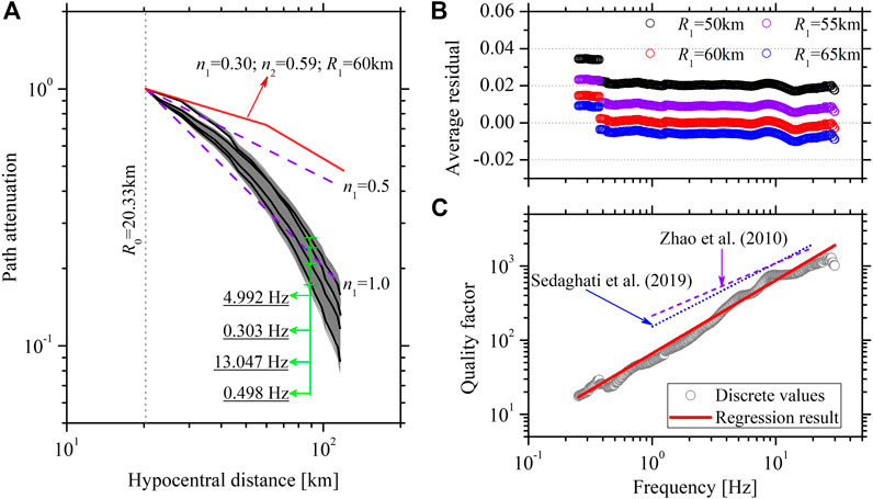
FIGURE 5. (A) The path attenuation curves derived for frequencies at 0.254–30 Hz. The hinged bilinear geometrical spreading model with the transition distance R1 = 60 km provided in this study is plotted and compared with the geometrical spreading models expressed as (R0/R)0.5 and (R0/R)1.0. (B) The average residual between the inverted and the modeled path attenuations over all distances for each frequency with transition distances of R1 = 50, 55, 60, and 65 km, respectively. (C) Calculated Q values (circles) and the regressed Q model (solid line) in our study. The Q models for the northwest Tarim Basin proposed by Zhao et al. (2011) and the Tajikistan-Kyrgyzstan region west and northwest of our study region proposed by Sedaghati et al. (2019) are also plotted.
The residuals between the inverted and modeled path attenuations, i.e., log10 (Ainverted/Amodeled), were calculated to explain whether the inverted path attenuation was well fitted with respect to the parametric functions. The average residual over all distances was obtained for each frequency, as shown in Figure 5B. The minimum average residual, fluctuating around zero, occurs at frequencies over ∼0.3 Hz for the case of R1 = 60 km. The parametric functions for R1 = 50 and 55 km generally provide a faster decay than the inverted path attenuations at frequencies over ∼0.3 Hz, as indicated by the positive average residuals, while slower decay was provided by the parametric functions for R1 = 65 km. Allowing for the good representation of the inverted attenuation curve, R1 = 60 km was recommended in this study. Correspondingly, n1 and n2 are, respectively, equal to 0.30 and 0.59. The derived hinged bilinear geometrical model was slightly larger than the linear geometrical spreading expressed by (R0/R)0.5 (Figure 5A). The frequency-dependent Q model, following a power-law equation expressed as Q0fη, was used to fit the derived Q values at frequencies of 0.254–30 Hz, and the Q model was regressed as 60.066 f0.988, as shown in Figure 5C. The low Q0 and high-frequency-dependent power η can be explained by the seismically active region considered in this study (Xu et al., 2010; Singh et al., 2019). Our results are slightly lower than the S-wave quality factor Q = 212.6 f0.71 at frequencies of 1–20 Hz obtained by Zhao et al. (2011) for the northwest Tarim Basin using the hinged trilinear geometrical spreading model proposed by Atkinson and Mereu (1992). After defining a geometrical spreading function as R−1, Sedaghati et al. (2019) also demonstrated strong anelastic attenuation for the Tajikistan-Kyrgyzstan region in Central Asia, west and northwest of our study region, according to the S-wave quality factor Q = 152 f0.856 at frequencies of 1–20 Hz determined by the multiple-station coda normalization method. The much stronger anelastic attenuation (low Q) verified in our study may be majorly attributed to the enormous scattering from the prominent interaction of seismic wave propagation with the highly inhomogeneous crust. The high heterogeneity in the crust beneath the junction of the southwest Tian Shan and the Tarim Basin has been globally recognized, e.g., the well-developed imbricate structures and complex tectonic activity (Allen and Vincent, 1999; Gao et al., 2013; Laborde et al., 2019).
Source Characteristics
The acceleration source spectra for the 46 earthquakes derived from the second-step inversion were plotted in log-log space in Figure 6A. The bootstrap analysis was first adopted to evaluate the stability of the inverted source spectra (Oth et al., 2009; Wang et al., 2018). At each frequency, we performed 100 bootstrap inversions and calculated the inverted source spectra, as shown in Figure 6B for five typical events. The small deviations to the source spectra obtained using the whole dataset indicated the inverted source spectra are stable and well constrained. We generally observed that the source spectra approximately increase proportional to the square of frequency at low frequencies and then display a plateau at moderate frequencies generally less than ∼10 Hz. However, the rapid decay with increasing frequency occurs at high frequencies generally over ∼10 Hz, as has also been observed in other studies, e.g., Oth et al. (2011), Oth and Kaiser (2014), and Nakano et al. (2015). The well-known ω-square source model proposed by Brune (1970) matches well with the spectral shape below the high-end cutoff frequency (fmax). The high-frequency spectral decay observed above fmax is universally considered to be path- and site-dependent at present (Campbell, 2009; Ktenidou et al., 2013; Lai et al., 2016) and modeled by exp (−πfκ) where κ indicates the high-frequency decay parameter. A hinged model, single ω-square source model below fmax, and combining model of the ω-square source model below fmax and the high-frequency decay model above fmax can be adopted to describe the inverted source spectra. Our study did not focus on the high-frequency spectral decay beyond the scope of the present work. Following the ω-square source model (Brune, 1970), the inverted source spectra at frequencies below fmax = 10 Hz were expressed theoretically by
where M0 and fc are the seismic moment and corner frequency, respectively. RΘΦ is the average radiation pattern over a suitable range of azimuths and take-off angles [set to 0.55 according to Boore and Boatwright (1984)], V = 1/√2 represents the partitioning of the total S-wave energy into horizontal components, F = 2 accounts for the free surface amplification effect, and ρ is the density in the vicinity of the source (set to 2,600 kg/m3 according to Zhao et al. (2008)).
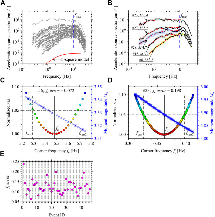
FIGURE 6. (A) Inverted acceleration source spectra for the earthquakes considered; (B) the inverted source spectra from 100 bootstrap inversions (gray, lightblue, and light yellow lines) and the best-fitted theoretical source spectra (red dashed-dotted lines) at frequencies below 10 Hz for five typical events (#10, 20, 27, 40, and 41). The dark lines represent the inverted source spectra using the whole dataset; (C,D) the parabola shapes for the res normalized by the minimum res corresponding to the preferred fc against the possible corner frequencies for #10 and 40 events, respectively. Frequencies at which res exceeds 5% of the minimum res are regarded as fc uncertainty bounds (fcerr1 and fcerr2) to provide fcerror for quantitatively evaluating the parabola shape. The estimated Mw-fc pairs (crosses) for the possible fc are also provided; (E)fcerror values for the considered events. Event ID is listed in Table 1.
The grid-searching method was applied to provide the preferred M0 and fc estimates for individual events that minimize the function
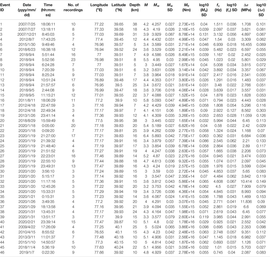
TABLE 1. Basic information for earthquakes under investigation and source parameter estimates.
In order to examine the reliability for estimates by grid searching, we further tested the res against possible fc values for a parabola shape with a clear minimum at the preferred fc. Following Viegas et al. (2010), Abercrombie (2014), and Ruhl et al. (2017), we used frequencies at which the res exceeds 5% of the minimum res as an estimate of the fc uncertainty bounds fcerr1 and fcerr2, and fcerror, defined as the frequency-normalized ratio
Seismic moments for the earthquakes considered range from 1.650 × 10¹⁴ to 7.754 × 10¹⁷ Nm, corresponding to MW = 3.445–5.893. We obtained corner frequencies from 0.362 to 6.940 Hz for these events. Approximately constant earthquake stress drops over a wide range of earthquake sizes and the well-known scaling relation M0 ∝ fc−3 reveal earthquake self-similar scaling, first proposed by Aki (1967). The self-similar scaling has crucial implications for seismic hazard assessment and understanding of the scale dependence of the earthquake rupture process. The self-similarity has been widely reported by many studies (e.g., Allmann and Shearer, 2009; Oth et al., 2010; Oth and Kaiser, 2014; Boyd et al., 2017; Moyer et al., 2018), while other studies have provided evidence for the significant breakdown of self-similarity (e.g., Drouet et al., 2011; Pacor et al., 2016; Baruah et al., 2016; Trugmann and Shearer, 2018). The plots of M0 vs. fc for earthquakes considered in this study intuitively depart from the scaling relation, as shown in Figure 7. Moreover, we applied a so-called parameter ε proposed by Kanamori and Rivera (2004) from the scaling relation M0 ∝ fc−(3+ε) to quantify the deviation from the self-similarity. When ε = 0, it indicates perfect self-similar scaling. We found ε = −0.424 ± 0.122 according to the least-squares regression, which indicates the decrease of stress drop on average with the increasing magnitude size. Similar ε values have also been observed in the 2008 Wenchuan and 2013 Lushan seismic sequences (Wen et al., 2015; Wang et al., 2018), even if the estimated stress drops showed differences (Figure 7).
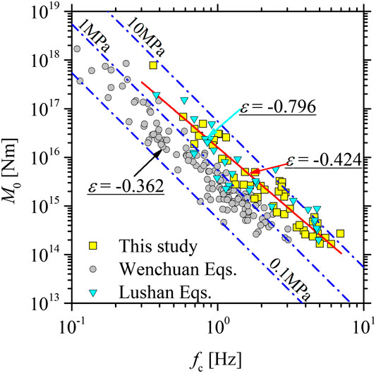
FIGURE 7. Seismic moment (M0) vs. corner frequency (fc). Squares, circles, and triangles represent the earthquakes considered in this study, the 2008 Wenchuan (Wang et al., 2018), and the 2013 Lushan (Wen et al., 2015) seismic sequences, respectively. The M0 ∝ fc−3 scaling relation corresponding to constant stress drops 0.1, 1.0, and 10.0 MPa, respectively, following the theoretical model of Brune (1970), is represented by the dotted-dashed lines.
According to the circular source model (Eshelby, 1957; Brune, 1970), the stress drop Δσ can be obtained from the following formulas:
where r is the fault radius and k is a numerical factor that depends on the specific theoretical model (Brune, 1970; Madariaga, 1976; Kaneko and Shearer, 2014; Kaneko and Shearer, 2015). The selection of the theoretical model predominantly controls the absolute values of Δσ. For example, the two most commonly adopted models proposed by Brune (1970) and by Madariaga (1976) yield a difference for the computed stress drops with a factor of ∼5.5. However, the relative values and the variations in Δσ are not influenced by the model selection. In this study, k = 0.37 was used for S-waves according to the theoretical model of Brune (1970). The combination of M0 and fc yields Δσ values between 1.126 and 16.455 MPa, as shown in Figure 8A. Computed stress drops exhibit large scatter and approximately show a lognormal distribution with an average value of 3.942 MPa and an SD for the stress drop on the base-10 logarithmic scale equal to 0.284. The average stress drop is similar to the global averages for tectonic earthquakes, ∼1–10 MPa (Allmann and Shearer, 2009; Oth et al., 2010; Trugmann and Shearer, 2017; Baltay et al., 2019). Median stress drops show a mild decreasing tendency as a function of moment magnitude over a range Mw = 3.445–5.189, which indicates that self-similar scaling breaks for these earthquakes under investigation. However, there is no dependence of stress drop on the hypocentral depth (Figure 8B). As shown in Figure 8A, except for some events in the 2020 sequence with relatively higher stress drops, earthquakes with similar moment magnitudes from the Jiashi seismic sequences in both 2020 and 2018 generally share a similar level of stress drop (∼1–6 MPa), and stress drops first decrease and then increase with the increasing moment magnitude.
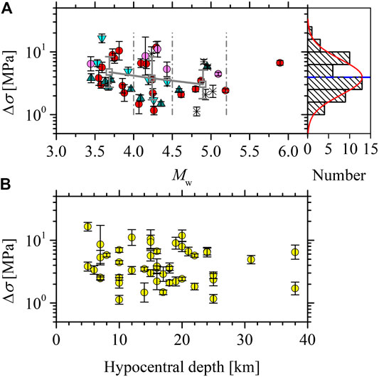
FIGURE 8. Stress drop (Δσ) as a function of moment magnitude (Mw) (A) and hypocentral depth (B). Red circles and dark cyan triangles represent earthquakes in the 2020 and 2018 Jiashi seismic sequences, respectively. Light magenta circles and light cyan triangles represent earthquakes that formerly occurred in proximity to the seismogenic regions of the 2020 and 2018 sequences, respectively. Other earthquakes considered are marked by crosses. The lognormally distributed Δσ values are found from the histogram.
Earthquakes considered in this study mainly consist of the 2020 Jiashi seismic sequence (#21–#40) on the Kepingtage thrust fault and the 2018 Jiashi seismic sequence (#7–#15) on the buried fault in the northwest Tarim Basin. Similar to the 2020 sequence, an Ms 4.9 foreshock immediately followed by the Ms 5.5 mainshock aroused the 2018 sequence. Figure 9 provides the temporal variation of stress drop estimates for both sequences. In or close to the seismogenic regions of both sequences, some sporadic small earthquakes occurred months to years before the sequence with relatively higher stress drops compared with aftershocks with a similar moment magnitude (Figures 8A, 9), while the foreshocks minutes to days before the mainshock released much lower stress, consistent with the observations from other earthquake sequences (e.g., Moyer et al., 2018). After the stress drop returned to the higher level during the adjoining mainshock, aftershocks immediately following in close proximity to the mainshock showed depressing stress drops in both sequences, which furnishes a potential clue of the continuous rerupture of the already fractured and not fully healed portion by the mainshock (Shaw et al., 2015). Aftershocks with stress drops much smaller than the mainshock have also been commonly reported for both tectonic and induced seismic sequences (e.g., Boyd et al., 2017; Trugman et al., 2017; Moyer et al., 2018; Trugmann and Shearer, 2018; Baltay et al., 2019) and used to account for the reduced ground motion of aftershocks (Abrahamson et al., 2014). The stress drops of the aftershocks appeared to recover gradually as time increased, which was also observed in the induced seismic sequences (e.g., Trugman et al., 2017; Yenier et al., 2017). Such temporal recovery of the stress drop may be indicative of an increase of fault strength with the increase in healing time. Finally, the released stress was elevated to a rather high level, even over 10 MPa for partial aftershocks, which subsequently occurred 10 h to days later in the 2020 sequence, which hints to potential ruptures for the isolated, small-scale patches with high strength concentrating substantial stress levels in the damaged fault zone (Dreger et al., 2007; Oth and Kaiser, 2014). The changes of the fault strength across the seismogenic fault caused by the mainshock play short-term roles on sources of the surrounding earthquakes.
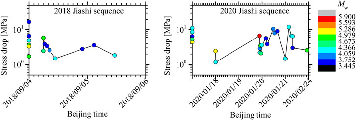
FIGURE 9. Temporal variation of stress drops for the 2018 and 2020 Jiashi seismic sequences. Earthquakes previously occurring close to the seismogenic region are plotted in the vertical axis; #1–#6 and #16–#20 represent the 2018 and 2020 sequences, respectively.
In both sequences, the strong foreshock did not ultimately expand to be the largest mainshock. In view of the low stress drop of the foreshock and the high stress release in the adjoining mainshock, we presumed that the adjoining high-strength patch eventually ruptured by the mainshock may cease the continuous expansion of the fractured low-strength patch by the foreshock. Moreover, the initiating fracture of the low-strength patch may play an effective role in accelerating the concentration of stress at the edge of the high-strength patch (Oth and Kaiser, 2014), until the high-strength patch broke to account for the mainshock. As concluded by Ben-Zion and Zhu (2002), large earthquakes grow in a relatively homogeneous stress field and average out the remaining short-scale fluctuations over their (large) rupture areas. We thus inferred that the foreshock-mainshock behavior may be likely to occur in the high heterogeneous fault zone.
Conclusion
We performed the nonparametric spectral inversion to isolate the propagation path attenuation and source spectra from the S-wave Fourier amplitude spectra of the observed ground motions from 46 earthquakes in the junction of the northwest Tarim Basin and Kepingtage fold-and-thrust zone, mainly composed of two Jiashi seismic sequences in 2020 and 2018. Nonparametric path attenuation curves indicate slow seismic wave decay with increasing hypocentral distance. The path attenuation was simply modeled by the combination of the hinged bilinear geometrical model and the anelastic attenuation model as a function of the quality factor. The combination derived in this study can be directly used for predicting ground motions in this region. The transition distance R1 = 60 km, n1 = 0.30, and n2 = 0.59 defined the preferred hinged bilinear geometrical model in the study region. The strong anelastic attenuation in the study region, represented by Q = 60.066 f0.988 at frequencies of 0.254–30 Hz, may be ascribed to enormous scattering resulting from the prominent interaction of seismic wave propagating with the high inhomogeneous crust.
The inverted source spectra at frequencies below fmax = ∼10 Hz are found in good agreement with the ω-square model; the source parameters were thus estimated by fitting the inverted spectra with the theoretical ω-square model. The obvious deviation of M0-fc plots to the M0 ∝ fc−3 scaling relation and the dependence of the stress drop on the moment magnitude provide crucial evidence for the breakdown of earthquake self-similar scaling for the events considered in this study. The stress drops for earthquakes from the Jiashi seismic sequences in both 2020 and 2018 appear to first decrease and then increase as the moment magnitude increased. The average stress drop for these earthquakes was 3.942 MPa. The temporal variation of the stress drops indicates the short-term effects of the mainshock on the source characteristics of the adjoining earthquakes before and after the mainshock. After the great stress release during the mainshock, the stress drops fell to a low level for aftershocks immediately following and then gradually recovered in a short time, which reveals the gradual healing of the fractured fault by the mainshock. The much higher stress drops for some aftershocks in the damaged fault zone may also be related to the potential ruptures for small-scale patches with high strength. The foreshock with a low stress release occurring in the high-heterogeneity fault zone may motivate the following occurrence of the largest magnitude mainshock with a high stress release. We inferred that the foreshock-mainshock behavior may be inclined to occur in the inhomogeneous fault zone, e.g., the junction of the northwest Tarim Basin and Kepingtage fold-and-thrust zone.
Data Availablity Statement
Publicly available datasets were analyzed in this study. This data can be found here: Ground motion recordings for this study were provided by China Strong Motion Network Centre at Institute of Engineering Mechanics, China Earthquake Administration, contacting the email Y3NtbmNAaWVtLmFjLmNu for data application (last accessed March 2020). Basin information for earthquakes mentioned in this study was obtained from China Earthquake Network Center at the website of http://news.ceic.ac.cn/ (last accessed March 2020). The focal mechanisms for some earthquakes in this study were derived from the United States Geology Survey at the website of www.usgs.gov/ (last accessed February 2020).
Author Contributions
HW and RW worked together for this manuscript. They jointly collected and processed the strong ground motion recordings for the observed S-wave spectra. HW performed the nonparametric spectral inversion for isolating the propagation path attenuation and the source spectra. HW and RW estimated the source parameters and evaluated their reliability and uncertainty. They analyzed the temporal variation of stress drop and drew some interesting conclusions. They together wrote this article.
Funding
This work was supported by the National Natural Science Foundation of China (nos. 51808514; 51878632) and the Science Foundation of the Institute of Engineering Mechanics, China Earthquake Administration (no. 2018B03).
Conflict of Interest
The authors declare that the research was conducted in the absence of any commercial or financial relationships that could be construed as a potential conflict of interest.
References
Abercrombie, R. E. (2014). Stress drops of repeating earthquakes on the San Andreas fault at Parkfield. Geophys. Res. Lett. 41, 8784–8791. doi:10.1002/2014GL062079
Abercrombie, R. E., Bannister, S., Ristau, J., and Doser, D. (2017). Variability of earthquake stress drop in a subduction setting, the Hikurangi margin, New Zealand. Geophys. J. Int. 208, 306–320. doi:10.1093/gji/ggw393
Abrahamson, N. A., and Silva, W. J. (1997). Empirical response spectral attenuation relations for shallow crustal earthquakes. Seismol Res. Lett. 68 (1), 94–127. doi:10.1785/gssrl.68.1.94
Abrahamson, N. A., Silva, W. J., and Kamai, R. (2014). Summary of the ASK14 ground-motion relation for active crustal regions. Earthquake Spectra 30 (3), 1025–1055. doi:10.1193/070913EQS198M
Aki, K. (1967). Scaling law of seismic spectrum. J. Geophys. Res. 72 (4), 1217–1231. doi:10.1029/JZ072i004p01217
Allen, M. B., and Vincent, S. J. (1999). Late Cenozoic tectonics of the Kepingtage thrust zone: interactions of the Tien Shan and Tarim Basin, northwest China. Tectonics 18 (4), 639–645. doi:10.1029/1999TC900019
Allmann, B. P., and Shearer, P. M. (2009). Global variations of stress drop for moderate to large earthquakes. J. Geophys. Res. 114, B01310. doi:10.1029/2008JB005821
Atkinson, G. M. (2004). Empirical attenuation of ground-motion spectral amplitudes in southeastern Canada and the northeastern United States. Bull. Seismol. Soc. Am. 94 (3), 1079–1095. doi:10.1785/0120040161
Atkinson, G. M., and Boore, D. M. (1995). Ground-motion relation for eastern North America. Bull. Seismol. Soc. Am. 85 (1), 17 –30.
Atkinson, G. M., and Cassidy, J. F. (2000). Integrated use of seismography and strong-motion data to determine soil amplification: response of the Fraser River Delta to the Duvall and Georgia Strait earthquakes. Bull. Seismol. Soc. Am. 90 (4), 1028–1040. doi:10.1785/0119990098
Atkinson, G. M., and Mereu, R. F. (1992). The shape of ground motion attenuation curves in southeastern Canada. Bull. Seismol. Soc. Am. 82 (5), 2014–2031.
Baltay, A. S., Hanks, T. C., and Abrahamson, N. A. (2019). Earthquake stress drop and Arias intensity. J. Geophys. Res. Solid Earth 124, 3838–3852. doi:10.1029/2018JB016753
Baruah, B., Kumar, P., Kumar, M. R., and Ganguli, S. S. (2016). Stress-drop variations and source scaling relations of moderate earthquakes of the Indian tectonic plate. Bull. Seismol. Soc. Am. 106 (6), 2640–2652. doi:10.1785/0120150106
Ben-Zion, Y., and Zhu, L. (2002). Potency–magnitude scaling relations for southern California earthquakes with 1.0 < ML < 7.0. Geophys. J. Int. 148, F1–F5. doi:10.1046/j.1365-246X.2002.01637.x
Beresnev, I. A., and Wen, K.-L. (1996). Nonlinear soil response—a reality. Bull. Seismol. Soc. Am. 86 (6), 1964–1978.
Bindi, D., Castro, R. R., Franceschina, G., Luzi, L., and Pacor, F. (2004). The 1997–1998 Umbria–Marche sequence (Central Italy): source, path, and site effects estimated from strong motion data recorded in the epicentral area. J. Geophys. Res. 109, B04312. doi:10.1029/2003JB002857
Boore, D. M. (2003). Simulation of ground motion using the stochastic method. Pure Appl. Geophys. 163, 635–676.
Boore, D. M., and Boatwright, J. (1984). Average body-wave radiation coefficients. Bull. Seismol. Soc. Am. 74 (5), 1615–1621.
Bora, S. S., Scherbaum, F., Kuehn, N., Stafford, P., and Edwards, B. (2015). Development of a response spectral ground-motion prediction equation (GMPE) for seismic-hazard analysis from empirical Fourier spectra and duration models. Bull. Seismol. Soc. Am. 105 (4), 2192–2218. doi:10.1785/0120140297
Boyd, O. S., McNamara, D. E., Hartzell, S., and Choy, G. (2017). Influence of lithostatic stress on earthquake stress drops in North America. Bull. Seismol. Soc. Am. 107 (2), 856–868. doi:10.1785/0120160219
Brune, J. N. (1970). Tectonic stress and the spectra of seismic shear waves from earthquakes. J. Geophys. Res. 75 (26), 4997–5009. doi:10.1029/JB075i026p04997
Buslov, M. M., Grave, J. D., Bataleva, E. A. V., and Batalev, V. Y. (2007). Cenozoic tectonic and geodynamic evolution of the Kyrgyz Tien Shan Mountains: a review of geological, thermochronological, and geophysical data. J. Asian Earth Sci. 29, 205–214. doi:10.1016/j.jseaes.2006.07.001
Calderoni, G., Rovelli, A., and Giovambattista, R. D. (2017). Rupture directivity of the strongest 2016–2017 central Italy earthquakes. J. Geophys. Res. Solid Earth 122 (11), 9118–9131. doi:10.1002/2017JB014118
Campbell, K. W. (2009). Estimates of shear-wave Q and κ0 for unconsolidated and semiconsolidated sediments in eastern North America. Bull. Seismol. Soc. Am. 99 (4), 2365–2392. doi:10.1785/0120080116
Castro, R. R., Anderson, J. G., and Singh, S. K. (1990). Site response, attenuation and source spectra of S waves along the Guerrero, Mexica, subduction zone. Bull. Seismol. Soc. Am. 80 (6), 1481–1503.
Dreger, D., Nadeau, R. M., and Chung, A. (2007). Repeating earthquakes finite source models: strong asperities revealed on the San Andreas fault. Geophys. Res. Lett. 34, L23302. doi:10.1029/2007gl031353
Drouet, S., Bouin, M.-P., and Cotton, F. (2011). New moment magnitude scale, evidence of stress drop magnitude scaling and stochastic ground motion model for the French West Indies. Geophys. J. Int. 187, 1625–1644. doi:10.1111/j.1365-246X.2011.05219.x
Eshelby, J. D. (1957). The determination of the elastic field of an ellipsoidal inclusion, and related problems. Proc. R. Soc. Lond. 241 (1226), 376–396. doi:10.1098/rspa.1957.0133
Gao, R., Hou, H., Cai, X., Hnapp, J. H., He, R., Liu, J., et al. (2013). Fine crustal structure beneath the junction of the southwest Tian Shan and Tarim Basin, NW China. Lithosphere 5, 382–392. doi:10.1130/L248.1
Hanks, T. C., and Kanamori, H. (1979). A moment magnitude scale. J. Geophys. Res. 84, 2348–2350. doi:10.1029/JB084iB05p02348
Kanamori, H., and Rivera, L. (2004). Static and dynamic scaling relations for earthquakes and their implications for rupture speed and stress drop. Bull. Seismol. Soc. Am. 94 (1), 314–319. doi:10.1785/0120030159
Kanbur, M. Z., Silahtar, A., and Aktan, G. (2020). Local site effects evaluation by surface wave and H/V survey methods in Senirkent (Isparta) region, southwestern Turkey. Earthq. Eng. Eng. Vib. 19, 321–333. doi:10.1007/s11803-020-0564-z
Kaneko, Y., and Shearer, P. M. (2014). Seismic source spectra and estimated stress drop derived from cohesive-zone models of circular subshear rupture. Geophys. J. Int. 197, 1002–1015. doi:10.1093/gji/ggu030
Kaneko, Y., and Shearer, P. M. (2015). Variability of seismic source spectra, estimated stress drop, and radiated energy, derived from cohesive-zone models of symmetrical and asymmetrical circular and elliptical ruptures. J. Geophys. Res. Solid Earth 120, 1053–1079. doi:10.1002/2014JB011642
Konno, K., and Ohmachi, T. (1998). Ground-motion characteristics estimated from ratio between horizontal and vertical components of microtremor. Bull. Seismol. Soc. Am. 88 (1), 228–241.
Ktenidou, O.-J., Gélis, C., and Bonilla, L.-F. (2013). A study on the variability of kappa (κ) in a borehole: implications of the computation process. Bull. Seismol. Soc. Am. 103 (2A), 1048–1068. doi:10.1785/0120120093
Laborde, A., Barrier, L., Simoes, M., Li, H., Coudroy, T., Woerd, J. V. D., et al. (2019). Cenozoic deformation of the Tarim Basin and surrounding ranges (Xinjiang, China): a regional overview. Earth Sci. Rev. 197, 102891. doi:10.1016/j.earscirev.2019.102891
Lai, T.-S., Mittal, H., Chao, W.-A., and Wu, Y.-M. (2016). A study on kappa value in Taiwan using borehole and surface seismic array. Bull. Seismol. Soc. Am. 106 (4), 1509–1517. doi:10.1785/0120160004
Lermo, J., and Chavez-Garcia, F. (1993). Site effect evaluation using spectral ratios with only one station. Bull. Seismol. Soc. Am. 83, 1574–1594.
Li, S., Zhang, X., Mooney, W. D., and Lai, X. (2002). A preliminary study on the structures of Jiashi earthquake region and earthquake generating fault. Chin. J. Geophys. 45 (1), 76–82 [in Chinese, with English summary].
Liu, Q., Chen, J., Li, S., and Guo, B. (2000). Passive seismic experiment in Xinjiang-Jiashi strong earthquake region and discussion on its seismic genesis. Chin. J. Geophys. 43 (3), 356–365 [in Chinese, with English summary]. doi:10.1002/cjg2.48
Madariaga, R. (1976). Dynamics of an expanding circular fault. Bull. Seismol. Soc. Am. 66 (3), 639–666.
Mahani, A. B., and Atkinson, G. M. (2012). Evaluation of functional forms for the attenuation of small-to-moderate earthquake response spectral amplitudes in North America. Bull. Seismol. Soc. Am. 102 (6), 2714–2726. doi:10.1785/0120120050
McNamara, D., Meremonte, M., Maharrey, J. Z., Mildore, S.-L., Altidore, J. R., Anglade, D., et al. (2012). Freqeuncy-dependent seismic attenuation within the Hispaniola Island region of the Caribbean sea. Bull. Seismol. Soc. Am. 102 (2), 773–782. doi:10.1785/0120110137
Moyer, P. A., Boettcher, M. S., McGuire, J. J., and Collins, J. A. (2018). Spatial and temporal variations in earthquake stress drop on Gofar transform fault, east Pacific Rise: implications for fault strength. J. Geophys. Res. Solid Earth 123, 7722–7740. doi:10.1029/2018jb015942
Nakano, K., Matsushima, S., and Kawase, H. (2015). Statistical properties of stromg ground motions from the generalized spectral inversion of data observed by K-NET, KiK-net and the JMA Shindokei Network in Japan. Bull. Seismol. Soc. Am. 105 (5), 2662–2680. doi:10.1785/0120140349
Oth, A., Bindi, D., Parolai, S., and Giacomo, D. D. (2011). Spectral analysis of K-NET and KiK-net data in Japan, Part II: on attenuation characteristics, source spectra, and site response of borehole and surface stations. Bull. Seismol. Soc. Am. 102 (2), 667–687. doi:10.1785/0120100135
Oth, A., Bindi, D., Parolao, S., and Giacomo, D. D. (2010). Earthquake scaling characteristics and the scale-(in)dependence of seismic energy-to-moment ratio: insights from KiK-net data in Japan. Geophys. Res. Lett. 37 (19), 470–479. doi:10.1029/2010GL044572
Oth, A., Bindi, D., Parolai, S., and Wenzel, F. (2008). S-wave attenuation characteristics beneath the Vrancea region in Romania: new insights from the inversion of ground-motion spectra. Bull. Seismol. Soc. Am. 98 (5), 2482–2497. doi:10.1785/0120080106
Oth, A., and Kaiser, A. E. (2014). Stress release and source scaling of the 2010–2011 Canterbury, New Zealand earthquake sequence from spectral inversion of ground motion data. Pure Appl. Geophys. 171, 2767–2782. doi:10.1007/s00024-013-0751-1
Oth, A., Parolai, S., Bindi, D., and Wenzel, F. (2009). Source spectra and site response from S waves of intermediate-depth Vrancea, Romania, earthquakes. Bull. Seismol. Soc. Am. 99 (1), 235–254. doi:10.1785/0120080059
Pacor, F., Spallarossa, D., Oth, A., Luzi, L., Puglia, R., Cantore, L., et al. (2016). Spectral models for ground motion prediction in the L’Aquila region (central Italy): evidence for stress-drop dependence on magnitude and depth. Geophys. J. Int. 204, 697–718. doi:10.1093/gji/ggv448
Pavel, F., and Vacareanu, R. (2018). Investigation on regional attenuation of Vrancea (Romania) intermediate-depth earthquakes. Earthq. Eng. Eng. Vib. 17, 501–509. doi:10.1007/s11803-018-0458-5
Ruhl, C. J., Abercrombie, R. E., and Smith, K. D. (2017). Spatiotemporal variation of stress drop during the 2008 Mogul, Nevada earthquake swarm. J. Geophys. Res. Solid Earth 122 (1), 8163–8180. doi:10.1002/2017JB014601
Sedaghati, F., Nazemi, N., Pezeshk, S., Ansari, A., Daneshvaran, S., and Zare, M. (2019). Investigation of coda and body wave attenuation functions in Central Asia. J. Seismol., 23, 1047–1070. doi:10.1007/s10950-019-09854-x
Shaw, B. E., Richards-Dinger, K., and Dieterich, J. H. (2015). Deterministic model of earthquake clustering shows reduced stress drops for nearby aftershocks. Geophys. Res. Lett. 42, 9231–9238. doi:10.1002/2015GL066082
Shi, D. (2009). Study on new methods of site classification based on GIS. Master’s thesis. Harbin (China): China Earthquake Administration.
Singh, C., Biswas, R., Jaiswal, N., and Kumar, M. R. (2019). Spatial variations of coda wave attenuation in Andaman-Nicobar subduction zone. Geophys. J. Int. 217 (3), 1515–1523. doi:10.1093/gji/ggz098
Song, C., Gao, R., Liu, J., Liu, P., Guo, Y., and Wen, S. (2019). Discussion on earthquake sequence and seismogenic structure for the Jiashi Ms5.5 earthquake on September 4, 2018, Xinjiang. Earthq. Res. China 35 (2), 256–268 [in Chinese, with English summary].
Trugmann, D. T., and Shearer, P. M. (2017). Application of an improved spectral decomposition method to examine earthquake source scaling in southern California. J. Geophys. Res. Solid Earth 122 (4), 2890–2910. doi:10.1002/2017JB013971
Trugmann, D. T., and Shearer, P. M. (2018). Strong correlation between stress drop and peak ground acceleration for M 1-4 earthquakes in the San Francisco Bay area. Bull. Seismol. Soc. Am. 108 (2), 929–945. doi:10.1785/0120170245
Trugman, D. T., Dougherty, S. L., Cochran, E. S., and Shearer, P. M. (2017). Source spectral properties of small-to-moderate earthquakes in southern Kansas. J. Geophys. Res. Solid Earth 122 (10), 8021–8034. doi:10.1002/2017JB014649
Turner, S. A., Cosgrove, J. W., and Liu, J. G. (2010). Controls on lateral structural variability along the Keping Shan Thrust belt, SW Tien Shan Foreland, China. Geol. Soc. Spec. Publ. 348, 71–85. doi:10.1144/SP348.5
Viegas, G., Abercrombie, R. E., and Kim, W.-Y. (2010). The 2002 M5 Au Sable Forks, NY, earthquake sequence: source scaling relationships and energy budget. J. Geophys. Res. Solid Earth 115, B07310. doi:10.1029/2009JB006799
Wang, H., Ren, Y., and Wen, R. (2018). Source parameters, path attenuation and site effects from strong-motion recordings of the Wenchuan aftershocks (2008–2013) using a non-parametric generalized inversion technique. Geophys. J. Int. 212, 872–890. doi:10.1093/gji/ggx447
Wen, R., Wang, H., and Ren, Y. (2015). Estimation of source parameters and quality factor based on the generalized inversion method in Lushan earthquake. J. Harbin Inst. Technol. 47 (4), 58–63. doi:10.11918/j.issn.0367-6234.2015.04.010
Wu, C., Peng, Z., and Ben-Zion, Y. (2010). Refined thresholds for non-linear ground motion and temporal changes of site response associated with medium-size earthquakes. Geophys. J. Int. 182, 1567–1576. doi:10.1111/j.1365-246X.2010.04704.x
Xu, Y., Herrmann, R. B., Wang, C.-Y., and Cai, S. (2010). Preliminary high-frequency ground-motion scaling in Yunnan and southern Sichuan, China. Bull. Seismol. Soc. Am. 100 (5B), 2508–2517. doi:10.1785/0120090196
Yang, Y., Yao, W. Q., Yan, J. J., Guo, Y., and Xie, D. Q. (2018). Mesozoic and Cenzoic structural deformation in the NW Tarim Basin, China: a case study of the Piqiang-Selibuya fault. Int. Geol. Rev. 60 (7), 929–943. doi:10.1080/00206814.2017.1360803
Yenier, E., and Atkinson, G. M. (2015). An equivalent point-source model for stochastic simulation of earthquake ground motions in California. Bull. Seismol. Soc. Am. 105 (3), 1435–1455. doi:10.1785/0120140254
Yenier, E., Atkinson, G. M., and Sumy, D. F. (2017). Ground motions for induced earthquakes in Oklahoma. Bull. Seismol. Soc. Am. 107 (1). doi:10.1785/0120160114
Zhao, C., Chen, Z., Hua, W., Wang, Q., Li, Z., and Zheng, S. (2011). Study on source parameters of small to moderate earthquakes in the main seismic active regions, China mainland. Chin. J. Geophys. 54 (6), 1478–1489. doi:10.3969/j.issn.0001-5733.2011.06.007
Keywords: seismic ground motion, spectral inversion, propagation path attenuation, source spectra, stress drop
Citation: Wang H and Wen R (2020) Earthquake Source Characteristics and S-Wave Propagation Attenuation in the Junction of the Northwest Tarim Basin and Kepingtage Fold-and-Thrust Zone. Front. Earth Sci. 8:567939. doi: 10.3389/feart.2020.567939
Received: 31 May 2020; Accepted: 22 October 2020;
Published: 22 December 2020.
Edited by:
Pier Paolo Bruno, University of Naples Federico II, ItalyReviewed by:
Shuang Li, Harbin Institute of Technology, ChinaR. B. S. Yadav, Kurukshetra University, India
Copyright © 2020 Wang and Wen. This is an open-access article distributed under the terms of the Creative Commons Attribution License (CC BY). The use, distribution or reproduction in other forums is permitted, provided the original author(s) and the copyright owner(s) are credited and that the original publication in this journal is cited, in accordance with accepted academic practice. No use, distribution or reproduction is permitted which does not comply with these terms.
*Correspondence: Ruizhi Wen, cnVpemhpQGllbS5hYy5jbg==