 Tobias Stål
 Anya M. Reading
 Jacqueline A. Halpin
 Steven J. Phipps
 Joanne M. Whittaker
- 1School of Natural Sciences (Earth Sciences/Physics), University of Tasmania, Hobart, TAS, Australia
- 2Institute for Marine and Antarctic Studies, University of Tasmania, Hobart, TAS, Australia
Interdisciplinary research concerning solid Earth–cryosphere interaction and feedbacks requires a working model of the Antarctic crust and upper mantle. Active areas of interest include the effect of the heterogeneous Earth structure on glacial isostatic adjustment, the distribution of geothermal heat, and the history of erosion and deposition. In response to this research need, we construct an adaptable and updatable 3D grid model in a software framework to contain and process solid Earth data. The computational framework, based on an open source software package agrid, allows different data sources to be combined and jointly analyzed. The grid model is populated with crustal properties from geological observations and geochronology results, where such data exist, and published segmentation from geophysical data in the interior where direct observations are absent. The grid also contains 3D geophysical data such as wave speed and derived temperature from seismic tomographic models, and 2D datasets such as gravity anomalies, surface elevation, subglacial temperature, and ice sheet boundaries. We demonstrate the usage of the framework by computing new estimates of subglacial steady-state heat flow in a continental scale model for east Antarctica and a regional scale model for the Wilkes Basin in Victoria Land. We hope that the 3D model and framework will be used widely across the solid Earth and cryosphere research communities.
1. Introduction
Past, present, and future changes in the mass of the Antarctic ice sheets have a direct impact on global sea level (e.g., King et al., 2012; Shepherd et al., 2012; Golledge et al., 2015; Ritz et al., 2015; DeConto and Pollard, 2016; Golledge et al., 2019). During the 21st century and beyond, the projected rise in sea level in response to anthropogenic climate change is expected to have enormous social and economic consequences (e.g., Kulp and Strauss, 2019; Oppenheimer et al., 2019). Constraining the likely response of ice sheets to global climate change is therefore a high priority. The mechanisms controlling the extent and thickness of the cryosphere involve interaction with the atmosphere (e.g., Frieler et al., 2015; DeConto and Pollard, 2016; Lenaerts et al., 2016), the ocean (e.g., DeConto and Pollard, 2016; Dinniman et al., 2016; Rintoul et al., 2016), and the crust and mantle beneath, which is the focus of this contribution. Examples of solid Earth–cryosphere interaction include the impact of the heterogeneous Earth structure on glacial isostatic adjustment (e.g., Whitehouse, 2018), the amount and distribution of geothermal heat (e.g., Pattyn, 2010), and the history of erosion and deposition over geological time (e.g., Paxman et al., 2018). The continental crust is a highly heterogeneous layer usually characterized by a combination of geological observations, geochronological results, tectonic plate reconstructions, and geophysical surveys to obtain an overall picture of the composition, age, evolution, and 3D architecture of its constituent units. A sharp change in seismic wave speed, the Mohorovičić discontinuity (Moho), defines the boundary between the crust and the mantle beneath (Christensen, 1988; An et al., 2015a). The upper mantle provides a rigid and tectonically mobile component, which together with the crust forms the continental lithosphere. A deeper seismic discontinuity, the lithosphere–asthenosphere boundary (LAB), indicates the transition to a ductile mantle as a result of increasing temperature and pressure with depth (Artemieva, 2011). Many aspects of the Earth’s crust and mantle have significant spatial variability that impacts overlying ice sheets; hence, access to solid Earth research results has gained importance to the interdisciplinary research community (Whitehouse et al., 2019).
1.1. Geology, Geochronology, and Geochemistry
Our understanding of the Antarctic crust is restricted by the ice cover that leaves only 0.18% of the rocks exposed (Burton-Johnson et al., 2016), with access further limited by logistical difficulties. Early field campaigns enabled geological investigations to map out crustal domains along the Antarctic coast and Transantarctic Mountains (Ravich et al., 1965; Craddock, 1970; Adie and Adie, 1977; Tingey et al., 1991). Those interpretations are, to a large extent, still valid, although more recent field geological studies have expanded the number of outcrops visited. Geochronology and geochemistry have added insights to refine our understanding by constraining event chronologies, derive likely tectonic environments, and, in conjunction with geophysics, also allows geological correlation (regional and local studies include, e.g., (geographically) clockwise around the Antarctic continent: Halpin et al., 2005, 2012; Corvino et al., 2008; Williams et al., 2018; Daczko et al., 2018; Tucker et al., 2017; Morrissey et al., 2017; Maritati et al., 2019; Di Vincenzo et al., 2007; Goodge et al., 1992; Siddoway et al., 2004; Yakymchuk et al., 2015; Burton-Johnson and Riley, 2015; Will et al., 2009; Jacobs et al., 1998; Marschall et al., 2010).
Interpretations of Antarctic geology are often contextualized in a tectonic reconstruction framework (Du Toit, 1937; Whittaker et al., 2013b; Matthews et al., 2016; Williams et al., 2019) and can hence be guided by data from continents that were adjoined in Gondwana, especially Australia, India, and Africa (e.g., Yoshida et al., 1992; Fitzsimons, 2000; Aitken et al., 2014; Daczko et al., 2018). Blocks of once continuous Archean cratons and orogenic belts are split between east Antarctica and Africa, India, and Australia. West Antarctica mostly consists of younger Phanerozoic crust (Siddoway, 2008; Boger, 2011; Artemieva and Thybo, 2020; Jordan et al., 2020). Archean and Paleoproterozoic crust is mainly cratonic, Proterozoic crust is formed by the reworked orogens of Nuna and Rodinia, and more recently, Phanerozoic crust has been added by Gondwanan and Cenozoic accretions and volcanism. Extensive reviews have drawn wellfounded interpretations for coastal regions (e.g., Boger, 2011; Harley et al., 2013; Jordan et al., 2020), but due to the lack of data, geological and tectonic maps of the ice covered interior rely significantly on extrapolation. An ongoing challenge is to access and incorporate the large amount of often inconsistent geological, geochronological, and geochemical studies. Initiatives such as the GeoMAP project (Cox et al., 2018) and compilations of rock sample data (e.g., Gard et al., 2019) aim to facilitate geological studies of Antarctica, using the broad range of published data.
1.2. Geophysics
Significant emphasis is placed on geophysical methods, particularly for East Antarctica, to infer geological information about ice-covered regions from remotely observed physical properties. Geophysical data are acquired from ground measurements, airborne instruments and satellites (Fowler, 1990).
Seismic measurements are sparse in Antarctica, and are often clustered according to the given regional study (e.g., Winberry and Anandakrishnan, 2004; Reading, 2006; Hansen et al., 2010; Hansen et al., 2016; Heeszel et al., 2016; Shen et al., 2018). Data from Antarctic deployments and global databases are used to generate continental scale seismic models (An et al., 2015a; Lloyd et al., 2020). Airborne geophysics coverage is variable across the continent. Large international campaigns, such as ICECAP (e.g., Roberts et al., 2011; Young et al., 2011; Aitken et al., 2014; Graham et al., 2017), acquire data over multiple summer seasons enabling extensive spatial coverage. Multiple datasets, including high resolution magnetic and gravity anomalies, surface elevation and ice penetrating radar are usually acquired simultaneously (e.g., Aitken et al., 2014; Robert et al., 2017) and Antarctic research has been accelerated by carefully curated compilations of such data (Fretwell et al., 2012; Morlighem et al., 2019). Notable regional airborne campaigns include targets such as Gamburtsev Subglacial Mountains (Ferraccioli et al., 2011), the South Pole satellite polar gap (Sneeuw and van Gelderen, 1997; Forsberg et al., 2017), Dronning Maud Land (Jacobs et al., 2015; Ruppel et al., 2018) and Transantarctic Mountains (Goodge and Finn, 2010). Magnetic data has been compiled as continental scale maps (ADMAP and ADMAP2, von Frese et al., 2007; Golynsky et al., 2013; Golynsky et al., 2017). Global satellite gravity surveys such as GOCE and GRACE are of particular importance in Antarctica due to the consistent cover of long-wavelengths anomalies (Visser, 1999; Pail et al., 2011; Förste et al., 2013). Continuous satellite measurements facilitate the identification of changes over time, such as mass loss (Velicogna, 2009; King et al., 2012), and changes in altimetry of the glacial surface from, e.g., CryoSAT-2 altimetry (Slater et al., 2018).
Modeling studies that are particularly important in the Antarctic context include making use of the curvature of gravity field (Ebbing et al., 2018), finding the elastic crustal thickness (Chen et al., 2018), comparison of models of, e.g., Moho depth from various approaches (Baranov et al., 2018; Pappa et al., 2019) and integrating density, compositional and thermal models (Haeger et al., 2019). Interpretation of magnetic anomalies combined with other datasets can support delineation of crustal domains (Goodge and Finn, 2010; Aitken et al., 2014; Ruppel et al., 2018; Paxman et al., 2019), and are also used to infer depth to the Curie temperature isotherm (Maule et al., 2005; Martos et al., 2017).
1.3. Solid Earth-Cryosphere Interactions
Mapping tectonic domains from geological data provides a first order segmentation of the lithosphere for 3D glacial isostatic adjustment models (Kaufmann and Wolf, 1999; Nield et al., 2018). Crustal heat production can to some extent be estimated from geochemistry (Hasterok and Webb, 2017) and geochronology (Jaupart and Mareschal, 2013). Likewise, mass transport by glacial exhumation and deposition is informed by geological and geochronological observations. From ground, airborne and satellite data, modeling exercises, and from comparisons with other continents, it is becoming increasingly apparent that we should expect large spatial variations in the subglacial physical properties of the crust and upper mantle in the Antarctic interior. This heterogeneity impacts solid Earth-cryosphere interaction on regional and local scales.
1.3.1. Glacial Isostatic Adjustment
Glacial isostatic adjustment (GIA) is the response of the viscous mantle and rigid lithosphere to changes in ice load (e.g., Whitehouse, 2018). As ice sheets melt, mass is transferred from the continent to the ocean, and the continental crust rebounds in response to the resulting buoyancy force. Lateral variations in lithospheric thickness and the viscosity of the deforming Earth’s mantle impact the rate and nature of this rebound (e.g., Kaufmann and Wolf, 1999; Nield et al., 2014; Nield et al., 2018). The crustal movement is measured by GPS time series (e.g., Martín-Español et al., 2016), and past uplift can be reconstructed from geomorphological observations by dating raised beaches, glacial erratics and sediments (White et al., 2010; MacKintosh et al., 2011). The observed elevation does not, in general, represent isostatic equilibrium as the Antarctic lithosphere is at present adjusting in response to changes in ice load and global sea level (Peltier, 2004; Whitehouse et al., 2012; Gunter et al., 2014; Whitehouse, 2018).
1.3.2. Subglacial Geothermal Heat
Geothermal heat flow, often termed ‘heat flux’ in ice sheet modeling studies, is a necessary boundary condition in many ice sheet models (e.g., Winkelmann et al., 2011). Heat at the base of slow flowing ice sheets can cause melting that impacts ice flow speed and can reduce the stability of the ice sheet. It can also affect the ice viscosity and hence affect internal deformation (e.g., Matsuoka et al., 2012; Petrunin et al., 2013; Pattyn et al., 2016). Heat is generated in the interior of the Earth and reaches the surface due to the temperature gradient. This is regulated by the thermal conductivity of the crust and mantle. Heat flow is known to be highly variable on continental, regional and local scales (Cull, 1982; Beardsmore and Cull, 2001; McLaren et al., 2003; Ramirez et al., 2016; Begeman et al., 2017; Jordan et al., 2018; Pollett et al., 2019). At plate margins and locations such as extensional basins, heat flow through convection or advection, by moving fluids and/or magma at depth, may be dominant.
Several different approaches are in current use to estimate the subglacial heat flow from modeled temperature gradients (Discussed by Lösing et al. (2020) and Burton-Johnson et al. (2020)). Magnetic derived heat flow maps are produced from either equivalent source magnetic dipole models (Maule et al., 2005) or magnetic spectral analysis from high resolution airborne data (Martos et al., 2017). Both methods are used to estimate a depth to the Curie temperature isotherm. Another approach uses seismic wave speed as an indirect measure of temperature at depth. Temperature is the main controlling factor of lateral variations in seismic wave speed in the upper mantle (Goes et al., 2000; Cammarano et al., 2003; Shapiro and Ritzwoller, 2004; An and Shi, 2007). An et al. (2015a) presented a surface wave tomography model constrained by receiver functions. From the wave speed, upper mantle temperatures are inferred and thermal gradients to the surface estimated (An et al., 2015b). Both the magnetic and seismic approaches have limitations due to their underlying assumptions, accuracy and resolution. A significant challenge when estimating subglacial heat flow is the need to account for the unconstrained lateral variations in heat production and thermal conductivity in the crust. Heat production varies over a large range for different rock types (Carson et al., 2014; Jaupart et al., 2016; Hasterok and Webb, 2017), and including geological knowledge in regional studies is of great value (e.g., McLaren et al., 2003; Burton-Johnson et al., 2017; Burton-Johnson et al., 2020). Direct measurements of the subglacial heat flow are very sparse in Antarctica (e.g., Fisher et al., 2015; Begeman et al., 2017), and some studies derive subglacial conditions from measurements within the ice (discussed by e.g., Mony et al., 2020). Heat anomalies are also known from radar images of the ice sheet (e.g., Schroeder et al., 2014; Jordan et al., 2018), the presence of subglacial lakes (Pattyn et al., 2016) and by inversion of ice sheet models (Pattyn, 2010).
1.3.3. Erosion and Deposition
The subglacial topography of Antarctica is the result of its tectonic evolution overprinted by cycles of erosion, exhumation and redeposition of sediment by rivers and glaciers. Topography can influence ice sheet dynamics through parameters such as direction of slope (e.g., Greenbaum et al., 2015), and fine-scale roughness (Goff et al., 2014; Graham et al., 2017). Subglacial topography is constrained by ice penetrating radar, gravity and seismic data. With data compilations such as Bedmap2 and BedMachine (Fretwell et al., 2012; Morlighem et al., 2019), a substantial part of the Antarctic subglacial landscape is revealed, but in many areas there are still large uncertainties (Fretwell et al., 2012; Graham et al., 2017). Glaciers are efficient in eroding and forming the landscape (Koppes and Montgomery, 2009; Cowton et al., 2012; Morlighem et al., 2019). Large amounts of sediment have been transported from Antarctica to the continental shelf and continental slopes (Whittaker et al., 2013a; Sauermilch et al., 2019), but in some areas the erosion has been very limited due to cold-based ice sheets that tend to preserve the existing topography (Jamieson and Sugden, 2008; Wilson et al., 2012; Paxman et al., 2018).
Understanding of the subglacial landscape evolution by erosion and deposition calls for an interdisciplinary approach, whereby ice sheet development, geophysical data and geological data are combined to constrain Antarctica’s past and present landscape, and isostasy (Jamieson and Sugden, 2008; Jamieson et al., 2010; Mackintosh et al., 2014; Paxman et al., 2016; Paxman et al., 2018; Paxman et al., 2019).
1.4. Motivation for the 3D Grid Model
Reproducible models of the Antarctic crust and upper mantle are needed to progress interdisciplinary studies such as those relating to GIA, heat flow and topography. A better understanding of the solid Earth is achieved by combining multiple data sources (Begg et al., 2009; Pappa et al., 2019; Stål et al., 2019). Populating models with current data presents a challenge, especially given the present rate of new data releases that have the potential to improve existing results. Lateral variations of crustal properties are often absent from large scale geophysical studies. One successful attempt to facilitate data access is the Quantarctica project that links data to users via a GIS application (Roth et al., 2017). Quantarctica allows users to directly visualise and compare datasets of a different nature. However, GIS might not be the first choice for multidimensional data processing, and a scripted framework is desirable for geophysical modeling and analysis.
In this contribution we present a flexible 3D grid model of the Antarctic crust and upper mantle. We populate the grid with datasets that have been used in univariate studies to constrain lithospheric rheology, heat flow and erosion and uplift: e.g., seismic wave speed, thermal properties, subglacial topography, geology and crustal segmentation models (Table 1). As a computational framework, we use agrid, an open software environment for storing, analysing and modeling multivariate and multidimensional data with functionality to visualize and export the results (Stål and Reading, 2020). agrid depends on well documented Python packages such as numpy (Harris et al., 2020), scipy (Jones et al., 2015), xarray (Hoyer and Hamman, 2017), dask (Rocklin, 2015), and rasterio (Gillies, 2013). Computations using numpy are as fast and memory efficient as compiled code (Van Der Walt et al., 2011), and chunk parallelization is made possible using dask arrays.
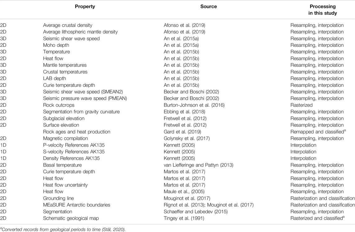
TABLE 1. Datasets used to populate the grid, in alphabetic order.
The 3D grid model and computational framework are intended for a wide range of applications, and are designed to be updated as additional data become available. Thus, we make constraints and related uncertainty from geology, geochronology and geophysics available in a form that is usable by researchers in geoscience, glaciology and ice sheet modeling. Through this contribution, we aim to facilitate interdisciplinary studies on the interaction between the solid Earth and cryosphere of Antarctica.
2. Data
Our model and framework includes numerous geological and geophysical datasets, together with the source reference, as listed in Table 1. We limit the spatial extent of the grid to the present coastline and ice shelf grounding line (Mouginot et al., 2017). Some processing, such as resampling and interpolation, is applied when the data are imported. Data in global projections are first reprojected, then interpolated to avoid artifacts and distortion when interpolating across the South Pole and anti-meridian line. Some of the datasets included in this contribution certainly contain spatial distortion due to reprojection. This distortion typically has its origin when published results are stored to a global grid. We do not aim to correct those artifacts in this contribution, as this would modify the datasets and require further discussion. Instead, we include the datasets as they are published.
Uncertainty information relating to each parameter is included where available (E.g., Martos et al., 2017). Those provided uncertainty values might not capture the total range of uncertainty that arise from necessary assumptions and resolution. Refined analysis of datasets and uncertainty can be achieved in the framework. However, this is beyond this contribution.
All data are also associated with provenance information and metadata that links the original source. Metadata are stored with the dataset in the grid. The agrid package (Stål and Reading, 2020) contains methods to access the data directly from the original sources, open online repositories and through Quantarctica (Roth et al., 2017). Links to web addresses, current at the time of writing, are provided in the Supplementary Material. In the case that a link becomes outdated, error handling is provided. There is no limitation to the number of datasets that can be included in a model. The datasets listed here are included to produce the test cases for appraisal of the framework.
3. Methods and Results
In this section we outline the methods used to construct the 3D grid and illustrate the functionality of the computational framework through usage examples. All computations in this study are performed using the Python package agrid (Stål and Reading, 2020). Use of agrid facilitates easy programming and compact scripts, with the underlying software being tailored to computations that use data, and metadata, held in the 3D grid. The figures in this study are generated using only a few lines of high level code, and functions provided with agrid. Where applicable, we utilize perceptually linear color representation (Crameri and Shephard, 2019; Morse et al., 2019).
3.1. Populating the 3D Grid
To populate the 3D model, the datasets listed in Table 1 are imported. Datasets are re-sampled and interpolated to the defined extent, resolution, projection and cell sizes. Here we use bi-linear interpolation, but other refined techniques are available. Data imported from polygon vectors are rasterized and attributes saved to the grid using a map function. Observations at point locations, such as geochronological data (compiled by Gard et al., 2019), are binned to the containing grid cells. Datasets are projected to WGS 84/Antarctic Polar Stereographic (EPSG:3031), with very limited distortion in continental Antarctica. The total grid extent is set to 6,200
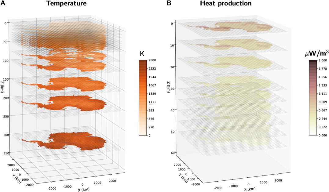
FIGURE 1. Oblique view of data held in the 3D grid model and illustration of plotting functionality. The model space is delineated by the Antarctic coastline and ice shelf grounding line (Mouginot et al., 2017). Depth sections are set to; 0, 8, 16, 25, 30, 35, 40, 45, 50, 75, 100, 150, 200, and 300 km. (A) Temperature in the crust and upper mantle derived from shear wavespeed by merging models AN1-Tc and AN1-Ts (An et al., 2015b) interpolated to defined grid. (B) Heat production in the crust from a simplified exponential function of depth, average production from age (Jaupart and Mareschal, 2013), segmentation by Schaeffer and Lebedev (2015) and crustal thickness from An et al. (2015a).
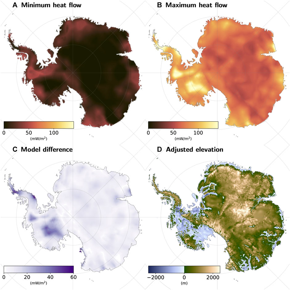
FIGURE 2. Examples of simple calculated outputs and visualisation in map view. Color representation is optimised for visibility. (A) Minimum subglacial heat flow from three studies (Maule et al., 2005; An et al., 2015b; Martos et al., 2017) using provided uncertainty ranges. (B) Maximum heat flow from the same three studies using provided uncertainty ranges. (C) Disagreement as standard deviation of the spread of the three studies. (D) Surface elevation with adjusted isostasy for ice removed. Calculated from Fretwell et al. (2012) and assuming constant density of ice 916.7 kg/m3, the crustal and mantle densities from Afonso et al. (2019). Moho from An et al. (2015a) and LAB from An et al. (2015b). A simple smoothing represents the rigidity of the lithosphere, as described in text.
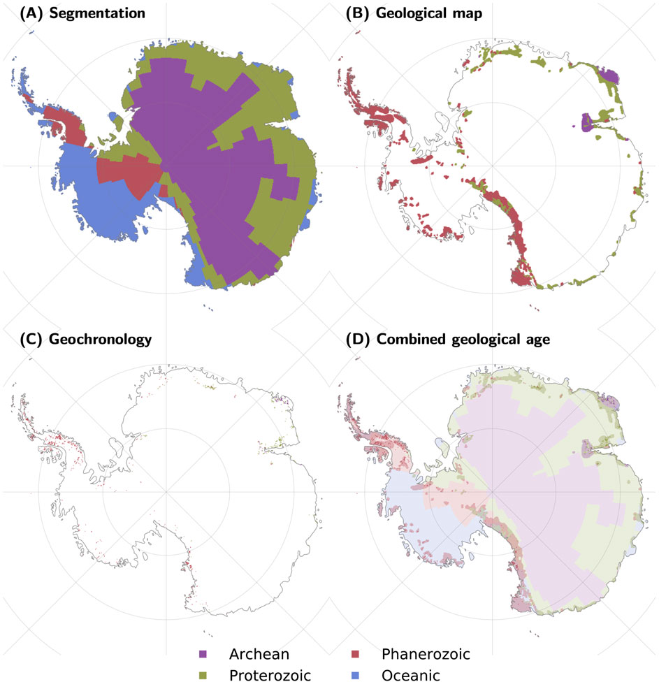
FIGURE 3. New maps generated to show the methodology of using data held in the 3D grid model. (A) Segmentation from seismic tomography (Schaeffer and Lebedev, 2015). (B) Schematic geological age map (Tingey et al., 1991). (C) Actual geochronology compiled by Gard et al. (2019). The dataset is clipped by mapped rock outcrops from Burton-Johnson and Riley (2015) to mitigate errors. (D) Geological age estimated from a combination of the previous three datasets, with Gard et al. (2019) as preferred and indicated with shading in a strong tone, Tingey et al. (1991) as midtone, and Schaeffer and Lebedev (2015) in faint tone. Continental crustal age, and geochronological data are divided into three classes (Janse, 1984) and as discussed in text: Archean (purple), Proterozoic (green) and Phanerozoic (brown). Suggested oceanic crust in Schaeffer and Lebedev (2015) is shown in blue. White indicates no data (B,C).
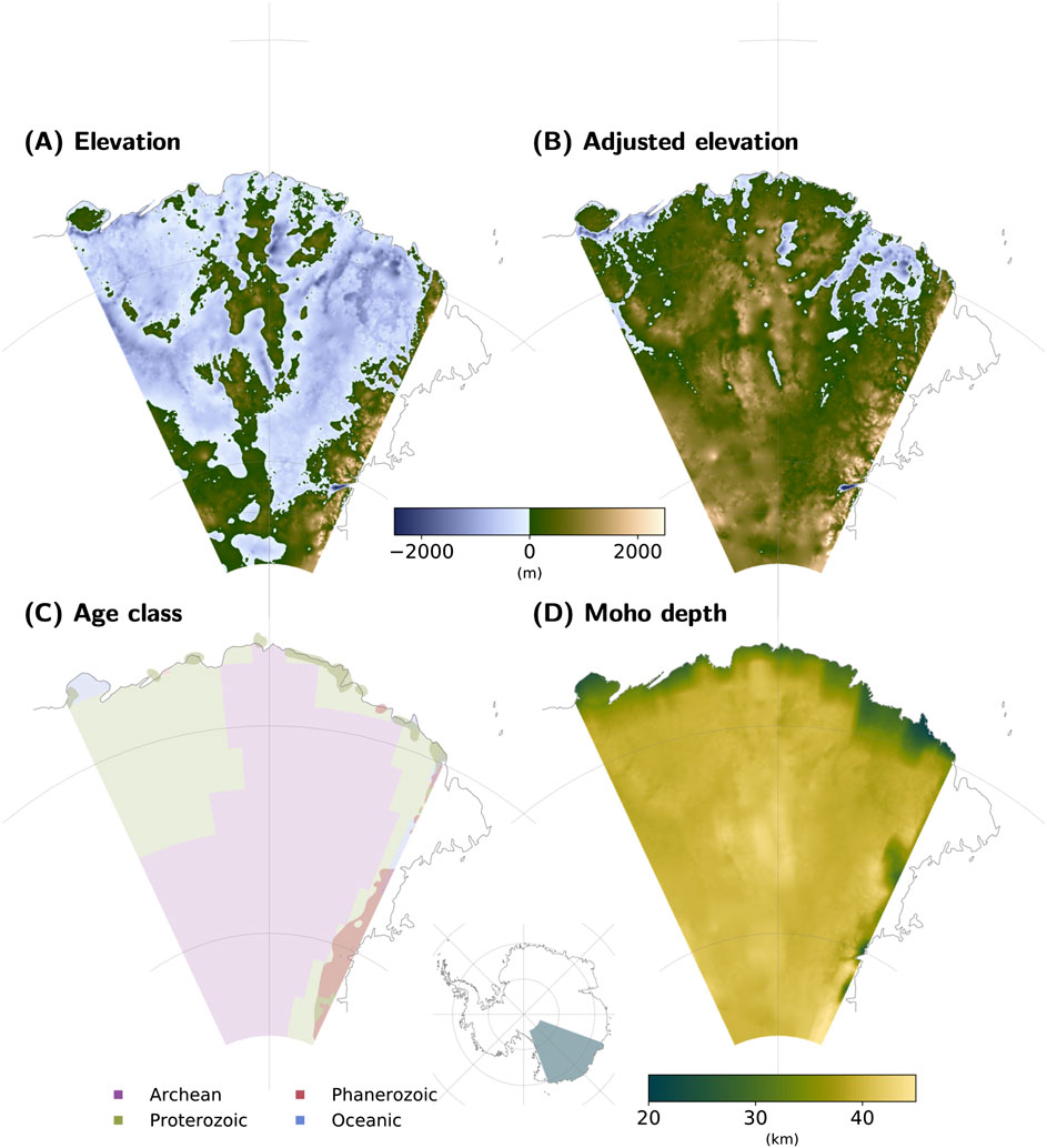
FIGURE 4. New maps generated for Wilkes Basin showing data held in the 3D grid model and calculated outputs at higher resolution. (A) Present subglacial topography, Bedmap2 (Fretwell et al., 2012). (B) Subglacial topography, with ice removed and isostasy corrected using crustal thickness from An et al. (2015a) and lithospheric thickness from An et al. (2015b). Crustal and upper mantle densities from Afonso et al. (2019). Bedrock elevation and surface elevation from Bedmap2 (Fretwell et al., 2012). (C) Estimates of crustal age. Cells with geological observations in strong tone (Burton-Johnson and Riley, 2015; Gard et al., 2019), schematic geology (Tingey et al., 1991) in mid tone, and segmentation from Schaeffer and Lebedev (2015) in light tone. Continental crustal age is classified into three classes, Archean (purple), Proterozoic (green), Phanerozoic (brown), together with oceanic crust (blue). Methods are discussed in the text. (D) Crustal thickness from An et al. (2015a).
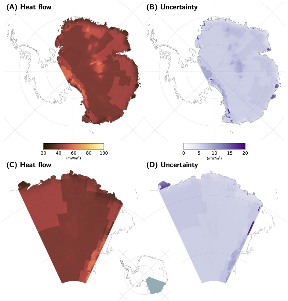
FIGURE 5. New maps generated by combining constraints from geophysical and geological data held in the 3D grid model: a new steady-state heat flow model, as discussed in text. (A) Heat flow map of East Antarctica, AqSS.ea (B) Uncertainty, as defined by the datasets used, excluding lateral uncertainties. (C) Heat flow map of Wilkes Basin, AqSS.wsb, (D) Uncertainty.
3.2. Computational Framework: Usage Examples
The agility of our 3D framework allows the rapid generation of maps or other outputs. Such products may be used to support research discussion or as numerical inputs for other studies (e.g., boundary conditions for ice sheet models).
3.2.1. Temperature in the Lithosphere and Heat Production in the Crust
Illustrating basic computation and oblique 3D visualisation using agrid and Antarctic datasets, Figure 1A shows lithospheric temperatures combined from AN-Ts and AN1-Tc (An et al., 2015b), interpolated to fit the grid. Figure 1B displays a first-order estimate of crustal heat production as a combination of crustal thickness (An et al., 2015a), segmentation (Schaeffer and Lebedev, 2015), heat production estimate from crustal age (Jaupart et al., 2016) and decreasing heat production as an exponential function of depth:
where A is the value of heat production in W/m3,
3.2.2. Calculated Outputs Based on Multiple Geophysical Datasets
Illustrating further examples of computation and visualisation in map view, Figure 2 shows constraints from multiple heat flow models, and adjusted surface elevation based on multiple datasets. Minimum heat flow (Figure 2A) and maximum heat flow (Figure 2B) are the lowest and highest values at each grid cell in any of Maule et al. (2005), An et al. (2015b), and Martos et al. (2017), including provided uncertainty. Figure 2C shows the standard deviation as a measure of disagreement between the heat flow maps from aforementioned studies. Areas are readily seen where ice sheet modellers should be particularly careful when using the geothermal heat contribution as a boundary condition. The property maps shown in Figures 2A–C could therefore be useful for sensitivity studies of the impact of geothermal heat on the ice sheet at a continental scale.
Isostatic models are used to understand how the Antarctic crust and upper mantle interact with the cryosphere (e.g., O’Donnell and Nyblade, 2014). Figures 2D, 4B show bedrock elevation for isostatically relaxed ice-free conditions. Such computations are easy to perform in our framework, for example, using the simplified formula:
where
3.2.3. Mapping Crustal Age by Merging Geological and Geophysical Datasets
Mapping crustal age provides an illustration of merging geological and geophysical sources, addressing the challenge of combining categorical and numerical data types. We utilize geochronological measurements compiled by Gard et al. (2019). The number of samples (Supplementary Material), mode, average value and standard deviation are calculated and binned to each cell. The legacy schematic geology map from Tingey et al. (1991) is used for reference and to guide moderate extrapolation of geology. Age estimates expressed in geological time are converted to age in years (Stål, 2020). Where no geological observations or extrapolation are available, we use crustal segmentation informed by seismic tomography. Most global regionalization studies often exclude or oversimplify Antarctica due to the limited available data (e.g., Jordan, 1981; Artemieva and Mooney, 2001; Artemieva, 2006; Artemieva, 2009). We implement one of the few continental scale segmentation models that covers Antarctica, the k-means clustering of surface-wave dispersion from Schaeffer and Lebedev (2015), which makes use of methods by Lekić et al. (2010) and data first presented by Schaeffer and Lebedev (2013). Examples of the standardised content reduced to three age classes and oceanic crust are shown on a continental (Figure 3) and regional scale (Figure 4C). The shading tone indicates the source, and hence, the robustness of the constraint. Direct observations (Gard et al., 2019) are strong in tone, schematic geological domains (Tingey et al., 1991) are shown in midtone and geophysical regionalisation (Schaeffer and Lebedev, 2015) is shaded in a faint tone. Combining data of different types is straightforward in concept, but challenging in practice, and the new framework shows that this can be achieved in a repeatable manner.
3.2.4. Calculated Outputs at Higher Resolution
Illustrating the functionality of the 3D model and framework at a regional scale, Figure 4 shows data held in the 3D grid and calculated outputs for the Wilkes Subglacial Basin. Figure 4A is a representation of the Bedmap2 dataset (Fretwell et al., 2012). Figure 4B shows the same simplified isostatic correction as Figure 2D in higher resolution. Figure 4C shows the combined model of crustal stabilisation age, using same methods as for Figure 3D, again at higher resolution, for the Wilkes Basin.
3.2.5. AqSS, a Steady-State Heat Flow Model
We further illustrate the functionality of the computational framework through generating a Steady-state heat flow model, AqSS, which combines geophysical and geological data. steady-state models can be reduced to two components that are identified as sources of geothermal heat: heat from the Earth’s core and mantle, reaching the crust as heat flow through the Moho,
where
From studies in different geological settings and methods, the mantle component has been constrained to
Uncertainty for AqSS is calculated from the uncertainty provided with each dataset, assuming they are independent.
where
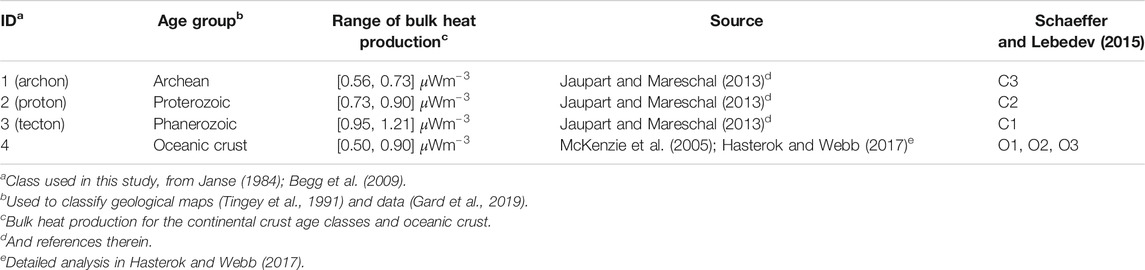
TABLE 2. Thermal properties assigned to crustal domains.
By assuming steady-state conditions throughout East Antarctica and applying a constant contribution from the mantle (Mareschal and Jaupart, 2004), we avoid invoking any assumptions regarding temperatures in the lower crust or upper mantle. The larger part of the total heat flow is heterogeneous and originates from the crust (e.g., Jaupart et al., 2016; Burton-Johnson et al., 2017). To assign crustal heat production (A), we use the geological observations and crustal segmentation, as described in the previous section. We divide the crust into three classes according to stabilisation age: Archean-Paleoproterozoic, Meso-Neoproterozoic and Phanerozoic (Janse, 1984; Begg et al., 2009; Jaupart and Mareschal, 2013; Jaupart et al., 2016). For each class, an average heat production range is applied from Jaupart and Mareschal (2013). Crustal thickness is constrained from seismology (An et al., 2015a) and shown in Figure 4D. Details of the classification are given in Table 2.
We use the segmentation in Figures 3D, 4C to calculate new heat flow maps based on geophysical and geological input data using the methods described in the previous section. The resulting steady-state heat flow and associated uncertainties for the approach used, are shown in Figure 5. This provides an illustration of the further ability to compute output based on data of different types. Figure 5A shows our new mapped heat flow estimate, AqSS.ea, at continental scale. Figure 5C shows a regional equivalent for the Wilkes Subglacial Basin, AqSS.wsb, as an illustration of working at higher resolution. Calculated uncertainties are shown in Figure 5B, for East Antarctica, and Figure 5D for Wilkes Subglacial Basin.
3.2.6. Appraisal of the Steady-State Heat Flow Model, AqSS, and Previous Models
Our final set of functionality examples illustrate using the framework to appraise alternate models for a given parameter. Figure 6A compares AqSS, minimum and maximum values, with earlier published models and calculated heat flow from borehole measurements in western part of Australia (compiled by Hasterok, 2019). The Australian dataset includes transient and shallow processes, that are not captured in AqSS nor some of the other geophysically derived estimates.
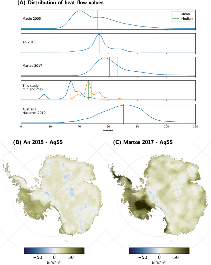
FIGURE 6. Comparison of heat flow models enabled by the 3D model and framework. (A) Distribution of heat flow values. For East Antarctica, distributions from Fox Maule et al. (2005), An et al. (2015b), Martos et al. (2017), example heat flow values for AqSS (derived from values mapped in Figures 5A,B) as minimum estimate (blue line) and maximum estimate (red line); for Australia, distribution of actual measurements in southern and western Australia compiled by Hasterok (2019). (B) Heat flow model from seismic data (An et al., 2015b) minus AqSS. (C) Heat flow model from magnetic data (Martos et al., 2017) minus AqSS. Subtracting AqSS, which is a steady-state heat flow model, from published maps of total heat flow indicates non-steady-state contributions to total heat flow.
Figures 6B,C show examples of comparing two observation-derived datasets with a constructed reference model to inform the discussion of lithospheric properties. We show An et al. (2015b) and Martos et al. (2017) heat flow maps minus steady-state heat flow from AqSS. These two alternative results are effectively the additional heat flow likely generated from neotectonic and other non steady-state processes, such as recent rifting, volcanism and orogenesis.
3.2.7. Variation of Thermal Gradients With Depth
Figure 7 illustrates an example of extracting the variation of a property with depth. We show thermal gradients from locations in West and East Antarctica as a Gaussian kernel density estimate (KDE), including seismic-derived temperatures (An et al., 2015b) and magnetic-derived Curie temperature depth, including uncertainty bounds (Martos et al., 2017). The KDE is calculated over the depth dimension for East and West Antarctica separately. We also include uncertainties when defining the kernel size. In West Antarctica, the example is from Lake Whillans, the location of one of few direct measurements of heat flow in Antarctica (Fisher et al., 2015). In East Antarctica, the example is from Dome C. The location maps, showing West and East Antarctica, are obtained by importing a polygon vector to use as a factor (inset in Figures 7A,B).
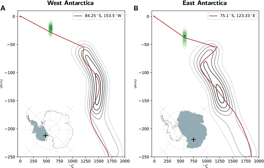
FIGURE 7. Illustration of framework capability to extract depth profiles for model comparison. Thermal model of the lithosphere, populated with data from Antarctic heat flow models for West and East Antarctica reduced to kernel density estimations (KDE). Temperatures derived from seismic data, An et al. (2015b), in black contours showing highest concentration of thermal profiles. Depth to Curie temperature isotherm with uncertainty derived from magnetic data (Martos et al., 2017) in green contours. Surface and subglacial elevation from Fretwell et al. (2012) and subglacial temperature from van Liefferinge et al. (2018) in red at the surface. KDE Gaussian kernel for mantle temperatures set to 100°C/10 km, for Curie temperature isotherm 25°C/2 km and for surface 5°C/0.1 km. Plotted profiles in red show two examples locations of 1D temperature models using combined input. The subglacial heat flow is proportional to the gradient of temperature and the thermal conductivity in the upper crust. To facilitate KDE, only every fifth grid cell is computed. The figure is cropped at 250 km depth. Insets show sampled area.
The contours show the range of allowed values and how the two models, An et al. (2015b) and Martos et al. (2017), compare in depth section. The profile of temperature with depth varies over a large range for both example locations (Figure 7 red line), and when an average kernel is displayed (Figure 7 gray contours). This result, and the use of the 3D grid and framework in comparing models and sensitivity to different parameters, is further discussed below.
4. Discussion
We first outline the most significant limitations of the 3D model and framework, and then discuss aspects of our newly generated heat flow example, as an exemplar of how the research environment might be used.
4.1. Limitations
There is a trade-off between resolution and computational expense for any numerical model. Moreover, numerical stability is, in general, required for grid-based calculations. The continental scale model in 20
The model functionality allows for the inclusion of uncertainty values matching each dataset. Therefore, the impact of the noted limitations can be mitigated. The model can be realized with a desired extent, resolution and data content to suit the needed outcome and stage of research. In this contribution, we include the uncertainties provided with the datasets. Those metrics may not cover the true uncertainty of the datasets, when resolution and artifacts from the methodology are considered. The strength of the framework is that the impact of such concerns can be understood as data coverage improves.
4.2. Insight From Examples
The heat flow estimate exemplifies how our multidimensional and multivariate grid may be used to combine input data of different types, and execute calculations across the grid. This provides, we hope, a constructive approach to reconcile the differences between published heat flow models for Antarctica (Figure 2C).
The comparison of the results from magnetic and seismic studies provides new insight into deep Earth properties since both approaches estimate temperature gradients, but using different methods. The differences in Curie temperature depths from seismic (An et al., 2015b) and magnetic (Martos et al., 2017) studies are larger in East Antarctica than in West Antarctica (Supplementary Material). These observations imply properties of the lithosphere such as fluid content and heterogeneous heat production that are not captured in the methods used. Compositional variations and presence of fluids impact the seismic wave speed and hence estimated temperatures (Hirth and Kohlstedt, 1996; Goes et al., 2000; Haeger et al., 2019). Magnetic models depend on a simplified crustal thermal and magnetic structure. As an example of a departure from the assumed case, shallow felsic intrusions can provide a large contribution to the surface heat flow, and this could be observed as a deeper Curie temperature isotherm because removal of radiogenic heat producing material facilitates cooling of the lower crust (Jaupart et al., 2016). Figure 7 highlights the large range and uncertainties involved in present heat flow estimates and also illustrates the much steeper thermal gradient in the crust compared to the upper mantle. We note that thermal conductivity generally decreases with temperature (Xu et al., 2004; McKenzie et al., 2005). However, geothermal heat is not lost rapidly through the crust, so crustal heat production must have a large influence on geothermal heat flow at the surface. New outputs such as Figure 7 show how the limitations in available evidence give rise to temperature changes with depth in the upper mantle that are, taken together, implausible. For example, a temperature decrease with depth is highly unlikely in stable lithosphere. The valuable studies that we have compared note their underlying assumptions and logical simplifications. Our new model and framework allows the implications of such simplifications to be better understood.
We have introduced a new conceptual heat flow model, AqSS, where we base the calculations on the energy balance of the lithosphere, rather than estimated temperature gradients. Our method represents a new approach in the Antarctic context and and uses a reduced number of assumptions. With negligible heat generated in the lithospheric mantle (An et al., 2015b; Jaupart et al., 2016; Martos et al., 2017), the Moho steady-state heat flux must be equal to the flux at the lithosphere-asthenosphere boundary. For old and stable crust, the mantle component of the heat can be reduced to a low and constant value in the range between 10–20
4.3. Use Cases for the 3D Model and Software Framework
The main use cases for Antarctic research, with an emphasis on interdisciplinary studies of the interaction of the solid Earth and cryosphere, are listed below:
(1) Computing results based on geophysical datasets. A broad range of datasets can be combined in the same frame and uncertainty bounds included, as illustrated in this contribution. The extensive toolboxes from, e.g., the Python ecosystem are available for modeling and analysis. Import, export and visualisation functions simplify the workflow. Supplementary Figure S4 shows the potential for experimentation in data visualisation.
(2) Combining geophysics and geological constraints, and making use of the merged result in ongoing calculations, as illustrated in this contribution. Constraints from glaciology could potentially be included in the same way, e.g., as a constraint on shallow processes to facilitate discussion of heat flow estimates for given regions.
(3) Appraisal of models. Comparisons between datasets, or calculated differences, can provide insights that are beyond the potential of the individual contributing studies, again, as we have illustrated in this contribution.
(4) Working with uncertainty and probabilistic methods. With the large uncertainties involved in Antarctic solid Earth research, probabilistic tools are essential to progress in the understanding of the Antarctic lithosphere. A productive way forward is to embrace the uncertainties and build probabilistic models (e.g., Stål et al., 2019). The computational framework that is presented here is well-suited to this task and provides an environment where data and associated uncertainties, probabilities and likelihoods can be processed.
(5) An enabling capability for the international research community. Building robust models of the Antarctic crust and upper mantle is a community effort, that will be refined incrementally with additional data. When a specific research product is desired, e.g., a reference heat flow map to include in ice sheet models, we can now draw constraints from multiple studies and/or easily test a range of alternative maps.
5. Conclusions
We present a new 3D grid model and framework: a computing environment tailored to interdisciplinary research. The software framework is easy to use, allows geophysical and geological data to be combined, and provides a virtual laboratory to develop and test, for example, solid Earth models. The model points directly to published data sources and the data contained can easily be updated.
This contribution aims to facilitate progress in Antarctic research concerning solid Earth-cryosphere interaction. Physical property maps and grids, of utility to studies of glacial isostatic adjustment, geothermal heat and the shaping of topography can be performed; bridging between the solid Earth and cryosphere research communities. The usage examples that we provide include a conceptually new steady-state heat flow map based on the energy balance of the lithosphere for comparison with maps based on modeled thermal gradient.
Data Availability Statement
Publicly available datasets were analyzed in this study. This data can be found here: Code and output products to be made available from Pangea: https://doi.pangaea.de/10.1594/PANGAEA.918549. Code includes updated URL to all used datasets. Code also published on Zenodo: https://doi.org/10.5281/zenodo.3775166.
Author Contributions
TS developed the software, built the 3D model, generated the examples and wrote the first draft text. AR guided the overarching research direction and advised on the geophysics. JH advised on the geology. SP advised on the interdisciplinary context. JW advised on the plate tectonics and basin geoscience. All authors contributed to revising the text.
Funding
This research was supported under Australian Research Council’s Special Research Initiative for Antarctic Gateway Partnership (Project ID SR140300001) and the Center for Southern Hemisphere Oceans Research, a joint research center between QNLM and CSIRO.
Conflict of Interest
The authors declare that the research was conducted in the absence of any commercial or financial relationships that could be construed as a potential conflict of interest.
Acknowledgments
This research is a contribution to the SCAR SERCE program.
Supplementary Material
The Supplementary Material for this article can be found online at: https://www.frontiersin.org/articles/10.3389/feart.2020.577502/full#supplementary-material
References
Adie, R. J., and Adie, R. J. (1977). Earth sciences: the geology of Antarctica: a review. Philos. Trans. R. Soc. Lond. B Biol. Sci. 279, 123–130. doi:10.1098/rstb.1977.0077
Afonso, J. C., Salajegheh, F., Szwillus, W., Ebbing, J., and Gaina, C. (2019). A global reference model of the lithosphere and upper mantle from joint inversion and analysis of multiple data sets. Geophys. J. Int. 217, 1602–1628. doi:10.1093/gji/ggz094
Aitken, A. R. A., Young, D. A., Ferraccioli, F., Betts, P. G., Greenbaum, J. S., Richter, T. G., et al. (2014). The subglacial geology of Wilkes Land, East Antarctica. Geophys. Res. Lett. 41, 2390–2400. doi:10.1002/2014GL059405
An, M., and Shi, Y. (2007). Three-dimensional thermal structure of the Chinese continental crust and upper mantle. Sci. China, Ser. A D 50, 1441–1451. doi:10.1007/s11430-007-0071-3
An, M., Wiens, D. A., Zhao, Y., Feng, M., Nyblade, A. A., Kanao, M., et al. (2015a). S -velocity model and inferred Moho topography beneath the Antarctic plate from Rayleigh waves. J. Geophys. Res. Solid Earth 120, 359–383. doi:10.1002/2014JB011332
An, M., Wiens, D. A., Zhao, Y., Feng, M., Nyblade, A., Kanao, M., et al. (2015b). Temperature, lithosphere-asthenosphere boundary, and heat flux beneath the Antarctic Plate inferred from seismic velocities. J. Geophys. Res. Solid Earth 120, 8720–8742. doi:10.1002/2015JB011917
Artemieva, I. M. (2006). Global 1°×1° thermal model TC1 for the continental lithosphere: implications for lithosphere secular evolution. Tectonophysics 416, 245–277. doi:10.1016/j.tecto.2005.11.022
Artemieva, I. M., and Mooney, W. D. (2001). Thermal thickness and evolution of Precambrian lithosphere: a global study. J. Geophys. Res. 106, 16387–16414. doi:10.1029/2000jb900439
Artemieva, I. (2011). The Lithosphere: an interdisciplinary approach. Cambridge, England: Cambridge University Press.
Artemieva, I. M. (2009). The continental lithosphere: reconciling thermal, seismic, and petrologic data. Lithos 109, 23–46. doi:10.1016/j.lithos.2008.09.015
Artemieva, I. M., and Thybo, H. (2020). Continent size revisited: geophysical evidence for West Antarctica as a back-arc system. Earth Sci. Rev. 202, 103106. doi:10.1016/j.earscirev.2020.103106
Baranov, A., Tenzer, R., and Bagherbandi, M. (2018). Combined gravimetric-seismic crustal model for Antarctica. Surv. Geophys. 39, 23–56. doi:10.1007/s10712-017-9423-5
Beardsmore, G. R., and Cull, J. P. (2001). Crustal heat flow. Cambridge, England: Cambridge University Press.Google Scholar
Becker, T. W., and Boschi, L. (2002). A comparison of tomographic and geodynamic mantle models. Geochemistry Geophysics Geosystems 3. doi:10.1029/2001gc000168
Begeman, C. B., Tulaczyk, S. M., and Fisher, A. T. (2017). Spatially variable geothermal heat flux in west Antarctica: evidence and implications. Geophys. Res. Lett. 44, 9823–9832. doi:10.1002/2017GL075579
Begg, G. C., Griffin, W. L., Natapov, L. M., O’Reilly, S. Y., Grand, S. P., O’Neill, C. J., et al. (2009). The lithospheric architecture of Africa: seismic tomography, mantle petrology, and tectonic evolution. Geosphere 5, 23–50. doi:10.1130/GES00179.1
Boger, S. D. (2011). Antarctica - before and after Gondwana. Gondwana Res. 19, 335–371. doi:10.1016/j.gr.2010.09.003
Burton-Johnson, A., Black, M., Fretwell, P. T., and Kaluza-Gilbert, J. (2016). An automated methodology for differentiating rock from snow, clouds and sea in Antarctica from Landsat 8 imagery: a new rock outcrop map and area estimation for the entire Antarctic continent. Cryosphere 10, 1665–1677. doi:10.5194/tc-10-1665-2016
Burton-Johnson, A., Dziadek, R., and Martin, C. (2020). Geothermal heat flow in Antarctica: current and future directions. Cryosphere Discuss. doi:10.5194/tc-2020-59
Burton-Johnson, A., Halpin, J. A., Whittaker, J. M., Graham, F. S., and Watson, S. J. (2017). A new heat flux model for the Antarctic Peninsula incorporating spatially variable upper crustal radiogenic heat production. Geophys. Res. Lett. 44, 5436–5446. doi:10.1002/2017GL073596
Burton-Johnson, A., and Riley, T. R. (2015). Autochthonous v. Accreted Terrane development of continental margins: a revised in situ tectonic history of the Antarctic Peninsula. J. Geol. Soc. 172, 822–835. doi:10.1144/jgs2014-110
Cammarano, F., Goes, S., Vacher, P., and Giardini, D. (2003). Inferring upper-mantle temperatures from seismic velocities. Phys. Earth Planet. In. 138, 197–222. doi:10.1016/S0031-9201(03)00156-0
Carson, C. J., McLaren, S., Roberts, J. L., Boger, S. D., and Blankenship, D. D. (2014). Hot rocks in a cold place: high sub-glacial heat flow in East Antarctica. J. Geol. Soc. 171, 9–12. doi:10.1144/jgs2013-030
Chen, B., Haeger, C., Kaban, M. K., and Petrunin, A. G. (2018). Variations of the effective elastic thickness reveal tectonic fragmentation of the Antarctic lithosphere. Tectonophysics 746, 412–424. doi:10.1016/j.tecto.2017.06.012
Christensen, N. I. (1988). The continental crust: a geophysical approach. Cambridge, MA: Academic Press, Vol. 69. doi:10.1029/88eo00170
Corvino, A. F., Boger, S. D., Henjes-Kunst, F., Wilson, C. J. L., and Fitzsimons, I. C. W. (2008). Superimposed tectonic events at 2450Ma, 2100Ma, 900Ma and 500Ma in the north mawson escarpment, Antarctic Prince Charles Mountains. Precambrian Res. 167, 281–302. doi:10.1016/j.precamres.2008.09.001
Cowton, T., Nienow, P., Bartholomew, I., Sole, A., and Mair, D. (2012). Rapid erosion beneath the Greenland ice sheet. Geology 40, 343–346. doi:10.1130/G32687.1
Cox, S. C., Smith-Lyttle, B., Siddoway, C., Capponi, G., Elvevold, S., Burton-Johnson, A., et al. (2018). The GeoMAP dataset of Antarctic rock exposures. In Polar2018, Davos: SCAR March 6, 2019.
Craddock, C. (1970). Antarctic geology and gondwanaland. Bull. At. Sci. 26, 33–39. doi:10.1080/00963402.1970.11457870
Crameri, F., and Shephard, G. E. (2019). Scientific Colour Maps. (Version 5.0.0). Zenodo. doi:10.5281/zenodo.3596401
Cull, J. P. (1982). An appraisal of Australian heat-flow data. BMR (Bur. Miner. Resour.) J. Aust. Geol. Geophys. 7. 11–21.
Daczko, N. R., Halpin, J. A., Fitzsimons, I. C. W., and Whittaker, J. M. (2018). A cryptic Gondwana-forming orogen located in Antarctica. Sci. Rep. 8, 1–9. doi:10.1038/s41598-018-26530-1
DeConto, R. M., and Pollard, D. (2016). Contribution of Antarctica to past and future sea-level rise. Nature 531, 591–597. doi:10.1038/nature17145
Dinniman, M., Asay-Davis, X. S., Asay-Davis, X., Galton-Fenzi, B., Holland, P., Jenkins, A., et al. (2016). Modeling ice shelf/ocean interaction in Antarctica: a review. Oceanog. 29, 144–153. doi:10.5670/oceanog.2016.106
Divincenzo, G., Talarico, F., and Kleinschmidt, G. (2007). An 40Ar-39Ar investigation of the Mertz Glacier area (George V Land, Antarctica): implications for the ross orogen-East Antarctic craton relationship and gondwana reconstructions. Precambrian Res. 152, 93–118. doi:10.1016/j.precamres.2006.10.002
Du Toit, A. L. (1937). Our wandering continents: an hypothesis of continental drifting: “Africa forms the key”. London, UK: Oliver & Boyd.
Ebbing, J., Haas, P., Ferraccioli, F., Pappa, F., Szwillus, W., and Bouman, J. (2018). Earth tectonics as seen by GOCE - enhanced satellite gravity gradient imaging. Sci. Rep. 8, 1–9. doi:10.1038/s41598-018-34733-9
Ferraccioli, F., Finn, C. A., Jordan, T. A., Bell, R. E., Anderson, L. M., and Damaske, D. (2011). East Antarctic rifting triggers uplift of the Gamburtsev Mountains. Nature 479, 388–392. doi:10.1038/nature10566
Fisher, A. T., Mankoff, K. D., Tulaczyk, S. M., Tyler, S. W., and Foley, N. (2015). High geothermal heat flux measured below the West Antarctic ice sheet. Sci. Adv. 1, e1500093–e1500099. doi:10.1126/sciadv.1500093
Fitzsimons, I. C. W. (2000). A review of tectonic events in the East Antarctic shield and their implications for Gondwana and earlier supercontinents. J. Afr. Earth Sci. 31, 3–23. doi:10.1016/S0899-5362(00)00069-5
Forsberg, R., Olesen, A. V., Ferraccioli, F., Jordan, T., Corrand, H., and Matsuoka, K. (2017). PolarGap 2015/16 Filling the GOCE polar gap in Antarctica and ASIRAS flight around South Pole. Tech. rep., DTU-space, BAS, NPI
Boger, S. D. (2011). Antarctica - before and after gondwana. Gondwana Res. 19, 335–371. doi:10.1016/j.gr.2010.09.003
Förste, C., Bruinsma, S., Flechtner, F., Marty, J.-C., Dahle, C., Abrykosov, O., et al. (2013). EIGEN-6C2-A new combined global gravity field model including GOCE data up to degree and order 1949 of GFZ Potsdam and GRGS Toulouse. EGU General Assembly Conference Abstracts, 15, 4077.
Fowler, C. M. (1990). The solid earth: an introduction to global geophysics Cambridge, England: Cambridge University Press. doi:10.1029/90eo00309
Fretwell, P., Pritchard, H. D., Vaughan, D. G., Bamber, J. L., Barrand, N. E., Bell, R., et al. (2012). Bedmap2: improved ice bed, surface and thickness datasets for Antarctica. Cryosphere Discuss. 6, 4305–4361. doi:10.5194/tcd-6-4305-2012
Frieler, K., Clark, P. U., He, F., Buizert, C., Reese, R., Ligtenberg, S. R. M., et al. (2015). Consistent evidence of increasing Antarctic accumulation with warming. Nat. Clim. Change 5, 348–352. doi:10.1038/nclimate2574
Gard, M., Hasterok, D., and Halpin, J. A. (2019). Global whole-rock geochemical database compilation. Earth Syst. Sci. Data 11, 1553–1566. doi:10.5194/essd-11-1553-2019
Goes, S., Govers, R., and Vacher, P. (2000). Shallow mantle temperatures under Europe from P and S wave tomography. J. Geophys. Res. 105, 11153–11169. doi:10.1029/1999jb900300
Goff, J. A., Powell, E. M., Young, D. A., and Blankenship, D. D. (2014). Conditional simulation of Thwaites Glacier (Antarctica) bed topography for flow models: incorporating inhomogeneous statistics and channelized morphology. J. Glaciol. 60, 635–646. doi:10.3189/2014JoG13J200
Golledge, N. R., Keller, E. D., Gomez, N., Naughten, K. A., Bernales, J., Trusel, L. D., et al. (2019). Global environmental consequences of twenty-first-century ice-sheet melt. Nature 566, 65–72. doi:10.1038/s41586-019-0889-9
Golledge, N. R., Kowalewski, D. E., Naish, T. R., Levy, R. H., Fogwill, C. J., and Gasson, E. G. W. (2015). The multi-millennial Antarctic commitment to future sea-level rise. Nature 526, 421–425. doi:10.1038/nature15706
Golynsky, A., Bell, R., Blankenship, D., Damaske, D., Ferraccioli, F., Finn, C., et al. (2013). Air and shipborne magnetic surveys of the Antarctic into the 21st century. Tectonophysics 585, 3–12. doi:10.1016/j.tecto.2012.02.017
Golynsky, A. V., Golynsky, D. A., Ferraccioli, F., Jordan, T. A., Blankenship, D. D., Holt, J., et al. (2017). ADMAP-2: magnetic anomaly map of the Antarctic, 1:10 000 000 scale map. Incheon South Korea: Korea Polar Research Institute. doi:10.22663/ADMAP.V2 [Dataset].
Goodge, J. W., and Finn, C. A. (2010). Glimpses of East Antarctica: aeromagnetic and satellite magnetic view from the central Transantarctic Mountains of East Antarctica. J. Geophys. Res. 115, 1–22. doi:10.1029/2009JB006890
Goodge, J. W., Hansen, V. L., and Peacock, S. M. (1992). Multiple petrotectonic events in high-grade metamorphic rocks of the Nimrod Group, central Transantarctic Mountains, Antarctica. Recent Progress in Antarctic Earth Science. 203–209.
Graham, F. S., Roberts, J. L., Galton-Fenzi, B. K., Young, D., Blankenship, D., and Siegert, M. J. (2017). A high-resolution synthetic bed elevation grid of the Antarctic continent. Earth Syst. Sci. Data 9, 267–279. doi:10.5194/essd-9-267-2017
Greenbaum, J. S., Blankenship, D. D., Young, D. A., Richter, T. G., Roberts, J. L., Aitken, A. R. A., et al. (2015). Ocean access to a cavity beneath totten glacier in East Antarctica. Nat. Geosci. 8, 294–298. doi:10.1038/ngeo2388
Guillou, L., Mareschal, J.-C., Jaupart, C., Gariépy, C., Bienfait, G., and Lapointe, R. (1994). Heat flow, gravity and structure of the Abitibi belt, Superior Province, Canada: implications for mantle heat flow. Earth Planet Sci. Lett. 122, 103–123. doi:10.1016/0012-821X(94)90054-X
Gunter, B. C., Didova, O., Riva, R. E. M., Ligtenberg, S. R. M., Lenaerts, J. T. M., King, M. A., et al. (2014). Empirical estimation of present-day Antarctic glacial isostatic adjustment and ice mass change. Cryosphere 8, 743–760. doi:10.5194/tc-8-743-2014
Haeger, C., Kaban, M. K., Tesauro, M., Petrunin, A. G., and Mooney, W. D. (2019). 3-D density, thermal, and compositional model of the Antarctic lithosphere and implications for its evolution. G-cubed 20, 688–707. doi:10.1029/2018GC008033
Halpin, J. A., Daczko, N. R., Milan, L. A., and Clarke, G. L. (2012). Decoding near-concordant U-Pb zircon ages spanning several hundred million years: recrystallisation, metamictisation or diffusion? Contrib. Mineral. Petrol. 163, 67–85. doi:10.1007/s00410-011-0659-7
Halpin, J. A., Gerakiteys, C. L., Clarke, G. L., Belousova, E. A., and Griffin, W. L. (2005). In-situ U-Pb geochronology and Hf isotope analyses of the Rayner Complex, east Antarctica. Contrib. Mineral. Petrol. 148, 689–706. doi:10.1007/s00410-004-0627-6
Hansen, S. E., Kenyon, L. M., Graw, J. H., Park, Y., and Nyblade, A. A. (2016). Crustal structure beneath the northern Transantarctic Mountains and Wilkes Subglacial Basin: implications for tectonic origins. J. Geophys. Res. Solid Earth 121, 812–825. doi:10.1002/2015JB012325
Hansen, S. E., Nyblade, A. A., Heeszel, D. S., Wiens, D. A., Shore, P., and Kanao, M. (2010). Crustal structure of the Gamburtsev Mountains, East Antarctica, from S-wave receiver functions and Rayleigh wave phase velocities. Earth Planet Sci. Lett. 300, 395–401. doi:10.1016/j.epsl.2010.10.022
Harley, S. L., Fitzsimons, I. C. W., and Zhao, Y. (2013). Antarctica and supercontinent evolution: historical perspectives, recent advances and unresolved issues, Geological Society, London, Special Publications. 383, 1–34. doi:10.1144/SP383.9
Harris, C. R., Millman, K. J., van der Walt, S. J., Gommers, R., Virtanen, P., Cournapeau, D., et al. (2020). Array programming with NumPy., Nature, 585, (7825) 357–362. doi:10.1038/s41586-020-2649-2
Hasterok, D. (2019). Thermoglobe. www.heatflow.org [Dataset].
Hasterok, D., and Webb, J. (2017). On the radiogenic heat production of igneous rocks. Geosci. Front. 8, 919–940. doi:10.1016/j.gsf.2017.03.006
Heeszel, D. S., Wiens, D. A., Anandakrishnan, S., Aster, R. C., Dalziel, I. W. D., Huerta, A. D., et al. (2016). Upper mantle structure of central and West Antarctica from array analysis of Rayleigh wave phase velocities. J. Geophys. Res. Solid Earth 121, 1758–1775. doi:10.1002/2015JB012616
Hirth, G., and Kohlstedt, D. L. (1996). Water in the oceanic upper mantle: implications for rheology, melt extraction and the evolution of the lithosphere. Earth Planet Sci. Lett. 144, 93–108. doi:10.1016/0012-821x(96)00154-9
Hoyer, S., and Hamman, J. J. (2017). xarray: N-D labeled Arrays and Datasets in Python. J. Open Res. Software 5, 1–6. doi:10.5334/jors.148
Jacobs, J., Elburg, M., Läufer, A., Kleinhanns, I. C., Henjes-Kunst, F., Estrada, S., et al. (2015). Two distinct late mesoproterozoic/early neoproterozoic basement provinces in central/eastern dronning Maud Land, East Antarctica: the missing link, 15-21°E. Precambrian Res. 265, 249–272. doi:10.1016/j.precamres.2015.05.003
Jacobs, J., Fanning, C. M., Henjes-Kunst, F., Olesch, M., and Paech, H. J. (1998). Continuation of the Mozambique belt into east Antarctica: Grenville‐age metamorphism and polyphase Pan‐African high‐grade events in central dronning Maud Land. J. Geol. 106, 385–406. doi:10.1086/516031
Jamieson, S. S. R., and Sugden, D. E. (2008). Landscape evolution of Antarctica. In and the 10th I. editorial team Alan K. CAlan K. Cooper, Peter Barrett, Howard Stagg, Bryan Storey, Edmund Stump, Woody Wise, and the 10th ISAES editorial teamooper, Peter Barrett, Howard Stagg, Bryan Storey, Edmund Stump, Woody Wise (Ed.), Antarctica: A Keystone in a Changing World Proceedings of the 10th International Symposium on Antarctic Earth Sciences, Santa Barbara, California, August 26 to September 1, 2007 (Issue June 2014, pp. 39‐54). Polar Research Board, National Research Council, U.S. Geological. doi:10.3133/of2007-1047.kp05
Jamieson, S. S. R., Sugden, D. E., and Hulton, N. R. J. (2010). The evolution of the subglacial landscape of Antarctica. Earth Planet Sci. Lett. 293, 1–27. doi:10.1016/j.epsl.2010.02.012
Janse, A. J. A. (1984). Kimberlites‐where and when, in Kimberlite occurrence and origin: a basis for conceptual models in exploration (Issue 8 of, pp. 19–61). Westerly Center, University of Western Australia Press.
Jaupart, C., Mareschal, J.-C., and Iarotsky, L. (2016). Radiogenic heat production in the continental crust. Lithos 262, 398–427. doi:10.1016/j.lithos.2016.07.017
Jaupart, C., and Mareschal, J. C. (2013). “Constraints on crustal heat production from heat flow data,” in Treatise on geochemistry. 2nd Edn. New York, NY: Elsevier, Vol. 4, 53–73. doi:10.1016/B978-0-08-095975-7.00302-8
Jones, E., Oliphant, T., Peterson, P., and Others, (2015). SciPy: open source scientific tools for Python, 2001. http://www.scipy.org/[Software]
Jordan, T. A., Martin, C., Ferraccioli, F., Matsuoka, K., Corr, H., Forsberg, R., et al. (2018). Anomalously high geothermal flux near the South Pole. Sci. Rep. 8. doi:10.1038/s41598-018-35182-0
Jordan, T. A., Riley, T. R., and Siddoway, C. S. (2020). The geological history and evolution of West Antarctica. Nat. Rev. Earth Environ. 1, 117–133. doi:10.1038/s43017-019-0013-6
Jordan, T. H. (1981). Global tectonic regionalization for seismological data analysis. Bull. Seismol. Soc. Am. 71, 1131–1141.
Kaufmann, G., and Wolf, D. (1999). Effects of lateral viscosity variations on postglacial rebound: an analytical approach. Geophys. J. Int. 137, 489–500. doi:10.1046/j.1365-246X.1999.00804.x
Kennett, B. L. N. (2005). Seismological tables: AK135. Research School of Earth sciences. Canberra, Australia: Australian National University, 1–289.
King, M. A., Bingham, R. J., Moore, P., Whitehouse, P. L., Bentley, M. J., and Milne, G. A. (2012). Lower satellite-gravimetry estimates of Antarctic sea-level contribution. Nature 491, 586–589. doi:10.1038/nature11621
Koppes, M. N., and Montgomery, D. R. (2009). The relative efficacy of fluvial and glacial erosion over modern to orogenic timescales. Nat. Geosci. 2, 644–647. doi:10.1038/ngeo616
Kulp, S. A., and Strauss, B. H. (2019). New elevation data triple estimates of global vulnerability to sea-level rise and coastal flooding. Nat. Commun. 10, 4844. doi:10.1038/s41467-019-12808-z
Lekić, V., Panning, M., and Romanowicz, B. (2010). A simple method for improving crustal corrections in waveform tomography. Geophys. J. Int. 182, 265–278. doi:10.1111/j.1365-246X.2010.04602.x
Lenaerts, J. T. M., Vizcaino, M., Fyke, J., van Kampenhout, L., and van den Broeke, M. R. (2016). Present-day and future Antarctic ice sheet climate and surface mass balance in the Community Earth System Model. Clim. Dynam. 47, 1367–1381. doi:10.1007/s00382-015-2907-4
Lloyd, A. J., Wiens, D. A., Zhu, H., Tromp, J., Nyblade, A. A., Aster, R. C., et al. (2020). Seismic structure of the Antarctic upper mantle imaged with adjoint tomography. J. Geophys. Res. Solid Earth 125, 1–33. doi:10.1029/2019JB017823
Lösing, M., Ebbing, J., and Szwillus, W. (2020). Geothermal heat flux in Antarctica: assessing models and observations by bayesian inversion. Front. Earth Sci. 8, 1–13. doi:10.3389/feart.2020.00105
MacKintosh, A., Golledge, N., Domack, E., Dunbar, R., Leventer, A., White, D., et al. (2011). Retreat of the East Antarctic ice sheet during the last glacial termination. Nat. Geosci. 4, 195–202. doi:10.1038/ngeo1061
Mackintosh, A. N., Verleyen, E., O’Brien, P. E., White, D. A., Jones, R. S., McKay, R., et al. (2014). Retreat history of the East Antarctic ice sheet since the last glacial maximum. Quat. Sci. Rev. 100, 10–30. doi:10.1016/j.quascirev.2013.07.024
Mareschal, J., and Jaupart, C. (2004). Variations of surface heat flow and lithospheric thermal structure beneath the North American craton. Earth Planet Sci. Lett. 223, 65–77. doi:10.1016/j.epsl.2004.04.002
Maritati, A., Halpin, J. A., Whittaker, J. M., and Daczko, N. R. (2019). Fingerprinting proterozoic bedrock in interior Wilkes Land, East Antarctica. Sci. Rep. 9, 10192. doi:10.1038/s41598-019-46612-y
Marschall, H. R., Hawkesworth, C. J., Storey, C. D., Dhuime, B., Leat, P. T., Meyer, H.-P., et al. (2010). The Annandagstoppane granite, east Antarctica: evidence for archaean intracrustal recycling in the Kaapvaal-Grunehogna craton from zircon O and Hf isotopes. J. Petrol. 51, 2277–2301. doi:10.1093/petrology/egq057
Martín-Español, A., Zammit-Mangion, A., Clarke, P. J., Flament, T., Helm, V., King, M. A., et al. (2016). Spatial and temporal Antarctic Ice Sheet mass trends, glacio-isostatic adjustment, and surface processes from a joint inversion of satellite altimeter, gravity, and GPS data. J. Geophys. Res.: Earth Surface 121, 182–200. doi:10.1002/2015JF003550
Martos, Y. M., Catalán, M., Jordan, T. A., Golynsky, A., Golynsky, D., Eagles, G., et al. (2017). Heat flux distribution of Antarctica unveiled. Geophys. Res. Lett. 44, 11,417–11,426. doi:10.1002/2017GL075609
Matsuoka, K., MacGregor, J. A., and Pattyn, F. (2012). Predicting radar attenuation within the Antarctic ice sheet. Earth Planet Sci. Lett. 359-360, 173–183. doi:10.1016/j.epsl.2012.10.018
Matthews, K. J., Maloney, K. T., Zahirovic, S., Williams, S. E., Seton, M., and Müller, R. D. (2016). Global plate boundary evolution and kinematics since the late Paleozoic. Global Planet. Change 146, 226–250. doi:10.1016/j.gloplacha.2016.10.002
Maule, C. F., Purucker, M. E., Olsen, N., and Mosegaard, K. (2005). Heat flux anomalies in Antarctica revealed by satellite magnetic data. Science 309, 464–467. doi:10.1126/science.1106888
McKenzie, D., Jackson, J., and Priestley, K. (2005). Thermal structure of oceanic and continental lithosphere. Earth Planet Sci. Lett. 233, 337–349. doi:10.1016/j.epsl.2005.02.005
McLaren, S., Sandiford, M., Hand, M., Neumann, N., Wyborn, L., and Bastrakova, I. (2003). The hot southern continent: heat flow and heat production in Australian Proterozoic terranes. Spec. Pap. Geol. Soc. Am. 372, 157–167. doi:10.1130/0-8137-2372-8.157
Michaut, C., Jaupart, C., and Bell, D. R. (2007). Transient geotherms in Archean continental lithosphere: new constraints on thickness and heat production of the subcontinental lithospheric mantle. J. Geophys. Res. 112, 1–17. doi:10.1029/2006JB004464
Mony, L., Roberts, J. L., and Halpin, J. A. (2020). Inferring geothermal heat flux from an ice-borehole temperature profile at Law Dome, East Antarctica. J. Glaciol. 66, 509–511. doi:10.1017/jog.2020.27
Morlighem, M., Rignot, E., Binder, T., Blankenship, D., Drews, R., Eagles, G., et al. (2019). Deep glacial troughs and stabilizing ridges unveiled beneath the margins of the Antarctic ice sheet. Nat. Geosci. 13, 132. doi:10.1038/s41561-019-0510-8
Morrissey, L. J., Payne, J. L., Hand, M., Clark, C., Taylor, R., Kirkland, C. L., et al. (2017). Linking the windmill islands, East Antarctica and the albany-fraser orogen: insights from U-Pb zircon geochronology and Hf isotopes. Precambrian Res. 293, 131–149. doi:10.1016/j.precamres.2017.03.005
Morse, P. E., Reading, A. M., and Stål, T. (2019). Well-posed geoscientific visualization through interactive color mapping. Front. Earth Sci. 7. doi:10.3389/feart.2019.00274
Mouginot, J., Scheuchl, B., and Rignot, E. (2017). Measures Antarctic boundaries for ipy 2007-2009 from satellite radar, version 2. [Dataset]. doi:10.5067/axe4121732ad
Nield, G. A., Barletta, V. R., Bordoni, A., King, M. A., Whitehouse, P. L., Clarke, P. J., et al. (2014). Rapid bedrock uplift in the Antarctic Peninsula explained by viscoelastic response to recent ice unloading. Earth Planet Sci. Lett. 397, 32–41. doi:10.1016/j.epsl.2014.04.019
Nield, G. A., Whitehouse, P. L., van der Wal, W., Blank, B., O'Donnell, J. P., and Stuart, G. W. (2018). The impact of lateral variations in lithospheric thickness on glacial isostatic adjustment in West Antarctica. Geophys. J. Int. 214, 811–824. doi:10.1093/gji/ggy158
O’Donnell, J. P., and Nyblade, A. A. (2014). Antarctica’s hypsometry and crustal thickness: implications for the origin of anomalous topography in East Antarctica. Earth Planet Sci. Lett. 388, 143–155. doi:10.1016/j.epsl.2013.11.051
Oppenheimer, M., Glavovic, B., Hinkel, J., van de Wal, R., Magnan, A. K., Abd-Elgawad, A., et al. (2019). Sea level rise and implications for low lying islands, coasts and communities. In IPCC special report on the ocean and cryosphere in a changing climate. Geneva, Switzerland: IPCC, Vol. 355, chap. 4. 126–129. doi:10.1126/science.aam6284
Pail, R., Bruinsma, S., Migliaccio, F., Förste, C., Goiginger, H., Schuh, W.-D., et al. (2011). First GOCE gravity field models derived by three different approaches. J. Geodyn. 85, 819–843. doi:10.1007/s00190-011-0467-x
Pappa, F., Ebbing, J., and Ferraccioli, F. (2019). Moho depths of Antarctica: comparison of seismic, gravity, and isostatic results. G-cubed 20, 1629–1645. doi:10.1029/2018GC008111
Pattyn, F. (2010). Antarctic subglacial conditions inferred from a hybrid ice sheet/ice stream model. Earth Planet Sci. Lett. 295, 451–461. doi:10.1016/j.epsl.2010.04.025
Pattyn, F., Carter, S. P., and Thoma, M. (2016). Advances in modelling subglacial lakes and their interaction with the Antarctic ice sheet. Phil. Trans. R. Soc. A. 374, 20140296. doi:10.1098/rsta.2014.0296
Paxman, G. J. G., Jamieson, S. S. R., Ferraccioli, F., Bentley, M. J., Ross, N., Armadillo, E., et al. (2018). Bedrock erosion surfaces record former East Antarctic ice sheet extent. Geophys. Res. Lett. 45, 4114–4123. doi:10.1029/2018GL077268
Paxman, G. J. G., Jamieson, S. S. R., Ferraccioli, F., Jordan, T. A., Bentley, M. J., Ross, N., et al. (2019). Subglacial geology and geomorphology of the pensacola-Pole basin, east Antarctica. G-cubed 20, 2786–2807. doi:10.1029/2018GC008126
Paxman, G. J. G., Watts, A. B., Ferraccioli, F., Jordan, T. A., Bell, R. E., Jamieson, S. S. R., et al. (2016). Erosion-driven uplift in the Gamburtsev Subglacial Mountains of East Antarctica. Earth Planet Sci. Lett. 452, 1–14. doi:10.1016/j.epsl.2016.07.040
Peltier, W. R. (2004). Global glacial isostasy and the surface of the ice-age earth: the ICE-5G (VM2) model and GRACE. Annu. Rev. Earth Planet Sci. 32, 111–149. doi:10.1146/annurev.earth.32.082503.144359
Petrunin, A. G., Rogozhina, I., Vaughan, A. P. M., Kukkonen, I. T., Kaban, M. K., Koulakov, I., et al. (2013). Heat flux variations beneath central Greenland's ice due to anomalously thin lithosphere. Nat. Geosci. 6, 746–750. doi:10.1038/ngeo1898
Pollett, A., Hasterok, D., Raimondo, T., Halpin, J. A., Hand, M., Bendall, B., et al. (2019). Heat flow in Southern Australia and connections with East Antarctica. G-cubed 20, 5352–5370. doi:10.1029/2019GC008418
Ramirez, C., Nyblade, A., Hansen, S. E., Wiens, D. A., Anandakrishnan, S., Aster, R. C., et al. (2016). Crustal and upper-mantle structure beneath ice-covered regions in Antarctica from S-wave receiver functions and implications for heat flow. Geophys. J. Int. 204, 1636–1648. doi:10.1093/gji/ggv542
Ravich, M. G., Klimov, L. V., and Solovev, D. S. (1965). Dokembriy Vostochnoy Antarktidy (The Precambrian of East Antarctica) Moscow: Izdatel'stvo Nedra, vol. 658.
Reading, A. (2006). The seismic structure of Precambrian and early Palaeozoic terranes in the Lambert Glacier region, East Antarctica. Earth Planet Sci. Lett. 244, 44–57. doi:10.1016/j.epsl.2006.01.031
Rignot, E., Jacobs, S., Mouginot, J., and Scheuchl, B. (2013). Ice‐shelf melting around Antarctica. Science, 341 (6143), 266–270. doi:10.1126/science.1235798
Rintoul, S. R., Silvano, A., Pena-Molino, B., Van Wijk, E., Rosenberg, M., Greenbaum, J. S., et al. (2016). Ocean heat drives rapid basal melt of the totten ice shelf. Sci. Adv. 2, e1601610. doi:10.1126/sciadv.1601610 |
Ritz, C., Edwards, T. L., Durand, G., Payne, A. J., Peyaud, V., and Hindmarsh, R. C. A. (2015). Potential sea-level rise from Antarctic ice-sheet instability constrained by observations. Nature 528, 115–118. doi:10.1038/nature16147
Robert, A. M. M., Fernàndez, M., Jiménez-Munt, I., and Vergés, J. (2017). Lithospheric structure in Central Eurasia derived from elevation, geoid anomaly and thermal analysis. Geological Society, London, Special Publications 427, 271–293. doi:10.1144/SP427.10
Roberts, J. L., Warner, R. C., Young, D., Wright, A., Van Ommen, T. D., Blankenship, D. D., et al. (2011). Refined broad-scale sub-glacial morphology of Aurora Subglacial Basin, East Antarctica derived by an ice-dynamics-based interpolation scheme. Cryosphere 5, 551–560. doi:10.5194/tc-5-551-2011
Rocklin, M. (2015). “Dask: parallel computation with blocked algorithms and task scheduling.” in Proceedings of the 14th Python in science conference (Citeseer), Austin, TX, July 6–12, 2015, 130–136, 126–132. doi:10.25080/majora-7b98e3ed-013
Roth, G., Matsuoka, K., Skoglund, A., Melvær, Y., and Tronstad, S. (2017). Quantarctica: A Unique, Open, Standalone GIS Package for Antarctic Research and Education. EGU General Assembly Conference Abstracts. 19, 1973. http://quantarctica.npolar.no
Roy, S., and Rao, R. U. M. (2003). Towards a crustal thermal model for the Archaean Dharwar craton, Southern India. Phys. Chem. Earth, Parts A/B/C 28, 361–373. doi:10.1016/S1474-7065(03)00058-5
Rudnick, R., and Nyblade, A. (1999). The thickness and heat production of Archean lithosphere: constraints from xenolith thermobarometry and surface heat flow. Mantle petrology: field observations and high pressure Experimentation. A Tribute to Francis R. (Joe) Boyd 6, 3–12.
Ruppel, A., Jacobs, J., Eagles, G., Läufer, A., and Jokat, W. (2018). New geophysical data from a key region in East Antarctica: estimates for the spatial extent of the tonian oceanic arc super terrane (TOAST). Gondwana Res. 59, 97–107. doi:10.1016/j.gr.2018.02.019
Sauermilch, I., Whittaker, J. M., Bijl, P. K., Totterdell, J. M., and Jokat, W. (2019). Tectonic, oceanographic, and climatic controls on the Cretaceous‐Cenozoic sedimentary record of the Australian‐Antarctic basin. J. Geophys. Res. Solid Earth 124, 7699–7724. doi:10.1029/2018JB016683
Schaeffer, A. J., and Lebedev, S. (2015). “Global heterogeneity of the lithosphere and underlying mantle: a seismological appraisal based on multimode surface-wave dispersion analysis, shear-velocity tomography, and tectonic regionalization.” in The Earth’s heterogeneous mantle: a geophysical, geodynamical, and geochemical perspective. Berlin, Germany: Springer International Publishing, 3–46. doi:10.1007/978-3-319-15627-9{\-}1
Schaeffer, A. J., and Lebedev, S. (2013). Global shear speed structure of the upper mantle and transition zone. Geophys. J. Int. 194, 417–449. doi:10.1093/gji/ggt095
Schroeder, D. M., Blankenship, D. D., Young, D. A., and Quartini, E. (2014). Evidence for elevated and spatially variable geothermal flux beneath the West Antarctic Ice Sheet. Proc. Natl. Acad. Sci. Unit. States Am. 111, 9070–9072. doi:10.1073/pnas.1405184111 |
Shapiro, N., and Ritzwoller, M. H. (2004). Inferring surface heat flux distributions guided by a global seismic model: particular application to Antarctica. Earth Planet Sci. Lett. 223, 213–224. doi:10.1016/j.epsl.2004.04.011
Shen, W., Wiens, D. A., Anandakrishnan, S., Aster, R. C., Gerstoft, P., Bromirski, P. D., et al. (2018). The crust and upper mantle structure of central and west Antarctica from bayesian inversion of Rayleigh wave and receiver functions. J. Geophys. Res. Solid Earth 123, 7824–7849. doi:10.1029/2017JB015346
Shepherd, A., Ivins, E. R., A, G., Barletta, V. R., Bentley, M. J., Bettadpur, S., et al. (2012). A reconciled estimate of ice-sheet mass balance. Science 338, 1183–1189. doi:10.1126/science.1228102
Siddoway, C. S., Baldwin, S. L., Fitzgerald, P. G., Fanning, C. M., and Luyendyk, B. P. (2004). Ross sea mylonites and the timing of intracontinental extension within the West Antarctic rift system. Geol. 32, 57–60. doi:10.1130/G20005.1
Siddoway, C. (2008). “Tectonics of the West Antarctic rift system: new light on the history and dynamics of distributed intracontinental extension.” in Antarctica: a keystone in a changing world. Washington, DC: National Academies Press. 91–114
Slater, T., Shepherd, A., Mcmillan, M., Muir, A., Gilbert, L., Hogg, A. E., et al. (2018). A new digital elevation model of Antarctica derived from CryoSat-2 altimetry. Cryosphere 12, 1551–1562. doi:10.5194/tc-12-1551-2018
Sneeuw, N., and van Gelderen, M. (1997). “The polar gap,” in Geodetic boundary value problems in view of the one centimeter geoid. Berlin Heidelberg: Springer. 559–568. doi:10.1007/bfb0011717
Stål, T. (2020). Conversion of geochronogical data: stacking logical matricies to generate distributions for stochastic models strat2file: (Version 0.1.1). Zenodo. doi:10.5281/zenodo.3605327
Stål, T., and Reading, A. M. (2020). A grid for multidimensional and multivariate spatial representation and data processing. J. Open Res. Software 8, 1–10 doi:10.5334/jors.287
Stål, T., Reading, A. M., Halpin, J. A., and Whittaker, J. M. (2019). A multivariate approach for mapping lithospheric domain boundaries in East Antarctica. Geophys. Res. Lett. 46, 10404–10416. doi:10.1029/2019GL083453
Tingey, R. J., Swoboda, R., and Gallagher, J. (1991). Schematic geological map of Antarctica. [Dataset].Google Scholar
Tucker, N. M., Payne, J. L., Clark, C., Hand, M., Taylor, R. J. M., Kylander-Clark, A. R. C., et al. (2017). Proterozoic reworking of archean (yilgarn) basement in the Bunger Hills, East Antarctica. Precambrian Res. 298, 16–38. doi:10.1016/j.precamres.2017.05.013
Van Der Walt, S., Colbert, S. C., and Varoquaux, G. (2011). The NumPy array: a structure for efficient numerical computation. Comput. Sci. Eng. 13, 22–30. doi:10.1109/MCSE.2011.37
van Liefferinge, B., and Pattyn, F. (2013). Using ice-flow models to evaluate potential sites of million year-old ice in Antarctica. Clim. Past 9, 2335–2345. doi:10.5194/cp-9-2335-2013
van Liefferinge, B., Pattyn, F., Cavitte, M. G. P., Karlsson, N. B., Young, D. A., Sutter, J., et al. (2018). Promising oldest ice sites in east Antarctica based on thermodynamical modelling. Cryosphere 12, 2773–2787. doi:10.5194/tc-12-2773-2018
Velicogna, I. (2009). Increasing rates of ice mass loss from the Greenland and Antarctic ice sheets revealed by grace. Geophys. Res. Lett. 36. doi:10.1029/2009gl040222
Visser, P. N. A. M. (1999). Gravity field determination with GOCE and GRACE. Adv. Space Res. 23, 771–776. doi:10.1016/S0273-1177(99)00154-4
von Frese, R. R. B., Golynsky, A. V., Kim, H. R., Gaya-Piqué, L., Thébault, E., Chiappinii, M., et al. (2007). The next generation Antarctic digital magnetic anomaly map. Open File Rep. 10, 1–4. doi:10.3133/ofr20071047SRP093
White, D. A., Fink, D., and Gore, D. B. (2010). Cosmogenic nuclide evidence for enhanced sensitivity of an East Antarctic ice stream to change during the last deglaciation. Geology 39, 23–26. doi:10.1130/g31591.1
Whitehouse, P. L., Bentley, M. J., Milne, G. A., King, M. A., and Thomas, I. D. (2012). A new glacial isostatic adjustment model for Antarctica: calibrated and tested using observations of relative sea-level change and present-day uplift rates. Geophys. J. Int. 190, 1464–1482. doi:10.1111/j.1365-246X.2012.05557.x
Whitehouse, P. L. (2018). Glacial isostatic adjustment modelling: historical perspectives, recent advances, and future directions. Earth Surf. Dynam. 6, 401–429. doi:10.5194/esurf-6-401-2018
Whitehouse, P. L., Gomez, N., King, M. A., and Wiens, D. A. (2019). Solid Earth change and the evolution of the Antarctic ice sheet. Nat. Commun. 10, 503. doi:10.1038/s41467-018-08068-y |
Whittaker, J. M., Goncharov, A., Williams, S. E., Müller, R. D., and Leitchenkov, G. (2013a). Global sediment thickness data set updated for the Australian-Antarctic Southern Ocean. G-cubed 14, 3297–3305. doi:10.1002/ggge.20181
Whittaker, J. M., Williams, S. E., and Müller, R. D. (2013b). Revised tectonic evolution of the eastern Indian Ocean. G-cubed 14, 1891–1909. doi:10.1002/ggge.20120
Will, T. M., Zeh, A., Gerdes, A., Frimmel, H. E., Millar, I. L., and Schmädicke, E. (2009). Palaeoproterozoic to Palaeozoic magmatic and metamorphic events in the Shackleton Range, East Antarctica: constraints from zircon and monazite dating, and implications for the amalgamation of Gondwana. Precambrian Res. 172, 25–45. doi:10.1016/j.precamres.2009.03.008
Williams, M. A., Kelsey, D. E., Hand, M., Raimondo, T., Morrissey, L. J., Tucker, N. M., et al. (2018). Further evidence for two metamorphic events in the Mawson Continent. Antarct. Sci. 30, 44–65. doi:10.1017/S0954102017000451
Williams, S. E., Whittaker, J. M., Halpin, J. A., and Müller, R. D. (2019). Australian-Antarctic breakup and seafloor spreading: balancing geological and geophysical constraints. Earth Sci. Rev. 188, 41–58. doi:10.1016/j.earscirev.2018.10.011
Wilson, D. S., Jamieson, S. S. R., Barrett, P. J., Leitchenkov, G., Gohl, K., and Larter, R. D. (2012). Antarctic topography at the Eocene-Oligocene boundary. Palaeogeogr. Palaeoclimatol. Palaeoecol. 335–336, 24–34. doi:10.1016/j.palaeo.2011.05.028
Winberry, J. P., and Anandakrishnan, S. (2004). Crustal structure of the West Antarctic rift system and marie byrd Land hotspot. Geol. 32, 977–980. doi:10.1130/G20768.1
Winkelmann, R., Martin, M. A., Haseloff, M., Albrecht, T., Bueler, E., Khroulev, C., et al. (2011). The potsdam parallel ice sheet model (PISM-PIK) - Part 1: model description. Cryosphere 5, 715–726. doi:10.5194/tc-5-715-2011
Xu, Y., Shankland, T. J., Linhardt, S., Rubie, D. C., Langenhorst, F., and Klasinski, K. (2004). Thermal diffusivity and conductivity of olivine, wadsleyite and ringwoodite to 20 GPa and 1373 K. Phys. Earth Planet. In. 143–144, 321–336. doi:10.1016/j.pepi.2004.03.005
Yakymchuk, C., Brown, C. R., Brown, M., Siddoway, C. S., Fanning, C. M., and Korhonen, F. J. (2015). Paleozoic evolution of western Marie Byrd Land, Antarctica. Geol. Soc. Am. Bull. 127, 1464–1484. doi:10.1130/B31136.1
Yoshida, M., Funaki, M., and Vitanage, P. W. (1992). Proterozoic to mesozoic east gondwana: the juxtaposition of India, Sri Lanka, and Antarctica. Tectonics 11, 381–391. doi:10.1029/91TC02386
Keywords: Antarctica, lithosphere, interdisciplinary, open source software, multivariate methods
Citation: Stål T, Reading AM, Halpin JA, Phipps SJ and Whittaker JM (2020) The Antarctic Crust and Upper Mantle: A Flexible 3D Model and Software Framework for Interdisciplinary Research. Front. Earth Sci. 8:577502. doi: 10.3389/feart.2020.577502
Received: 29 June 2020; Accepted: 14 September 2020;
Published: 27 November 2020.
Edited by:
Susanne Buiter, RWTH Aachen University, GermanyReviewed by:
Sabin Zahirovic, The University of Sydney, AustraliaLuca De Siena, Johannes Gutenberg University Mainz, Germany
Copyright © 2020 Stål, Reading, Halpin, Phipps and Whittaker. This is an open-access article distributed under the terms of the Creative Commons Attribution License (CC BY). The use, distribution or reproduction in other forums is permitted, provided the original author(s) and the copyright owner(s) are credited and that the original publication in this journal is cited, in accordance with accepted academic practice. No use, distribution or reproduction is permitted which does not comply with these terms.
*Correspondence: Tobias Stål, dG9iaWFzLnN0YWFsQHV0YXMuZWR1LmF1