 F. Romano
 S. Lorito
 T. Lay
 A. Piatanesi1
 M. Volpe
 R. Tonini
- 1Istituto Nazionale di Geofisica e Vulcanologia, Roma, Italy
- 2Department of Earth and Planetary Sciences, University of California Santa Cruz, Santa Cruz, CA, United States
- 3Ifremer, REM-GM, Plouzané, France
Finite-fault models for the 2010 Mw 8.8 Maule, Chile earthquake indicate bilateral rupture with large-slip patches located north and south of the epicenter. Previous studies also show that this event features significant slip in the shallow part of the megathrust, which is revealed through correction of the forward tsunami modeling scheme used in tsunami inversions. The presence of shallow slip is consistent with the coseismic seafloor deformation measured off the Maule region adjacent to the trench and confirms that tsunami observations are particularly important for constraining far-offshore slip. Here, we benchmark the method of Optimal Time Alignment (OTA) of the tsunami waveforms in the joint inversion of tsunami (DART and tide-gauges) and geodetic (GPS, InSAR, land-leveling) observations for this event. We test the application of OTA to the tsunami Green’s functions used in a previous inversion. Through a suite of synthetic tests we show that if the bias in the forward model is comprised only of delays in the tsunami signals, the OTA can correct them precisely, independently of the sensors (DART or coastal tide-gauges) and, to the first-order, of the bathymetric model used. The same suite of experiments is repeated for the real case of the 2010 Maule earthquake where, despite the results of the synthetic tests, DARTs are shown to outperform tide-gauges. This gives an indication of the relative weights to be assigned when jointly inverting the two types of data. Moreover, we show that using OTA is preferable to subjectively correcting possible time mismatch of the tsunami waveforms. The results for the source model of the Maule earthquake show that using just the first-order modeling correction introduced by OTA confirms the bilateral rupture pattern around the epicenter, and, most importantly, shifts the inferred northern patch of slip to a shallower position consistent with the slip models obtained by applying more complex physics-based corrections to the tsunami waveforms. This is confirmed by a slip model refined by inverting geodetic and tsunami data complemented with a denser distribution of GPS data nearby the source area. The models obtained with the OTA method are finally benchmarked against the observed seafloor deformation off the Maule region. We find that all of the models using the OTA well predict this offshore coseismic deformation, thus overall, this benchmarking of the OTA method can be considered successful.
Introduction
The February 27, 2010 Maule (Chile) Mw 8.8 earthquake is the third largest seismic event this century and it produced an extensive seismic sequence (e.g., Hayes et al., 2013). The rupture was located along the subduction interface between the Nazca and South America plates (Figure 1). It caused a large tsunami that struck along ∼600 km of the Chilean coast both north and south of the epicenter (Fritz et al., 2011). Numerous studies have investigated the Maule earthquake rupture by inverting seismic (e.g., Lay et al., 2010; Koper et al., 2012; Hayes et al., 2013); geodetic (e.g., Tong et al., 2010; Pollitz et al., 2011; Vigny et al., 2011; Moreno et al., 2012); tsunami (Yoshimoto et al., 2016); joint seismic and geodetic (e.g., Delouis et al., 2010; Lin et al., 2013); joint geodetic and tsunami data (e.g., Lorito et al., 2011; Fujii and Satake, 2013; Yoshimoto et al., 2016); and joint seismic, geodetic and tsunami data (Yue et al., 2014).
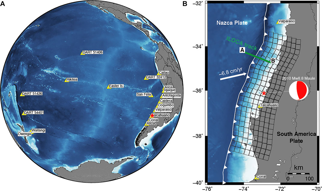
FIGURE 1. (A) Tsunami sensors (yellow triangles); (B) fault geometry (black squares), epicenter (red star) and average faulting geometry (red and white focal mechanism) of the 2010 Maule earthquake. A–B segment is the ILOCA track (green line).
These studies all find along-strike bilateral rupture from the epicenter, but vary significantly in the along-dip placement of slip on the fault, with most models that emphasize geodetic data having little slip far-offshore. It is well known that geodetic data can provide a good spatial resolution of fault slip very close to the stations, and along-strike for situations with good coastal-parallel coverage (e.g., Romano et al., 2010); but in subduction zones the resolution of offshore slip from land geodesy is typically very limited. Seismic wave models sometimes resolve offshore slip (e.g., Lay, 2018), but lacking seafloor geodetic observations, coseismic slip in the shallow region of the megathrust is usually best-constrained by tsunami data (e.g., Lorito et al., 2016) provided that accurate bathymetric models are available.
Tsunami data have long provided valuable constraints on the spatial extent of earthquake slip distributions due to them having the slowest propagation velocities of the various wave types (including seismic body and surface waves) used to study submarine sources. To exploit the absolute time information in deep-water and tide-gauge tsunami recordings for source inversions, one must trust the complete calculation of all known propagation effects through the heterogeneous bathymetric structure from the source region to the tsunami recording system. Absolute time alignments will then play a very strong role in the placement of slip in a finite-fault inversion. Errors in absolute travel time calculation due to both computational approximations (assumption of great-circle propagation for perturbation type corrections, use of inadequate bathymetry, etc.) and any clock errors in the recordings, will incorrectly align Green’s functions and data, biasing the inversion results.
Deep-water seafloor pressure sensors deployed at NOAA DART buoy sites often record clear tsunami waveforms that can be well-modelled by numerous finite-difference approaches, but absolute time misalignment has long been known to increase with source to station distance for commonly-used tsunami modeling codes, with modeled waveforms usually being earlier than observed signals. This is largely attributed to neglect of dispersion in the water column, neglect of elasticity of the rock substrate, neglect of water density profile, and, to a lesser extent, limitations of open ocean bathymetry models for the computed synthetics (Tsai et al., 2013; Watada et al., 2014). If uncorrected, use of absolute tsunami arrival times results in the placement of slip further from the observing stations to delay the tsunami arrivals, thus, erroneously shifting the source of slip landward. Recently, procedures have been introduced to account for some of these inadequacies of the computed tsunami signals (e.g., Tsai et al., 2013; Allgeyer and Cummins, 2014; Watada et al., 2014), which reduce the time alignment errors substantially, allowing use of absolute time information for deep-water buoy recordings in finite-fault inversions (Yue et al., 2014; Yoshimoto et al., 2016).
Time alignment shifts for tide-gauges are instead primarily attributed to clock errors or the use of inaccurate/coarse bathymetry models, mainly during the last portion of the propagation in very shallow water, and there is no set of correction procedures for the predictions to improve absolute time alignment of the tide-gauge observations. Often for tide-gauge data, the first-arrival times are picked in the data and held fixed, foregoing absolute time alignment, because the theoretical Green’s functions are so far off in timing. For linearized inversions, the a priori alignments of both deep-water (absolute times) and tide-gauge (fixed picks of arrivals), can have very strong influence on the solution.
Misalignment of predicted tsunami waveforms is a long-standing issue (e.g., Fujii and Satake, 2006; Piatanesi and Lorito, 2007), and for source inversions has typically been dealt with by manually aligning observed and predicted waveforms. However, this is a very subjective approach that directly negates the sensitivity of the tsunami timing to the placement of slip. The physics-based corrections used by Yue et al. (2014) and Yoshimoto et al. (2016), which allow absolute time alignments to be used in the inversions for deep-water sensors, are still imperfect, so some timing uncertainty can still be projected into the source model. This will be the case if the bathymetric model is inaccurate or too coarse. This is a very common situation for tide-gauges, which are generally installed within harbors or closed basins. The (generally) earlier arrival time of a modeled tide-gauge waveform on a coarse bathymetry depends mainly on two factors: 1) the tide-gauge position effectively being more offshore on a coarse computational grid with respect to a finer one and 2) the depth of the grid cell being deeper in coarser bathymetric models (e.g., Satake, 1995). Station clock errors can be another source of misalignment. The timing uncertainty can lead to inconsistent source images from deep-water vs. tide-gauge tsunami data or undesired averaging of results if both data types are used (e.g., Yoshimoto et al., 2016).
Given the limited precision of regional bathymetric models, tide-gauge data are often not used or are severely down-weighted in source inversions. These recordings, being widely distributed along the global coastline, can significantly contribute to enhancing the instrumental coverage around the tsunami source, thus prospectively helping to study tsunamigenic earthquakes. This is particularly important in those regions (e.g., the Mediterranean) where deep-water ocean sensors are not present, and only coastal gauges exist.
Romano et al. (2016) proposed a new method that can automatically deal with the waveform alignment issue through a procedure embedded into the inversion algorithm called Optimal Time Alignment (OTA). The method is partially borrowed from seismology, where time shift of seismic signals can result for different reasons (e.g., inaccuracies of the Earth seismic velocity model) and it can be estimated using the cross-correlation between observed and modeled signals (e.g., Zhang and Thurber, 2003; Hauksson and Shearer, 2005). The OTA method has two strengths: 1) it eliminates the arbitrariness in the time mismatch estimation, and 2) it is independent of the cause of the misalignment. OTA does not explicitly apply corrective terms to the tsunami propagation and can be used for both deep-water (e.g., DARTs) and coastal tide-gauge data.
The OTA method, already used for a few inversions (e.g., the 2016 Mw 8.3 Illapel and the 1960 Mw 9.5 Chile earthquakes, Romano et al., 2016; Ho et al., 2019), foregoes absolute time alignments and subjective fixed picks of arrival times of tide gauge data, recognizing that there is loss of absolute timing sensitivity, but reducing the strongly biasing effect of inaccurate time prediction. This approach requires an iterative non-linear search of the solution space; a linearized inversion is not viable. The optimal time alignments are re-determined in each iteration; they are not held fixed at initial subjective values. For the optimization performed by Romano et al. (2016), waveform variations for both deep-water and tide gauge stations originating from the different placement of slip on the kinematic model provide information that allows a self-consistent model to be found without the strong influence and bias of inaccurate absolute time alignment or fixed onset specification.
In this study, with the aim of benchmarking the OTA method against documented shallow seafloor deformation for the 2010 Maule earthquake, we repeat the study of Lorito et al. (2011) leaving everything unchanged except for the application of OTA to the tsunami signals. In this way we address the effect of OTA on the absolute placement of the slip patches relative to the prior study. We estimate the slip distribution of the 2010 Maule earthquake jointly inverting geodetic (GPS, InSAR, and land-leveling) and tsunami (DART and tide-gauge) data. In particular, the slip models and the predicted seafloor deformation obtained with and without the use of OTA are compared with the Yue et al. (2014) joint inversion model and the seafloor deformation data collected by Maksymowicz et al. (2017). We also investigate the effect of OTA in the joint inversion using DART and tide-gauge tsunami waveforms separately to assess their respective resolving power on the slip distribution, and, as a consequence, optimize their relative weights for use during joint inversion. Finally, we better constrain the slip distribution of the 2010 Maule earthquake by supplementing the initially inverted data set with additional GPS data from Vigny et al. (2011) and Moreno et al. (2012).
Material and Methods
Data and Green’s Functions
The subduction interface in the Maule region extends along the plate boundary from ∼39°S to ∼33°S and is parameterized (Figure 1; Figure S3, Table S1 in Supplementary Material) with a tessellation of 200 subfaults of 25 × 25 km2 size featuring variable strike and dip values that roughly follow the best-fitting non-planar geometry built from the global CMT mechanisms in the region (https://earthquake.usgs.gov/earthquakes/eventpage/official20100227063411530_30/technical).
We use the tsunami recordings (Supplementary Table S5) from 15 tide-gauges (provided by the Intergovernmental Oceanographic Commission of UNESCO, http://www.ioc-sealevelmonitoring.org/, the University of Hawaii sea level center (http://ilikai.soest.hawaii.edu/uhslc/background.html), and 4 DART buoys (National Oceanic and Atmospheric Administration, http://www.ndbc.noaa.gov/dart.shtml), and the coseismic deformation observed from GPS stations, satellites, and land-leveling. In particular, we use the coseismic offsets measured at 6 GPS sites managed by the International Global Navigation Satellite Systems Service (http://igscb.jpl.nasa.gov/) and the French Centre National de la Recherche Scientifique Institut National des Sciences de l'Univers (https://gpscope.dt.insu.cnrs.fr/), the GPS coseismic offsets provided by (Vigny et al., 2011; Moreno et al., 2012), the deformation along both the ascending and descending Line-of-Sight tracks obtained from the ALOS PALSAR satellite interferograms (http://global.jaxa.jp/), and the land-level changes measured along the Chilean coast from Farías et al. (2010). Additional details about the data processing can be found in Lorito et al. (2011), whereas input data are available as Supplementary Material (see Data Availability Statement).
Tsunami Green’s functions are computed with the nonlinear shallow water version of COMCOT (Liu et al., 1998), using a bathymetric grid model (http://topex.ucsd.edu/WWW_html/srtm30_plus.html) with 2 arc-min spatial resolution for deep-water tsunami propagation, and a system of nested grids with 30 arc-sec spatial resolution around each tide-gauge. The tsunami initial condition for each subfault (i.e., the vertical seafloor deformation) as well as the geodetic Green’s functions are computed using the dislocations in a half-space model (Okada, 1992).
Inversion
We estimate the coseismic slip distribution (slip and rake angle) by performing a nonlinear joint inversion of tsunami, GPS, InSAR and land-level data by using the Heat-Bath algorithm, a particular implementation of the Simulated Annealing technique, as global optimization method (Sen and Stoffa, 2013; more details in Supplementary Material). We assume a circular rupture front with constant expansion velocity VR = 2.25 km/s (Lay et al., 2010), consequently we shift the tsunami Green’s functions accordingly. The same VR value was adopted by Lorito et al. (2011), where preliminary tests had indicated that the current data configuration cannot constrain the rupture velocity for this event.
A different misfit function is used for each dataset. For geodetic data, an L2-norm is used. For tsunami data, we use a nonlinear cost-function sensitive to both waveform amplitude and period (Piatanesi and Lorito, 2007) modified for the OTA method by the introduction of the time parameter T (Romano et al., 2016):
In the cost function (1) obs and synt represent the observed and predicted tsunami signals, respectively, in a time window delimited by t1 and t2; the time parameter T introduces uniform time-shifts between each observed and predicted tsunami waveform during the inversion. Positive T values correspond to an earlier arrival of the synthetics. Here we assume that the main error sources are the locally coarse bathymetry around the tide-gauges and the modeling approximations for the DARTs. The clock errors are considered negligible, but if any exist they will map into the values of T.
The inverse problem is regularized by adding smoothing (through a Laplacian operator) and seismic moment minimization (using the total slip as a proxy for the seismic moment) constraints.
Lastly, the nonlinear approach allows us to present an average slip model instead of the best one, which could be an outlier not representative of the suite of solutions; this also provides a way to deal with inversion uncertainty (further details are discussed in Piatanesi and Lorito, 2007). The average model is obtained as a weighted mean of a subset of models (ensemble) that satisfactorily fit the data; in particular, the average slip distribution is computed by weighting the models within the ensemble by the inverse of their cost function values.
Results
The Effect of OTA When Inverting DARTs and/or Tide-gauge Data–A Synthetic Case
Extensive use of recordings from deep-water buoy recordings (DART) in inversions has significantly contributed to the understanding of large tsunami sources in the last decade. Being located in the open ocean, DART signals are simpler to model and contain clear waveform information about the source compared to tide-gauge observations, which are complicated by coastal and harbor effects. However, tide-gauges are more abundant than DARTs, so they are desirable for source studies. Strategies to increase their use and to overcome the modeling limitations, due, for example, to coarse bathymetry models and high computational cost of high-resolution simulations, are needed.
To address the relative importance of these two tsunami data sets for the specific case of the Maule earthquake, and to analyze the performance of OTA for different causes of misalignment, we perform a resolution test. We attempt to recover a target slip distribution featuring a checkerboard pattern (0 and 10 m slip alternating on groups of 3 × 3 subfaults, Figure 2A) by jointly inverting geodetic and either 1) all DART or 2) all tide-gauge, or 3) all DART and tide-gauge data. The checkerboard slip model is used to generate synthetic tsunami and geodetic (InSAR, GPS, land-leveling) signals that we use as “observations” in the inversions. Each dataset is corrupted by adding Gaussian random noise with a variance of 10% of the clean data. We also shift in time the target synthetic tsunami waveforms by adding a random delay in a range of 0–15 min to mimic the typically observed early arrival of the predicted tsunami signals. An additional sensitivity test is performed using an alternative set of tsunami Green’s functions computed with a bathymetric model around the tide-gauges with a lower spatial resolution (2 arc-min). This is tested against a checkerboard target model where the tsunami waveforms at the tide-gauges are produced using a bathymetry with a 0.5 arc-min spatial resolution; in this way, we do not add random delay to the tide-gauges because it is assumed to be intrinsic in the change of bathymetry, whereas we assume physics-like delays to the DARTs. In all of the cases, we perform the inversion with and without OTA.
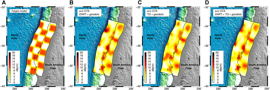
FIGURE 2. Target slip model (A); slip models estimated by jointly inverting geodetic and DART data (B), geodetic and tide-gauge data (C), geodetic, DART, and tide-gauge data (D). All of the inversions have been performed without using OTA.
Synthetic Test-Joint Inversions (Geodetic + DARTs and/or Tide-gauge Data) Without Using OTA
When the inversion is performed in a standard way, that is without OTA, the target slip model is never satisfactorily recovered on the entire fault (Figure 2). The inverted slip model is similar to the target only in the down-dip inland portion of the fault, which is where geodetic data, as expected, have a higher resolving power (Romano et al., 2020). To quantify the comparison between the estimated slip models and the target we calculate the Structural Similarity Index (SSIM; Giraud et al., 2018); we observe that all of the models have an index far from 1 (i.e., perfect match), specifically SSIMDART_woOTA = 0.20, SSIMTG_woOTA = 0.39, and SSIMJOINT_woOTA = 0.25. These discrepancies are confirmed by comparisons between the synthetic “observed” and predicted data that clearly present a time mismatch between the tsunami waveforms (Figures S4–S6 in Supplementary Material).
Synthetic Test-Joint Inversions (Geodetic + DARTs And/or Tide-gauge Data) Using OTA
When we apply OTA the target model is very well reconstructed independently of the data set combination used (Figure 3). Indeed, all SSIM values are significantly larger with respect to the previous cases (SSIMDART_wOTA = 0.67, SSIMTG_wOTA = 0.63, and SSIMJOINT_wOTA = 0.70). The results of these tests (as further documented by the very good agreement in the data comparisons in Supplementary Material Figures S7–S9) indicate that the joint inversion of all data sets with OTA used for the tsunami observations is the case that best reproduces the target model. We also observe that the slip distributions for inversions using only the DARTs or only the tide-gauges are similar to the joint inversion with both data sets, as indicated by the SSIM values. This indicates that OTA is equally effective for both DART and tide-gauge data, even though the reasons for the time misalignment are different. This surprisingly suggests that, in principle, there is no reason to prefer one tsunami data set over another in the inversion in this specific case and for this parameterization. However, uncertainties potentially affecting forward modeling are not fully taken into account by this type of synthetic test, since the “observed” and predicted tsunamis are modeled with the same Green’s functions, in contrast to an inversion using actual tsunami observations. These uncertainties are likely smaller for open-ocean tsunami numerical modeling at DART buoys. To address this issue, we perform an additional test.
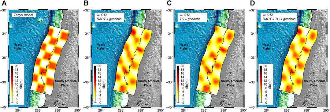
FIGURE 3. Target slip model (A); slip models estimated by jointly inverting geodetic and DART data (B), geodetic and tide-gauge data (C), geodetic, DART, and tide-gauge data (D). All of the inversions have been performed using OTA.
Synthetic Test-Joint Inversions (Geodetic + DARTs and Tide-gauge Data) With and Without Using OTA, Considering Tsunami Green’s Functions Computed on a Lower Resolution Bathymetry
In this test the tsunami Green’s functions for all of the stations (DARTs and tide-gauges) are computed by simulating the wave propagation on a bathymetric grid with 2 arc-min spatial resolution, whereas the “observed” tsunami waveforms are computed using a 30 arc-sec bathymetry around the tide-gauges; this is a sensitivity test to check how well the OTA works using Green’s functions recorded at a coarser spatial resolution with respect to the “real observations”. Differently from the tests shown in the previous sections, here the target tsunami waveforms at the tide-gauges are not corrupted with a random delay because this is implicit in the different bathymetry used with respect to the one adopted for the Green’s functions; on the other hand, since the possible delay to the DARTs is not related to the change of bathymetry then we add to these waveforms a “physics-like” delay that increases with the source-station distance.
The results of the tests show that without using OTA the target slip distribution is well reproduced for the portion of the fault closest to the geodetic observational points, which is consistent with the previous tests (compare Supplementary Material Figure S10B with Figure 2), whereas the resolution degrades with distance from the coastline; the comparison between observed and predicted data confirms this result (Supplementary Material Figure S11). When we apply the OTA then the checkerboard pattern is well recovered (Supplementary Material Figure S10C) and also the data fit improves (Supplementary Material Figure S12). It is important to notice how the change of bathymetry in some case affects the waveshape of the tide-gauges, but this appears to have a second-order effect on the target slip distribution that is nonetheless well reproduced.
The effect of OTA when inverting DARTs and/or tide-gauge data–The 2010 Mw8.8 Maule earthquake
Having verified, through the foregoing synthetic resolution test, the effectiveness of OTA in estimating the earthquake source when tsunami waveforms are affected by unmodelled time shifts alone, we now assess the performance of the method for the 2010 Mw8.8 Maule earthquake. We follow the same workflow adopted for the synthetic test.
Maule Earthquake-Joint Inversions (Geodetic + DARTs And/or Tide-gauge Data) Without Using OTA
Without using OTA, the inferred slip patterns for the three dataset combinations feature along-strike bilateral ruptures with 2 main patches of slip (Figure 4). The main asperity is located to the north of the epicenter and has a spatial extent of ∼250 km with a maximum slip value of ∼19 m at ∼35°S; a second and smaller asperity is located south of the epicenter and features as maximum slip ∼10 m in the area of the Arauco Peninsula, ∼37°S. The average rake is ∼111°, consistent with the slightly oblique relative convergence direction of the Nazca and South America plates. Visual comparison of the models in Figure 4 highlights the first-order similarity of the slip patterns. The DART and tide-gauge data would appear to have comparable resolving power for this earthquake, as was found for the synthetic tests; however, the SSIM values indicate that the slip model from joint inversion of geodetic and DART data (Figure 4A, SSIMDART_woOTA = 0.94) is more similar to the model using geodetic and all tsunami data (Figure 4C; Supplementary Table S3) than to that using geodetic and tide-gauge data together (Figure 4B, SSIMTG_woOTA = 0.74). In all cases, comparisons between observed and predicted data highlight good agreement for the geodetic data sets, but significant time-mismatches in the tsunami waveforms (Supplementary Material Figures S13–S15).
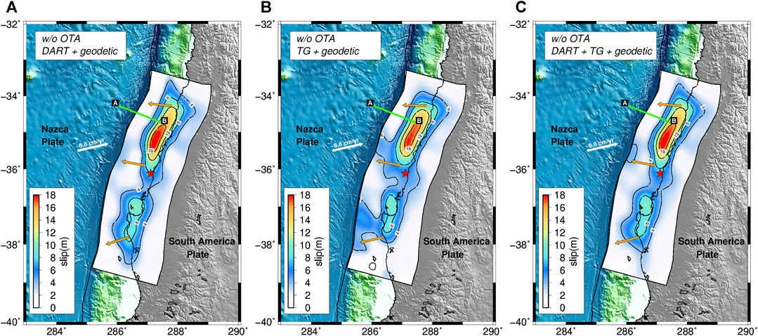
FIGURE 4. Rupture models of the 2010 Maule earthquake. Slip models (4 m contour lines in black) are estimated by jointly inverting geodetic and DART data (A), geodetic and tide-gauge data (B), geodetic, DART, and tide-gauge data (C). Red star represents the epicenter of the Maule earthquake; orange arrows represent the average slip directions (rake); green line represents the ILOCA track. All of the inversions have been performed without using OTA.
Maule Earthquake-Joint Inversion With a Priori Time-Shifts Corrections for Tide-gauges
Because of the time-mismatch present in the tsunami waveforms, we decide to follow the approach presented in Lorito et al. (2011), where they jointly inverted geodetic and tsunami data after correcting the Green’s functions for tide-gauges by applying a rigid time-shift to the signals. Lorito et al. (2011) conducted their work before studies on the travel time anomalies in the open ocean for distant tsunamis (Tsai et al., 2013; Watada et al., 2014). Hence, the underlying assumption of that approach was that the tsunami modeling of the tide-gauges signals, as described in the Introduction section, can be inaccurate due to several factors (e.g., the low-resolution bathymetry model around the instrument), whereas the DART signals modeling, being in principle more simple and accurate, does not necessitate any correction.
Notwithstanding the time-mismatch corrections for the tide-gauges, the slip distribution estimated following this approach (Figure 5A) has a rupture pattern very similar to the above slip models obtained without using OTA (Figure 4). Thus, the data fit continues to be very good for the geodetic data sets, whereas, apart from some tide-gauges that benefit from ad hoc time correction, the comparisons between observed and predicted tsunami waveforms still highlight a mismatch between the signals (Supplementary Material Figure S16).
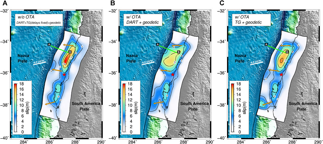
FIGURE 5. Rupture model of the 2010 Maule earthquake. Slip model (4 m contour lines in black) estimated by repeating the study of Lorito et al. (2011), jointly inverting geodetic, DART, and tide-gauge data without OTA but applying ad hoc rigid time shifts to the tide-gauges waveforms (A). Slip models estimated by joint inversion of geodetic and DART data (B), and joint inversion of geodetic and tide-gauge data (C). Red star represents the epicenter of the Maule earthquake; orange arrows represent the average slip directions (rake); green line represents the ILOCA track. The inversions in (B) and (C) have been performed using OTA.
Maule Earthquake-Joint Inversions (Geodetic + DARTs and/or Tide-gauge Data) Using OTA
Because of the persistent time-mismatch in the tsunami signals, we incorporate OTA in the joint inversions using the geodetic data and either the DARTs or the tide-gauges. The estimated slip distributions (Figures 5B,C) are significantly different from the models retrieved without OTA; the rupture area is still bilaterally distributed along strike, but the northern patch now shows relatively lower and more spatially spread slip (maximum values of ∼14 m and ∼16 m using DARTs or tide-gauges respectively, Figures 5B,C). In particular, both models are characterized by shallower rupture extent, with the model using DARTs having slip that reaches the trench for both the northern and southern patches.
Despite the comparable resolving power exhibited applying the OTA for the synthetic tests, significant differences are evident between slip distributions obtained using the DARTs or the tide-gauges. We also note that the tsunami time-mismatch corrections for the OTA inversion using DARTs (Supplementary Material Figure S17) are larger than those for the OTA inversion using tide-gauges (Supplementary Material Figure S18). This is consistent with the fact that the slip distribution in Figure 5C is closer to the coast compared to that in Figure 5B.
Finally, when we invert the complete set of data using OTA, the resulting slip distribution (Figure 6; Supplementary Table S2) confirms a bilateral rupture propagation with coseismic slip that extends to the shallow part of the subduction interface near the trench with slip greater than 8 m (maximum slip value ∼14 m); the second patch, around the Arauco Peninsula, features a maximum slip of ∼10 m, and the average rake angle is ∼113°, again consistent with the average relative plate convergence direction.
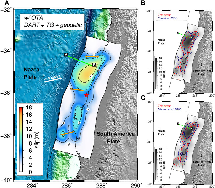
FIGURE 6. (A) Rupture model of the 2010 Maule earthquake estimated by jointly inverting geodetic, DART, tide-gauge data, and applying OTA. Solid black lines shows the slip contour at 4 m interval; red star represents the epicenter of the Maule earthquake; orange arrows represent the average slip directions (rake); green line represents the ILOCA track. The figure also shows the comparison between the 5m slip contour lines from the model (red line) presented in panel (A) and the model (blue line) by (B)Yue et al. (2014) and (C)Moreno et al., (2012).
Assuming a rigidity μ = 30 GPa the seismic moment is M0 = 1.73 × 10²² Nm (Mw = 8.8). Approximately the same value of moment magnitude Mw is found for all Maule earthquake slip models retrieved in the present study, with and without OTA.
The comparison between the observed and predicted data (Figures 7–9) is good for all of the data sets. In particular, the comparisons of tsunami waveforms (Figure 7) highlight an average time-shift of ∼5 min for the tide-gauges, compatible with uncertainties in the local bathymetry and tide-gauge locations (Romano et al., 2016); we also note that there is not an obvious station distance-delay relation (Figure 10) which supports the notion that for tide-gauges the shifts are dominated by local modeling inaccuracy near the stations. In contrast, the time mismatches found for the DART buoys increase with source-station distance (Figure 1A) and are on average ∼1% of the first arrival time (Figure 10), as observed by Watada et al. (2014). This is consistent with unmodeled features of the tsunami propagation (dispersion, ocean floor elasticity, water density variation with depth) for which Yue et al. (2014) applied theoretical corrections assuming tsunami propagation along great circles.
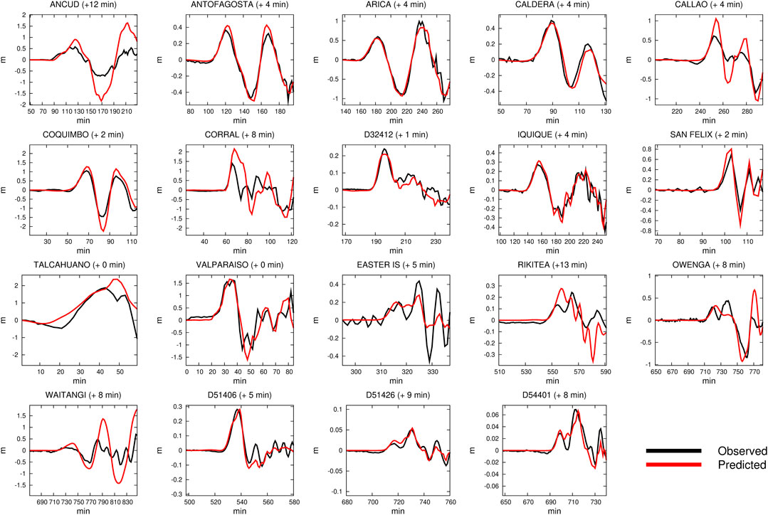
FIGURE 7. Comparison between observed (in black) and predicted (in red) tsunami waveforms for the slip distribution obtained by jointly inverting geodetic and tsunami data using OTA (Figure 6); the time mismatch estimated by the OTA is indicated within brackets.
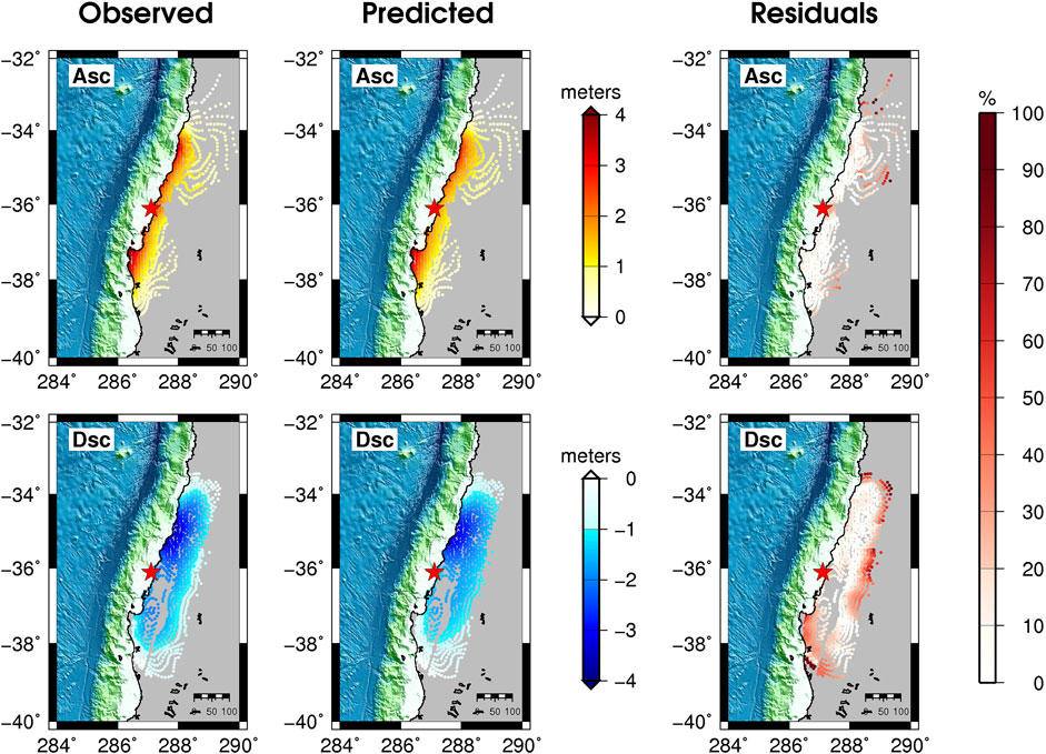
FIGURE 8. Comparison between observed, predicted, and percentage residuals of ascending (upper panels) and descending (bottom panels) InSAR data for the slip distribution obtained by jointly inverting geodetic and tsunami data using OTA (Figure 6).
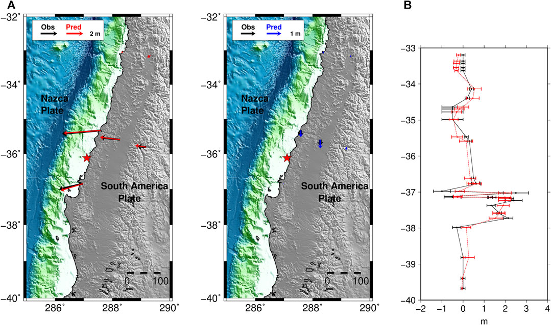
FIGURE 9. GPS and land-level data fit for the slip model shown in Figure 6. Comparison between observed (in black) and predicted (A) GPS data (horizontal and vertical in red and blue, respectively); (B) observed (black) and predicted (red) land-level changes; error bars for observations are experimental uncertainties, whereas for predictions they are calculated adding ±1σ errors.
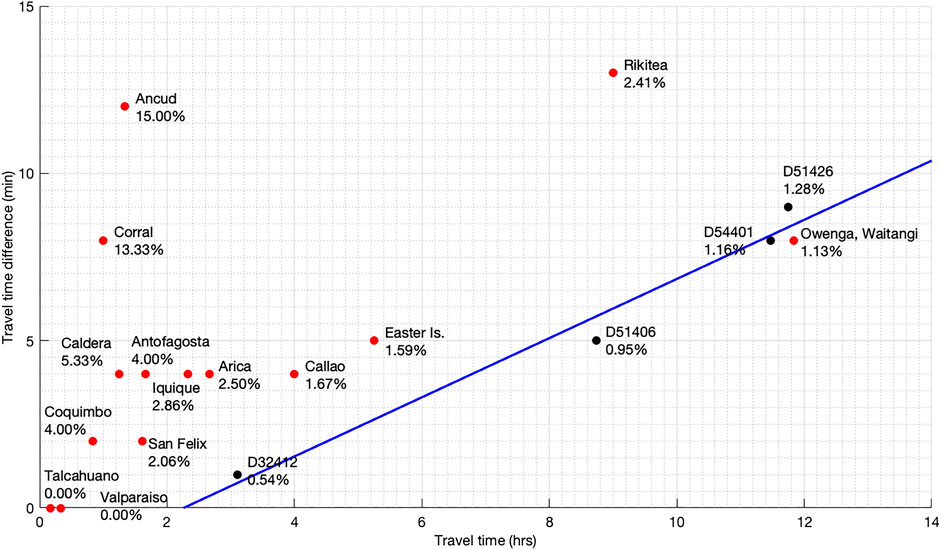
FIGURE 10. Time-shift (absolute and percentage) estimated for DART buoys (black dots) and tide-gauges (red dots) using the OTA method in the inversion shown in Figure 6 plotted vs. the observed arrival time. The blue line shows a systematic trend with distance for the DART data.
A comparison with the slip models by Moreno et al. (2012) and Yue et al. (2014) shows that the along-strike extent of the rupture area estimated using the OTA is comparable with both the models, as well as the northern location of the main asperity; however, while reaching the trench, the shallow slip of our model is slightly lower (∼10 m) than the (Yue et al. (2014), >15 m) model (Figures 6B,C). The difference in the maximum slip value might be ascribed to the fact that the model by Yue et al. (2014) is obtained without inverting tide-gauge data; indeed, the maximum shallow slip value (Figure 5B) estimated inverting geodetic and DART waveforms only [i.e., a data configuration similar to Yue et al. (2014)] is higher (∼12 m) and closer to the Yue et al. (2014) value.
As anticipated in Data and Green’s functions, to account for non-uniqueness of the solution, for each inversion we show the average slip model (obtained as a weighted mean of a subset of models featuring the lowest cost functions) instead of the best model (the one with the lowest cost function) that could represent an “extreme” best fitting case. To emphasize potentially equivalent parameter values, the analysis of the model ensemble is illustrated in the form of marginal distributions of the slip for each subfault (Supplementary Material Figure S19), featuring a Gaussian shape centered on the average slip value, highlighting how the slip is well resolved over the entire fault plane. This is true also for the slip distributions obtained from the joint inversion of geodetic and tsunami data without using OTA. However, comparing the marginal distributions of the two slip models (i.e., with and without OTA) we argue that the shallow slip found using OTA is not an artifact (or an outlier) of the inversion; it rather is evident that the average slip values in the northern and larger asperity show systematic behavior moving toward the shallow part of the fault. This can be observed from another point of view through the evolution of the models explored by the algorithm during the inversion (see Movies S1, S2 in Supplementary Material) displaying how the inversion, as the cost function decreases, converges toward a solution that features shallow slip in the model using OTA, and the slip is forced to locate deeper in the other case.
On the other hand, significant differences are evident down-dip in the southern patch of slip; specifically, the southern asperity estimated in the model proposed here, as well as the one by Moreno et al. (2012) does not reach the shallow part of the subduction interface, whereas the slip model proposed by Yue et al. (2014) highlights a coseismic dislocation of ∼10 m close to the trench around 37°S. To address if these differences may be ascribable to the different GPS data set used by Yue et al. (2014) we perform an additional inversion incorporating these data.
Maule Earthquake-Joint Inversion (Geodetic + DARTs and Tide-gauge Data) Using OTA and a Larger GPS Data Set
Using the OTA, we jointly invert the previous data sets supplementing them with the GPS coseismic offsets used by Moreno et al., (2012) and Yue et al., (2014), whose spatial distribution is denser and might help to better constrain the slip distribution.
The resulting slip distribution (Figure 11; Supplementary Table S4) confirms both the along-strike extent of the rupture area and the bilateral rupture propagation with respect to the hypocenter. Whereas the northern asperity continues to be characterized by large slip extending to the shallow part of the subduction interface with second-order differences with respect to the model proposed in Figure 6, the asperity located to the south of the hypocenter is not confined close to the Arauco Peninsula, but features significant slip (∼8–10 m) up to the trench. Thus, this updated slip model of the Maule earthquake is similar to the model proposed by Yue et al., (2014) (Figure 11B); this is consistent with the fact that, in this case, the data sets used in both models are similar (Yue et al. (2014) included teleseismic data, but did not include tide gauge data). The comparison between the observed and predicted data is satisfactory for all of the data sets (Figures 12–14). The seismic moment corresponding to the slip model in Figure 11 is M0 = 1.76 × 10²² Nm (Mw = 8.8).
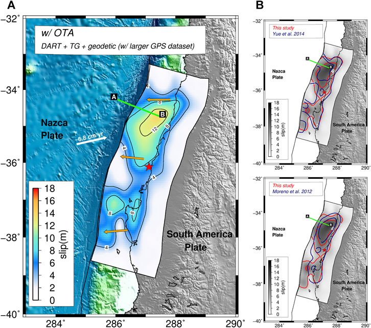
FIGURE 11. (A) Rupture model of the 2010 Maule earthquake estimated by jointly inverting geodetic, DART, tide-gauge data, and applying OTA; the GPS data set used in this case is larger than the one shown in Figure 9 and is the same used from (Moreno et al., 2012) and (Yue et al., 2014). Solid black lines shows the slip contour at 4 m interval; red star represents the epicenter of the Maule earthquake; orange arrows represent the average slip directions (rake); green line represents the ILOCA track. The figure also shows the comparison between the 5 m slip contour lines from the model (red line) presented in panel (A) and the model (blue line) by (B)Yue et al. (2014) and (C)Moreno et al. (2012).
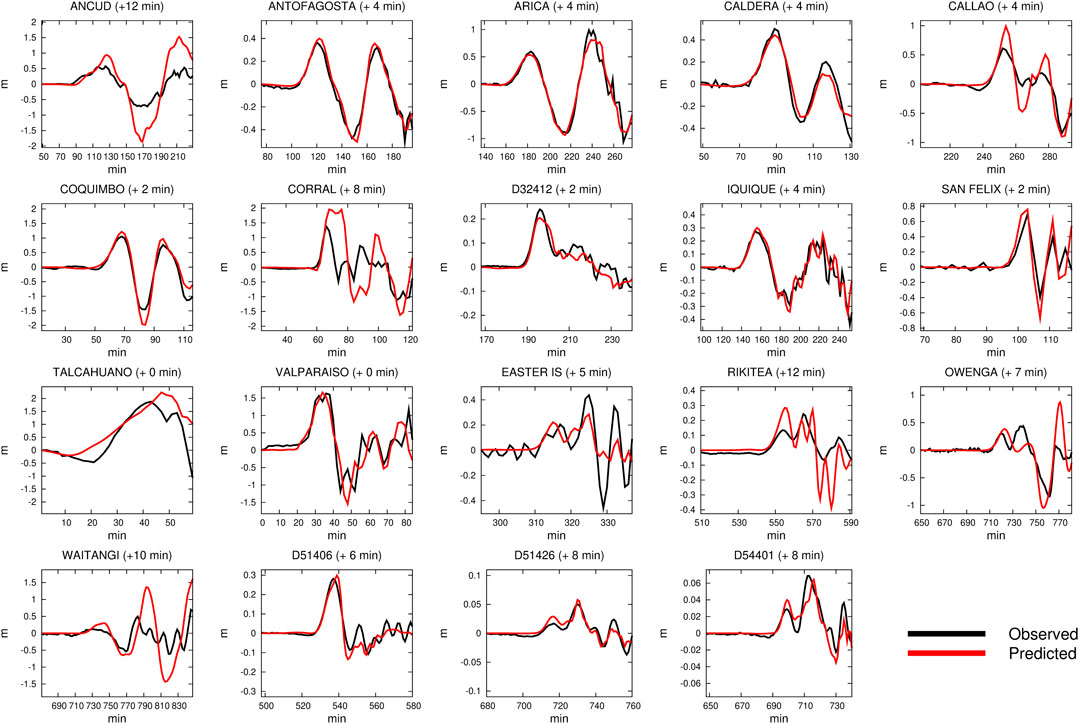
FIGURE 12. Comparison between observed (in black) and predicted (in red) tsunami waveforms for the slip distribution obtained by jointly inverting the same GPS data set used from Moreno et al. (2012) and Yue et al. (2014), InSAR, land-leveling, and tsunami data using OTA (Figure 11); the time mismatch estimated by the OTA is indicated within brackets.
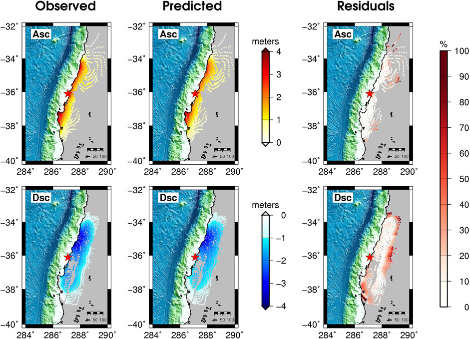
FIGURE 13. Comparison between observed, predicted, and percentage residuals of ascending (upper panels) and descending (bottom panels) InSAR data for the slip distribution shown in Figure 11.
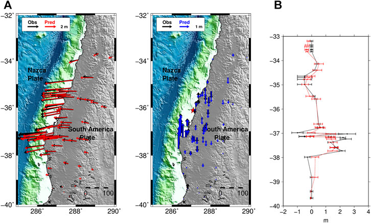
FIGURE 14. GPS and land-level data fit for the slip model shown in Figure 11. Comparison between observed (in black) and predicted (A) GPS data (horizontal and vertical in red and blue, respectively); (B) observed (black) and predicted (red) land-level changes; error bars for observations are experimental uncertainties, whereas for predictions they are calculated adding ±1σ errors.
Discussion
This study of the 2010 Maule earthquake shows that using OTA for the tsunami waveforms inversion can affect the final slip distribution. For the 2010 Maule earthquake some prior studies indicate significant slip in the shallow region of the megathrust (Yue et al., 2014) while others do not (Lorito et al., 2011). It is important to resolve the occurrence of large shallow earthquake slip either as part of a great rupture or as distinct shallow rupturing “tsunami earthquakes” (Kanamori, 1972), as this information is valuable for tsunami hazard analyses (Kozdon and Dunham, 2014; Murphy et al., 2016; Murphy et al., 2018; Grezio et al., 2017). The physics-based corrections Yue et al. (2014) applied to the modeled tsunami waveforms directly result in prediction of the existence of coseismic shallow slip nearby the trench. This has been confirmed by direct imaging of seafloor deformation (Maksymowicz et al., 2017). Hence, it became evident that a more accurate modeling strategy for the tsunami Green’s functions, which approximates the relevant physics (Tsai et al., 2013; Watada et al., 2014), should be used for slip inversions, at least in some specific cases.
Without using OTA, our slip distributions are similar to previously published coseismic rupture models that did not use any tsunami data (Delouis et al., 2010; Tong et al., 2010; Vigny et al., 2011; Moreno et al., 2012), and even more similar to those using tsunami data but without consideration of tsunami waveforms misalignments (Lorito et al., 2011). Conversely, with OTA, whereas the along-strike extent of the rupture area (Figure 6B,C) is still consistent with Yue et al. (2014) and Moreno et al. (2012), a significant amount of slip (∼10 m) shifts trenchward in the solution; this is similar to what was shown by Yue et al. (2014) after applying physics-based corrective terms to the deep-water tsunami Green’s functions (Figure 6B). This feature of the model is confirmed when the slip model is better constrained by a larger set of GPS data used in the inversion (Figure 11). The positive comparison with the slip model proposed by Yue et al. (2014) provides an encouraging confirmation that OTA works as an alternative to computing physics based corrections. More directly, the multi-beam bathymetric re-survey conducted by Maksymowicz et al. (2017) along a track named ILOCA (Figures 1, 4–6) measuring the vertical seafloor deformation produced by this megathrust earthquake offers an additional opportunity to benchmark the method.
Thus, we perform a forward prediction of both the vertical and horizontal components of the seafloor deformation associated with all the slip models investigated in the present study, comparing them against the observations (Figure 15). We also compare our results with the models by Tong et al. (2010) [hereinafter TO10], Yue et al. (2014) [YU14], and Yoshimoto et al. (2016) [YO16].
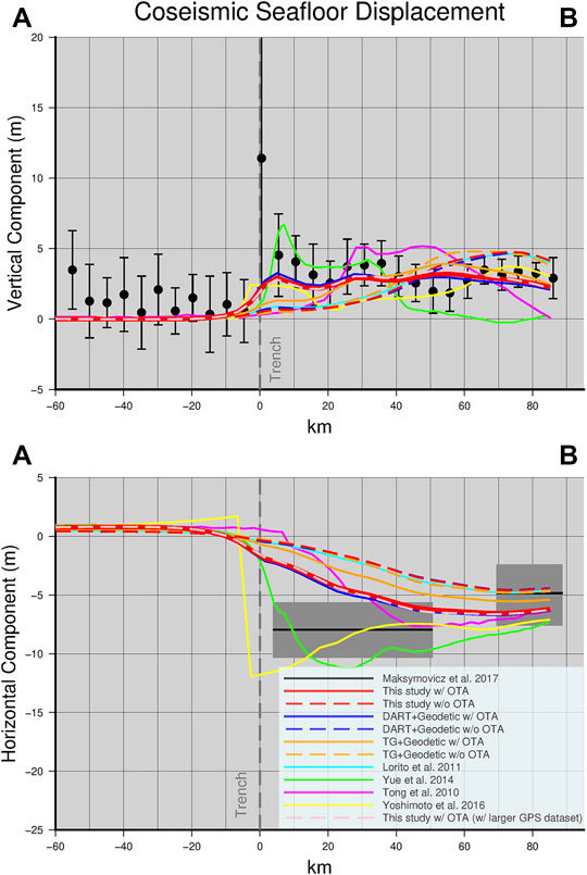
FIGURE 15. Comparison between observed (black) and predicted (A) vertical and (B) horizontal seafloor deformation along the ILOCA track; in (A) error bars indicate the standard deviation, whereas in (B) the approximated error bars are in grey. In both panels, predicted seafloor deformations are shown for the slip distributions obtained for all cases investigated in this study (with and without OTA along with predictions for the Yue et al. (2014, green), Tong et al. (2010, magenta), and Yoshimoto et al. (2016, yellow) models. Dashed grey vertical line in both the panels indicates the trench location along the ILOCA segment.
The comparisons in Figure 15 indicate that the slip models derived with OTA reproduce the data significantly better than the models without OTA. Large slip near the trench is needed to replicate the seafloor deformation along the ILOCA track. This is found for the slip distributions obtained by jointly inverting geodetic and all tsunami data, or geodetic and DARTs; indeed, these two models show similar predictions (Figures 5B, 6, 11) as expected given their similar slip distributions. On the other hand for the joint OTA inversion of geodetic and tide-gauge data, the comparison with deformation along the ILOCA track becomes satisfactory only along the segment more than ∼20 km from the trench. This is an indirect indication (or an a-posteriori verification) that the epistemic uncertainty of the DART data is less than for the tide-gauges. This is because the DART data require less-sophisticated (linear) modeling and inherently do not depend as critically on availability of high-resolution bathymetry models. This behavior motivates placing higher relative weight on the DART data in the inversion when using both data sets.
The comparison between the model with OTA and the YU14 model shows a pretty good agreement at least up to ∼40 km from the trench, whereas the YO16 model predicts a vertical deformation closer to the lower limit of the error bars. The difference in the maximum shallow slip in our and YU14 models might be responsible for the under- and over-estimation of the vertical deformation measured landward around 10 km from the trench, respectively; however, both the predictions are well within the error bars. We also note that none of the models reproduce the 10 + m vertical deformation at the trench; several reasons can explain this discrepancy. The rupture models may not fully capture slip right at the trench. Actually, these slip models have too coarse of resolution for capturing the narrow peak (e.g., YU14 model has a peak which is slightly displaced landward and it is also broader but smaller). Another explanation might be related to the near trench displacement not being captured by instantaneous and elastic deformation of homogeneous crust. Also the errors associated to the data, may be larger than estimated, or a combination of some of these factors. However, the more reasonable explanation appears to be related to the errors associated to the data being larger than estimated. Indeed, as discussed by Maksymowicz et al. (2017), the larger standard deviation of the data in peak slip zone prevents an exact interpretation of the deformation in that part of the ILOCA segment. A strong bathymetric gradient close to the trench can increase the noise of the swath bathymetry data and hence be the cause of the larger error in the estimated deformation. The discrepancy with the prediction by YU14 increases landward (i.e., toward point B in Figure 15), with our OTA prediction remaining within or very close to the error bars, whereas the YO16 model fits very well the deformation in the eastern ∼50 km of the segment. On the other hand, the deformation predicted by the models not using OTA do not match the vertical deformation in the trench region, similar to forward predictions for a model like TO10 based on only geodetic data. Otherwise, all models, with the possible exception of YU14, perform reasonably well landward along this profile. Measured horizontal seafloor deformation is characterized by larger uncertainty than vertical deformation (Maksymowicz et al., 2017). The comparison of the models with the horizontal deformation in Figure 15 nevertheless suggests a slightly higher consistency of OTA models with the direct deformation measurements than for the models obtained without using OTA.
The present study shows that for this earthquake and using this data set, the OTA method allows retrieval of a slip distribution consistent with both the model proposed by Yue et al. (2014), which applied physics based corrections to DART calculations and independently measured seafloor deformation. The OTA method can be applied if the Green’s functions are computed by either the most sophisticated methods that account for all known propagation effects (e.g., Ho et al., 2019) or by simplified procedures that give good waveshapes, but inaccurate travel times. There will always be errors in the model predictions (we cannot reproduce the Earth effects perfectly with any model), and there may be clock errors. OTA will adjust the time misalignments to avoid bias of the solution for the known and unknown limitations of the Green’s functions for the time alignment. As only time shifts are involved, inadequacies of the Green’s functions for predicting the waveshapes, particularly for tide-gauge recordings sensitive to detailed coastal bathymetry, are not accounted for by OTA. Only by improving the bathymetry models can those waveshape predictions be improved. But, the OTA method reduces the predicted arrival time errors for the first cycles of the tide gauge data, suppressing first-order bias in the inversions.
Of course, the epistemic uncertainty could still be reduced further with improved numerical modeling. Indeed, some modeling limitations might result from not using a more physically complete tsunami numerical model that, in general, would be preferable (Yamazaki et al., 2011; Allgeyer and Cummins, 2014) or more accurate modeling approaches for the tsunami generation (Kajiura, 1963; Nosov and Kolesov, 2011); however, our findings show that OTA approach works well given less complete computation of the tsunami Green’s functions. Additionally, the absolute slip estimates could be slightly affected by neglecting in the tsunami Green’s functions the contribution of the seafloor horizontal motion to the vertical uplift (Bletery et al., 2015) or by using elastically homogeneous materials instead of heterogeneous medium (Romano et al., 2014). The OTA method is used during the inversion to remove from the modeled tsunami signals any time-mismatch whose origin is unknown; once the tsunami waveforms are aligned with the observed signals then the inversion algorithm searches for the slip pattern that best fits amplitude and period of the tsunami waves. We emphasize that the OTA does not improve specific waveform shape mismatches such as the initial reverse polarity phase at distant DARTs (Watada et al., 2014) or arising from inadequate coastal bathymetry models which might change details of the slip distribution; however, these are commonly second order effects not projecting into the general rupture pattern.
Thus, when complete modeling of the tsunami wavefield (e.g. including high-resolution bathymetry, dispersion, the Earth’s elasticity, etc.) is not feasible or is computationally excessively demanding, the OTA method proves very effective for tsunami data (DARTs and/or tide-gauge) inversion. We observe that without using OTA a bias is introduced in the slip distribution that for the specific case of the Maule earthquake causes the slip to be artificially confined deeper. The resolution tests for the specific configuration of tsunami sensors demonstrate that DARTs and tide-gauges have comparable resolving power, despite the former being very limited in number; but the results of inversions for the Maule event indicate that DARTs have higher spatial sensitivity for mapping the coseismic slip. Thus, in principle, DART data are preferable to the tide-gauge data or at least deserve to be weighted more in the inversion. However, even if with a lower weight, the results here indicate that the tide-gauges data should not be excluded. If they are the only tsunami sensors available for studying a tsunamigenic event, they can be reliably inverted as long as one uses OTA to mitigate bias from incorrect time alignment (Ho et al., 2019). The experiments carried out, described, and discussed in the present study are summarized and represented also in the form of a flowchart in Supplementary Material Figure S20.
Conclusion
We reanalyze the 2010 Maule earthquake by jointly inverting geodetic (GPS, InSAR, land-level) and tsunami (DART, tide-gauge) data by incorporating the optimal time alignment (OTA) method in the inversion. This allows the estimation of the earthquake slip distribution taking into account, in an automatic and non-subjective way, the time mismatch between observed and predicted tsunami waveforms. The Maule earthquake offered an opportunity to benchmark the OTA method. The resulting rupture pattern confirms bilateral rupture propagation, including a significant amount of slip (∼10 m) near the trench within the northern slip patch, as previously indicated by (theoretical phase-corrected) DART data inversions. The presence of significant slip in the shallower portion of the subduction interface is supported by a comparison between seafloor deformation predicted for the OTA joint inversion estimated slip distribution and directly observed deformation for a repeated bathymetric survey off the Maule region. Finally, the inversion results show that DARTs outperform tide-gauges in estimating the slip distribution of a tsunamigenic event, giving an objective basis for the relative weights to be assigned in this type of joint inversion using the two data types.
Data Availability Statement
The original contributions presented in the study are included in the article/Supplementary Material, further inquiries can be directed to the corresponding author.
Author Contributions
FR was involved in all of the phases of this study. SL and TL contributed to design the Experiment, discuss and interpret the results, and to writing the manuscript. AP contributed to design the Experiment, discuss and interpret the results. MV, SM, and RT contributed to the tsunami data analysis and to discuss the results. All authors reviewed the final manuscript.
Funding
This work has been partially funded by EC project ASTARTE - Assessment, STrategy and Risk Reduction for Tsunamis in Europe. Grant 603839, 7th FP (ENV.2013.6.4-3 ENV.2013.6.4-3) and the Italian Flagship Project RITMARE. TL’s earthquake research is supported by U.S. National Science Foundation grant EAR1802364.
Conflict of Interest
The authors declare that the research was conducted in the absence of any commercial or financial relationships that could be construed as a potential conflict of interest.
Acknowledgments
We wish to thank the Intergovernmental Oceanographic Commission of UNESCO (IOC) (http://www.ioc-sealevelmonitoring.org/), the University of Hawaii sea level center (https://uhslc.soest.hawaii.edu), and the National Oceanic and Atmospheric Administration (NOAA, http://www.ndbc.noaa.gov/dart.shtml) for providing tsunami data; the Japan Aerospace Exploration Agency (http://global.jaxa.jp/) for providing the ALOS-PALSAR data; the International Global Navigation Satellite Systems Service and the French Centre National de la Recherche Scientifique - Institut National des Sciences de l’Univers (INSU, France, http://igscb.jpl.nasa.gov/) for providing GPS data (https://gpscope.dt.insu.cnrs.fr/). Figures in the main text and Supporting Information made use of GMT (https://www.generic-mapping-tools.org) and MATLAB (www.mathworks.com) software. We thank three anonymous reviewers for their valuable comments and suggestions.
Supplementary Material
The Supplementary Material for this article can be found online at: https://www.frontiersin.org/articles/10.3389/feart.2020.585429/full#supplementary-material.
References
Allgeyer, S., and Cummins, P. (2014). Numerical tsunami simulation including elastic loading and seawater density stratification. Geophys. Res. Lett. 41, 2368–2375. doi:10.1002/2014GL059348
Bletery, Q., Sladen, A., Delouis, B., and Mattéo, L. (2015). Quantification of tsunami bathymetry effect on finite Fault Slip inversion. Pure Appl. Geophys. 172, 3655–3670. doi:10.1007/s00024-015-1113-y
Delouis, B., Nocquet, J.-M., and Vallée, M. (2010). Slip distribution of the February 27, 2010 Mw = 8.8 Maule Earthquake, central Chile, from static and high-rate GPS, InSAR, and broadband teleseismic data. Geophys. Res. Lett. 37, 235. doi:10.1029/2010GL043899
Farías, M., Vargas, G., Tassara, A., Carretier, S., Baize, S., Melnick, D., et al. (2010). Land-level changes produced by the Mw 8.8 2010 Chilean earthquake. Science. 329, 916. doi:10.1126/science.1192094 |
Fritz, H. M., Petroff, C. M., Catalán, P. A., Cienfuegos, R., Winckler, P., Kalligeris, N., et al. (2011). Field survey of the 27 February 2010 Chile tsunami. Pure Appl. Geophys. 168, 1989–2010. doi:10.1007/s00024-011-0283-5
Fujii, Y., and Satake, K. (2013). Slip distribution and seismic moment of the 2010 and 1960 Chilean earthquakes inferred from tsunami waveforms and coastal geodetic data. Pure Appl. Geophys. 170, 1493–1509. doi:10.1007/s00024-012-0524-2
Fujii, Y., and Satake, K. (2006). Source of the July 2006 West Java tsunami estimated from tide gauge records. Geophys. Res. Lett. 33, 569. doi:10.1029/2006GL028049
Giraud, J., Pakyuz-Charrier, E., Ogarko, V., Jessell, M., Lindsay, M., and Martin, R. (2018). Impact of uncertain geology in constrained geophysical inversion. ASEG Extend. Abstr. 2018, 1–6. doi:10.1071/aseg2018abm1_2f
Grezio, A., Babeyko, A., Baptista, M. A., Behrens, J., Costa, A., Davies, G., et al. (2017). Probabilistic tsunami hazard analysis: multiple sources and global applications. Rev. Geophys. 55, 1158–1198. doi:10.1002/2017RG000579
Hauksson, E., and Shearer, P. (2005). Southern California hypocenter relocation with waveform cross-correlation, Part 1: results using the double-difference method. Bull. Seismol. Soc. Am. 95, 896–903. doi:10.1785/0120040167
Hayes, G. P., Bergman, E., Johnson, K. L., Benz, H. M., Brown, L., and Meltzer, A. S. (2013). Seismotectonic framework of the 2010 February 27 Mw 8.8 Maule, Chile earthquake sequence. Geophys. J. Int. 195, 1034–1051. doi:10.1093/gji/ggt238
Ho, T.-C., Satake, K., Watada, S., and Fujii, Y. (2019). Source estimate for the 1960 Chile earthquake from joint inversion of geodetic and transoceanic tsunami data. J. Geophys. Res. Solid Earth. 124, 2812–2828. doi:10.1029/2018JB016996
Kajiura, K. (1963). The leading wave of a tsunami. Bull. Earthq. Res. Inst. Univ. Tokyo. 41, 535–571.
Kanamori, H. (1972). Mechanism of tsunami earthquakes. Phys. Earth Planet. Int. 6, 346–359. doi:10.1016/0031-9201(72)90058-1
Koper, K. D., Hutko, A. R., Lay, T., and Sufri, O. (2012). Imaging short-period seismic radiation from the 27 February 2010 Chile (MW 8.8) earthquake by back-projection of P, PP, and PKIKP waves. J. Geophys. Res.: Solid Earth. 117, 289. doi:10.1029/2011JB008576
Kozdon, J. E., and Dunham, E. M. (2014). Constraining shallow slip and tsunami excitation in megathrust ruptures using seismic and ocean acoustic waves recorded on ocean-bottom sensor networks. Earth Planet Sci. Lett. 396, 56–65. doi:10.1016/j.epsl.2014.04.001
Lay, T. (2018). A review of the rupture characteristics of the 2011 Tohoku-oki Mw 9.1 earthquake. Tectonophysics. 733, 4–36. doi:10.1016/j.tecto.2017.09.022
Lay, T., Ammon, C. J., Kanamori, H., Koper, K. D., Sufri, O., and Hutko, A. R. (2010). Teleseismic inversion for rupture process of the 27 February 2010 Chile (Mw 8.8) earthquake. Geophys. Res. Lett. 37, 568. doi:10.1029/2010GL043379
Lin, Y. N., Sladen, A., Ortega‐Culaciati, F., Simons, M., Avouac, J.-P., Fielding, E. J., et al. (2013). Coseismic and postseismic slip associated with the 2010 Maule earthquake, Chile: characterizing the Arauco Peninsula barrier effect. J. Geophys. Res.: Solid Earth. 118, 3142–3159. doi:10.1002/jgrb.50207
Liu, P. L. F., Woo, S. B., and Cho, Y. S. (1998). Computer programs, for tsunami propagation and inundation, Technical report. Cornell University.
Lorito, S., Romano, F., Atzori, S., Tong, X., Avallone, A., McCloskey, J., et al. (2011). Limited overlap between the seismic gap and coseismic slip of the great 2010 Chile earthquake. Nat. Geosci. 4, 173–177. doi:10.1038/ngeo1073
Lorito, S., Romano, F., and Lay, T. (2016). “Tsunamigenic major and great earthquakes (2004–2013): source processes inverted from seismic, geodetic, and sea-level data,” in Encyclopedia of Complexity and systems science. Editor R. A. Meyers (Berlin, Heidelberg: Springer), 1–52. doi:10.1007/978-3-642-27737-5_641-1
Maksymowicz, A., Chadwell, C. D., Ruiz, J., Tréhu, A. M., Contreras-Reyes, E., Weinrebe, W., et al. (2017). Coseismic seafloor deformation in the trench region during the Mw8.8 Maule megathrust earthquake. Sci. Rep. 7, 45918. doi:10.1038/srep45918 |
Moreno, M., Melnick, D., Rosenau, M., Baez, J., Klotz, J., Oncken, O., et al. (2012). Toward understanding tectonic control on the Mw 8.8 2010 Maule Chile earthquake. Earth Planet Sci. Lett. 321 (322), 152–165. doi:10.1016/j.epsl.2012.01.006
Murphy, S., Di Toro, G., Romano, F., Scala, A., Lorito, S., Spagnuolo, E., et al. (2018). Tsunamigenic earthquake simulations using experimentally derived friction laws. Earth Planet Sci. Lett. 486, 155–165. doi:10.1016/j.epsl.2018.01.011
Murphy, S., Scala, A., Herrero, A., Lorito, S., Festa, G., Trasatti, E., et al. (2016). Shallow slip amplification and enhanced tsunami hazard unravelled by dynamic simulations of mega-thrust earthquakes. Sci. Rep. 6, 35007. doi:10.1038/srep35007 |
Nosov, M. A., and Kolesov, S. V. (2011). Optimal initial conditions for simulation of seismotectonic tsunamis. Pure Appl. Geophys. 168, 1223–1237. doi:10.1007/s00024-010-0226-6
Okada, Y. (1992). Internal deformation due to shear and tensile faults in a half-space. Bull. Seismol. Soc. Am. 82, 1018–1040.
Piatanesi, A., and Lorito, S. (2007). Rupture process of the 2004 sumatra–Andaman earthquake from tsunami waveform inversion. Bull. Seismol. Soc. Am. 97, S223–S231. doi:10.1785/0120050627
Pollitz, F. F., Brooks, B., Tong, X., Bevis, M. G., Foster, J. H., Bürgmann, R., et al. (2011). Coseismic slip distribution of the February 27, 2010 Mw 8.8 Maule, Chile earthquake. Geophys. Res. Lett. 38, 735. doi:10.1029/2011GL047065
Romano, F., Lorito, S., Piatanesi, A., and Lay, T. (2020). “Fifteen years of (major to great) tsunamigenic earthquakes” in Reference module in earth systems and environmental sciences. New York: Elsevier. doi:10.1016/B978-0-12-409548-9.11767-1
Romano, F., Piatanesi, A., Lorito, S., and Hirata, K. (2010). Slip distribution of the 2003 Tokachi-oki Mw 8.1 earthquake from joint inversion of tsunami waveforms and geodetic data. J. Geophys. Res. Solid Earth. 115, 648. doi:10.1029/2009JB006665
Romano, F., Piatanesi, A., Lorito, S., Tolomei, C., Atzori, S., and Murphy, S. (2016). Optimal time alignment of tide-gauge tsunami waveforms in nonlinear inversions: application to the 2015 Illapel (Chile) earthquake. Geophys. Res. Lett. 43 (11), 226–311. doi:10.1002/2016GL071310
Romano, F., Trasatti, E., Lorito, S., Piromallo, C., Piatanesi, A., Ito, Y., et al. (2014). Structural control on the Tohoku earthquake rupture process investigated by 3D FEM, tsunami and geodetic data. Sci. Rep. 4, 5631. doi:10.1038/srep05631 |
Satake, K. (1995). Linear and nonlinear computations of the 1992 Nicaragua earthquake tsunami. PAGEOPH. 144, 455–470. doi:10.1007/BF00874378
Sen, M. K., and Stoffa, P. L. (2013). Global optimization methods in geophysical inversion. Cambridge: Cambridge University Press. doi:10.1017/CBO9780511997570
Tong, X., Sandwell, D., Luttrell, K., Brooks, B., Bevis, M., Shimada, M., et al. (2010). The 2010 Maule, Chile earthquake: downdip rupture limit revealed by space geodesy. Geophys. Res. Lett. 37, 235. doi:10.1029/2010GL045805
Tsai, V. C., Ampuero, J.-P., Kanamori, H., and Stevenson, D. J. (2013). Estimating the effect of Earth elasticity and variable water density on tsunami speeds. Geophys. Res. Lett. 40, 492–496. doi:10.1002/grl.50147
Vigny, C., Socquet, A., Peyrat, S., Ruegg, J.-C., Métois, M., Madariaga, R., et al. (2011). The 2010 Mw 8.8 Maule megathrust earthquake of Central Chile, monitored by GPS. Science. 332, 1417–1421. doi:10.1126/science.1204132 |
Watada, S., Kusumoto, S., and Satake, K. (2014). Traveltime delay and initial phase reversal of distant tsunamis coupled with the self-gravitating elastic Earth. J. Geophys. Res. Solid Earth. 119, 4287–4310. doi:10.1002/2013JB010841
Yamazaki, Y., Cheung, K. F., and Kowalik, Z. (2011). Depth-integrated, non-hydrostatic model with grid nesting for tsunami generation, propagation, and run-up. Int. J. Numer. Methods Fluid. 67, 2081–2107. doi:10.1002/fld.2485
Yoshimoto, M., Watada, S., Fujii, Y., and Satake, K. (2016). Source estimate and tsunami forecast from far-field deep-ocean tsunami waveforms—the 27 February 2010 Mw 8.8 Maule earthquake. Geophys. Res. Lett. 43, 659–665. doi:10.1002/2015GL067181
Yue, H., Lay, T., Rivera, L., An, C., Vigny, C., Tong, X., et al. (2014). Localized fault slip to the trench in the 2010 Maule, Chile Mw = 8.8 earthquake from joint inversion of high-rate GPS, teleseismic body waves, InSAR, campaign GPS, and tsunami observations. J. Geophys. Res. Solid Earth. 119, 7786–7804. doi:10.1002/2014JB011340
Keywords: The 2010 Maule earthquake, joint inversion, tsunami, optimal time alignment, benchmark
Citation: Romano F, Lorito S, Lay T, Piatanesi A, Volpe M, Murphy S and Tonini R (2020) Benchmarking the Optimal Time Alignment of Tsunami Waveforms in Nonlinear Joint Inversions for the Mw 8.8 2010 Maule (Chile) Earthquake. Front. Earth Sci. 8:585429. doi: 10.3389/feart.2020.585429
Received: 20 July 2020; Accepted: 23 November 2020;
Published: 22 December 2020.
Edited by:
Sebastiano D’Amico, University of Malta, MaltaReviewed by:
Raul Madariaga, University of Chile, ChileGiorgio Manno, University of Palermo, Italy
Aditya Gusman, GNS Science, New Zealand
Copyright © 2020 Romano, Lorito, Lay, Piatanesi, Volpe, Murphy and Tonini. This is an open-access article distributed under the terms of the Creative Commons Attribution License (CC BY). The use, distribution or reproduction in other forums is permitted, provided the original author(s) and the copyright owner(s) are credited and that the original publication in this journal is cited, in accordance with accepted academic practice. No use, distribution or reproduction is permitted which does not comply with these terms.
*Correspondence: F. Romano, ZmFicml6aW8ucm9tYW5vQGluZ3YuaXQ=