 Shujie Chang
 Chunhua Shi
 Dong Guo
 Jianjun Xu1
- 1College of Ocean and Meteorology, South China Sea Institute of Marine Meteorology, Key Laboratory of Climate, Resources and Environment in Continental Shelf Sea and Deep Sea of Department of Education of Guangdong Province, Laboratory for Coastal Ocean Variation and Disaster Prediction, Guangdong Ocean University, Zhanjiang, China
- 2College of Meteorology and Oceanology, National University of Defense Technology, Changsha, China
- 3Key Laboratory of Meteorological Disaster, Ministry of Education (KLME)/Joint International Research Laboratory of Climate and Environment Change (ILCEC)/Collaborative Innovation Center on Forecast and Evaluation of Meteorological Disasters, Nanjing University of Information Science and Technology, Nanjing, China
- 4School of Atmospheric Sciences, Nanjing University of Information Science and Technology, Nanjing, China
- 5Reading Academy, Nanjing University of Information Science and Technology, Nanjing, China
The key factors affecting the variation of the ‘ozone valley’, which appears during the boreal summer in the upper troposphere and lower stratosphere (UTLS) over the South Asian High (SAH) and its adjacent areas, have not been determined. This study has performed statistical analysis to improve the understanding of the roles of the sea surface temperature (SST), tropopause height, and the West Pacific Subtropical High (WPSH) on the ozone valley. Based on the European Center for Medium-Range Weather Forecasts Interim Re-Analysis (ERA5), Modern Era Retrospective Analysis for Research and Applications dataset version 2 (MERRA2), and the Stratospheric Water and Ozone Satellite Homogenized (SWOOSH) observation dataset, we examined the principal components of the zonal deviation of the total column ozone (TCO*) in the UTLS by applying the empirical orthogonal function (EOF), Liang-Kleeman information flow method, regression analysis, and composite analysis. The variations of the TCO* anomalies show three dominant modes, namely the east-west dipole mode in the low latitude region, the east-west tripole mode in the middle latitude region, and the south-north mode. According to the regression analysis and information flow, the three leading principal components of TCO* variations are related to the SST near Indonesia and the western Pacific Ocean in low latitudes, the tropopause height over the Iranian Plateau (IP), and the strength of the SAH over the eastern part of the Tibetan Plateau (TP), which is linked to the synchronousness between the SAH and the WPSH. For the east-west dipole mode in the low latitude region, composite analysis shows the interaction between the atmosphere and ocean causes the strengthening of the southern trough at 850 hPa and the divergence at 200 hPa, resulting in a decrease of the TCO* in the UTLS near the low latitude region around the TP. For the east-west tripole mode in the middle latitude region, the composite analysis shows obvious negative anomalies over the IP, where the TCO* reduces and the extent of the ozone valley over the IP increases with the rise of the tropopause. Comparatively, the south-north mode shows obvious positive anomalies over the TP, where the TCO* increases and the extent of the ozone valley over the TP decreases with a weak SAH. This mode is closely related to the location of the WPSH. In summary, the leading factors affecting the three dominant modes for the variations of the TCO* anomalies are SST, tropopause height, and the WPSH.
Introduction
Nearly 90% of the atmospheric ozone (O3) is present in the stratosphere (WMO, 2011). Stratospheric ozone regulates the amount of solar ultraviolet (UV) radiation received at the Earth’s surface, and shields living organisms from harmful UV. Ozone in the upper troposphere and lower stratosphere (UTLS) has an essential impact on global climate change (Pan et al., 2014; Stolarski et al., 2014; Randel et al., 2017; Xia et al., 2018; Zhang et al., 2019). The depletion of the stratospheric ozone layer caused by chlorine and bromine species has been a major environmental issue since the 1980s. In the early 1970s, scientists issued warnings that stratospheric ozone could be threatened by chlorofluorocarbons (CFCs) and other anthropogenic substances (Crutzen, 1970; Molina and Rowland, 1974). However, the scientific community’s work was not valued until the discovery of the Antarctic ‘ozone hole,’ which occurs in the Antarctic spring and is the most significant signal of anthropogenic ozone depletion. This discovery attracted great attention from the global governments and the international media. The Montreal Protocol on Substances that Deplete the Ozone Layer was adopted in 1987 to prevent global ozone depletion to protect organisms from increased UV radiation at the Earth’s surface (WMO, 2011). In 1995, Crutzen, Molina, and Rowland won the Nobel Prize for Chemistry for their extensive and comprehensive studies of the mechanisms and impact of ozone depletion (e.g., Cagnazzo et al., 2006; Gonzalez et al., 2014; Peters et al., 2015; Chipperfield et al., 2017).
A region of low ozone concentrations in the UTLS also occurs over the Tibetan Plateau (TP). The concept of an ‘ozone valley’ during the boreal summer over the TP was first proposed by Zhou and Luo (Zhou and Luo, 1994) based on Total Ozone Mapping Spectrometer (TOMS) data. They found that the atmospheric total column ozone (TCO) over the TP was much lower than that over the surrounding areas at the same latitudes in summer. Although the ‘ozone valley’ formed in summer over the TP is much smaller than the ‘ozone hole’ over the Antarctic, it has also received worldwide attention (Tobo et al., 2008). Studies have shown the ‘ozone valley’ over the TP has affected the amount of UV radiation received at the surface in recent years. With the strong UV reflection by the snow and rocks, the incidence rate of cataracts in Tibet is the highest in China (http://www.kepu.cn/vmuseum/earth/weather/pollution/plt033.html). Thus, an understanding of the mechanism controlling the ‘ozone valley’ is critical.
With the development of observational methods (Mohanakumar et al., 2018; Chang et al., 2020a; Chang et al., 2020b; He et al., 2020; Mai et al., 2020), ozone concentrations can now be observed in different ways. For example, low ozone concentrations have been reported over the large scale topography of the TP using TOMS data, confirming the presence of an ozone low by zonal deviation (Zou, 1996). With the launch of ozonesondes, it has been proven an ‘ozone valley’ exists around the tropopause over the TP in summer (Shi et al., 2000). These results agree with the results revealed by the Aura Microwave Limb Sounder (MLS) (Shi et al., 2017). Collectively, numerous studies on a range of different datasets have suggested that the total ozone over the TP is much lower than that over other areas at the same latitudes.
The summertime ozone valley in the UTLS exists not only over the TP and its adjacent areas but also over the South Asian High (SAH) and its adjacent areas (Li et al., 2017; Shi et al., 2017). Many studies of the mechanisms that lead to the formation of the ozone valley in the UTLS over the SAH and its adjacent areas have found three leading causes: 1) dynamic effects including the atmospheric circulation anomalies driven by thermal forcing (Tian et al., 2008; Zhang et al., 2014), the stratosphere-troposphere exchange (STE) (Zhou et al., 2004) and the Asian monsoon (Bian et al., 2011; Das et al., 2019); 2) large-scale orography; and 3) atmospheric chemical reactions. Among these processes, atmospheric dynamics have been proven to play a major role (Tian et al., 2008; Guo et al., 2017), but the main factors affecting the ozone valley over the SAH and its adjacent areas and their individual contribution remain unclear. Therefore, our study aims to identify the inter-annual variations of the ozone valley over the SAH and its surrounding areas in summer and investigate its formation mechanism based on the empirical orthogonal function (EOF) method and regression analysis.
This paper is structured as follows. Data and Methods briefly describes the data analysis and methodology. The EOF is applied to the ozone valley over the SAH and its adjacent areas in summer in The EOF of the TCO* Near the UTLS. The causal link between the principal components and ozone variations are studied using the Liang-Kleeman information flow in The Causal Relation Between the TCO* and Its Principal Components. Mechanistic Analysis of the TCO* uses a composite analysis to analyze the principal components of the ozone valley over the SAH and its adjacent areas in summer.
Data and Methods
Data
Previous studies have indicated an ‘ozone valley’ near the UTLS over the SAH and its adjacent areas via analyzing a range of different data, such as MLS satellite (Guo et al., 2015), Ozone Monitoring Instrument (OMI), and Halogen Occultation Experiment (HALOE) data (Tang et al., 2019). The European Center for Medium-Range Weather Forecasts Interim Re-Analysis (ERA5) reanalysis data have also been used to study the UTLS ozone over the TP, due to its high temporal and spatial resolution (Chang et al., 2020b). The ERA5 monthly reanalysis data used in this study have a spatial resolution of 0.25° × 0.25° and vertical levels from 1,000 to 1 hPa with 37 layers in total. The data used include temperature, atmospheric three-dimensional wind field, pressure, geopotential height, ozone mixing ratio (unit: kg/kg), and sea surface temperature (SST) from 1979 to 2019. For comparison, we used the monthly ozone mass mixing ratio (unit: kg/kg) provided by Modern Era Retrospective Analysis for Research and Applications dataset version 2 (MERRA2) from 1980 to 2019 (Wargan et al., 2017) and the heights of the thermal tropopause and dynamical tropopause. The horizontal spatial resolution is 0.5° × 0.625° and the vertical range is from 1,000 to 0.1 hPa with 42 layers in total. To compare the reanalysis data with the observations, we also used the monthly ozone mixing ratio (unit: ppmv) provided by the Stratospheric Water and Ozone Satellite Homogenized (SWOOSH) dataset from 1984 to 2019. The horizontal spatial resolution is 20° × 5° and the vertical range is from 316 to 1 hPa with 31 layers in total.
Before analyzing the ozone valley’s inter-annual variation near the UTLS, we calculated the zonal deviation of the total column ozone (TCO*), which is defined as:
where O is the ozone mass mixing ratio as a function of longitude and
The ozone mass mixing ratio needs to be integrated in the vertical direction but integration in kg/kg unit is impossible because the atmosphere’s density varies with altitude. Thus the kg/kg unit needs to be converted into a Dobson Unit (DU). In this study, the ozone mass mixing ratio (kg/kg) was first converted into ppmv (1 ppm = 10−6) and then into DU using a simplified formula. The integrated column Z can be calculated as follows (Bian et al., 2011):
where P is the pressure (hPa), M is the mixing volume ratio (ppmv), and Z is the TCO (DU). One Dobson Unit is equivalent to a thickness of 10 microns of ozone at a temperature of 273 K, under one standard atmospheric pressure. According to the vertical range of the center of the ozone valley near UTLS (Guo et al., 2017), we adopted a vertical integration from 300 to 50 hPa to represent the UTLS in this study.
For the IOD index, ENSO index, and Atlantic index, we used data from the National Oceanic and Atmospheric Administration (NOAA) (https://psl.noaa.gov/data/climateindices/list/). For the West Pacific Subtropical High (WPSH) index, we used data from the China Meteorological Administration National Climate Center (https://cmdp.ncc-cma.net/Monitoring/cn_stp_wpshp.php).
Methods
The analytical methods used in this study include the EOF method, regression analysis, Liang-Kleeman information flow method, composite analysis, and t-test. It should be noted that the long-term linear trend of the TCO* was removed and was then standardized before the EOF analysis. In this way, regional climate differences can be removed. The EOF analysis method used in this study is similar to that used in Yu and Ren (2019), where more details can be found.
Information flow/transfer analysis enhances the traditional notion of correlation analysis by providing a quantitative measure of causality between time series (Liang, 2013). Here we provide a brief introduction to the Liang-Kleeman information flow method. For the two series, X1 and X2, the maximal likelihood estimate of the information flow has a very tight form Liang (2014):
where Cij is the sample covariance between Xi and Xj (i, j = 1,2), Cidj is the covariance between Xi and
The information flow is either positive or negative with acceptable confidence regardless of exact values.
The EOF of the TCO* Near the UTLS
The Distribution Characteristics of the TCO*
The TCO* distribution averaged from 1984 to 2019 in summer (Figure 1) shows two prominent negative centers over the SAH and its adjacent areas, as revealed by two reanalysis datasets ERA5 (Figure 1A) and MERRA2 data (Figure 1B), and the observation dataset SWOOSH (Figure 1C). One negative center is over the TP, with TCO* values of about −2 to −3 DU for ERA5 and −3 to −4 DU for MERRA2 and SWOOSH. The other negative center is over the Iranian Plateau (IP), with negative TCO* values of −2 to −3 DU for ERA5 and −3 to −5 DU for MERRA2 and SWOOSH. The use of both reanalysis datasets and observation dataset yields similar results within the same magnitude. Considering that ERA5 provides data with a higher spatial resolution than MERRA2 and SWOOSH and covers a more extended period than SWOOSH, we used the ozone mass mixing ratio from ERA5 for the EOF analysis.
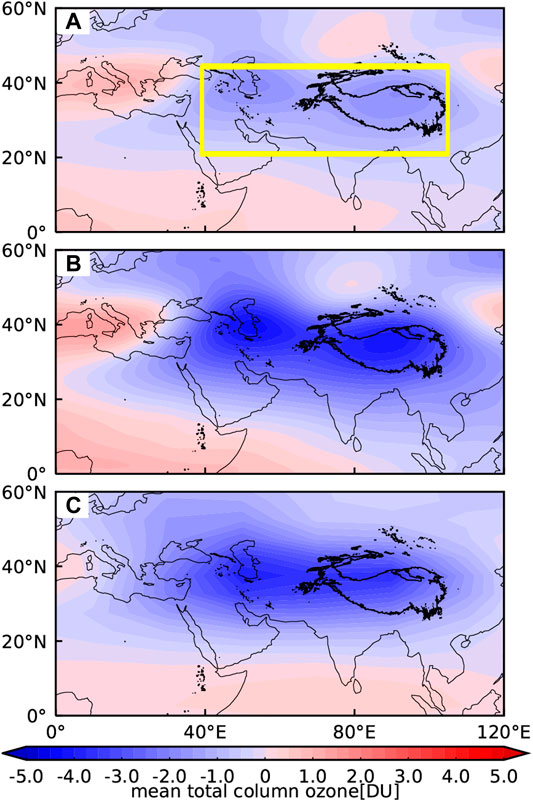
FIGURE 1. The distribution of the TCO* (Unit: DU) averaged from 1984 to 2019 in summer from (A) ERA5, (B) MERRA2, (C) SWOOSH. The bold black contours denote the topography surpassing 3 km. The yellow box outlines the region from 40°E to 105°E and from 20°N to 45°N.
Figure 2 shows the EOF analysis results for the standardized TCO* in summer over the SAH and its adjacent areas. The leading three dominant EOF patterns of the TCO* account for 18.9, 14.8, and 9.8% of the total variance respectively.
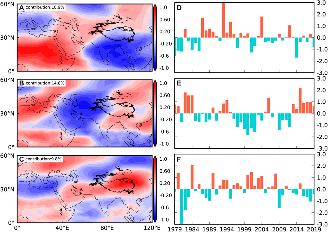
FIGURE 2. The first three EOF patterns of the TCO* from 1979 to 2019 in summer (A–C). The EOF time series (D–F) with the red (blue) bars indicating positive (negative) values. The bold black contours denote the topography surpassing 3 km.
The first dominant EOF pattern of the TCO* (EOF1) exhibits an east-west dipole mode in the low latitude region. It is significantly negative near the south of TP, the Bay of Bengal, the Indochina Peninsula, and the Indian Peninsula in Figure 2A. This EOF1 pattern shifts southwards of the TP into lower latitudes compared to the full pattern in Figure 1.
The EOF2 shows an east-west tripole mode in the middle latitude region and distributes in a smaller scale compared to the EOF1 mode. The prominent negative anomalies over the IP and its surrounding areas (Figure 2B) reflect the local variation over the IP. This EOF2 pattern captures the negative center over the IP in the full TCO* distribution (Figure 1).
The EOF3 shows a south-north mode with a belt-like distribution in the northeast-southwest direction and clear positive anomalies over the eastern part of the TP (Figure 2C). This EOF3 pattern captures the positive center of the eastern part of the TP in the full TCO* distribution. The EOF time series reveal an interannual and interdecadal variation of the TCO* (in Figures 2D–F).
Regression Analysis
Previous studies have revealed that the factors that affect the TCO* over the SAH and its adjacent areas include the geopotential height in the SAH and the height of the tropopause (Zhou et al., 2012; Tang et al., 2019). Based on the EOF analysis, the spatial distribution of the second and third patterns partially reflect the TCO* variations over IP and TP, possibly corresponding to the local tropopause height and the SAH, respectively. To further investigate the relationship between the TCO* and its different affecting factors in summer, regression analysis has been performed.
We first examined the relationship between TCO* and the convective activity, considering the EOF1 (Figure 2A) reflects an east-west dipole mode in the low latitude region. A regression analysis of the outgoing longwave radiation (OLR) field from ERA5 against the EOF time series was conducted, but the results failed a reliability test (figures not shown). We then conducted a regression analysis of SST against the EOF time series (Figure 3), because previous studies have shown that ozone in the UTLS is closely related to the El Niño-Southern Oscillation (ENSO) (Xie et al., 2017; Gamelin et al., 2020). Regression analysis on the first pattern (EOF1) for SST reveals positive anomalies (unit: K) in the middle and east of the equatorial Pacific symmetric about the equator and a region of negative anomalies in the western equatorial Pacific symmetric about the equator. Negative anomalies occur in the tropical southeastern Indian Ocean, while positive anomalies, not significant at the 95% confidence level, occur in the tropical Indian Ocean. This is not surprising as the Indonesian throughflow (ITF) is a critical marine passage that connects the tropical Pacific and Indian Oceans (Yuan et al., 2013). These spatial characteristics are consistent with the Indian Ocean Dipole (IOD) and ENSO teleconnection distribution of the sea surface temperature anomaly (SSTA), indicating that the SSTA is closely related to the TCO* over the SAH and its adjacent areas.
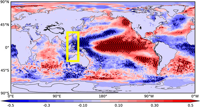
FIGURE 3. Regression analysis of the SST (shading, unit: K) against the time series of EOF1. Black dots indicate the regressed significant SSTs at the 95% confidence level. The bold black contours denote the topography surpassing 3 km. The yellow box outlines the region from 100°E to 120°E and 35°S to 35°N.
Regression analysis on the second and third patterns (EOF2 and EOF3) is not presented as they are not significant at the 95% confidence level in most regions. This is also manifested by the little causal relationship suggested by the information flow analysis of the TCO* and other indices (e.g., IOD index, ENSO index, and Atlantic index). The influence of SST on the EOF2 and EOF3 patterns will be discussed in the following sections.
Figure 4 shows the regression analysis results of the tropopause heights against the EOF time series. The regressed first pattern (Figure 4A) is not significant at the 95% confidence level in the region of the SAH and does not match the EOF1 pattern in Figure 2A, so this pattern is not further investigated. Regression analysis on the second pattern for the tropopause shows negative anomalies (unit: hPa) over the IP significant at the 95% confidence level. Conversely, regression analysis on the third pattern for the tropopause shows positive anomalies (unit: hPa) over the eastern part of the TP significant at the 95% confidence level (Figure 4C), consistent with the south-north mode with obvious positive anomalies over the TP (Figure 2C). These results suggest the abnormally negative tropopause (abnormally high) correlates with abnormally low TCO* and vice versa. Such a correlation can be explained by the relatively lower ozone mass mixing ratio in the upper troposphere than in the lower stratosphere. When the tropopause rises, the lower layer with low ozone contents accounts for more of the ozone mass in the total ozone column, resulting in a lower TCO*.
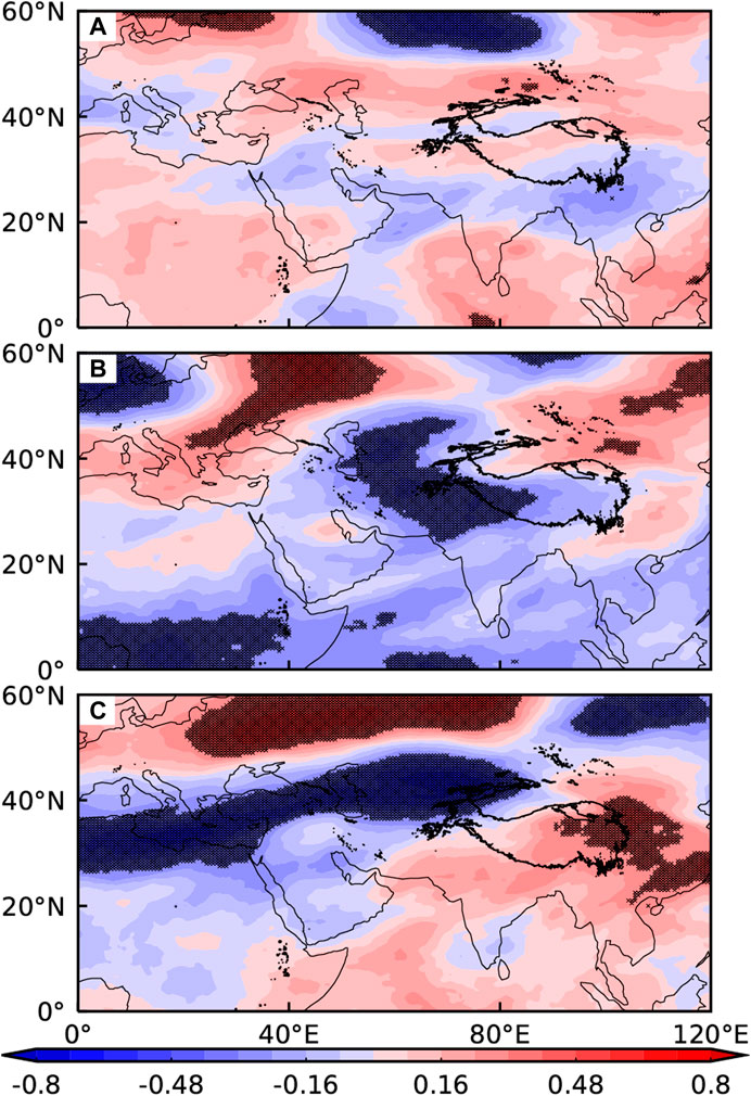
FIGURE 4. Regression analysis of tropopause heights (shading, unit: hPa) against the time series of (A) EOF1, (B) EOF2, and (C) EOF3. Black dots represent the regressed tropopause significant at the 95% confidence level.
Because the tropopause height is related to the strength of the SAH and the TCO* is also related to the geopotential height in the SAH, a regression analysis of the 200 hPa geopotential height against the EOF time series was conducted in the region of the SAH. The regressed first pattern (east-west dipole mode in the low latitudes) is not significant at the 95% confidence level (Figure 5A) and incompatible with the EOF1 pattern in Figure 2A and is thus not further analyzed. Regression analysis on the second pattern for the 200 hPa geopotential height shows positive anomalies (unit: km) over the IP (significant at the 95% confidence level), agreeing well with the clear positive anomalies over the IP revealed by EOF analysis (Figure 2B). This suggests that the divergence strengthens as the SAH becomes abnormally strong, i.e., stronger high-pressure anticyclone. As a result, the abnormal rise of the lower layers with low ozone contents lowers the TCO*.
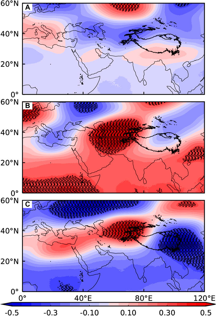
FIGURE 5. Regression analysis of the 200 hPa geopotential height (shading, unit: km) against the time series of (A) EOF1, (B) EOF2, and (C) EOF3. Black dots represent the regressed 200 hPa geopotential height significant at the 95% confidence level.
Regression analysis on the third pattern for the geopotential height shows negative anomalies (significant at the 95% confidence level) over the eastern part of the TP, coincident with the positive anomalies over the eastern part of the TP revealed by EOF analysis (Figure 2C). This indicates the divergence weakens as the SAH becomes abnormally weak i.e., the high-pressure anticyclone is weak, resulting in a weak rise of the lower layers and a higher TCO*. The weakening of the SAH in the eastern region is likely associated with the WPSH as they show synchronous weakening/strengthening (Chen et al., 2011).
Overall, the regression analysis results suggest that the TCO* pattern over the SAH and its adjacent areas in summer is related to three principal components. The east-west dipole mode in low latitudes is mainly related to the SST near Indonesia and the western Pacific Ocean. The east-west tripole mode in the middle latitude region is related to the tropopause height that is closely associated with the strength of the SAH over the IP. The south-north mode is linked to the strength of the SAH, which is likely associated and synchronous with the WPSH. To further understand the function of the three components on the ozone valley, we used the information flow method to determine the causal relationship between the principal components and ozone and then applied a composite analysis to investigate their relations.
The Causal Relation Between the TCO* and Its Principal Components
To determine the causal relationship between the TCO* and the principal components in the same period, we calculated the information flow between the TCO* and the three principal components in summer from 1979 to 2019.
Based on the first regression pattern for SST (shown in Figure 3), the variation of TCO* in the southern area of the TP is closely related to ENSO. However, the information flow between the TCO* and the ENSO index shows little causal relationship in the same period. Considering that TP is geographically far from the middle and east of the equatorial Pacific Ocean, it is reasonable that TCO* and ENSO could hardly affect each other in the same period. Nevertheless, the EOF1 pattern is consistent with the IOD and ENSO teleconnection distribution of SSTA. To evaluate the influence of SST on the first pattern (EOF1), here we define the Indonesia SST index (ISI) as the average SST in the region from 100°E to 120°E and 35°S to 35°N, which locates in the Indonesian throughflow and contains the negative SST anomalies in Indonesia (the yellow box in Figure 3). The information flows between ISI and the TCO* from 1979 to 2019 are given in Figure 6. The information flow is negative in the southern area of the TP, including the eastern and southern parts of the TP, the northern Bay of Bengal, the northern Indochina Peninsula, and the northern Indian Peninsula (Figure 6A). A negative
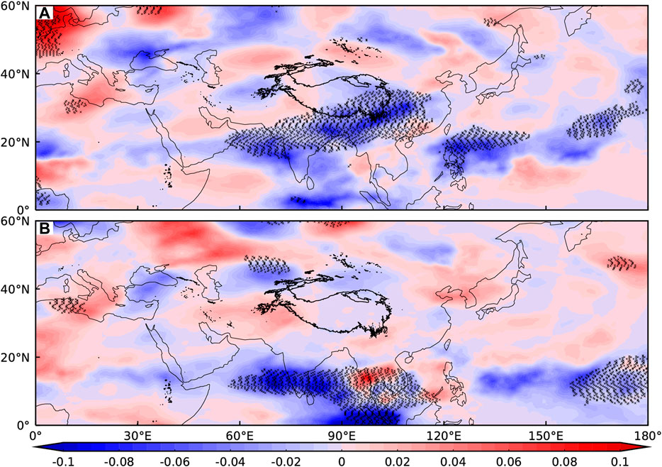
FIGURE 6. Information flow between the Indonesia SST index (ISI) and TCO* (shading). Black dots represent significant information flows at the 90% confidence level; (A)
Similarly, the TCO* variation index (TOI) is defined as the average TCO* in the region from 40°E to 105°E and from 20°N to 45°N, which is the ozone valley over the SAH and its adjacent areas (the yellow box in Figure 1A). The information flow between the tropopause height and the TOI from 1980 to 2019 is given in Figure 7.
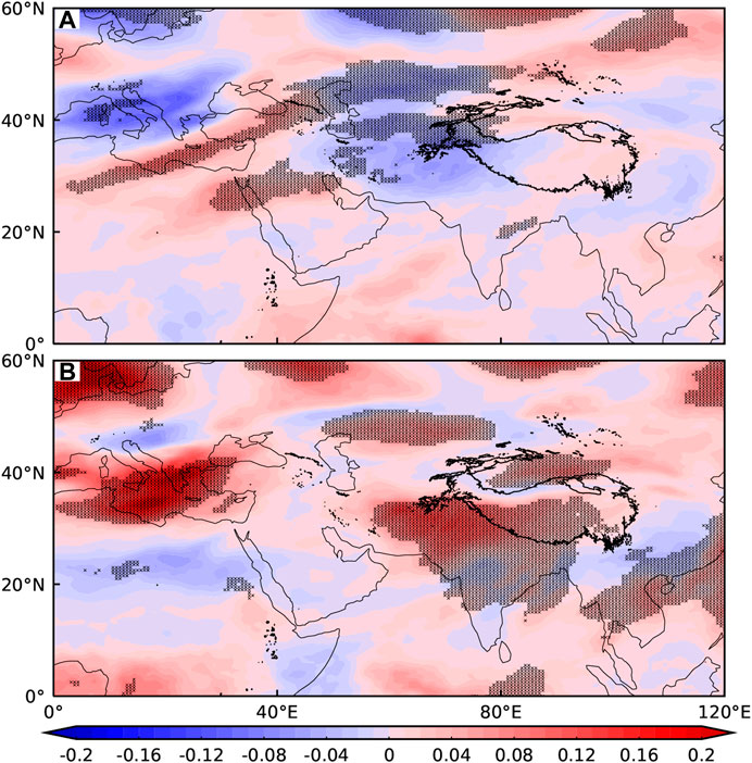
FIGURE 7. Information flow between the tropopause height and the TCO* variation index (TOI) (shading). Black dots represent significant information flows at the 90% confidence level; (A)
Over the western area of the TP, a negative information flow of
The information flow between the 200 hPa geopotential height and the TOI from 1979 to 2019 is shown in Figure 8. Over the IP, the negative information flow of
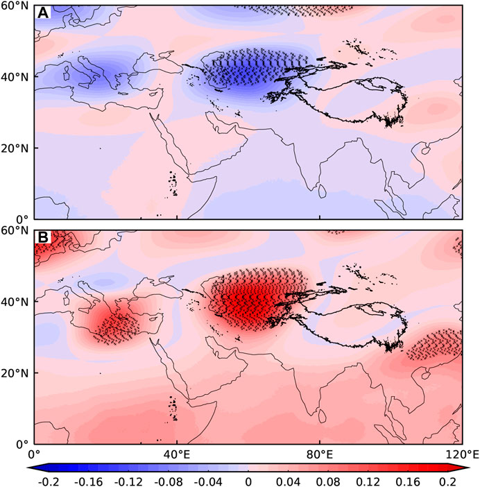
FIGURE 8. Information flow between 200 hPa geopotential height and the TOI (shading). Black dots represent significant information flows at the 90% confidence level; (A)
The information flow between the WPSH index and the TCO* from 1979 to 2019 has been evaluated (Figure 9), because the weakening of the SAH in the eastern region is most likely associated and synchronous with the WPSH as indicated by the regression analysis. Here we focus on the western ridge point index (WRPI) for the WPSH because the information flows between different WPSH indices (including area index, intensity index, ridgeline position, and western ridge point for the WPSH) and the TCO* are similar (figures omitted). The information flow
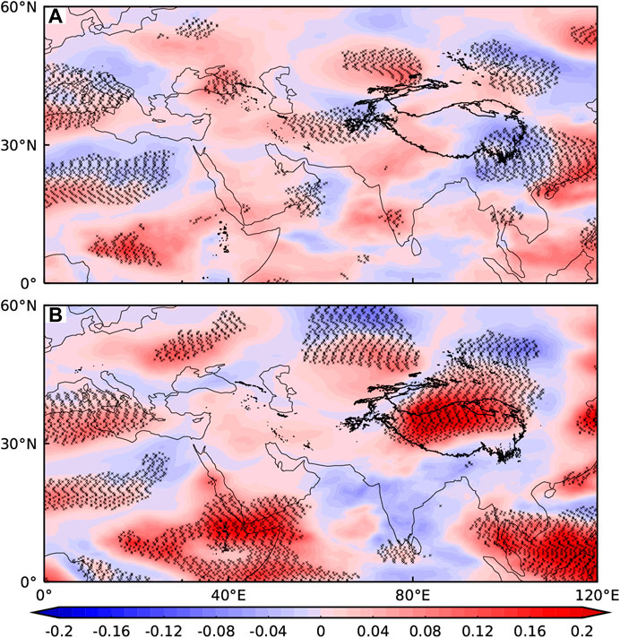
FIGURE 9. Information flow between the western ridge point index (WRPI) for the WPSH and TCO* (shading). Black dots represent significant information flows at the 90% confidence level; (A)
Mechanistic Analysis of the TCO*
Collectively, according to the information flow analysis results, the variation of SST, tropopause height, and the location of WPSH jointly cause the variation of the TCO* over the SAH and its adjacent areas. We applied a composite analysis to analyze the principal components of the TCO* over the SAH and its adjacent areas in summer. Taking an absolute value of the normalized EOF time series of >1 as the standard, individual years with significant positive and negative phases were labeled as stronger and weaker years (Tables 1–3). This information was used in the composite analysis.
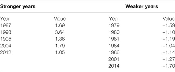
TABLE 1. The stronger and weaker years in the EOF time series 1 and their corresponding time coefficients.
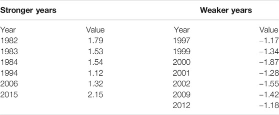
TABLE 2. The stronger and weaker years in the EOF time series 2 and their corresponding time coefficients.
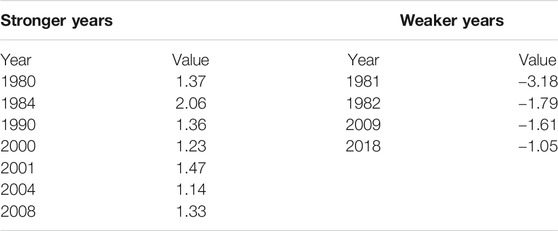
TABLE 3. The stronger and weaker years in the EOF time series 3 and their corresponding time coefficients.
The composite wind field anomalies in the stronger years for EOF time series 1 and SST at 850 and 200 hPa are shown in Figure 10. In the stronger years, the SSTA in the equatorial Central and Eastern Pacific is positive (this area is omitted in Figure 10, but can be seen in Figure 3), while it is negative in the western Pacific. According to the Gill response (i.e., the forced response of atmospheric motion to ocean heat), the cold SSTAs in the warm western Pacific have weakened the zonal SST gradient, which stimulates a series of planetary waves that are transported to the Indian Ocean. As shown in Figure 10A, the SSTA in the western Pacific is negative, and a series of planetary waves symmetric about the equator are transported westwards. A pair of cyclones symmetric about the equator occurs in the yellow areas in Figure 10. Cyclones at low latitudes in the northern hemisphere could intensify anticyclones at higher latitudes, further strengthening the southern trough in the Bay of Bengal, which is formed by currents bypassing the TP (in the green box in Figure 10). In Figure 10B, The composite wind field anomalies at 200 hPa show a pair of anticyclones symmetric about the equator (in the yellow boxes) and an anticyclone over the south of the TP. Comparing the high- and low-level wind fields over the southern TP, it is apparent that with the strengthening of the southern trough at 850 hPa and the strengthening of divergence at 200 hPa, the wind field moves air across the tropopause from the troposphere to the lower stratosphere. Due to the low ozone content in the troposphere, the TCO* in the UTLS decreases. However, during weaker years, it is challenging to identify the divergence at 200 hPa (figures omitted) due to the absence of Gill response. Consequently, the variations of the TCO* are not as apparent as those in the stronger years.
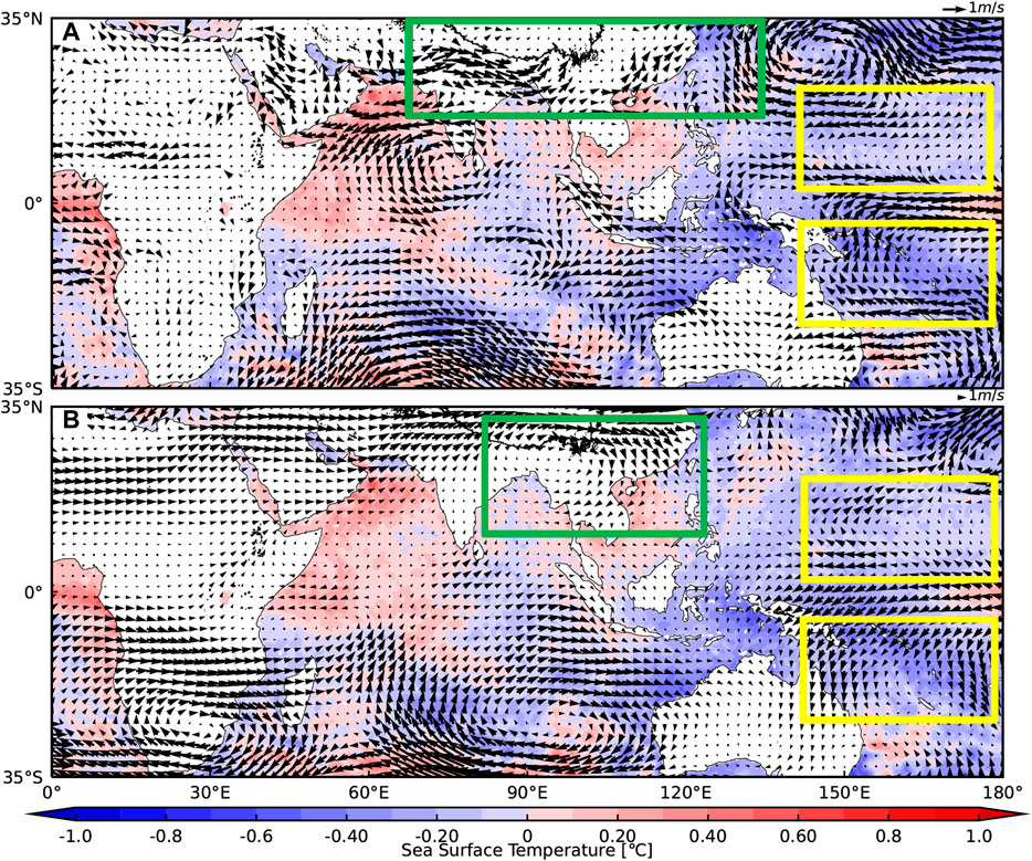
FIGURE 10. Composite wind field in the stronger years for the EOF time series 1 (arrows, unit: m/s) and SST (shading, unit: K) at (A) 850 hPa and (B) 200 hPa.
The composite TCO* and the SAH region for the EOF time series 2 are shown in Figure 11. We took the 12,520 gpm geopotential height isolines to determine the SAH region (Zhang et al., 2000). The location of the SAH remains basically stable, but the TCO* over the IP is closely related to the SAH, showing negative anomalies over the IP for the east-west tripole mode in the middle latitude region. When the SAH is strong over the IP (Figure 11A), the TCO* is correspondingly reduced and the ozone valley’s extent over the IP increases. When the SAH is weak over the IP (Figure 11B), the TCO* over the IP is correspondingly increased and the ozone valley’s extent over the IP decreases.
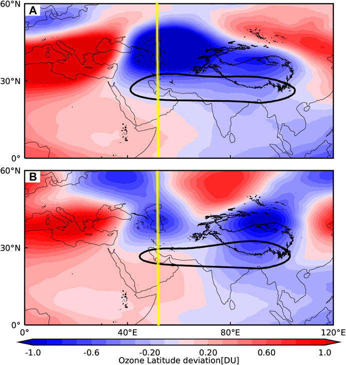
FIGURE 11. The composite TCO* (shading, unit: DU) and the SAH region (solid lines, 12,520 gpm geopotential height isolines) for the EOF time series 2 in the (A) stronger years and (B) weaker years. The yellow lines are the longitude of 50°E.
Figure 11 also shows a large variation in the TCO* along 50°E, and the TCO* over the IP from 35°N to 50°N is negative. The height–latitude cross-sections of the composite wind field along 50°E for the EOF time series 2 are presented in Figure 12. For the stronger years (Figure 12A), from 35°N to 50°N, in the UTLS region, the wind field moves air across the tropopause from the troposphere to the lower stratosphere and is dominated by southerly winds. The low ozone content in the troposphere causes the TCO* in the UTLS decreases. For the weaker years (Figure 12B), the wind field dominated by northerly winds moves from the stratosphere to the troposphere, resulting in the increase of the TCO* in the UTLS.
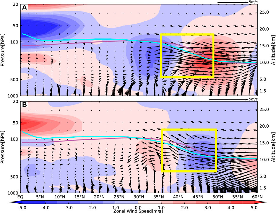
FIGURE 12. The height–latitude cross-sections of the composite wind field (arrows, unit: m/s) along 50°E for the EOF time series 2 in the (A) stronger years and (B) weaker years. The vertical wind speed anomaly is five times of the original wind field. The shadows denote the zonal wind. The purple lines are the heights of the thermal tropopause and the blue lines are the heights of the dynamical tropopause.
The composite TCO* and the SAH region for the EOF time series 3 are shown in Figure 13. Similar to the composites for EOF2, the location of the SAH remains stable, but the TCO* over the TP is closely related to the SAH region, showing the positive anomalies over the TP for the south-north mode. Figure 13A shows that the eastern margin of the SAH could reach 100°E. When the SAH is weak over the TP, the TCO* is correspondingly increased and the ozone valley over the TP decreases. When the SAH is strong over the TP, the eastern region of the SAH could extend to 110°E (Figure 13B) and the TCO* over the TP is correspondingly reduced with an increased extent of the ozone valley over the TP.
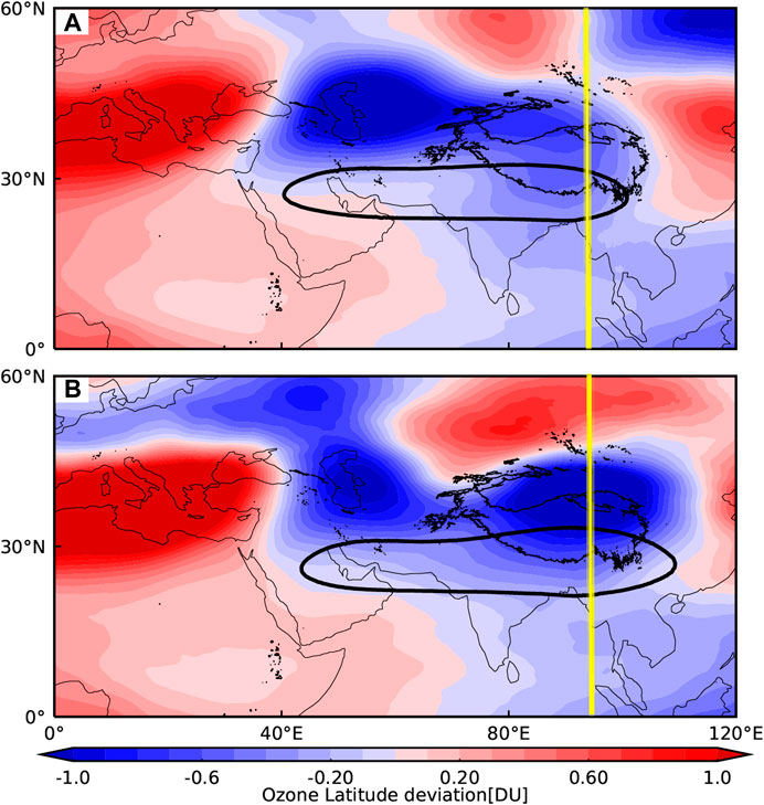
FIGURE 13. The composite TCO* (shading, unit: DU) and the SAH region (solid lines, 12,520 gpm geopotential height isolines) for the EOF time series 3 in the (A) stronger years and (B) weaker years. The yellow lines are the longitude of 95°E.
As the most significant variations are apparent over the TP from 30°N to 45°N (Figure 13), we further analyzed the height–latitude cross-sections of the composite wind field along 95°E for the EOF time series 3 as presented in Figure 14. In Figure 14A, from 30°N to 45°N in the UTLS region, the wind field moves air across the tropopause from the stratosphere with higher ozone content to the troposphere, resulting in increased TCO* in the UTLS region. In contrast, as shown in Figure 14B, the wind field moves air across the tropopause from the troposphere to the lower stratosphere, so the TCO* in the UTLS region decreases.
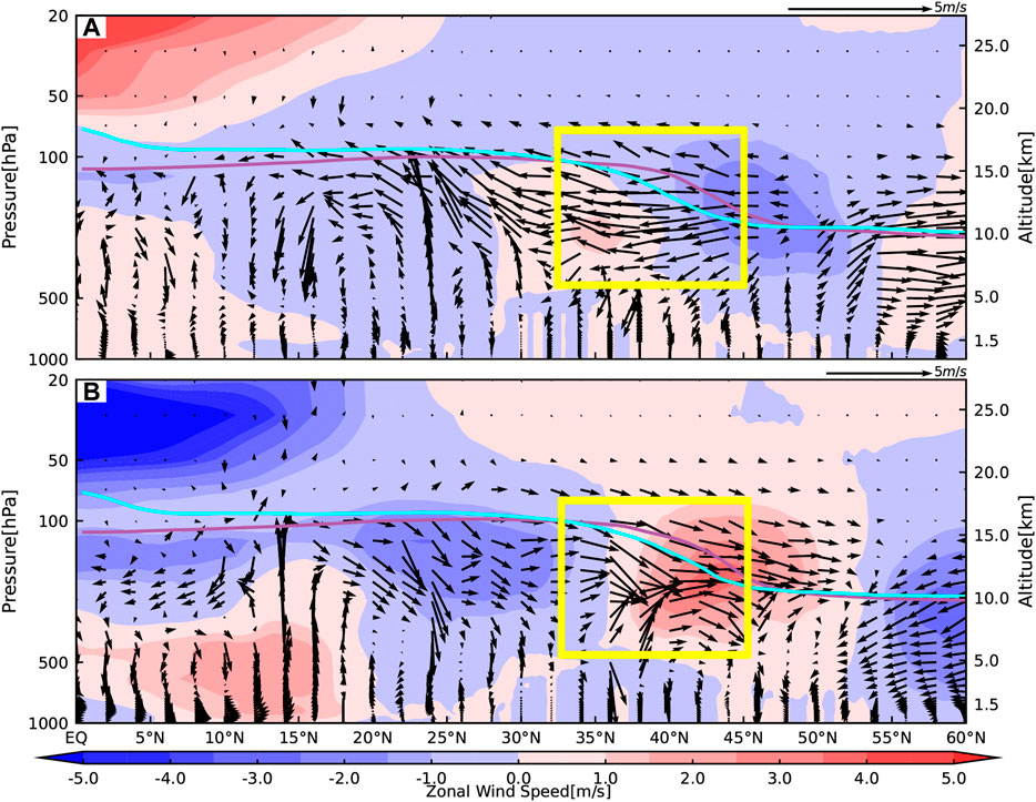
FIGURE 14. The height–latitude cross-sections of the composite wind field (arrows, unit: m/s) along 95°E for the EOF time series 3 in the (A) stronger years and (B) weaker years. Here, the vertical wind speed anomaly is five times of the original wind field. The shadows denote the zonal wind. The purple lines are the height of the thermal tropopause and the blue lines are the height of the dynamical tropopause.
We studied the cause of the positive anomalies over the TP for the south-north mode by analyzing the composite 500 hPa geopotential height (shading, unit: km) for the EOF time series 3 as shown in Figure 15. The most likely cause is the synchronousness between the SAH and the WPSH. When the SAH is weak over the TP, the eastern region of SAH could extend to 100°E (Figure 15A) while the WPSH is relatively weak. When the SAH is strong over the TP, the eastern region of the SAH could extend to 110°E (Figure 15B) while the WPSH is relatively strong (Figure 15B). The TCO* variations in the eastern SAH are therefore related to the location of the WPSH.
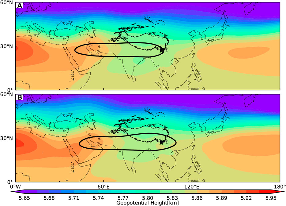
FIGURE 15. The composite 500 hPa geopotential height (shading, unit: km) and the SAH region (solid lines, 12,520 gpm geopotential height isolines) for the EOF time series 3 in the (A) stronger years and (B) weaker years.
Conclusion
Although many factors can affect the variation of the ozone valley, the leading factors have not been determined so far. In our study, the statistical analysis has improved our understanding of the roles of the sea surface temperature (SST), tropopause height, and West Pacific Subtropical High (WPSH) in affecting the ozone valley. Using the ERA5 reanalysis dataset from 1979 to 2019, the MERRA2 reanalysis dataset from 1980 to 2019, and the SWOOSH observation dataset from 1984 to 2019, we examined the individual contribution of each principal component to the summertime ozone valley in the UTLS over the SAH and its adjacent areas. Integrated statistical analysis including the EOF and Liang-Kleeman information flow methods, regression analysis, and composite analysis was applied in the study. The EOF analysis shows that variations of TCO* anomalies have three dominant modes, namely, the east-west dipole mode in the low latitude region (EOF1), the east-west tripole mode in the middle latitude region (EOF2), and the south-north mode (EOF3). The first three EOF patterns of the TCO* account for 18.9, 14.8, and 9.8% of the total variation, respectively.
The regression analysis has revealed the relationship between the TCO* and the principal components in summer. The three leading principal components of TCO* variations are related to 1) the SST near Indonesia and the western Pacific Ocean in low latitudes, 2) the tropopause height over the IP, and 3) the strength of the SAH over the eastern part of the TP, which is linked to the synchronousness between the SAH and the WPSH.
The information flow analysis of the TCO* and the three principal components in summer from 1979 to 2019 helps to determine their causal relationship. The results have shown that the variation of SST, tropopause height, and the location of the WPSH have most likely caused the variation of TCO* over the SAH and its adjacent areas.
For the east-west dipole mode in the low latitude region, composite analysis shows the interaction between the atmosphere and ocean causes the variations of the TCO* in the UTLS near the low latitude region around the TP. For the east-west tripole mode in the middle latitude region, the tropopause over the IP causes the variations of the TCO* in the UTLS. Comparatively, the south-north mode shows the variations of TCO* over the TP are closely related to the location of the WPSH.
In summary, the leading factors affecting the three dominant modes for the variations of the TCO* anomalies are SST, tropopause height, and the WPSH.
Data Availability Statement
The datasets ERA5 for this study can be found in the https://cds.climate.copernicus.eu/#W/home. The datasets MERRA2 can be found in the https://disc.gsfc.nasa.gov/datasets/M2IMNPASM_5.12.4/summary. The datasets SWOOSH can be found in the https://www.esrl.
Author Contributions
The central idea was mainly provided by CS and SC. SC, CS, and DG analyzed the data and analyzed the results. SC prepared the figures. SC and DG wrote the paper. JX contributed to refining the ideas and carrying out additional analyses. All authors contributed to the article and approved the submitted version.
Funding
This work was supported by the National Natural Science Foundation of China (42005063 and 91837311), the Projects (Platforms) for Construction of Top-ranking Disciplines of Guangdong Ocean University (231419022), the National Key R&D Program of China (2018YFA0605604), the project of Enhancing School with Innovation of GuangdongOcean University (230419053), and the Special Funds of Central Finance Support the Development of Local Colleges and Universities of Guangdong Ocean University (000041).
Conflict of Interest
The authors declare that the research was conducted in the absence of any commercial or financial relationships that could be construed as a potential conflict of interest.
Acknowledgments
The authors are grateful to two reviewers for constructive review comments. We thank Zheng Sheng from the National University of Defense Technology for helpful discussions on the results.
Supplementary Material
The Supplementary Material for this article can be found online at: https://www.frontiersin.org/articles/10.3389/feart.2020.605703/full#supplementary-material.
References
Bian, J., Yan, R., Chen, H., Lü, D., and Massie, S. T. (2011). Formation of the summertime ozone valley over the Tibetan Plateau: the Asian summer monsoon and air column variations. Adv. Atmos. Sci. 28 (6), 1318–1325. doi:10.1007/s00376-011-0174-9
Cagnazzo, C., Claud, C., and Hare, S. (2006). Aspects of stratospheric long-term changes induced by ozone depletion. Clim. Dynam. 27 (1), 101–111. doi:10.1007/s00382-006-0120-1
Chang, S., Sheng, Z., Du, H., Ge, W., and Zhang, W. (2020a). A channel selection method for hyperspectral atmospheric infrared sounders based on layering. Atmos. Meas. Tech. 13 (2), 629–644. doi:10.5194/amt-13-629-2020
Chang, S., Sheng, Z., Zhu, Y., Shi, W., and Luo, Z. (2020b). Response of ozone to a gravity wave process in the UTLS region over the Tibetan Plateau. Front. Earth Sci. 8, 289. doi:10.3389/feart.2020.00289
Chen, Y., Li, Y., and Qi, D. (2011). Variations of south Asia high and west pacific subtropical high and their relationships with precipitation. Plateau Meteorol. 30 (5), 1148–1157. doi:10.1007/s00376-010-1000-5
Chipperfield, M. P., Bekki, S., Dhomse, S., Harris, N. R. P., Hassler, B., Hossaini, R., et al. (2017). Detecting recovery of the stratospheric ozone layer. Nature 549 (7671), 211–218. doi:10.1038/nature23681
Crutzen, P. J. (1970). The influence of nitrogen oxides on the atmospheric ozone content. Q. J. R. Meteorol. Soc. 96 (408), 320–325. doi:10.1002/qj.49709640815
Das, S. S., Suneeth, K. V., Ratnam, M. V., Girach, I. A., and Das, S. K. (2019). Upper tropospheric ozone transport from the sub-tropics to tropics over the Indian region during Asian summer monsoon. Clim. Dynam. 52 (7–8), 4567–4581. doi:10.1007/s00382-018-4418-6
Gamelin, B. L., Carvalho, L. M. V., and Kayano, M. (2020). The combined influence of ENSO and PDO on the spring UTLS ozone variability in South America. Clim. Dynam. 55, 1539–1562. doi:10.1007/s00382-020-05340-0
Gonzalez, P. L. M., Polvani, L. M., Seager, R., and Correa, G. J. P. (2014). Stratospheric ozone depletion: a key driver of recent precipitation trends in South Eastern South America. Clim. Dynam. 42 (7–8), 1775–1792. doi:10.1007/s00382-013-1777-x
Guo, D., Su, Y., Shi, C., Xu, J., and Powell, A. M. (2015). Double core of ozone valley over the Tibetan Plateau and its possible mechanisms. J. Atmos. Sol. Terr. Phys. 130, 127–131. doi:10.1016/j.jastp.2015.05.018
Guo, D., Xu, J., Su, Y., Shi, C., Liu, Y., and Li, W. (2017). Comparison of vertical structure and formation mechanism of summer ozone valley over the Tibetan Plateau and North America. Trans. Atmos. Sci. 40 (3), 412–417. doi:10.13878/j.cnki.dqkxxb.20160315001
He, Y., Sheng, Z., and He, M. (2020). The first observation of turbulence in Northwestern China by a near-space. high-resolution balloon sensor. Sensors 20 (3), 677. doi:10.3390/s20030677
Li, Z., Qin, H., Guo, D., Zhou, S., Huang, Y., Su, Y., et al. (2017). Impact of ozone valley over the Tibetan Plateau on the South Asian high in CAM5. Adv. Meteorol. 2017, 1–8. doi:10.1155/2017/9383495
Liang, X. S. (2013). The Liang-Kleeman information flow: theory and applications. Entropy. 15 (1), 327–360. doi:10.3390/e15010327
Liang, X. S. (2014). Unraveling the cause-effect relation between time series. Phys. Rev. E – Stat. Nonlinear Soft Matter Phys. 90 (5), 052150. doi:10.1103/PhysRevE.90.052150
Mai, Y., Sheng, Z., Shi, H., Liao, Q., and Zhang, W. (2020). Spatiotemporal distribution of atmospheric ducts in Alaska and its relationship with the Arctic vortex. Int. J. Antenn. Propag. 2020, 1–13. doi:10.1155/2020/9673289
Mohanakumar, K., Raghavan, S. K., Pezholil, M., Vasudevan, K., Manoj, M. G., Samson, T., et al. (2018). A versatile 205 MHz stratosphere-troposphere radar at Cochin–scientific applications. Curr. Sci. 114, 2459–2466. doi:10.18520/cs/v114/i12/2459-2466
Molina, M. J., and Rowland, F. S. (1974). Stratospheric sink for chlorofluoromethanes: chlorine atom-catalysed destruction of ozone. Nature 249 (5460), 810–812. doi:10.1038/249810a0
Pan, L. L., Homeyer, C. R., Honomichl, S., Ridley, B. A., Weisman, M., Barth, M. C., et al. (2014). Thunderstorms enhance tropospheric ozone by wrapping and shedding stratospheric air. Geophys. Res. Lett. 41 (22), 7785–7790. doi:10.1002/2014gl061921
Peters, D. H. W., Schneidereit, A., Bugelmayer, M., Zuelicke, C., and Kirchner, I. (2015). Atmospheric circulation changes in response to an observed stratospheric zonal ozone anomaly. Atmos.-Ocean 53 (1), 74–88. doi:10.1080/07055900.2013.878833
Randel, W. J., Polvani, L., Wu, F., Kinnison, D. E., Zou, C.-Z., and Mears, C. (2017). Troposphere-stratosphere temperature trends derived from satellite data compared with ensemble simulations from WACCM. J. Geophys. Res. -Atmos 122 (18), 9651–9667. doi:10.1002/2017jd027158
Shi, C., Zhang, C., and Guo, D. (2017). Comparison of electrochemical concentration cell ozonesonde and microwave limb sounder satellite remote sensing ozone profiles for the center of the South Asian High. Rem. Sens. 9 (10), 1012. doi:10.3390/rs9101012
Shi, G., Bai, Y., Y, I., and Ohashi, T. (2000). A balloon measurement of the ozone vertical distribution over Lahsa. Adv. Earth Sci. 15 (5), 522–524. doi:10.11867/j.issn.1001-8166.2000.05.0522
Stolarski, R. S., Waugh, D. W., Wang, L., Oman, L. D., Douglass, A. R., and Newman, P. A. (2014). Seasonal variation of ozone in the tropical lower stratosphere: southern tropics are different from northern tropics. J. Geophys. Res. -Atmos 119 (10), 6196–6206. doi:10.1002/2013jd021294
Tang, Z., Guo, D., Su, Y., Shi, C., Zhang, C., Liu, Y., et al. (2019). Double cores of the Ozone Low in the vertical direction over the Asian continent in satellite data sets. Earth Planet. Phys. 3 (2), 93–101. doi:10.26464/epp2019011
Tian, W., Chipperfield, M., and Huang, Q. (2008). Effects of the Tibetan Plateau on total column ozone distribution. Tellus B. 60 (4), 622–635. doi:10.1111/j.1600-0889.2008.00338.x
Tobo, Y., Iwasaka, Y., Zhang, D., Shi, G., Kim, Y.-S., Tamura, K., et al. (2008). Summertime “ozone valley” over the Tibetan Plateau derived from ozonesondes and EP/TOMS data. Geophys. Res. Lett. 35 (16), L16801. doi:10.1029/2008GL034341
Wargan, K., Labow, G., Frith, S., Pawson, S., Livesey, N., and Partyka, G. (2017). Evaluation of the ozone fields in NASA’s MERRA-2 reanalysis. J. Clim. 30 (8), 2961–2988. doi:10.1175/jcli-d-16-0699.1
WMO (2011). Report No.: 516. Scientific assessment of ozone depletion: global ozone research and monitoring project. Geneva, Switzerland: World Meteorological Organization.
Xia, Y., Huang, Y., and Hu, Y. (2018). On the climate impacts of upper tropospheric and lower stratospheric ozone. J. Geophys. Res.: Atmos. 123 (2), 730–739. doi:10.1002/2017jd027398
Xie, F., Li, J., Zhang, J., Tian, W., Hu, Y., Zhao, S., et al. (2017). Variations in North Pacific sea surface temperature caused by Arctic stratospheric ozone anomalies. Environ. Res. Lett. 12 (11). 114023. doi:10.1088/1748-9326/aa9005
Yu, Y., and Ren, R. (2019). Understanding the variation of stratosphere-troposphere coupling during stratospheric northern annular mode events from a mass circulation perspective. Clim. Dynam. 53 (9–10), 5141–5164. doi:10.1007/s00382-019-04675-7
Yuan, D., Zhou, H., and Zhao, X. (2013). Interannual climate variability over the tropical pacific ocean induced by the Indian Ocean Dipole through the Indonesian throughflow. J. Clim. 26 (9), 2845–2861. doi:10.1175/JCLI-D-12-00117.1
Zhang, J., Tian, W., Xie, F., Sang, W., Guo, D., Chipperfield, M., et al. (2019). Zonally asymmetric trends of winter total column ozone in the northern middle latitudes. Clim. Dynam. 52 (7–8), 4483–4500. doi:10.1007/s00382-018-4393-y
Zhang, J., Tian, W., Xie, F., Tian, H., Luo, J., Zhang, J., et al. (2014). Climate warming and decreasing total column ozone over the Tibetan Plateau during winter and spring. Tellus Ser. B Chem. Phys. Meteorol. 66 (1), 1–12. doi:10.3402/tellusb.v66.23415
Zhang, Q., Qian, Y., and Zhang, X. (2000). Interannual and interdecadal variations of the south Asia high. Sci. Atmos. Sin. 24 (1), 67–78. doi:10.3878/j.issn.1006-9895.1401.13221
Zhou, S., Yang, S., Zhang, R., Li, H., and Meirong, W. (2012). Possible causes of total ozone depletion over the Qinghai-Xizang plateau and its relation to tropopause height in recent 30 years. Plateau Meteorol. 31 (6), 1471–1478. doi:10.1007/s11783-011-0280-z
Zhou, X., Li, W., Chen, L., and Liu, Y. (2004). Study of ozone change over Tibetan Plateau. Acta Meteorol. Sin. 5, 513–527. doi:10.1029/96GL00767
Keywords: ozone valley, upper troposphere and lower stratosphere, South Asian High, empirical orthogonal function, Liang-Kleeman information flow
Citation: Chang S, Shi C, Guo D and Xu J (2021) Attribution of the Principal Components of the Summertime Ozone Valley in the Upper Troposphere and Lower Stratosphere. Front. Earth Sci. 8:605703. doi: 10.3389/feart.2020.605703
Received: 13 September 2020; Accepted: 21 December 2020;
Published: 22 January 2021.
Edited by:
Chaim Garfinkel, Hebrew University of Jerusalem, IsraelReviewed by:
Lin Wang, Institute of Atmospheric Physics (CAS), ChinaEric Ray, National Oceanic and Atmospheric Administration, United States
Copyright © 2021 Chang, Shi, Guo and Xu. This is an open-access article distributed under the terms of the Creative Commons Attribution License (CC BY). The use, distribution or reproduction in other forums is permitted, provided the original author(s) and the copyright owner(s) are credited and that the original publication in this journal is cited, in accordance with accepted academic practice. No use, distribution or reproduction is permitted which does not comply with these terms.
*Correspondence: Dong Guo, ZG9uZ2d1b0BudWlzdC5lZHUuY24=