 Yota Sato1*
 Koji Fujita1
 Hiroshi Inoue2
 Sojiro Sunako3
 Akiko Sakai1Akane Tsushima1,4†
 Evgeny A. Podolskiy5,6
 Rakesh Kayastha7
 Rijan B. Kayastha7
- 1Graduate School of Environmental Studies, Nagoya University, Nagoya, Japan
- 2National Research Institute for Earth Science and Disaster Resilience (NIED), Tsukuba, Japan
- 3Snow and Ice Research Center, National Research Institute for Earth Science and Disaster Resilience (NIED), Nagaoka, Japan
- 4Japan Meteorological Agency, Meteorological Research Institute, Tsukuba, Japan
- 5Arctic Research Center, Hokkaido University, Sapporo, Japan
- 6Global Station for Arctic Research, Global Institution for Collaborative Research and Education, Hokkaido University, Sapporo, Japan
- 7Himalayan Cryosphere, Climate, and Disaster Research Center (HiCCDRC), Department of Environmental Science and Engineering, School of Science, Kathmandu University, Dhulikhel, Nepal
Ice cliffs can act as “hot spots” for melt on debris-covered glaciers and promote local glacier mass loss. Repeat high-resolution remote-sensing data are therefore required to monitor the role of ice cliff dynamics in glacier mass loss. Here we analyze high-resolution aerial photogrammetry data acquired during the 2007, 2018, and 2019 post-monsoon seasons to delineate and monitor the morphology, distribution, and temporal changes of the ice cliffs across the debris-covered Trakarding Glacier in the eastern Nepal Himalaya. We generate an ice cliff inventory from the 2018 and 2019 precise terrain data, with ice cliffs accounting for 4.7 and 6.1% of the debris-covered area, respectively. We observe large surface lowering (>2.0 m a−1) where there is a denser distribution of ice cliffs. We also track the survival, formation, and disappearance of ice cliffs from 2018 to 2019, and find that ∼15% of the total ice cliff area is replaced by new ice cliffs. Furthermore, we observe the overall predominance of northwest-facing ice cliffs, although we do observe spatial heterogeneities in the aspect variance of the ice cliffs (ice cliffs face in similar/various directions). Many new ice cliffs formed across the stagnant middle sections of the glacier, coincident with surface water drainage and englacial conduit intake observations. This spatial relationship between ice cliffs and the glacier hydrological system suggests that these englacial and supraglacial hydrological systems play a significant role in ice cliff formation.
Introduction
Glaciers in High Mountain Asia have been shrinking in recent decades (e.g., Bolch et al., 2012; Brun et al., 2017; Shean et al., 2020). Around 10–19% of the glacier area in High Mountain Asia is debris-covered (Herreid and Pellicciotti, 2020), with this debris cover contributing to complex melting processes (e.g., Zhang et al., 2011). A debris mantle thicker than ∼5 cm has an insulating effect, whereas a debris layer that is only a few centimeters thick can enhance ice ablation (e.g., Mattson et al., 1993; Østrem, 1959; Nicholson and Benn, 2006). Conversely, several studies have revealed that debris-covered and clean glaciers possess comparable thinning rates (e.g., Kääb et al., 2012; Nuimura et al., 2012; Gardelle et al., 2013; Lamsal et al., 2017; Brun et al., 2019), and have called this phenomenon a “debris-covered anomaly” (Pellicciotti et al., 2015; Vincent et al., 2016; Salerno et al., 2017). It has been suggested that the local facilitation of debris-cover-driven glacier melting can be caused by ice cliffs and ponds, which are considered “hotspots” of melt (e.g., Sakai et al., 1998; Sakai et al., 2002; Han et al., 2010; Steiner et al., 2015; Buri et al., 2016; Thompson et al., 2016; Brun et al., 2018; Anderson et al., 2019a).
Several ice cliff studies have analyzed field observations and employed remote-sensing methods to elucidate ice cliff processes. Sakai et al. (1998) first observed the ice cliff backwasting rate across Lirung Glacier, Nepal. Subsequent studies have attempted to quantify the amount of ice cliff ablation using high-resolution remote-sensing data. Thompson et al. (2016) computed the thinning rate of Ngozumpa Glacier, Khumbu region, Nepal, using high-resolution (1.0 m) digital elevation models (DEMs), and found that ice cliff wasting contributed to ∼40% of the total surface lowering, even though ice cliffs occupied only 5% of the total debris-covered area. Recent developments in photogrammetry-based terrain data processing and unmanned aerial vehicle (UAV) technology have greatly advanced ice cliff research (e.g., Immerzeel et al., 2014). Brun et al. (2018) combined in situ measurements, UAV photogrammetry, and satellite data to estimate the ice cliff mass loss across the debris-covered area of the Changri Nup Glacier in the Khumbu region, Nepal. They estimated that ice cliff ablation contributed to ∼23% of the total glacier mass loss, even though the ice cliff area accounted for only ∼8% of the debris-covered area. Studies on the spatial distribution and temporal changes of ice cliffs have also been conducted at the regional scale to elucidate ice cliff processes. Watson et al. (2017a) extracted ice cliffs and supraglacial ponds across 14 glaciers in the Khumbu region, Nepal, using Google Earth Pro, and found that the ice cliffs were primarily north-facing, regardless of the glacier-flow direction, with supraglacial ponds often forming adjacent to the ice cliffs. Steiner et al. (2019) analyzed the spatiotemporal variability of ice cliffs during the 1974–2015 period by combining multiple satellite images in the Langtang catchment of Nepal, and revealed that 17% of the ice cliffs at the Langtang Glacier have persisted for nearly a decade.
Only a few high-resolution (decimeter scale) annual ice cliff monitoring studies have been conducted to date, although these previous studies have extended our understanding of ice cliff processes on debris-covered glaciers (e.g., Immerzeel et al., 2014; Brun et al., 2018). Therefore, the morphology (i.e., size, slope, and aspect), spatial distribution, and dynamics (formation and decay processes) of ice cliffs across debris-covered glaciers remain largely unknown. Here we employ high-resolution photogrammetry to (1) generate an ice cliff inventory, (2) characterize the morphology and spatial distribution of ice cliffs, and (3) observe ice cliff persistence, decay, and formation at the annual scale across the debris-covered Trakarding Glacier in the eastern Nepal Himalaya.
Study Site, Data, and Methods
Study Site
Debris-covered Trakarding Glacier (27.9°N, 86.5°E) is located in Rolwaling Valley in the eastern Nepal Himalaya (Figure 1A,B); the debris-free Trambau Glacier is situated above (Sunako et al., 2019), and has been disconnected from Trakarding Glacier since the 1970s. Previous studies have treated the two glaciers as the “Trakarding–Trambau Glacier system” (Podolskiy et al., 2018; Podolskiy et al., 2019; Sunako et al., 2019). The total area of the system is 31.7 km2 (Nuimura et al., 2015), and spans elevations of 4,500–6,690 m above sea level (a.s.l.). Trakarding Glacier is surrounded by steep valley sides, with snow accumulation occurring largely through avalanches from the eastern headwall (Sunako et al., 2019). A negative mass balance has been confirmed via stake measurements (Sunako et al., 2019). It is a lake-terminating glacier, with Tsho Rolpa, one of the largest glacial lakes in Nepal, at its terminus. Tsho Rolpa has been expanding since the 1950s (Sakai et al., 2000a; Fujita et al., 2013). Trakarding Glacier has a debris-covered area of 2.9 km2 and extends 4.7 km along the glacier centerline, with flow to the northwest (∼310°), based on its 2018 terminus position. We have divided the study area into nine sections, labeled sections A–I (500 m intervals from the 2018 terminus), to analyze the spatial characteristics of the ice cliff distribution (Figure 1C).
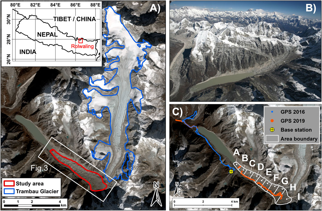
FIGURE 1. Details of the study area. (A) Location of the Rolwaling region and overview of the Trakarding-Trambau Glacier system. (B) Aerial photograph of the study area, taken from a business jet plane during the photogrammetry survey on November 24, 2007. (C) Outline of the study section boundaries along the debris-covered Trakarding Glacier and GPS tracks. The white box in (A) denotes the domain of Figure 3. The background image in (A) and (C) is a Sentinel-2 satellite image (acquired on November 24, 2017). Glacier boundaries are modified from the GAMDAM Glacier Inventory (Nuimura et al., 2015; Sakai, 2019).
Field Observations
We have conducted five field campaigns across Trakarding Glacier since 2016. We first deployed mass-balance stakes across the glacier in May 2016, which have been resurveyed every October from 2016 to 2019. The stake positions were measured using a differential global positioning system (DGPS, GEM-1/-2, Enabler Inc.). We also conducted a kinematic DGPS survey across both the on- and off-glacier terrain in May 2016 and October to November 2019 to obtain validation points for the photogrammetry-based DEMs (Figure 1C). The base station for this survey was installed beside the automatic weather station at 4,806 m a.s.l. on the lateral moraine (Figure 1C).
Aerial Photogrammetry Survey
We used three aerial photogrammetry datasets to monitor the surface elevation changes, surface flow velocity, and ice cliff distribution across the debris-covered area of Trakarding Glacier (Table 1). We conducted two of the photogrammetry surveys during the 2018 and 2019 field campaigns; we also analyzed the data from a 2007 photogrammetry survey to identify any decadal-scale changes. We chartered a helicopter on October 18, 2018, and mounted three cameras (Richo GR and GRII) on the skid and lower pilot’s window (Supplementary Figure S1A), with images acquired at a 2-s interval. We then mounted a Richo GRII camera (1-s interval time-lapse mode setting) onto a fixed-wing UAV (Hobbyking Sky Walker X-5; Supplementary Figure S1B), which had a 1.8 m wingspan and 1.4 kg body (including camera), for four flights on 18 and October 19, 2019. The mean flight speed was ∼60 km h−1, with a maximum flight time of ∼60 min. The UAV details are available in Fujita et al. (2017). The flight path was set to obtain an alongside overlap of ∼80%, side overlap of ∼60%, and <0.2 m ground resolution.
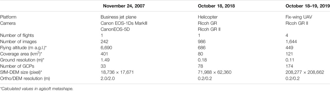
TABLE 1. Details of the aerial photogrammetry survey and structure from motion data processing.
We analyzed the aerial photogrammetry dataset taken from a private jet in 2007 (Figure 1B) to estimate the decadal change in debris-covered area. The flight altitude was estimated as ∼6,700 m above ground level (a.g.l.; Table 1), and Canon EOS-5D and Canon EOS-1Ds cameras were used for the image acquisition. However, the ground resolution was rather coarse due to the high flight altitude, such that delineation of the ice cliffs and supraglacial ponds was not possible. Therefore, these data were only used for our surface elevation change analysis. We successfully obtained images of the off-glacier terrain in 2007 and 2018, whereas the 2019 images mainly covered the main body of Trakarding Glacier, with limited off-glacier terrain coverage (Supplementary Figure S2).
Ground Control Points
We extracted ground control points (GCPs) for the photogrammetry data processing (Structure From Motion Data Processing) using ortho-images and a DEM derived from the Pléiades satellite imagery. The Pléiades image was acquired on December 1, 2017. The ortho-image and DEM resolutions are 0.5 and 2.0 m, respectively (Berthier et al., 2014). We assessed the vertical accuracy of the Pléiades-derived DEM (hereafter Pléiades-DEM) using in-situ DGPS measurements obtained at off-glacier sites in 2016. The GPS data points that were acquired during the 2016 field campaign were projected to Universal Transverse Mercator coordinates (UTM, zone 45 north, WGS84). The GPS points were then interpolated in ArcGIS using the inverse distance weighted method to create a GPS-derived DEM (hereafter GPS-DEM) with the same grid size as the Pléiades-DEM. Grid cells with no GPS points were then excluded (Tshering and Fujita, 2016).
Berthier et al. (2014) reported that the vertical accuracy of Pléiades-DEMs can be improved by shifting the DEMs horizontally. The elevation difference relative to the GPS-DEM was calculated by shifting the Pléiades-DEM horizontally in 0.5 m increments (one pixel of the Pléiades panchromatic ortho-image). We estimated the most suitable shifting position that minimized the standard deviation (SD) of the elevation difference between the Pléiades- and GPS-DEMs (Berthier et al., 2007). Grid cells containing surface slopes steeper than 30° were not used for the accuracy assessment (Fujita et al., 2008; Nuimura et al., 2012). The minimum SD of the elevation difference (0.97 m) was found when the Pléiades-DEM was shifted horizontally by +3.5 m in the easting direction and −3.0 m in the northing direction (N = 17,047 GPS-DEM grid cells). The mean vertical residual (0.88 m) was then corrected after the Pléiades-DEM shift. The GCPs were extracted (locations and elevations) from the panchromatic ortho-image after the Pléiades-DEM shift, which also shifted with the DEM. The topographic features (e.g., boulders or rock cracks) of these GCPs were located on the stable off-glacier terrain.
Structure From Motion Data Processing
Structure from Motion (SfM) was used to generate ortho-images and DEMs from the aerial photographs. We used Agisoft Metashape Professional Edition 1.5.1 (Agisoft LLC, 2020) for the data processing, and followed the analysis workflow outlined in Lucieer et al. (2014), Wigmore and Mark (2017), and the Agisoft Metashape Professional User manual (2020). We initially focused on the 2018 photogrammetry dataset since the aerial photogrammetry coverage area in 2018 extended to the off-glacier terrain; we extracted 78 GCPs from the shifted Pléiades-DEM and ortho-image (Ground Control Points) to create the 2018 ortho-image and DEM (hereafter SfM-DEM-2018). We corrected the SfM-DEM-2018 by the mean elevation difference relative to the GPS-DEM. We further extracted GCPs on the off-glacier terrain from the SfM-DEM/ortho-image-2018 and used these GCPs for the other photogrammetry datasets. The SfM data processing workflow is shown in Figure 2A, and the GCP locations are shown in Supplementary Figure S2. The SfM-DEM vertical biases (mean elevation difference ± SD) relative to the GPS-DEMs were 1.21 ± 2.32 m (2007), −1.58 ± 1.82 m (2018), and 4.64 ± 2.35 m (2019; Table 2; Supplementary Figure S3). Each SfM-DEM bias was corrected using these mean elevation differences. We could not compute the stable-ground elevation differences because the UAV photogrammetry area obtained in 2019 was spatially limited. Therefore, we estimated the relative GCP vertical error (Supplementary Table S1) and GCP placement error that was calculated in Agisoft Metashape (Supplementary Table S2) for additional error assessments.
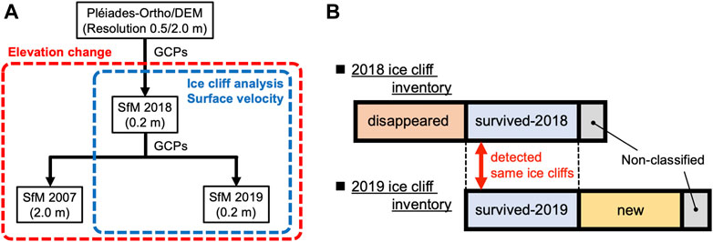
FIGURE 2. (A) Structure from Motion data processing workflow and (B) conceptual diagram of the ice cliff annual tracking and classification.
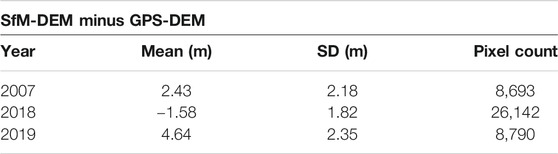
TABLE 2. Accuracy of the SfM-DEMs.
Ice Cliff Analysis
Delineation
We delineated the ice cliffs on the debris-covered area to characterize the ice cliff morphology and spatial distribution. The ortho-image and processed SfM-DEM data (hillshade, aspect, and slope) were analyzed in ArcGIS, with edge polylines and slope polygons manually created on the ridges and slope sections of the ice cliffs, respectively (Supplementary Figure S4). We calculated the ridge length, ice cliff height, mean slope of the cells within each ice cliff polygon, horizontal footprint of the slope (map-view area), ice cliff inclined area (actual slope area; Supplementary Figure S4E), and ice cliff orientation, which is the vector mean of all of the grid cells contained in the slope polygons, from the ice cliff inventory. We also delineated the supraglacial ponds on the debris-covered area and analyzed their spatial adjacency with ice cliffs by checking the relative positions of the ponds and cliffs polygons in the ArcGIS environment.
One main operator (researcher) delineated all of the ice cliffs to ensure that the ice cliffs were selected and delineated in a consistent manner. We then evaluated the delineated ice cliffs independently to estimate the delineation uncertainty due to subjective bias. Specifically, five operators (including the main operator) generated ridge lines and slope polygons for 20 randomly selected ice cliffs of various size and shape. We then calculated the standard deviations of the edge length and map-view area for these 20 ice cliffs. The ice cliff inclined area is strongly affected by the cliff slope, which depends on the DEM quality. Therefore, we also tested the inclined area’s sensitivity to a slope angle change of ±1° for all of the ice cliffs.
The ice cliff inclined area strongly relates to mass loss; therefore, we defined “ice cliff density (m2 m−2)” as an indicator of the spatial density of ice cliffs. The total ice cliff inclined area in each section was divided by the section map-view area. We also estimated the ice cliff length density, which is defined as the ice cliff edge length per square meter, for comparison with a previous study in the neighboring Khumbu region (Watson et al., 2017a). We calculated the circular variance of the ice cliff orientation (Fisher, 1995), which is defined by the following equation:
where
where
Tracking Temporal Changes in Ice Cliffs
We tracked the evolution, persistence, and decay of ice cliffs by comparing the 2018 and 2019 ice cliff inventories. Figure 2B shows ice cliff classification, whereby the ice cliffs are defined as either “survived”, “new”, or “disappeared”. The survived-2018 and -2019 cliffs are those that have been identified in both inventories. Conversely, the new cliffs are those in the 2019 inventory that could not be detected in the 2018 inventory, and the disappeared cliffs are those in the 2018 inventory that could not be detected in the 2019 inventory. Some survived-2018 ice cliffs either merged or split after one year, resulting in slight variations between the number of survived cliffs in 2018 and 2019. We defined the remaining ice cliffs that could not be clearly categorized as “non-classified” cliffs.
Surface Elevation Change, Surface Flow Velocity, and Water Flow Analyses
We estimated the decadal (2007–2018) and annual (2018–2019) surface elevation changes of the debris-covered area by differentiating the generated SfM-DEMs. We modified the glacier area from the GAMDAM Glacier Inventory (Nuimura et al., 2015; Sakai, 2019) using the glacier boundary and calving front that were derived from the ortho-images for the surface elevation change analysis. All of the SfM-DEMs were acquired in the post-monsoon season, which meant that a seasonal correction was unnecessary. We evaluated the surface elevation change of the terminus portion that was lost by calving and/or retreat as the elevation difference between the glacier surface in a pre-DEM and the lake level in a post-DEM since Tsho Rolpa grew during the study period; the lake level was determined by averaging the shoreline elevation of the SfM-DEM (Fujita et al., 2013).
The surface flow velocities were calculated using a manual feature tracking method (Immerzeel et al., 2014; Kraaijenbrink P. et al., 2016). We calculated the displacements of the same boulders that were detected in the 2018 and 2019 ortho-images. We excluded any boulders on steep slopes (>20°) to eliminate irregular displacements (e.g., overturning or slipping boulders). Boulder displacements were calculated for 394 points (out of 446 initial candidates), and the spatial distribution of the surface velocities was obtained via an ordinary kriging interpolation method (Immerzeel et al., 2014; Kraaijenbrink P. et al., 2016).
The SfM-DEM-2019 was analyzed using the hydrological analysis tool in ArcGIS to identify potential supraglacial drainage paths since they may affect ice cliff generation (Sakai et al., 2000b; Benn et al., 2017). We employed the D8 algorithm (O’Callaghan and Mark, 1984) to determine the potential surface flow direction using the SfM-DEM-2019, which was resampled from 0.2 to 3.0 m resolution to avoid microtopography-generated noise. We estimated the englacial conduit network from field observations of intake and outlet holes, aerial oblique movies taken from multi-copter UAV Phantom4 (DJI), and aerial photographs from the fixed-wing UAV during the 2019 field campaign. The glacier surface slope was also calculated from the SfM-DEM-2019, with the surface elevations broken into 500 m long sections along the glacier centerline.
The debris thickness distribution across a glacier may potentially affect ice cliff formation; however, there is no direct method to measure its distribution. Therefore, we employed thermal resistance, a proxy for debris thickness that is defined as the thickness divided by the thermal conductivity of the debris (Nakawo and Young, 1982). We adopted the spatial distribution of the thermal resistance across the surface of Trakarding Glacier using nine ASTER images that were acquired between October 2004 and February 2008 (Fujita and Sakai, 2014).
Results
Surface Elevation Change and Flow Velocity
Surface elevation change rates (dh/dt) were calculated from the three SfM-DEMs (Figures 3A,B; Supplementary Figure S6), with mean dh/dt values of −1.7 and −4.7 m a−1 obtained for the 2007–2018 and 2018–2019 periods, respectively. Large surface lowering (>2.0 m a−1) was observed across the middle sections (sections D–F) at the decadal timescale (2007–2018; Figure 4A). The largest elevation lowering during the 2018–2019 period occurred across Section F (section mean: −7.6 m a−1), followed by the calving front (Section A, section mean: −6.0 m a−1; Figure 4A). The spatially averaged surface flow velocity was 6.7 m a−1 for the 2018–2019 period (Figure 3C), with a maximum surface flow velocity of 30.2 m a−1 observed across the uppermost reaches of Section I. A general up-glacier to down-glacier decrease in surface flow velocity was observed, with a stagnation in flow observed in the down-glacier sections (Section C; Figure 4B); however, an increase in surface flow velocity was observed near the glacier terminus (Section A).
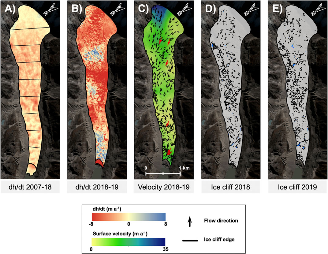
FIGURE 3. Spatial distribution of surface elevation change (dh/dt) for the (A) 2007–2018 and (B) 2018–2019 periods. (C) 2018–2019 surface flow velocity field. Ice cliff distributions (cliff edges highlighted) and supraglacial ponds in (D) October 2018 and (E) October 2019. The section boundaries are indicated in (A). Both the pre- and post-terminus positions are shown in (A) and (B). Red arrows in (C) are the stake-measured surface flow vectors.
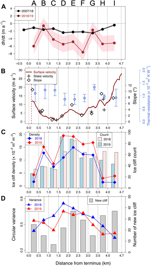
FIGURE 4. Section means of the (A) surface elevation change rate (dh/dt), (B) longitudinal surface flow velocity profile, stake displacement rate, thermal resistance (Fujita and Sakai, 2014), and section slopes in 2019, (C) ice cliff density and ice cliff count, and (D) circular variance of the ice cliff aspect and number of new ice cliffs in 2019. Glacier-wide segments A–I are 500-m-long segments that extend up-glacier from the terminus. The distance on the x-axis refers to the terminus position in October 2018 (0.0 km); the dashed line in (B) indicates the terminus position in 2019. The shaded region in (A) denotes the elevation change uncertainties (standard deviation of the SfM-DEMs pair; Table 2).
Uncertainty in Ice Cliff Delineation
We calculated the standard deviations of the edge length and map-view area of each ice cliff that was delineated by the five operators (Supplementary Figure S5), and employed the mean standard deviations (6.0 m for the cliff edge length and 24 m2 for map-view area of a cliff) as the delineation uncertainty. The corresponding uncertainties are estimated to be ±12.5% (2018) and ±11.4% (2019) for the edge length, and ±8.3% (2018) and ±6.9% (2019) for the map-view area, respectively. The cliff inclined area uncertainties that are associated with the map-view area uncertainties are ±8.1% (2018) and ±6.7% (2019). The additional uncertainty of the inclined area, which is associated with a slope angle uncertainty of ±1°, does not exceed ±2%.
Ice Cliff Characteristics
We extracted 481 and 505 ice cliffs from the 2018 and 2019 ortho-images, respectively (Figures 3D,E). The total ice cliff map-view areas were 138 × 103 m2 (4.7% of the study area) and 176 × 103 m2 (6.1%) in 2018 and 2019, respectively. The ice cliff length densities for the entire study area were 7.9 × 10⁻³ and 9.1 × 10⁻³ m m−2 in 2018 and 2019, respectively. The average ice cliff aspects were 335° (2018) and 325° (2019), which clearly suggested the predominance of northwest-facing ice cliffs (Figure 5A). We also calculated the morphological characteristics of the ice cliffs (Table 3). We found a strong positive correlation (r = 0.87, p < 0.001) between the ice cliff edge length and inclined area, with a power-law fit confirming the strong relationship between these ice cliff characteristics (R2 = 0.85, p < 0.001; Figure 5B). The power-law fit makes it possible to estimate the cliff inclined area from cliff edge length, which can be delineated from rather lower-resolution images. Supraglacial ponds covered 113 × 102 m2 (0.4% of the study area) in 2018 and 130 × 102 m2 (0.5%) in 2019. Approximately 83 and 74% of the total pond areas in 2018 and 2019, respectively, were adjacent to ice cliffs. Conversely, 15% (2018) and 8% (2019) of ice cliffs in the map-view area were adjacent to supraglacial ponds.
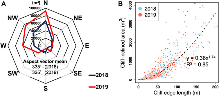
FIGURE 5. (A) Ice cliff aspect chart for the cliff inclined area (m2) and (B) the relationship between ice cliff edge length and inclined area. The dashed line in (B) is a power-law fit curve based on the ice cliff edge length and inclined area.

TABLE 3. Morphological characteristics of the analyzed ice cliffs. The maximum (Max.), minimum (Min.), and median (Med.) values are provided.
Spatial Distribution of Ice Cliffs
The ice cliff density and ice cliff count were analyzed across the nine sections (Figure 4C), with both the highest ice cliff density and ice cliff count observed across the middle section (Section E) during both years. The section means of the long-term elevation change (2007–2018) and ice cliff density in 2018 exhibit a strong negative correlation (r = −0.80, p < 0.05), whereas no correlation between the annual surface elevation change (2018–2019) and ice cliff density is observed. The ice cliff densities tend to decrease from the middle to both the terminus and up-glacier sections of the study area. High ice cliff counts were observed in the middle section (Section E) and up-glacier sections (sections H and I). The high ice cliff numbers and low ice cliff densities observed in the up-glacier sections (sections H and I) indicate that this area generally has smaller ice cliffs (Figure 4C).
The circular variance is high across the middle sections (sections D–F: >0.6) and low across the up-glacier and terminus sections (sections A, H, and I; Figure 4D). The ice cliff orientations show that north-facing ice cliffs (northeast and northwest) are predominant across all of the sections, whereas the aspect proportions vary among the sections (Figure 6). The south-facing ice cliffs (southwest and southeast) possess higher aspect proportions (>30%) across the middle sections (sections D–F) than across the terminus and up-glacier sections, which explains the large ice cliff variance across the middle sections (Figure 4D).
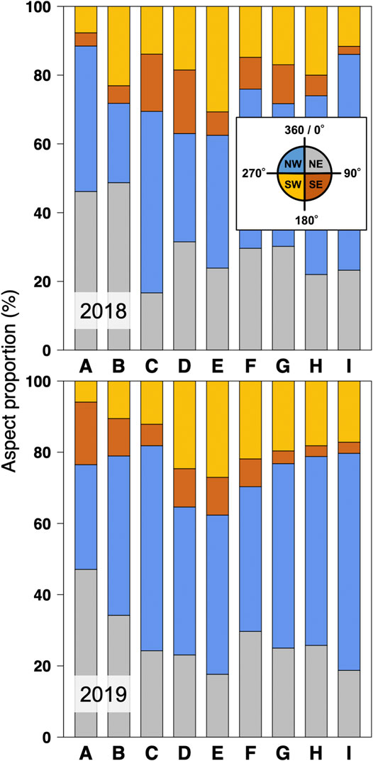
FIGURE 6. Count proportion of the ice cliff aspect across each section (A–I) in 2018 (upper) and 2019 (lower).
Temporal Changes in Ice Cliffs and Supraglacial Streams
Our ice cliff tracking analysis shows that 45% of the ice cliffs and 14% of their inclined area disappeared between 2018 and 2019 (Table 4). The ice cliff aspect is summarized for each ice cliff type in Figure 7. Most of the survived-2018 and -2019 ice cliffs are north-facing (∼80%; Figures 7B,C), with the disappeared and new ice cliffs consisting of more south-facing cliffs (∼35%) than the survived ice cliffs (∼20%; Figure 7). The circular variance for each ice cliff type also supports the aspect alignment of the survived ice cliffs and the aspect heterogeneity of the disappeared and new ice cliffs (Figure 7).

TABLE 4. Number and inclined area of each ice cliff type (disappeared, survived-2018, survived-2019, new, and non-classified). The corresponding percentages are shown in parentheses.
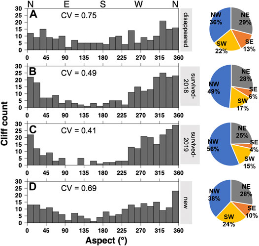
FIGURE 7. Histogram of each type of ice cliff aspect: (A) disappeared, (B) survived-2018, (C) survived-2019, and (D) new. CV is the circular variance of each type of ice cliff aspect. Pie charts show each ice cliff type’s aspect percentage (cliff count).
The ice cliff inclined area and slope also exhibit significant differences among the four ice cliff types (Table 5). The mean inclined area of the survived-2018 ice cliffs was significantly larger than that of the disappeared ice cliffs (p < 0.001 via Welch’s t-test), and the survived-2019 ice cliffs had a larger inclined area than the new ice cliffs (p < 0.001). Furthermore, the disappeared cliffs had gentler slopes than the survived-2018 ice cliffs (p < 0.05), and the survived-2019 ice cliffs had significantly steeper slopes than the new ice cliffs (p < 0.001). A comparison of the survived-2018 and -2019 ice cliff morphologies revealed that the survived-2018 ice cliffs became significantly larger (p < 0.05) and steeper (p < 0.001) over time (Table 5). The aspect dependency of the survived ice cliffs shows that the northwest-facing cliffs mostly expanded (170% increase in the inclined area) from 2018 to 2019 (Supplementary Table S3). We plotted the new ice cliffs and counted the number in each section (Figures 4D, 8A). More new ice cliffs formed across the middle (sections E and F), terminus (Section A), and up-glacier sections (sections H and I). Our supraglacial water flow analysis with the observed conduits is shown in Figure 8, which used nine exposed conduits that were identified from the aerial and terrestrial observations in 2019. The thermal resistance is relatively high in the terminus sections (sections A–C) and low in the middle to upper sections (sections D–I; Figure 4B).

TABLE 5. Mean inclined area and slope angle of each ice cliff type.
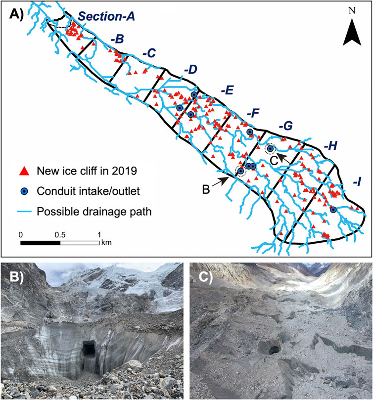
FIGURE 8. (A) Locations of the new ice cliffs, conduit intakes or outlets, and possible drainage paths in 2019. (B) and (C) Photographs of a conduit intake or outlet hole. The arrows on panel (A) show the directions from which the photographs were taken; the conduit holes in (B) and (C) are circled in (A). (B) is a terrestrial photograph, and (C) was acquired by UAV (Phantom 4) oblique movie.
Discussion
Ice Cliff Distribution and Morphology
The ice cliffs across Trakarding Glacier cover 4.7 and 6.1% of the debris-covered area, with ice cliff length densities of 7.9 and 9.1 × 10⁻³ m m−2 in 2018 and 2019, respectively. Our ice cliff coverage ratios are larger than the 0.2–3.9% values obtained for individual glaciers in the Langtang catchment (the maximum ratio was observed on Langtang Glacier, May 2015, Steiner et al., 2019), and our ice cliff length densities are higher than the highest ice cliff length density of 7.4 × 10⁻³ m−1 on Lhotse Shar Glacier, Khumbu region, in May 2009 (out of 14 glaciers, Watson et al., 2017a). Trakarding Glacier has a denser ice cliff distribution than other glaciers in the Nepal Himalaya, although we note that these previous analyses were conducted at coarser spatial resolutions. We also confirmed the remarkable spatial adjacency of supraglacial ponds to ice cliffs (83% of total pond area in 2018 and 74% in 2019) that has been reported in previous studies (Thompson et al., 2016; Watson et al., 2017a; Steiner et al., 2019), with our analysis obtaining a similar value to that reported by Watson et al. (2017a) for the Khumbu region (77% of the total pond area). It has been suggested that this spatial relationship generates thermal undercutting of the ice cliff, and further enhances cliff ablation (Kraaijenbrink P. D. A. et al., 2016; Miles et al., 2016; Watson et al., 2017b). In the present study, we conducted annual monitoring of the spatial distribution of supraglacial ponds and ice cliffs to investigate their spatial adjacency. However, Steiner et al. (2019) reported that seasonal variations can exist in areas occupied by ice cliffs and ponds. Therefore, a better understanding of the spatial relationship between ice cliffs and supraglacial ponds can be obtained by increasing the temporal resolution of the monitoring observations.
We find a strong correlation between the ice cliff edge length and inclined area (Figure 5B). Previous studies have delineated the ice cliff edge from high-resolution satellite imagery and DEMs (Thompson et al., 2016; Watson et al., 2017a). However, Steiner et al. (2019) mentioned the difficulty in estimating the inclined area of steep ice cliffs from satellite DEMs with meter-scale resolution. Combining aerial photogrammetry with the SfM method can generate super-high-resolution DEMs that enable the effective analysis of ice cliff slope morphology; however, we note that the UAV acquisition method has coverage and cost limitations. Our results suggest that the ice cliff inclined area can be inferred from the ice cliff edge length, which can be extracted from high-resolution satellite images when UAV-based DEMs are not available.
The ice cliff slope distribution peaked at 40°–45° (32% of all ice cliffs; Supplementary Figure S7; Kraaijenbrink P. D. A. et al. (2016)) analyzed the ice cliff slopes in the terminus area of Langtang Glacier using UAV-based DEMs, where they determined a mean slope of 45°, with 50% of the exposed ice cliff slopes in the 35°–42° range. Buri and Pellicciotti (2018) also reported that the mean ice cliff slope on Lirung Glacier was 40°, using a UAV-based DEM. These similar results suggest that ice cliff slopes are commonly in the 35°–45° range in the Nepal Himalaya. Sakai et al. (2002) reported that there were no ice cliffs with <30° slopes, and estimated the angle of repose for the debris mantle to be 30°–35° on Lirung Glacier. We find that ice cliffs with gentler slopes (<30°) comprised only 3.5% of the total ice cliff area. The median inclined area of these gently sloping ice cliffs (64 m2) was smaller than that of all the ice cliffs (162 m2). Furthermore, the disappeared ice cliffs had smaller inclined areas and gentler slopes than the survived-2018 ice cliffs (Table 5). These results suggest that most gently sloping ice cliffs are in the process of being buried by debris, which is in agreement with a previous study (Sakai et al., 2002), and are therefore disappearing.
Ice Cliff Orientation and Temporal Changes
The north-facing ice cliffs are more predominant than the south-facing ice cliffs across the studied debris-covered area (Figure 5A). Previous studies have hypothesized that the north-facing ice cliffs tended to persist, whereas the south-facing ice cliffs would often decay in the Nepal Himalaya since they receive direct shortwave radiation along their clifftops (e.g., Sakai et al., 2002; Buri and Pellicciotti, 2018). The different melting rates at the top and base of the ice cliffs lead to a gentler slope, such that the cliffs will eventually become debris-covered (Sakai et al., 1998). Conversely, the north-facing ice cliffs provide their own shade, such that ice cliff melting is controlled by longwave radiation from the warm debris mounds beside the ice cliffs (Sakai et al., 2002; Steiner et al., 2015; Buri et al., 2016). Therefore, the north-facing ice cliffs could retreat while preserving their steep slopes. The ablation season in High Mountain Asia coincides with the monsoon season, especially in the Himalayan region. Therefore, the glaciers are often shaded by cloud in the afternoon, such that they are protected from solar radiation from the southwest. Therefore, these glaciers suffer from stronger solar radiation from the southeast, with this energy flux leading to the survival of northwest-facing ice cliffs and the disappearance of southeast-facing ice cliffs (Sakai et al., 1998; Buri and Pellicciotti, 2018). The predominance of north-facing ice cliffs has also been observed in the Khumbu and Langtang regions via high-resolution satellite image analysis (Thompson et al., 2016; Watson et al., 2017a; Steiner et al., 2019). Our results are consistent with those presented in these previous studies, with the predominance of north-facing ice cliffs observed in remote-sensing data.
We find that the number of survived-2018 ice cliffs is higher than the number of disappeared ice cliffs (Table 4), whereas Steiner et al. (2019) reported that 50% of the ice cliffs survived between 2014 and 2015 across Langtang Glacier. However, the inclined areas of the new and disappeared ice cliffs are <15% of the total area in both 2018 and 2019 (Table 4). This result suggests the importance of estimating the melting of survived ice cliffs to determine the melting contribution of ice cliffs to glacier ablation. We also confirm a significant change in the survived ice cliffs, which became steeper and extended between 2018 and 2019 (Table 5). This suggests that the survived ice cliffs tend to evolve into more suitable forms for survival. Approximately 17% of the ice cliffs across Langtang Glacier, central Himalaya, survived during their decade-long study period (2006–2015, Steiner et al., 2019). It is therefore necessary to also conduct annual tracking of the ice cliffs for an extended period to better capture the survival of ice cliffs across Trakarding Glacier. We also note that the four ice cliff types possess different aspect proportions. The south-facing cliffs (southeast to southwest) are dominated by disappeared- and survived-2018 ice cliffs, with the disappeared ice cliffs possessing 12% higher south-facing aspect proportions than the survived-2018 ice cliffs (Figures 7A,B). This result also supports the survival hypothesis of north-facing ice cliffs. The new ice cliffs possess higher south-facing proportions and circular variances than the survived-2019 ice cliffs (Figure 7C, D). This is the first documented instance of observing and documenting the randomness of the new ice cliff aspects across a debris-covered glacier.
Ice Cliff Formation and Dynamics Across Trakarding Glacier
A large number of new ice cliffs are distributed across the up-glacier (sections H and I), middle (sections D–F), and terminus (Section A) sections of Trakarding Glacier (Figures 4D, 8A). The formation mechanisms of these ice cliffs may vary by section, owing to spatial differences in glacier dynamics and morphology. The up-glacier sections (sections H and I) are covered by a thin debris layer and possess a steeper slope (∼8°) than the other sections (Figure 4B). This condition would enhance ice melting, even at the higher elevations, which is evidenced by recent stake measurements (Sunako et al., 2019). Spatially heterogeneous melting rates increase the potential for the mass wasting of debris from the debris mound. The ice cliffs that form via this mechanism are likely to be small, as suggested by the coincidence of high cliff count and low cliff density in the up-glacier section (Figure 4C). Such small cliffs are unlikely to grow into large ice cliffs because they are easily buried by debris. A high cliff count, large number of new ice cliffs, and low ice cliff density are therefore observed across the up-glacier sections (sections H and I; Figures 4C,D).
The surface slope is gentle (∼2°) and the surface velocity decreases from the up-glacier to middle sections (sections F and G; Figure 4B). Previous studies have indicated that large supraglacial ponds tend to form under these topographic characteristics (e.g., Quincey et al., 2007; Sakai and Fujita, 2010; Salerno et al., 2012; Miles et al., 2017a). The up-glacier supply of meltwater pools is supraglacial ponds that form along the gentle slope and hummocky sections of sections F and G. These ponds could be heated by thermal exchange with the atmosphere, enhancing the potential for heated pond water to expand the englacial conduits when it flows through the englacial hydrological system (e.g., Benn et al., 2001; Röhl, 2008; Watson et al., 2016; Watson et al., 2018; Narama et al., 2017). Several exposed conduit holes have been observed across Section G, and are considered the intake points of englacial conduits (Figures 8A–C). The up-glacier supply of supraglacial water would pour into the englacial hydrological system along the middle sections (sections G and F; Figure 8A), even after these large supraglacial ponds have disappeared, further expanding the englacial conduits. Such a hydrological system with supraglacial water flow into englacial channels has also been observed along Ngozumpa (Benn et al., 2012; Benn et al., 2017) and Khumbu (Gulley et al., 2009; Miles et al., 2019) glaciers. A dense englacial conduit network is therefore inferred to exist along the gently sloping middle sections (sections F and G) of Trakarding Glacier.
A large number, high density, and high circular variance (randomness of aspect orientation) of the ice cliffs observed across the middle sections (sections D–F; Figures 4C,D, 6) are considered to have a strong relationship with supraglacial and englacial hydrological systems. Previous studies have suggested that ice cliffs can form via (1) the incision of supraglacial streams (e.g., Anderson et al., 2019b; Mölg et al., 2020) and/or (2) the collapse of englacial conduits on debris-covered glaciers (e.g., Sakai et al., 2000b; Gulley and Benn, 2007; Benn et al., 2012; Miles et al., 2017b). The spatial coincidence of the potential drainage pathways and newly formed ice cliffs are confirmed in the gentle upper-middle sections (sections F and G; Figure 8A). Such a spatial coincidence between supraglacial streams and ice cliffs has also been observed in Alaska (Anderson et al., 2019b) and the European Alps (Mölg et al., 2020). Supraglacial streams could be a potential source of new ice cliffs through incision and erosion of the flat glacier surface (Mölg et al., 2020). Supraglacial streams tend to meander across the glacier surface and undercut it, especially on gentle surface slopes, promoting the formation and persistence of ice cliffs (Anderson et al., 2019b). The middle sections are also likely to possess a dense englacial hydrological network, such that new ice cliffs may form via the collapse of these conduits (Supplementary Figure S8A). The collapse of a conduit leads to the formation of multiple new ice cliffs with random orientations, resulting in the observed high circular variance of the ice cliffs across the middle sections (Figures 4D, 6). These new ice cliffs are inferred to have aspect inhomogeneity, owing to their ice cliff formation mechanism (Temporal Changes in Ice Cliffs and Supraglacial Streams; Figure 7D). The newly formed ice cliffs would promote local ice ablation after the collapse of the englacial conduit, such that the up-glacier supply of meltwater may then form supraglacial ponds adjacent to the ice cliffs. Such a cliff-pond system creates a positive feedback for the expansion of the englacial hydrological system and new ice cliff formation. Therefore, a high ice cliff density, large number of new ice cliffs, and high aspect variance are observed along the middle sections (sections D–F), coincident with rapid surface lowering (Figures 4A,C,D). We identify a strong negative correlation between the ice cliff density and long-term surface elevation change (r = −0.80, p < 0.05), which suggests that the newly formed ice cliffs along the middle sections and conduit collapse have contributed to glacier thinning at the decadal scale (2007–2018). A similar relationship between the ice cliff distribution and surface lowering has been reported across the Langtang region (Ragettli et al., 2016) and the Khumbu region (Watson et al., 2017a).
The surface flow velocity decreases across the middle section (Section D; Figure 4B), suggesting the prevalence of longitudinal compression, which could promote closure of the englacial conduit network. Ice cliff formation owing to the collapse of englacial conduits would therefore decrease, resulting in lower ice cliff densities across Section D. Such a closure of the englacial conduit network in a compressive regime has been suggested in a previous study on Langtang Glacier (Kraaijenbrink P. D. A. et al., 2016). The surface flow velocity then increases again toward the terminal sections (sections A and B; Figures 4B,D), with the new ice cliffs in these sections likely forming as a result of crevassing (Supplementary Figure S8B). The low circular variances of these new cliffs are primarily north-facing, which is consistent with the glacier flow direction (Figures 4D, 6).
New ice cliffs have formed across the up-glacier, middle, and terminus sections of Trakarding Glacier; however, the ice cliff number and formation processes are different across each section. A large number of new and survived ice cliffs are distributed across the stagnant middle section, thereby contributing to the relatively large decadal-scale surface lowering across this section. We identify the spatial heterogeneity of the ice cliff aspect as a potential indicator of the ice cliff formation mechanism (e.g., conduit collapse or incision). However, we have not directly detected the ice cliff formation processes via an analysis of our high-resolution imagery over a one-year interval. Additional seasonal or monthly aerial photogrammetry surveying has the potential to identify the formation mechanism of individual ice cliffs. Previous studies have evaluated the contribution of ice cliff mass loss to glacier-scale mass balance (Brun et al., 2018; Anderson et al., 2019b). It is important to obtain such data sets to discuss the relationship between ice cliff dynamics and glacier mass balance, and quantify the mass loss contribution due to ice cliffs.
Conclusion
Here we presented the decadal and annual surface elevation changes and recent ice cliff dynamics across the debris-covered Trakarding Glacier, eastern Nepal Himalaya, using high-resolution aerial photogrammetry. We analyzed the remote-sensing data from three aerial photogrammetry surveys that were conducted during the 2007, 2018, and 2019 post-monsoon seasons, and generated DEMs via SfM. We also manually generated ice cliff inventories from the 2018 and 2019 SfM-DEMs and ortho-images. The morphology, spatial distribution, and temporal changes of the ice cliffs were analyzed using these high-resolution inventories. Ice cliffs covered 4.7 and 6.1% of the debris-covered area in 2018 and 2019, respectively. The ice cliff edge length correlates strongly with the ice cliff inclined area, which enables us to estimate the ice cliff inclined area from coarser satellite-based images when very-high-resolution DEMs are lacking. Our annual tracking of ice cliffs indicates that the disappeared ice cliff inclined area occupied 14% of the total ice cliff inclined area in 2018, with the newly formed ice cliff inclined area accounting for almost the same percentage in 2019. The new ice cliffs that formed in 2019 generally possessed a random aspect, smaller inclined area, and gentler slope than the survived ice cliffs. The survived ice cliffs generally have predominantly northwest-facing, steep slopes, and large inclined areas. The disappeared ice cliffs have a higher south-facing aspect count proportion than the survived ice cliffs. Our results support the hypothesis of persisting north-facing ice cliffs that has been suggested by previous studies. Greater circular variance is observed in the middle and terminus sections of the glacier, which indicates the formation of new ice cliffs with random aspects.
We could elucidate the factors potentially controlling ice cliff dynamics (e.g., glacier flow velocity field, off glacier terrain, and meteorological conditions) by applying the ice cliff classification demonstrated in this study to glaciers in other regions. Although we only focused on the surface elevation changes in this study, it is important to quantify the mass loss contribution of ice cliffs to the total glacier mass balance. Ice thickness and flow velocity distributions are required to estimate the emergence velocity, which is an upward motion of the ice that compensates the glacier ablation. Evaluating both the dynamics and mass loss of ice cliffs will allow us to elucidate the quantitative impact of ice cliffs on the ablation of debris-covered glaciers.
Data Availability Statement
The raw data supporting the conclusions of this article will be made available by the authors, without undue reservation.
Author Contributions
KF designed the study. YS, KF, SS, HI, AT, AS, EP, and RK conducted the field observations with the support of RK, YS processed the photogrammetry data, and SS and KF analyzed the GPS data. YS, KF, AS, and EP wrote the manuscript. All of the authors contributed to the discussion.
Funding
This study was supported by JSPS-KAKENHI (grant numbers 17H01621 and 18KK0098), and JSPS and SNSF under the Joint Research Projects (JRPs; grant number 20191503).
Conflict of Interest
The authors declare that the research was conducted in the absence of any commercial or financial relationships that could be construed as a potential conflict of interest.
Acknowledgments
We thank Etienne Berthier for providing the Pléiades satellite data. We are indebted to Guide For All Seasons Trek for logistical support during the fieldwork. The Asahi Shimbun Company supported the aerial photogrammetry survey in 2007. We acknowledge three reviewers for their constructive and insightful comments.
Supplementary Material
The Supplementary Material for this article can be found online at: https://www.frontiersin.org/articles/10.3389/feart.2021.623623/full#supplementary-material
References
Agisoft LLC (2020). Agisoft Metashape User Manual Professional Edition, Version 1.6. Available at: https://www.agisoft.com/pdf/metashape-pro_1_6_en.pdf. (Accessed April 1, 2020)
Anderson, L. S., Armstrong, W. H., Anderson, R. S., and Buri, P. (2019a). Debris Cover and the Thinning of Kennicott Glacier, Alaska, Part B: Ice Cliff Delineation and Distributed Melt Estimates. Cryosphere Discuss. doi:10.5194/tc-2019-177
Anderson, L. S., Armstrong, W. H., Anderson, R. S., and Buri, P. (2019b). Debris Cover and the Thinning of Kennicott Glacier, Alaska, Part C: Feedbacks between Melt, Ice Dynamics, and Surface Processes. Cryosphere Discuss. doi:10.5194/tc-2019-178
Benn, D. I., Wiseman, S., and Hands, K. A. (2001). Growth and Drainage of Supraglacial Lakes on Debris-Mantled Ngozumpa Glacier, Khumbu Himal, Nepal. J. Glaciol. 47, 626–638. doi:10.3189/172756501781831729
Benn, D. I., Bolch, T., Hands, K., Gulley, J., Luckman, A., Nicholson, L. I., et al. (2012). Response of Debris-Covered Glaciers in the Mount Everest Region to Recent Warming, and Implications for Outburst Flood Hazards. Earth-Science Rev. 114, 156–174. doi:10.1016/j.earscirev10.1016/j.earscirev.2012.03.008
Benn, D. I., Thompson, S., Gulley, J., Mertes, J., Luckman, A., and Nicholson, L. (2017). Structure and Evolution of the Drainage System of a Himalayan Debris-Covered Glacier, and its Relationship with Patterns of Mass Loss. The Cryosphere 11, 2247–2264. doi:10.5194/tc-11-2247-2017
Berthier, E., Arnaud, Y., Kumar, R., Ahmad, S., Wagnon, P., and Chevallier, P. (2007). Remote Sensing Estimates of Glacier Mass Balances in the Himachal Pradesh (Western Himalaya, India). Remote Sensing Environ. 108, 327–338. doi:10.1016/j.rse.2006.11.017
Berthier, E., Vincent, C., Magnússon, E., Gunnlaugsson, Á. Þ., Pitte, P., Le Meur, E., et al. (2014). Glacier Topography and Elevation Changes Derived from Pléiades Sub-meter Stereo Images. The Cryosphere 8, 2275–2291. doi:10.5194/tc-8-2275-2014
Bolch, T., Kulkarni, A., Kääb, A., Huggel, C., Paul, F., Cogley, J. G., et al. (2012). The State and Fate of Himalayan Glaciers. Science 336, 310–314. doi:10.1126/science.1215828
Brun, F., Berthier, E., Wagnon, P., Kääb, A., and Treichler, D. (2017). A Spatially Resolved Estimate of High Mountain Asia Glacier Mass Balances from 2000 to 2016. Nat. Geosci 10, 668–673. doi:10.1038/NGEO2999
Brun, F., Wagnon, P., Berthier, E., Shea, J. M., Immerzeel, W. W., Kraaijenbrink, P. D. A., et al. (2018). Ice Cliff Contribution to the Tongue-wide Ablation of Changri Nup Glacier, Nepal, Central Himalaya. The Cryosphere 12, 3439–3457. doi:10.5194/tc-12-3439-2018
Brun, F., Wagnon, P., Berthier, E., Jomelli, V., Maharjan, S. B., Shrestha, F., et al. (2019). Heterogeneous Influence of Glacier Morphology on the Mass Balance Variability in High Mountain Asia. J. Geophys. Res. Earth Surf. 124, 1331–1345. doi:10.1029/2018JF004838
Buri, P., and Pellicciotti, F. (2018). Aspect Controls the Survival of Ice Cliffs on Debris-Covered Glaciers. Proc. Natl. Acad. Sci. USA 115, 4369–4374. doi:10.1073/pnas.1713892115
Buri, P., Miles, E. S., Steiner, J. F., Immerzeel, W. W., Wagnon, P., and Pellicciotti, F. (2016). A Physically Based 3‐D Model of Ice Cliff Evolution over Debris‐covered Glaciers. J. Geophys. Res. Earth Surf. 121, 2471–2493. doi:10.1002/2016JF004039
Fujita, K., and Sakai, A. (2014). Modelling Runoff from a Himalayan Debris-Covered Glacier. Hydrol. Earth Syst. Sci. 18, 2679–2694. doi:10.5194/hess-18-2679-2014
Fujita, K., Suzuki, R., Nuimura, T., and Sakai, A. (2008). Performance of ASTER and SRTM DEMs, and Their Potential for Assessing Glacial Lakes in the Lunana Region, Bhutan Himalaya. J. Glaciol. 54, 220–228. doi:10.3189/002214308784886162
Fujita, K., Sakai, A., Takenaka, S., Nuimura, T., Surazakov, A. B., Sawagaki, T., et al. (2013). Potential Flood Volume of Himalayan Glacial Lakes. Nat. Hazards Earth Syst. Sci. 13, 1827–1839. doi:10.5194/nhess-13-1827-2013
Fujita, K., Inoue, H., Izumi, T., Yamaguchi, S., Sadakane, A., Sunako, S., et al. (2017). Anomalous Winter-Snow-Amplified Earthquake-Induced Disaster of the 2015 Langtang Avalanche in Nepal. Nat. Hazards Earth Syst. Sci. 17, 749–764. doi:10.5194/nhess-17-749-2017
Gardelle, J., Berthier, E., Arnaud, Y., and Kääb, A. (2013). Region-wide Glacier Mass Balances over the Pamir-Karakoram-Himalaya during 1999-2011. The Cryosphere 7, 1263–1286. doi:10.5194/tc-7-1263-2013
Gulley, J., and Benn, D. I. (2007). Structural Control of Englacial Drainage Systems in Himalayan Debris-Covered Glaciers. J. Glaciol. 53, 399–412. doi:10.3189/002214307783258378
Gulley, J. D., Benn, D. I., Screaton, E., and Martin, J. (2009). Mechanisms of Englacial Conduit Formation and Their Implications for Subglacial Recharge. Quat. Sci. Rev. 28, 1984–1999. doi:10.1016/j.quascirev.2009.04.002
Han, H., Wang, J., Wei, J., and Liu, S. (2010). Backwasting Rate on Debris-Covered Koxkar Glacier, Tuomuer Mountain, China. J. Glaciol. 56, 287–296. doi:10.3189/002214310791968430
Herreid, S., and Pellicciotti, F. (2020). The State of Rock Debris Covering Earth's Glaciers. Nat. Geosci. 13, 621–627. doi:10.1038/s41561-020-0615-0
Immerzeel, W. W., Kraaijenbrink, P. D. A., Shea, J. M., Shrestha, A. B., Pellicciotti, F., Bierkens, M. F. P., et al. (2014). High-resolution Monitoring of Himalayan Glacier Dynamics Using Unmanned Aerial Vehicles. Remote Sensing Environ. 150, 93–103. doi:10.1016/j.rse.2014.04.025
Kääb, A., Berthier, E., Nuth, C., Gardelle, J., and Arnaud, Y. (2012). Contrasting Patterns of Early Twenty-First-Century Glacier Mass Change in the Himalayas. Nature 488, 495–498. doi:10.1038/nature11324
Kraaijenbrink, P., Meijer, S. W., Shea, J. M., Pellicciotti, F., De Jong, S. M., and Immerzeel, W. W. (2016). Seasonal Surface Velocities of a Himalayan Glacier Derived by Automated Correlation of Unmanned Aerial Vehicle Imagery. Ann. Glaciol. 57, 103–113. doi:10.3189/2016AoG71A072
Kraaijenbrink, P. D. A., Shea, J. M., Pellicciotti, F., Jong, S. M. d., and Immerzeel, W. W. (2016). Object-based Analysis of Unmanned Aerial Vehicle Imagery to Map and Characterise Surface Features on a Debris-Covered Glacier. Remote Sensing Environ. 186, 581–595. doi:10.1016/j.rse.2016.09.013
Lamsal, D., Fujita, K., and Sakai, A. (2017). Surface Lowering of the Debris-Covered Area of Kanchenjunga Glacier in the Eastern Nepal Himalaya since 1975, as Revealed by Hexagon KH-9 and ALOS Satellite Observations. The Cryosphere 11, 2815–2827. doi:10.5194/tc-11-2815-2017
Lucieer, A., Jong, S. M. d., and Turner, D. (2014). Mapping Landslide Displacements Using Structure from Motion (SfM) and Image Correlation of Multi-Temporal UAV Photography. Prog. Phys. Geogr. Earth Environ. 38, 97–116. doi:10.1177/0309133313515293
Mattson, L. E., Gardner, J. S., and Young, G. J. (1993). Ablation on Debris Covered Glaciers: an Example from the Rakhiot Glacier, Punjab, Himalaya. IAHS Publ. 218 (Symposium at Seattle 2000 – Debris-Covered Glaciers), 289–296.
Miles, E. S., Pellicciotti, F., Willis, I. C., Steiner, J. F., Buri, P., and Arnold, N. S. (2016). Refined Energy-Balance Modelling of a Supraglacial Pond, Langtang Khola, Nepal. Ann. Glaciol. 57, 29–40. doi:10.3189/2016AoG71A421
Miles, E. S., Willis, I. C., Arnold, N. S., Steiner, J., and Pellicciotti, F. (2017a). Spatial, Seasonal and Interannual Variability of Supraglacial Ponds in the Langtang Valley of Nepal, 1999-2013. J. Glaciol. 63, 88–105. doi:10.1017/jog.2016.120
Miles, E. S., Steiner, J., Willis, I., Buri, P., Immerzeel, W. W., Chesnokova, A., et al. (2017b). Pond Dynamics and Supraglacial-Englacial Connectivity on Debris-Covered Lirung Glacier, Nepal. Front. Earth Sci. 5, 69. doi:10.3389/feart.2017.00069
Miles, K. E., Hubbard, B., Quincey, D. J., Miles, E. S., Irvine-Fynn, T. D. L., and Rowan, A. V. (2019). Surface and Subsurface Hydrology of Debris-Covered Khumbu Glacier, Nepal, Revealed by Dye Tracing. Earth Planet. Sci. Lett. 513, 176–186. doi:10.1016/j.epsl.2019.02.020
Mölg, N., Ferguson, J., Bolch, T., and Vieli, A. (2020). On the Influence of Debris Cover on Glacier Morphology: How High-Relief Structures Evolve from Smooth Surfaces. Geomorphology 357, 107092. doi:10.1016/j.geomorph.2020.107092
Nakawo, M., and Young, G. J. (1982). Estimate of Glacier Ablation under a Debris Layer from Surface Temperature and Meteorological Variables. J. Glaciol. 28, 29–34. doi:10.3189/S002214300001176X
Narama, C., Daiyrov, M., Tadono, T., Yamamoto, M., Kääb, A., Morita, R., et al. (2017). Seasonal Drainage of Supraglacial Lakes on Debris-Covered Glaciers in the Tien Shan Mountains, Central Asia. Geomorphol. 286, 133–142. doi:10.1016/j.geomorph.2017.03.002
Nicholson, L., and Benn, D. I. (2006). Calculating Ice Melt beneath a Debris Layer Using Meteorological Data. J. Glaciol. 52, 463–470. doi:10.3189/172756506781828584
Nuimura, T., Fujita, K., Yamaguchi, S., and Sharma, R. R. (2012). Elevation Changes of Glaciers Revealed by Multitemporal Digital Elevation Models Calibrated by GPS Survey in the Khumbu Region, Nepal Himalaya, 1992-2008. J. Glaciol. 58, 648–656. doi:10.3189/2012JoG11J061
Nuimura, T., Sakai, A., Taniguchi, K., Nagai, H., Lamsal, D., Tsutaki, S., et al. (2015). The GAMDAM Glacier Inventory: a Quality-Controlled Inventory of Asian Glaciers. The Cryosphere 9, 849–864. doi:10.5194/tc-9-849-2015
O’Callaghan, J. F., and Mark, D. M. (1984). The Extraction of Drainage Networks from Digital Elevation Data. Comput. Vis. Graph. Image Process. 28, 323–344. doi:10.1016/S0734-189X(84)80011-0
Østrem, G. (1959). Ice Melting under a Thin Layer of Moraine, and the Existence of Ice Cores in Moraine Ridges. Geografiska Annaler 41, 228–230. doi:10.1080/20014422.1959.11907953
Pellicciotti, F., Stephan, C., Miles, E., Herreid, S., Immerzeel, W. W., and Bolch, T. (2015). Mass-balance Changes of the Debris-Covered Glaciers in the Langtang Himal, Nepal, from 1974 to 1999. J. Glaciol. 61, 373–386. doi:10.3189/2015JoG13J237
Podolskiy, E. A., Fujita, K., Sunako, S., Tsushima, A., and Kayastha, R. B. (2018). Nocturnal Thermal Fracturing of a Himalayan Debris-Covered Glacier Revealed by Ambient Seismic Noise. Geophys. Res. Lett. 45, 9699–9709. doi:10.1029/2018GL079653
Podolskiy, E. A., Fujita, K., Sunako, S., and Sato, Y. (2019). Viscoelastic Modeling of Nocturnal Thermal Fracturing in a Himalayan Debris‐Covered Glacier. J. Geophys. Res. Earth Surf. 124, 1485–1515. doi:10.1029/2018JF004848
Quincey, D. J., Richardson, S. D., Luckman, A., Lucas, R. M., Reynolds, J. M., Hambrey, M. J., et al. (2007). Early Recognition of Glacial Lake Hazards in the Himalaya Using Remote Sensing Datasets. Glob. Planet. Change 56, 137–152. doi:10.1016/j.gloplacha.2006.07.013
Ragettli, S., Bolch, T., and Pellicciotti, F. (2016). Heterogeneous Glacier Thinning Patterns over the Last 40 Years in Langtang Himal, Nepal. The Cryosphere 10, 2075–2097. doi:10.5194/tc-10-2075-2016
Röhl, K. (2008). Characteristics and Evolution of Supraglacial Ponds on Debris-Covered Tasman Glacier, New Zealand. J. Glaciol. 54, 867–880. doi:10.3189/002214308787779861
Sakai, A., and Fujita, K. (2010). Formation Conditions of Supraglacial Lakes on Debris-Covered Glaciers in the Himalaya. J. Glaciol. 56, 177–181. doi:10.3189/002214310791190785
Sakai, A., Nakawo, M., and Fujita, K. (1998). Melt Rate of Ice Cliffs on the Lirung Glacier, Nepal Himalayas, 1996. Bull. Glacier Res. 16, 57–66.
Sakai, A., Chikita, K., and Yamada, T. (2000a). Expansion of a Moraine-Dammed Glacial Lake, Tsho Rolpa, in Rolwaling Himal, Nepal Himalaya. Limnol. Oceanogr 45 (6), 1401–1408. doi:10.4319/lo.2000.45.6.1401
Sakai, A., Takeuchi, N., Fujita, K., and Nakawo, M. (2000b). Role of Supraglacial Ponds in the Ablation Process of a Debris-Covered Glacier in the Nepal Himalayas.IAHS Publ., no. 264.
Sakai, A., Nakawo, M., and Fujita, K. (2002). Distribution Characteristics and Energy Balance of Ice Cliffs on Debris-Covered Glaciers, Nepal Himalaya. Arctic, Antarctic, Alpine Res. 34, 12–19. doi:10.2307/1552503
Sakai, A. (2019). Brief Communication: Updated GAMDAM Glacier Inventory over High-Mountain Asia. The Cryosphere 13, 2043–2049. doi:10.5194/tc-13-2043-2019
Salerno, F., Thakuri, S., D’Agata, C., Smiraglia, C., Manfredi, E. C., Viviano, G., et al. (2012). Glacial Lake Distribution in the Mount Everest Region: Uncertainty of Measurement and Conditions of Formation. Glob. Planet. Change 92-93, 30–39. doi:10.1016/j.gloplacha.2012.04.001
Salerno, F., Thakuri, S., Tartari, G., Nuimura, T., Sunako, S., Sakai, A., et al. (2017). Debris-covered Glacier Anomaly? Morphological Factors Controlling Changes in the Mass Balance, Surface Area, Terminus Position, and Snow Line Altitude of Himalayan Glaciers. Earth Planet. Sci. Lett. 471, 19–31. doi:10.1016/j.epsl.2017.04.039
Shean, D. E., Bhushan, S., Montesano, P., Rounce, D. R., Arendt, A., and Osmanoglu, B. (2020). A Systematic, Regional Assessment of High Mountain Asia Glacier Mass Balance. Front. Earth Sci. 7, 363. doi:10.3389/feart.2019.00363
Steiner, J. F., Pellicciotti, F., Buri, P., Miles, E. S., Immerzeel, W. W., and Reid, T. D. (2015). Modelling Ice-Cliff Backwasting on a Debris-Covered Glacier in the Nepalese Himalaya. J. Glaciol. 61, 889–907. doi:10.3189/2015JoG14J194
Steiner, J. F., Buri, P., Miles, E. S., Ragettli, S., and Pellicciotti, F. (2019). Supraglacial Ice Cliffs and Ponds on Debris-Covered Glaciers: Spatio-Temporal Distribution and Characteristics. J. Glaciol. 65, 617–632. doi:10.1017/jog.2019.40
Sunako, S., Fujita, K., Sakai, A., and Kayastha, R. B. (2019). Mass Balance of Trambau Glacier, Rolwaling Region, Nepal Himalaya: In-Situ Observations, Long-Term Reconstruction and Mass-Balance Sensitivity. J. Glaciol. 65, 605–616. doi:10.1017/jog.2019.37
Thompson, S., Benn, D. I., Mertes, J., and Luckman, A. (2016). Stagnation and Mass Loss on a Himalayan Debris-Covered Glacier: Processes, Patterns and Rates. J. Glaciol. 62, 467–485. doi:10.1017/jog.2016.37
Tshering, P., and Fujita, K. (2016). First In Situ Record of Decadal Glacier Mass Balance (2003-2014) from the Bhutan Himalaya. Ann. Glaciol. 57, 289–294. doi:10.3189/2016AoG71A036
Vincent, C., Wagnon, P., Shea, J. M., Immerzeel, W. W., Kraaijenbrink, P., Shrestha, D., et al. (2016). Reduced Melt on Debris-Covered Glaciers: Investigations from Changri Nup Glacier, Nepal. The Cryosphere 10, 1845–1858. doi:10.5194/tc-10-1845-2016
Watson, C. S., Quincey, D. J., Carrivick, J. L., and Smith, M. W. (2016). The Dynamics of Supraglacial Ponds in the Everest Region, Central Himalaya. Glob. Planet. Change 142, 14–27. doi:10.1016/j.gloplacha.2016.04.008
Watson, C. S., Quincey, D. J., Carrivick, J. L., and Smith, M. W. (2017a). Ice Cliff Dynamics in the Everest Region of the Central Himalaya. Geomorphology 278, 238–251. doi:10.1016/j.geomorph.2016.11.017
Watson, C. S., Quincey, D. J., Smith, M. W., Carrivick, J. L., Rowan, A. V., and James, M. R. (2017b). Quantifying Ice Cliff Evolution with Multi-Temporal Point Clouds on the Debris-Covered Khumbu Glacier, Nepal. J. Glaciol. 63, 823–837. doi:10.1017/jog.2017.47
Watson, C. S., Quincey, D. J., Carrivick, J. L., Smith, M. W., Rowan, A. V., and Richardson, R. (2018). Heterogeneous Water Storage and Thermal Regime of Supraglacial Ponds on Debris-Covered Glaciers. Earth Surf. Process. Landforms 43, 229–241. doi:10.1002/esp.4236
Wigmore, O., and Mark, B. (2017). Monitoring Tropical Debris-Covered Glacier Dynamics from High-Resolution Unmanned Aerial Vehicle Photogrammetry, Cordillera Blanca, Peru. The Cryosphere 11, 2463–2480. doi:10.5194/tc-11-2463-2017
Keywords: ice cliff, high mountain asia, debris-covered glacier, unmanned aerial vehicles, Himalaya
Citation: Sato Y, Fujita K, Inoue H, Sunako S, Sakai A, Tsushima A, Podolskiy EA, Kayastha R and Kayastha RB (2021) Ice Cliff Dynamics of Debris-Covered Trakarding Glacier in the Rolwaling Region, Nepal Himalaya. Front. Earth Sci. 9:623623. doi: 10.3389/feart.2021.623623
Received: 30 October 2020; Accepted: 05 May 2021;
Published: 04 June 2021.
Edited by:
Timothy C. Bartholomaus, University of Idaho, United StatesReviewed by:
Leif S. Anderson, University of Lausanne, SwitzerlandQiao Liu, Chinese Academy of Sciences (CAS), China
Eric Petersen, University of Alaska Fairbanks, United States
Copyright © 2021 Sato, Fujita, Inoue, Sunako, Sakai, Tsushima, Podolskiy, Kayastha and Kayastha. This is an open-access article distributed under the terms of the Creative Commons Attribution License (CC BY). The use, distribution or reproduction in other forums is permitted, provided the original author(s) and the copyright owner(s) are credited and that the original publication in this journal is cited, in accordance with accepted academic practice. No use, distribution or reproduction is permitted which does not comply with these terms.
*Correspondence: Yota Sato, eW90YS5zYXRvQG5hZ295YS11Lmpw
†Present address: Akane Tsushima, Graduate School of Sciences, Chiba University, Chiba, Japan