3D Linked Subduction, Dynamic Rupture, Tsunami, and Inundation Modeling: Dynamic Effects of Supershear and Tsunami Earthquakes, Hypocenter Location, and Shallow Fault Slip

Physics-based dynamic rupture models capture the variability of earthquake slip in space and time and can account for the structural complexity inherent to subduction zones. Here we link tsunami generation, propagation, and coastal inundation with 3D earthquake dynamic rupture (DR) models initialized using a 2D seismo-thermo-mechanical geodynamic (SC) model simulating both subduction dynamics and seismic cycles. We analyze a total of 15 subduction-initialized 3D dynamic rupture-tsunami scenarios in which the tsunami source arises from the time-dependent co-seismic seafloor displacements with flat bathymetry and inundation on a linearly sloping beach. We first vary the location of the hypocenter to generate 12 distinct unilateral and bilateral propagating earthquake scenarios. Large-scale fault topography leads to localized up- or downdip propagating supershear rupture depending on hypocentral depth. Albeit dynamic earthquakes differ (rupture speed, peak slip-rate, fault slip, bimaterial effects), the effects of hypocentral depth (25–40 km) on tsunami dynamics are negligible. Lateral hypocenter variations lead to small effects such as delayed wave arrival of up to 100 s and differences in tsunami amplitude of up to 0.4 m at the coast. We next analyse inundation on a coastline with complex topo-bathymetry which increases tsunami wave amplitudes up to ≈1.5 m compared to a linearly sloping beach. Motivated by structural heterogeneity in subduction zones, we analyse a scenario with increased Poisson's ratio of ν = 0.3 which results in close to double the amount of shallow fault slip, ≈1.5 m higher vertical seafloor displacement, and a difference of up to ≈1.5 m in coastal tsunami amplitudes. Lastly, we model a dynamic rupture “tsunami earthquake” with low rupture velocity and low peak slip rates but twice as high tsunami potential energy. We triple fracture energy which again doubles the amount of shallow fault slip, but also causes a 2 m higher vertical seafloor uplift and the highest coastal tsunami amplitude (≈7.5 m) and inundation area compared to all other scenarios. Our mechanically consistent analysis for a generic megathrust setting can provide building blocks toward using physics-based dynamic rupture modeling in Probabilistic Tsunami Hazard Analysis.

1. Introduction

Earthquake sources are governed by highly non-linear multi-physics and multi-scale processes leading to large variability in dynamic and kinematic properties such as rupture speed, slip rate, energy radiation, and slip distribution (e.g., Oglesby et al., 2000; Kaneko et al., 2008; Gabriel et al., 2012; Bao et al., 2019; Ulrich et al., 2019a; Gabriel et al., 2020). Such variability may impact the generation, propagation, and inundation of earthquake-generated tsunami or secondary tsunami generation mechanisms such as triggered landslides (e.g., Sepúlveda et al., 2020). For example, unexpectedly large slip at shallow depths may generate large tsunami (Lay et al., 2011; Romano et al., 2014; Lorito et al., 2016).

To model earthquake-generated tsunami, sources can be approximated from earthquake generated uplift (Behrens and Dias, 2015, and references therein). Analytical solutions (e.g., Okada, 1985) describe seafloor displacements sourced by uniform rectangular dislocations within a homogeneous elastic half space. Models of tsunami generated by large earthquakes can routinely and quickly use kinematic finite fault models constrained by inversion of seismic, geodetic, and other geophysical data (Geist and Yoshioka, 1996; Ji et al., 2002; Babeyko et al., 2010; Maeda et al., 2013; Allgeyer and Cummins, 2014; Mai and Thingbaijam, 2014; Bletery et al., 2016; Jamelot et al., 2019), but are challenged by the inherent non-uniqueness of kinematic source models (Mai et al., 2016).

Probabilistic Tsunami Hazard Analysis (PTHA) requires the computation of thousands or millions of tsunami scenarios for each specific area of interest (González et al., 2009; Geist and Oglesby, 2014; Horspool et al., 2014; Geist and Lynett, 2014; Lorito et al., 2015; Selva et al., 2016; Grezio et al., 2017; Mori et al., 2018; Sepúlveda et al., 2019; Glimsdal et al., 2019). Stochastic source models (McCloskey et al., 2008; Davies and Griffin, 2019) statistically vary slip distributions (Andrews, 1980) and are specifically suited for PTHA in combination with efficient tsunami solvers (e.g., Berger et al., 2011; Nakano et al., 2020). For instance, Goda et al. (2014) highlights strong sensitivities of tsunami height to slip distribution and variations in fault geometry in stochastic random-field slip models for the 2011 Tohoku-Oki earthquake and tsunami. Recently, Scala et al. (2019) use stochastic slip distributions for PTHA in the Mediterranean area.

3D Dynamic earthquake rupture modeling can provide mechanically viable tsunami source descriptions on complex faults or fault systems on the scale of megathrust events (Galvez et al., 2014; Murphy et al., 2016; Uphoff et al., 2017; Murphy et al., 2018; Ma and Nie, 2019; Saito et al., 2019; Ulrich et al., 2020). Such simulations can exploit modern numerical methods and high-performance computing (HPC) to shed light on the dynamics and severity of earthquake behavior and potentially complement PTHA. For example, in dynamic rupture models shallow slip amplification can spontaneously emerge due to up-dip rupture facilitated by along-depth bi-material effects (Rubin and Ampuero, 2007; Ma and Beroza, 2008; Scala et al., 2017) and free-surface reflected waves within the accretionary wedge (Nielsen, 1998; Lotto et al., 2017a; van Zelst et al., 2019). Dynamic rupture earthquake models can yield stochastic slip distributions, too, under the assumption of stochastic loading stresses (Geist and Oglesby, 2014). Such physics-based models can be directly linked to tsunami models by using the time-independent or time-dependent seafloor displacements (and potentially velocities) as the tsunami source (Kozdon and Dunham, 2013; Ryan et al., 2015; Lotto et al., 2017b; Saito et al., 2019; Madden et al., 2020). For instance, time-dependent 3D displacements from observational constrained dynamic rupture scenarios of the 2018 Palu, Sulawesi earthquake and the 2004 Sumatra-Andaman earthquake are linked to a hydrostatic shallow water tsunami model by Ulrich et al. (2019b). Bathymetry induced amplification of horizontal displacements are thereby accounted for by following Tanioka and Satake (1996).

Observational and numerical studies show that megathrust geometry and hypocenter location influence earthquake rupture characteristics. Ye et al. (2016) state that megathrust earthquakes across faults that are longer horizontally than they are deep vertically (with an aspect ratio of three or larger) tend to exhibit primarily unilateral behavior. Also, events with an asymmetric hypocenter location on the fault favor rupture propagation along strike to its far end (Harris et al., 1991; McGuire et al., 2002; Hirano, 2019). Weng and Ampuero (2019) show the energetics of elongated ruptures is radically different from that of conventional circular crack models. Bilek and Lay (2018) find that the complexity of slip as well as bi- or unilateral rupture preferences of large earthquakes highly depend on the depth location of the hypocenter.

Subduction zones worldwide are associated with tectonic, frictional, and structural heterogeneity along depth and along-arc impacting megathrust earthquake and tsunami dynamics (Kirkpatrick et al., 2020, e.g.,). Kanamori and Brodsky (2004) show that fracture energy varies between subduction zone earthquakes. A special case are so called tsunami earthquakes (Kanamori, 1972) that may require a large amount of fracture energy, low rupture velocity and low radiation efficiency. Structural heterogeneity in subduction zones includes variations in Poisson's ratio (V_p/V_s) (e.g., Liu and Zhao, 2014; Niu et al., 2020)), while dynamic rupture and seismic wave propagation models often adopt an idealized Poisson's ratio of ν=0.25 governing seismic wave propagation (e.g., Kozdon and Dunham, 2013).

The initial conditions of dynamic rupture simulations that control earthquake rupture nucleation, propagation, and arrest include fault loading stresses, frictional strength, fault geometry, and subsurface material properties (e.g., Kame et al., 2003; Gabriel et al., 2013; Galis et al., 2015; Bai and Ampuero, 2017). These initial conditions may be observationally and empirically informed (e.g., Aochi and Fukuyama, 2002; Aagaard et al., 2004; Murphy et al., 2018; Ulrich et al., 2020) but remain difficult to constrain. Particularly in subduction zones where observational data are sparse, space and time scales vary over many orders of magnitude and both geometric and rheological megathrust complexities are likely to control rupture characteristics. Recently, initial conditions for 2D and 3D megathrust dynamic rupture earthquake models have been informed from 2D geodynamic long-term subduction and seismic cycle models (van Zelst et al., 2019; Madden et al., 2020; van Zelst et al., 2021). This approach provides self-consistent initial fault loading stresses and frictional strength, fault geometry and material properties on and surrounding the megathrust, as well as consistency with crustal, lithospheric, and mantle deformation and deformation in the subduction channel over geological time scales. Such subduction-initialized heterogeneous dynamic rupture models lead to complex earthquakes with multiple rupture styles (Gabriel et al., 2012), shallow slip accumulation and fault reactivation.

We apply the 2D geodynamical subduction and seismic cycle (SC) model from van Zelst et al. (2019) to inform realistic 3D dynamic rupture (DR) megathrust earthquake models within a complex, self-consistent subduction setup along with their consequent tsunami, following the subduction to tsunami run-up linking approach described in Madden et al. (2020). In this study we introduce a number of important differences to previous work. 2D linking including approximations to match SC and DR fracture energy during slip events leads to differences in slip magnitude between the SC and DR modeling and large magnitudes and high rupture speed in dynamic rupture scenarios (van Zelst et al., 2019). In contrast, we here constrain fracture energy independently from the long-term model. In Madden et al. (2020), a different long-term geodynamic and seismic cycle simulation was used, specifically, assuming different shear moduli. We here change the geometrical 3D extrapolation of the 2D fault geometry compared to the large blind dynamic earthquake scenario of M_W9.0 of Madden et al. (2020), to be consistent with empirical earthquake source scaling relations for M_W8.5 megathrust events (Strasser et al., 2010).

We use complex 3D dynamic rupture modeling to first study trade-offs and effects of along-strike unilateral vs. bilateral rupture and variations in hypocentral depth in subduction zone earthquakes (McGuire et al., 2002). By varying the hypocentral location along arc and along depth, we generate 12 distinct unilateral and bilateral earthquakes with depth-variable slip distribution, rupture direction, bimaterial, and geometrical effects in the dynamic slip evolution. We analyse the consequent time-dependent variations in seafloor uplift affecting tsunami propagation and inundation patterns. We define as reference model a bilateral, deeply nucleating earthquake. To this reference model we add a complex and more realistic coastline in the tsunami simulation and study the effects on tsunami arrival time and wave height at the coast.

The linkage from long-term geodynamic to co-seismic dynamic rupture modeling requires assumptions with respect to the incompressibility and visco-elasto-plastic, plane-strain conditions of the subduction model vs. the compressible, elastic conditions of the earthquake model. In two additional scenarios we analyse variations in the energy balance of the subduction-initialized dynamic rupture scenarios. We increase fracture energy in the reference model by changing the frictional critical slip distance within the dynamic rupture model and adapting nucleating energy accordingly. The increase in fracture energy leads to large uplift, low radiation efficiency and low rupture velocities, characterizing a tsunami earthquake (Kanamori, 1972). Lastly, we analyze the effect of a higher Poisson's ratio throughout the dynamic rupture reference model and the effect on tsunami genesis and inundation.

This leads to a total of 15 subduction-initialized 3D dynamic rupture-tsunami scenarios: 12 dynamic rupture models with varying hypocenters. For one “reference model” (model 3B) of these 12 we vary fracture energy or Poisson's ratio, or coastline bathymetry.

2. Methods

Here, we summarize the computational methods used for simulating subduction-initialized dynamic earthquake rupture linked to tsunami generation, propagation, and inundation (Figure 1). For an in-depth description of the virtual laboratory for modeling tsunami sources arising from 3D co-seismic seafloor displacements generated by dynamic earthquake rupture models, we refer to Madden et al. (2020). We compute 3D dynamic earthquake rupture and seismic wave propagation with SeisSol (https:/seissol.org). Tsunami propagation and inundation uses sam(oa)²-flash, which is part of the open-source software sam(oa)² (https://gitlab.lrz.de/samoa/samoa). Both codes use highly optimized and parallel implementations of discontinuous Galerkin (DG) schemes. All simulations were performed on SuperMUC-NG at the Leibniz Supercomputing Centre Garching, Germany.

FIGURE 1

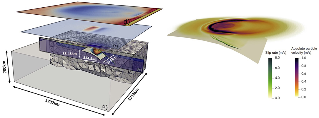
Figure 1. (Left): Adapted from Madden et al. (2020) (a) sketch and dimensions of the one-way linked 2D geodynamic subduction model, (b) the 3D dynamic rupture earthquake model, (c) the dynamic rupture seafloor displacement, and (d) the 2D tsunami model, modified from Madden et al. (2020). The 3D unstructured tetrahedral mesh of the dynamic rupture model (b) is shown in gray. (Right) Snapshot of slip rate across the 3D subducting interface (greenish colors) and the seismic wavefield recorded at the free surface in terms of absolute velocity (warm colors). This snapshot is extracted from model 3B after 40 s simulation time.

To link input and output data in massively parallel simulations, we use ASAGI (pArallel Server for Adaptive GeoInformation), an open source library with a simple interface to access Cartesian material and geographic datasets (Rettenberger et al., 2016, www.github.com/TUM-I5/ASAGI). ASAGI translates a snapshot of the 2D subduction model into 3D initial conditions for the earthquake model and bathymetry data and seafloor displacements from the earthquake model into initial conditions for the tsunami model. ASAGI organizes Cartesian data sets for dynamically adaptive simulations by automatically migrating the corresponding data tiles across compute nodes as required for efficient access.

2.1. 3D Earthquake Dynamic Rupture Modeling With SeisSol

Physics-based 3D earthquake modeling captures how faults yield, slide and interact (e.g., Ulrich et al., 2019a; Palgunadi et al., 2020) and can provide mechanically viable tsunami-source descriptions (Ryan et al., 2015; Ma and Nie, 2019; Ulrich et al., 2019b, 2020). We use SeisSol (de la Puente et al., 2009; Pelties et al., 2012, 2014) to solve simultaneously for frictional failure across prescribed fault surfaces and high-order accurate seismic wave propagation in space and time (illustrated in Figure 1, right). SeisSol uses a discontinuous Galerkin (DG) scheme with Arbitrary high-order DERivative (ADER) time stepping on unstructured tetrahedral grids with static mesh adaptivity (Dumbser and Käser, 2006; Käser and Dumbser, 2006). It is thereby particularly suited for modeling complex geometries such as those in the vicinity of subducting slabs. SeisSol is optimized for current petascale supercomputers (Breuer et al., 2014; Heinecke et al., 2014; Rettenberger et al., 2016; Uphoff and Bader, 2020; Dorozhinskii and Bader, 2021) and uses an efficient local time-stepping algorithm (Breuer et al., 2016; Uphoff et al., 2017; Wolf et al., 2020). Its accuracy is verified against a wide range of community benchmarks (Harris et al., 2011, 2018), including dipping and branching faults with heterogeneous off-fault material and initial on-fault stresses (Pelties et al., 2014; Wollherr et al., 2018; Gabriel et al., 2020). We note that on-fault initial conditions such as frictional parameters or initial fault stresses are assigned with sub-elemental resolution (at each DG Gaussian integration point). However, within each off-fault element, all material properties are constant. We create a 3D complex structural model in GoCad (Holding, 2018) and discretize it with the meshing software Simmodeler by Simmetrix (Simmetrix Inc., 2017).

Within SeisSol, frictional failure is treated as an internal boundary condition for which the numerical solution of the elastodynamic wave equation is modified. In the dynamic rupture scenarios of our study, fault strength, i.e., its yielding and subsequent frictional weakening, is governed by the widely adopted linear slip weakening (LSW) friction law (Ida, 1972). Over a critical slip weakening distance D_c the effective friction coefficient μ decreases linearly from static μ_s until reaching dynamic μ_d. We note that this is different to the rate-weakening friction used in the long-term geodynamic SC model. The process zone width is the inherent length scale defining the minimum resolution required on-fault, and is defined as the area behind the rupture tip in which shear stress decreases from its static to its dynamic value (Day et al., 2005).

2.2. Subduction Seismic Cycle Modeling for Earthquake Initial Conditions

Figure 2 depicts the inferred 3D initial conditions from the subduction seismic cycle model for all dynamic rupture scenarios. These include highly heterogeneous initial shear stress and strength as well as fault geometry and material structure that together govern earthquake nucleation, propagation, and arrest. The underlying 2D seismo-thermo-mechanical geodynamic seismic cycle (SC) model simulates subduction dynamics over millions of years and earthquake cycles over several hundreds of years (e.g., Van Dinther et al., 2013, 2014) (Figure 2A). The long-term phase of the simulation builds up stress as well as self-consistent strength and fault geometries across the subduction interface and forearc. The geodynamic SC model includes 70 megathrust events that rupture almost the entire fault and nucleate near the downdip seismogenic zone limit. The same representative event as in van Zelst et al. (2019) is here chosen and linked to the newly designed dynamic rupture model applying the techniques described in Madden et al. (2020). We note, that at the chosen SC time step, the dominant deformation mechanism in the seismogenic zone is elastic behavior, which is consistent with the deformation mechanism in the dynamic rupture model. All material properties, stresses, and fault geometries are exported from the SC model at that timestep. Material density and fault strength can be adapted to be used in the DR model. Cohesion varies between 2.5 and 20 MPa and increases with deeper lithologies. At nucleation depth, cohesion is set to 5 MPa. The curved, blind megathrust interface evolves during this slip event and is characterized by large-scale fault roughness including characteristic topographic highs (“bumps”) in terms of a distinct change in local gradients of the curved non-planar interface related to sediment intrusion on geodynamic time scales (zoom-in box of Figure 2A).

FIGURE 2

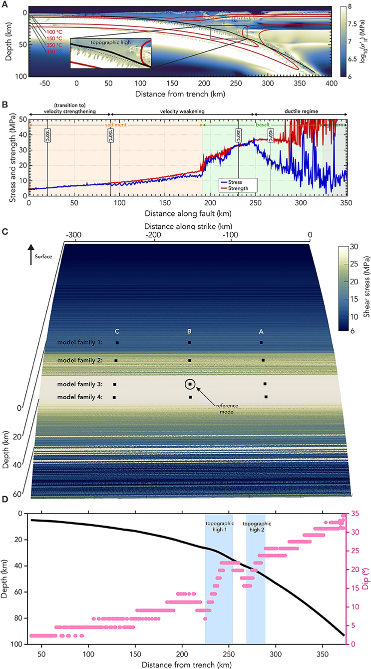
Figure 2. Subduction model initial conditions for the dynamic rupture earthquake simulations. (A) Snapshot of stresses evolving during the 2D long-term geodynamic subduction and seismic cycle simulation at the time-step right before a slip event occurs (adapted from van Zelst et al., 2019). The stresses are expanded to the third dimension assuming plane strain conditions. (B) On-fault shear stress and fault strength in the SC model at the coupling time-step. The fault yields and failure occurs when both align. (C) Pre-processed (see text) initial shear stress in the three-dimensional dynamic rupture model at timestep t = 0 s in the DR model. The black squares indicate nucleation locations that are used for model families 1–4. The hypocenter of the reference model 3B is marked. (D) Fault geometry in 2D and dip angle of the fault. Regions of increasing dip are highlighted in blue and indicate local topographic highs (1 and 2) in the fault plane.

In contrast to van Zelst et al. (2019) and Madden et al. (2020), the critical slip weakening distance D_c is here not inferred from the geodynamic SC model directly but is assigned to be a constant value (D_c = 0.1 m for 13 out of 14 dynamic rupture models) along the entire fault. Increasing the critical slip weakening distance D_c, over which effective friction is reduced to its dynamic value, results in a higher fracture energy G_c according to G_c = 1/2μ_sP_n−μ_dP_nD_c with P_n being the initial fault normal stress (Venkataraman and Kanamori, 2004). The fracture energy consumed within the frictional process zone indicates how much energy is necessary to initiate and sustain rupture propagation. A high fracture energy results in higher fault slip, higher stress drop and a higher moment magnitude for comparable dynamic rupture scenarios (given the nucleation energy is adopted accordingly). In one model, model 5, we triple the model-wide constant D_c from 0.1 to 0.3 m while keeping all other parameters constant, thus, tripling fracture energy.

All material properties are extrapolated into the third dimension as constant along arc, for simplicity. We use a plane strain assumption, as in the 2D subduction model, to determine the out-of-plane normal and shear stress components in 3D. This implies that we omit eventual oblique subduction components by setting the out-of-plane shear stresses to zero and the out-of-plane normal stress component to be a function of the two in-plane normal stresses and Poisson's ratio ν. In the SC subduction model a Poisson's ratio of ν = 0.5 is used, which is an appropriate assumption for large time scales. This Poisson's ratio needs to be reassigned within the DR model to represent compressible rocks and to solve the linear elastic wave equations. The choice of ν affects the material properties as they are transferred from the subduction model to the earthquake model since Lame's parameter is calculated from the re-assigned ν and the shear modulus G is taken from the subduction model. In all besides one dynamic rupture models we assume ν = 0.25 (Poisson solid, λ = G). In one 3D dynamic rupture (model 6, modified from reference model 3B), we use a larger Poisson's ratio of ν = 0.3, which is in the range observations of basaltic rocks (Gercek, 2007).

Using the imported on-fault conditions from the geodynamic SC model directly would lead to multiple locations of instantaneous failure on the fault (Figure 2B). We thus use a pre-processing static relaxation step in which we relax the initial fault loading stresses to be just below fault strength before applying them to the DR model following Wollherr (2018). Spontaneous earthquake rupture is commonly initialized by assigning an over-stressed or frictionally weaker predefined hypocentral “nucleation” area. We here assign a locally lower static friction coefficient within a circular patch of an empirically determined minimum required size to initiate spontaneous rupture. We choose frictional coefficients μ_s and μ_d within this patch constrained from the geodynamic SC model. We prescribe all but the shallowest (model family 1) hypocentral nucleation depths at locations which are close to failure (low strength excess, Figure 2B) in the SC model. The reference geodynamic SC slip event nucleates at 40 km depth, corresponding to model family 3 in this study.

2.3. Tsunami and Inundation Modeling With Samoa

Tsunami are modeled with a limited second order Runge-Kutta discontinuous Galerkin solver (Cockburn and Shu, 1998; Giraldo and Warburton, 2008) for the two dimensional depth-integrated hydrostatic non-linear Shallow Water Equations (SWE, LeVeque et al., 2011) in the sam(oa)²-flash framework (Madden et al., 2020). The SWE are a simplification of the incompressible Navier-Stokes equations, under the assumption that vertical scales are negligible compared to horizontal scales. As a result, hydro-static pressure and the conservation of mass and momentum are part of the equations, while vertical velocity and turbulence are neglected. Manning friction is included in the model with an additional source term (Liang and Marche, 2009). To allow accurate and robust wetting and drying, the model uses a Barth-Jaspersen type limiter that guarantees the conservation of steady states (well-balancedness), mass conservation and positivity preservation of the water-depth (Vater and Behrens, 2014; Vater et al., 2015, 2019).

The framework sam(oa)²-flash simulates hyperbolic PDEs on dynamically adaptive triangular meshes (Meister et al., 2016). It is based on the Sierpinsky Space filling curve, which allows cache efficient traversals of mesh-cells and -edges with a stack and stream approach. Cell-level adaptive mesh refinement in every time step and a water-depth based refinement criterion, allow for multiple levels of refinement for the tracking of wave fronts and other areas of interest (i.e., coasts). While tsunami are usually sourced by setting a perturbation to the seafloor and water surface as initial condition, sam(oa)²-flash can include the full spatio-temporal evolution of the seafloor displacement in the simulation. sam(oa)²-flash has been validated against a suite of benchmarks (Synolakis et al., 2008).

2.4. Dynamic Rupture Modeling for Tsunami Initial Conditions

The time-dependent seafloor displacement generated in the dynamic rupture model is used as input for the tsunami model. Since these displacements are written in form of a triangular unstructured grid by SeisSol, rasterization is required to obtain a regular grid that can be read by sam(oa)²-flash . The resulting grid is comprised of rectangular cells of size Δx× Δy= 500 m × 500 m. The geometric center of each cell is used to sample the triangular grid using a nearest-neighbor approach. Since all our examples share a relatively large source area and a short process-time, compared to the ocean depth (2 km), we here omit corrections required for landslide-induced tsunami (Kajiura, 1963) and neglect the effects of water flow from seafloor to sea-surface (Saito and Furumura, 2009; Wendt et al., 2009). We directly use the seafloor deformation as time-dependent (or static, for comparison) initial sea-surface perturbation.

The seafloor deformation data contains the seismic wavefield and the dominant static displacement, which remains unchanged after dynamic rupture propagation ceased since we do not account for post-seismic relaxation. Saito et al. (2019) shows that seismic waves have an effect on tsunami generation, but do not affect the solution in the far field. However, our earthquake scenarios also include reverberating seismic waves, e.g., trapped within the accretionary wedge. Simulating long enough for such complex seismic waves to stop imprinting on the time-dependent near-source seafloor deformation requires significantly longer simulation times. We here limit computational costs by stopping the DR earthquake simulation after the fault stopped slipping and the dominant static displacement remains constant. We apply the time-dependent seafloor deformation to source the tsunami model during that period and keep the seafloor elevation constant afterwards. In the presence of transient seismic waves, however, this approach may lead to artifacts such as spurious gravity-waves in the tsunami simulation. Thus, we here remove reverberating seismic waves using a filter-based approach on the seafloor perturbation.

We apply a Fourier filter approach that we base on an analytical test-bed in which we can separate the significant frequency-wavenumber coefficients of the permanent displacement from the ones of seismic waves (Madden et al., 2020). In the wavenumber representation for the displacement field we can identify the coefficients belonging to seismic waves clearly as radial symmetric lines in the wavenumber space (Supplementary Figure 1). Our analytical testbed confirms that these lines propagate in the frequency-wavenumber domain with the inverse velocity with which seismic waves propagate in time and space. Coefficients of the permanent displacement on the other hand are dominant close to the origin. To erase seismic waves from the seafloor perturbation we design a kernel to zero-out the radial symmetric waves in the frequency-wavenumber representation depending on their velocity. Close to the origin we leave the representation as it is, to keep the dominant coefficients of permanent displacement. To avoid rolling effects, the kernel is smoothed. As a result, seismic waves of chosen frequencies are effectively damped in the time-dependent displacement field (Supplementary Figure 2). The effects of seismic wave damping on the permanent displacement are negligible.

3. Earthquake and Tsunami Model Setup

3.1. 3D Heterogeneous Megathrust Dynamic Rupture Models

In DR modeling, rupture can only propagate across predefined fault interfaces. In distinction, fault geometry spontaneously arises during slip events in the SC model. The fault geometry for the chosen slip event at the coupling time step is shown in Figure 2A. The locations of the highest visco-plastic strain rate represent the fault. A moving average scheme is used to smooth this 2D fault geometry, which is then uniformly extruded along-arc to construct the 3D DR fault plane (van Zelst et al., 2019; Madden et al., 2020). The 3D dynamic rupture fault (Figure 2C) does not intersect the surface but ends ≈5 km below the seafloor and extends to 93.5 km depth. The fault length in the along-arc y-direction is chosen to agree with the average scaling of the source dimensions of interface and intraslab subduction-zone earthquakes with moment magnitude (Strasser et al., 2010). We here aim to model typical size tsunamigenic earthquakes of magnitudes close to M_W=8.5, and thus choose a fault width of ≈313 km. The curved fault is characterized by large scale roughness. Noticeable are two topographic highs shown in terms of sharp increases of fault dip in Figure 2D. We use a constant element edge length of 1 km along the fault. We ensure that this element size along the fault is sufficient to capture the median process zone width following all error criteria of Day et al. (2005) in a series of models with different size elements following the analysis in Wollherr et al. (2018). We measure the median process zone width as 1,386 m for the reference model 3B and 1,224 m for model 1B. For a polynomial basis function of order p = 5 (Wollherr et al., 2018) estimate the minimum required resolution to be 1.65 elements per median process zone width. A polynomial basis function of p = 5 leads to 6th order numerical accuracy in space and time in the seismic wave propagation solution. We note that each tetrahedral element fault interface is discretized by (p+2)² Gaussian points. In Supplementary Figure 3 we detail two exemplary higher resolution versions (h=500 m, p=5) of the reference model 3B and of model 1B which has the shortest median process zone width. Compared to the coarser resolution of h = 1 km, we quantify the error to be <1% for the maximum vertical seafloor displacement, <6% for the rupture velocity, <5% for the average peak slip rate and <2.5% for the average fault slip which agree with the criteria for well-resolved models by Day et al. (2005). We note that in contrast to the simple depth-dependent setup in Wollherr et al. (2018), the peak slip rate and not the average fault slip is most sensitive here.

The 3D model domain extends from x = −657 to x = 1,075 km and y = −1,023 to y = 700 km and to a depth of z = −700 km. The large model size prevents that waves reflected from non-perfect absorbing boundary conditions interfere with the rupture itself. To limit computational cost, the unstructured tetrahedral mesh is statically coarsened. The sea floor is flat in the DR model (but not in the tsunami simulations) and assigned a free surface boundary condition. The mesh size is 7.8 million elements. Each simulation took 1:10 h on 75 nodes, with 48 Intel Xeon Skylake cores each, of Supermuc-NG.

To analyze the effects of material directivity and complex initial conditions, as well as uni- and bilateral rupture behavior in the DR models, and the resulting tsunami, we vary the hypocenter location along arc and depth. We choose fault locations which are close to failure in the 2D SC model, at 30, 40, and 45 km depth (Figure 2B). To analyze shallower earthquake nucleation locations, we additionally nucleate 3D DR scenarios at 25 km depth (Figure 2C). The reference dynamic rupture model (Model 3B) is nucleated at the origin location of the slip event in the SC model, that is, at a depth of 40 km and at the center of the fault along strike (x = 267.25 km, y = −156.5 km). The static friction coefficient is reduced to μ_s = 0.019 within a patch of radius 2 km, which represents the minimum value in the SC model within the nucleation area (Table 1). For all earthquake model families, the assigned nucleation parameters, that is locally reduced static friction coefficients μ_s and patch radii r, are listed in Table 1. To evaluate effects in lateral direction, we move the hypocenter from y = −156.5 km (fault width center) to y = −78.25 km (25% of the fault width) and y = −234.75 km (75% of the fault width), exploring observational and statistical inferences of large ruptures being predominantly unilateral or bilateral (McGuire et al., 2002; Mai et al., 2005) (see Figure 2C). We note that larger nucleation energy (larger radii, lower local strength) are required in fault regions further from failure than the reference model (hypocentral depth of 40 km).

TABLE 1

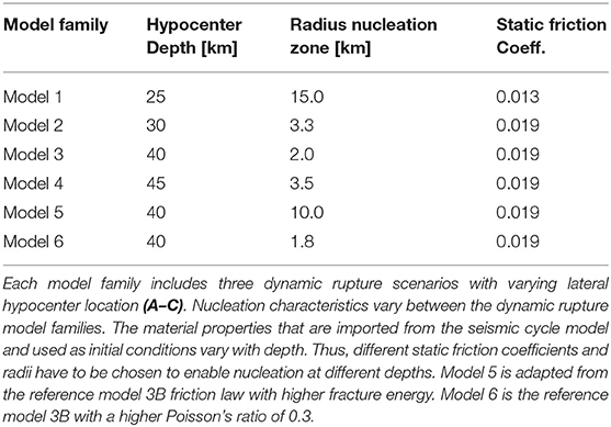
Table 1. Model families 1–4 defined by hypocentral location.

3.2. Tsunami Model Setup

The tsunami modeling area extends from x = −600 to x = 600 km and from y = −750 to y = 450 km, the ocean depth being at a constant 2 km. A linearly sloping beach is placed with its toe at x = 500 km with an inclination of 5%, which results in the coastline being located at x = 540 km in most models (see Figure 3, left). We additionally analyze the inundation behavior along a more realistic coastline in one model (model 4D). To this end a non-linear coastline is included in model 3B (Figure 3, right). We adapt the coastal topo-bathymetry of the Okushiri benchmark (Yeh, 1996; Honal and Rannabauer, 2020) and stretch it along the full y-direction model length. Every tsunami is generated using the time-dependent (dynamic) seafloor displacements generated in the 3D DR models from 0 to 200 s.

FIGURE 3

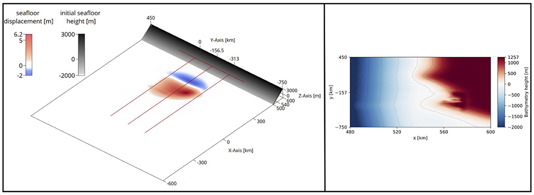
Figure 3. (Left) Sketch of the tsunami model setup for most scenarios for sam(oa)²-flash with a linearly sloping beach starting at x = 500 km. Red and blue colors are an exemplary snapshot of seafloor uplift and subsidence resulting from a DR model that are used to source the tsunami model. (Right) Zoom-in of the non-linear height profile of the complex beach used in one tsunami scenario (model 4.D) adapted from the Okushiri benchmark. The position and slope are designed to be comparable to the linear beach (left). The depth profile is illustrated by blue and red colors. Contour lines are shown every 500 m.

Depending on the used DR model setups, different tsunami modeling refinement levels and output configurations are required. The minimum spatial resolution in sam(oa)²-flash is defined as Δx = domain-width·(1/2)^d/2. We use a minimum refinement level of d = 18 for all tsunami simulation runs, yielding a minimum spatial resolution of Δx = 2.34 km. To obtain detailed inundation patterns, we use a refinement of d = 30 (Δx = 36.62 m) near the coast and a maximum refinement of d = 26 (Δx = 146.5 m) in the remainder of the domain. On SuperMUC-NG, these simulations took 2:43 h on 100 nodes sourced by dynamic displacement. This corresponds to roughly 13,000 CPUh, respectively. Simulation outputs are in general written every 10 s of simulation time. If only sea surface height tracing measurements along a few axes are needed, a run with a maximum refinement of d = 24 (Δx = 293.0 m) takes approximately 27 min across 100 nodes (2,187 CPUh) with dynamic displacement. Output of the full wavefield with a maximum of d = 24 took 1:21 h across 32 nodes (2,074 CPUh) for dynamic displacements, writing outputs every 100 s of simulation time between t = 0 and t = 3,000. We note that in all our tsunami models, including a slow “tsunami earthquake,” the ratio of tsunami source width/ (source time × tsunami wave speed), in water depth of 2 km is >>1, indicating that the tsunami does not propagate over the source duration (Abrahams et al., 2021). We find differences of up to 10% in the tsunami system energy balance of kinetic and potential energy when comparing static with dynamic sources and source all tsunami in the following from the dynamic seafloor displacement.

4. Results

4.1. Dynamic Rupture Models

We first investigate the effects of varying earthquake hypocenter locations in complex subduction initialized dynamic rupture models. We vary the hypocentral depth between 25, 30, 40, and 45 km, which resembles one shallow earthquake and three low strength excess regions in the geodynamic subduction and seismic cycle model. It has been inferred that hypocenters of large earthquakes are not arbitrarily distributed across fault planes, but located close by regions of large slip (Mai et al., 2005). Additionally, large subduction zone events may propagate preferably unilateral (McGuire et al., 2002) or bilateral (Mai et al., 2005) and rupture dynamics of subduction earthquakes may be significantly affected by bimaterial contrasts (Ma and Beroza, 2008). In our 12 scenarios listed in Table 1, different hypocenter depths lead to pronounced differences in dynamic rupture propagation. The models differ in their propagation direction, slip rates and rupture velocities, and include localized supershear rupture at different simulation times and fault locations.

Figures 4–6 compare snapshots of slip rate and rupture velocity as well as the accumulated fault slip of all 12 models. Animations of slip rate are provided in the Supplementary Material. Supplementary Figure 4 shows the peak slip rate of all 12 models. Table 2 summarizes all rupture characteristics.

FIGURE 4

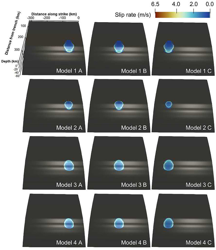
Figure 4. Slip rate at the timestep t = 12 s (model 1), t = 16 s (model 2), t = 10 s (model 3), and t = 14 s (model 4), capturing down-dip and up-dip propagating supershear rupture being triggered by one of the two topographic highs in the fault geometry depending on hypocentral depth. The white reflections highlight the uneven geometry of the fault. The hypocentral locations vary with depth (25, 30, 40, and 45 km) and laterally on the fault (y = −78.25 km, y = −156.5 km, y = −234.75 km). For model 1 and 2 supershear rupture evolves in downdip direction, whereas for model 3 and 4 in updip direction.

TABLE 2

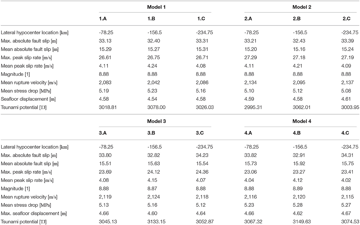
Table 2. Dynamic rupture and tsunami characteristics for model 1–4 with centered and lateral varying hypocenter locations.

In model family 1 (shallowest hypocenter) nucleation is initiated at a depth of 25 km which is located above topographic high 1 on the megathrust. We observe complex dynamic rupture behavior, including supershear transition at topographic high 2, localized high slip rates within the fault depression and reactivation of fault slip at a late stage. Rupture propagates at low slip rates before reaching the edge of the first topographic high, where the slip rate increases. As the main rupture front hits the second topographic high (10 s), supershear rupture initiates in downdip direction (Figure 4).

For model family 2, we observe complex downdip propagating dynamic rupture behavior with supershear rupture being triggered at the second topographic high. The hypocenter is located at the edge of topographic high 1 (Figure 2). As the rupture front passes topographic high 1, slip rate increases, similar to model family 1. Supershear rupture is triggered in downdip direction at 15 s simulation time (Figures 4, 5).

FIGURE 5

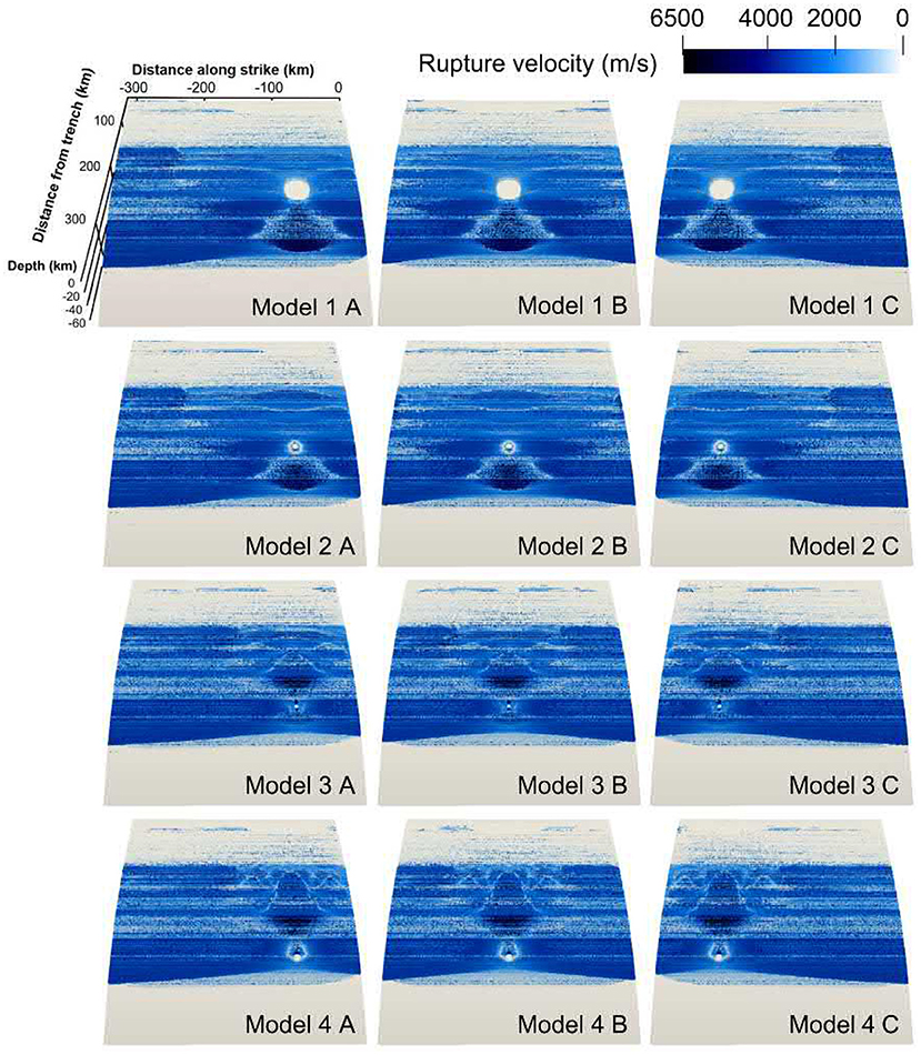
Figure 5. Rupture velocity for 12 dynamic rupture simulations with varying hypocenter locations. Note the difference in nucleation radii according to Table 1. Most parts of the fault rupture at speeds around 3,000 m/s. Much lower velocities are visible in the shallower fault part. Supershear rupture is visible as dark blue areas in downdip direction for nucleation locations at a depth of 25 and 30 km and in updip direction for nucleation depths of 40 and 45 km. The rupture velocity is very inhomogeneous due to the complex and heterogeneous material properties on the fault.

The nucleation location in model family 3 corresponds to spontaneous failure in the 2D SC model. It is located on the lowermost point of the geometric depression of the fault, at 40 km depth. Slip evolves circularly and propagates away from the hypocenter. After 8 s simulation time, supershear rupture initiates in updip direction at topographic high 1 (see Figures 4, 5).

For model family 4, the hypocenter was placed at a depth of 45 km, which lies at the edge of the second topographic high. A circular rupture front evolves during 9 s simulation time. Supershear rupture arises in updip direction after 13 s, when the rupture front hits the first topographic high (Figures 4, 5).

In all 12 models, rupture fronts reach the lower limit of the seismogenic zone at x = 282.25 km after passing the second topographic high. In the SC model, ductile behavior begins to dominate here which is expressed as strength increase in the DR model. Rupture propagation is spontaneously arrested at this depth. Thus, in all 12 models, slip stops at the same depth. At the lateral edges of the prescribed megathrust fault, rupture is geometrically stopped, and no tapering of initial stress or strength is applied. Close to the surface, in the shallowest part of the fault, the sedimentary region allows for small slip while smoothly stopping rupture.

Bilateral rupture evolution appears to be symmetrical for centered hypocenters, despite bimaterial contrasts above and beneath the fault potentially affecting strike-slip faulting contributions (Harris and Day, 2005). For asymmetric hypocenter locations (models A and C of each model family), unilateral dynamic rupture propagation is identical to bilateral models within the first seconds until stopping phases from the closer fault edge affect rupture dynamics. In both cases (A and C), rupture dynamics appear minor symmetric with slight bimaterial effects (see rupture characteristics summarized in Table 2). Larger slip is accumulated at the respective far side of the fault (Figure 6). The highest absolute slip is observed in the models with hypocenter locations at y = −234.75 km (C models) and the lowest absolute fault slip is observed for models with hypocenters placed in the center of the fault (B models).

FIGURE 6

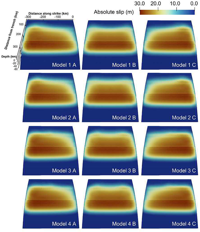
Figure 6. Accumulated fault slip at the end of the simulation, after 200 s for 12 dynamic rupture models. The hypocenter locations vary with depth (25, 30, 40, and 45 km) and laterally on the fault (y = −78.25 km, y = −156.5 km, y = −234.75 km).

In all 12 models we observe localized weak reactivation of slip after approximately 100 s simulation time due to dynamic triggering caused by trapped waves. Waves are trapped within the accretionary wedge between the uppermost part of the fault and the surface until the end of the simulation (200 s). They are reflected at the free surface boundary and propagate back to the fault, which leads to very small amounts of shallow slip in the order of centimeters. As noted before, in the tsunami linking step any artificial contribution of these waves to seafloor displacements will be filtered.

Across all 12 models, the highest peak slip rate (PSR) occurs on the lower part of the fault, inside the geometric depression at ≈40 km depth, and spread out in along-strike direction (Supplementary Figure 4, Table 2). Model family 2 produces the highest PSR (model 2A, 27.29 m/s). Deeper earthquakes produce lower peak slip rates, such that the earthquakes with the deepest hypocenter (model family 4) exhibits the lowest PSR (model 4A, 23.06 m/s). Along-arc, PSR first increases while rupture propagates away from the hypocenter. Then it decreases due to dynamic interaction with the free surface and other fault edges. At the hypocenter, the PSR is low.

The overall highest absolute slip of 34.31 m is observed for model 4C (see Table 2) and the lowest absolute fault slip is observed for model 1B (32.40 m). For models with the same hypocentral depth, the maximum accumulated fault slip is consistently observed when the hypocenter location is located laterally at y = −234.75 km. At the same time, these earthquakes show relatively low peak slip rates. The lowest maximum absolute fault slip for models with the same hypocenter depth is observed for a laterally centered hypocenter. Moment magnitudes vary from M_W = 8.87 (model 3B) to M_W = 8.89 (model 4B, Table 2).

4.2. Tsunami Simulations

At 200 s simulation time, the filtered vertical sea-surface uplift has a maximum of ≈4 m which is located above the buried dynamic rupture fault plane for all 12 models (see Supplementary Figure 5). The sea surface uplift and subsidence reflect the patterns of accumulated slip in Figure 6. Thus, despite the stark dynamic differences in rupture dynamics between the 12 models, including supershear rupture evolution in up- or downdip direction, the static sea surface disturbance is nearly the same. For models of one family, we see lateral differences in the spatial extend of the sea surface uplift which are related to laterally varying hypocenter locations. For models with asymmetric on-fault slip distributions, we observe the same pattern in the sea surface uplift.

Supplementary Figure 6 illustrates the dynamically sourced tsunami propagation toward the simulation domain boundaries. After 2,300 s simulation time, the tsunami arrive at the coast with wave heights of up to ≈5.5 m. At the coast, we observe differences in the tsunami arrival times for laterally varying hypocenter locations of up to 100 s (Figure 7). The time delay between the tsunami waves caused by an earthquake with a centered hypocenter (B) and an earthquake with a hypocenter located at y = −78.25 km (A) are always some tens of seconds higher than the time delay between events with a centered hypocenter (B) and a hypocenter location of y = −234.75 km (C) (see Supplementary Figures 7–9). We observe only insignificant differences in the tsunami arrival time at the coast with varying hypocentral depths (Supplementary Figures 10–12). Tsunami that were generated by deeper earthquakes arrive few seconds later than those being generated by shallower ones.

Figure 7 shows the sea surface height (ssh) of the tsunami when arriving at the coast. We observe non-symmetric differences in coastal ssh in dependence of earthquake along-strike hypocentral location. A maximum wave height of ≈5.5 m can be observed in all 12 simulations. The difference in the tsunami height (Δssh) of models with a centered hypocentral location (B) and a hypocenter located at y = −78.25 km (A) present higher values of approximately 0.25–0.4 m than the Δssh of earthquakes with a centered hypocenter location (B) and earthquakes located at y = −234.75 km (C) (Δssh is ≈ 0.1 m). This agrees with the differences in tsunami arrival at the coast. For larger time delays we observe larger differences in the tsunami height accordingly. In summary, comparing all model families 1A-C, 2A-C, 3A-C, and 4A-C, the largest difference of 6 cm in coastal sea-surface heights can be observed between the shallowest earthquakes (models 1A-C) and earthquakes nucleating at 40 km depth (models 3A-C) (see Supplementary Figures 13–18).

FIGURE 7

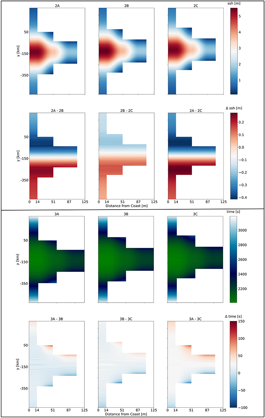
Figure 7. (Top) Comparison of sea surface height (ssh) for tsunami fronts arriving at the coast for the models 2A–2C (upper row). The difference in arrival times between the models is shown as Δssh (lower row). (Bottom) Inundation comparison for models 3A–3C. The green to white color scale shows the time delay for the tsunami fronts arriving at the coast (upper row). The difference in inundation between respective models is plotted as Δt (lower row).

We calculate the potential energy transferred by the earthquake rupture to the sea surface (the “tsunami potential energy”) (Melgar et al., 2019; Crempien et al., 2020):

$\begin{array}{ll}{E}_T=\frac{1}{2}\rho g{\displaystyle \int }{\displaystyle {\int }_A}{\eta }^{2}dA,& (1)\end{array}$

where η is the vertical, static sea-floor deformation of the DR model (corresponding to the sea surface heights after 200 s shown in Tables 2, 3), with a water density of ρ=1,000kg/m³ and the gravitational acceleration being g=10m/s. The deepest earthquake (model 4B) produces the highest tsunami potential with ≈3,150 TJ which marginally differs from the tsunami potential of model 3B (Table 2). The tsunami resulting from shallower hypocenter depths (models 1B and 2B) have slightly smaller tsunami potentials of 3,078 and 3,062 TJ. Within model families 1 and 2, a centered hypocenter location leads to the highest tsunami potential, while for model family 3 and 4, the centered hypocenter causes the smallest tsunami potential. Within each model family, tsunami simulations with a hypocenter location at y = −78.25 km (A) always present lower tsunami potentials than models with hypocenter locations at y = −234.75 km (C).

TABLE 3

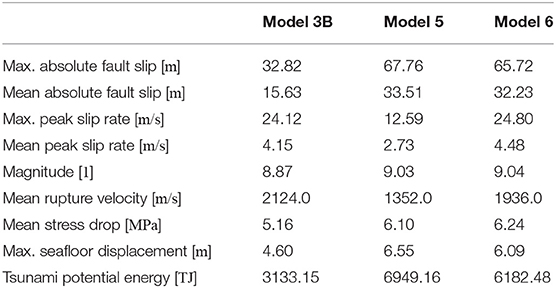
Table 3. Dynamic rupture and tsunami characteristics for model 3B, 5, and 6 with centered hypocenter locations.

4.3. Tsunami Simulation With Complex Coastal Topo-Bathymetry

We perform an additional tsunami simulation, model 3D, which is adapting model 3B by replacing the linearly sloping beach with a complex coastline (see Figure 3, right). We adapt the coastal topo-bathymetry of the Okushiri benchmark (Honal and Rannabauer, 2020) and stretch it along the full y-direction model length (section 3.2). The resulting sea-surface height and inundation area are displayed in Figure 8. Tsunami inundation is observed along the entire length of the coast. While the coastal parts at the far-ends of the domain are hit by a shallow wave of approximately 1 or 2 m, its central part is hit by high wave amplitudes of up to 8 m. In this model, the tsunami amplitudes are ≈2.5 m higher, compared to absolute sea-surface heights of ≈5.5 m for the linearly sloping beach.

FIGURE 8

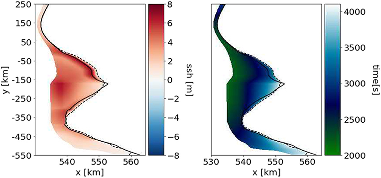
Figure 8. Sea-surface height of the waves at the coast (left) and inundation area and time (right) for the tsunami scenario with a complex coast (Figure 3, right). Note the different x-axis scale compared to Figure 7 which is necessary to resolve the complex coastline at the beginning of the simulation (solid black line) accurately. The dotted line illustrates how far in-land the tsunami inundates.

4.4. Simulations With Increased Fracture Energy and Poisson's Ratio

We here analyse two additional dynamic rupture models based on reference model 3B varying on-fault or off-fault rheology. Firstly, we triple the critical slip weakening distance D_c from 0.1 to 0.3 m (model 5) which triples fracture energy and generates a “tsunami earthquake.” Secondly, Poisson's ratio is increased from ν=0.25 to ν=0.3 (model 6) everywhere in the domain. Both models result in shallow slip about twice as high as the reference model 3B (see Table 3). Table 1 shows the adapted nucleation characteristics that were necessary to initiate rupture on the fault. We do not further decrease the static friction coefficient, but increase the nucleation radius from 3.5 to 10.0 km (model 5). In model 6 a smaller nucleation area of only 1.8 km is sufficient. For the high fracture energy model 5, rupture dynamics evolve very differently to model 3B, specifically at much lower rupture velocities of max. 1,352 m/s. There is no supershear rupture triggered during the entire simulation time. In model 6 the dynamic rupture evolution is similar to model 3B and supershear rupture evolves in updip direction after 9 s.

For both models, 5 and 6, trapped waves are observed until the end of the simulation (200 s) dynamically interacting with the shallow part of the fault.

Figure 9 displays the rupture characteristics of model 3B, model 5, and model 6. Compared to the reference model 3B, both adapted models accumulate large shallow slip. The maximum and average fault slip of models 5 and 6 are about twice as high as in the reference model 3B (see Table 3), which reflects in increased earthquake magnitudes of M_W=9.03 (model 5) and M_W=9.04 (model 6). Also, their dynamic stress drops are higher and the maximum vertical dynamic seafloor displacement is increased by up to ≈2 m. Model 5 shows a much smaller PSR (12.59 m/s) and rupture velocity (1,352 m/s) then model 3B (24.12 and 2,124 m/s), while the PSR (24.80 m/s) and rupture velocity (1,936 m/s) of model 6 are similar to the reference model. The maximum PSR for all three models is always observed at the same depth which is located within the fault depression at ≈40 km depth.

FIGURE 9

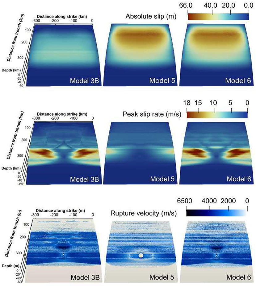
Figure 9. Fault slip, peak slip rate, and rupture velocity for the dynamic rupture models 3, 5 (increased fracture energy), and 6 (higher Poisson's ratio) after 200 s at the end of the DR simulation.

Figure 10, top, compares the sea-surface height of models 5 and 6 after 200 s, corresponding to the end time of the DR simulation. The overall tsunami waveforms in models 5 and 6 appear to be broader than in model 3B (Supplementary Figure 7) and the trajectories in Figure 10, bottom, show much higher tsunami amplitudes. After 1,400 s simulation time, the wave amplitudes of model 3B reach extrema of +2 and −3 m, whereas the tsunami in models 5 and 6 reach values of +2 and −5 m. After 2,300 s simulation time, the wavefronts hit the coast and result in maximum tsunami heights of over 7.5 m. This is ≈2.0 m higher than in the reference model 3B. An important difference between models 5 and 6 is the difference in rupture speed. While model 6 produces supershear rupture, the overall rupture velocity of model 5 is ≈1,352 m/s. Thus, although the model 5 earthquake scenario has a slightly smaller stress drop and magnitude than model 6, it produces the highest tsunami amplitudes.

FIGURE 10

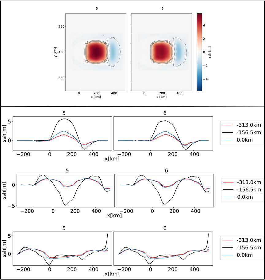
Figure 10. (Top) Sea surface height (ssh) for models 5 and 6 at t = 200 s with contours at −0.5, 0.5, 1.0, and 1.5 m, at the end of the DR earthquake simulations. (Bottom) Trajectories of the sea surface height for dynamically sourced tsunami (model 5 and 6) measured at y = 0.0, −156.5, and −313.0 km. Directly after the earthquake at t = 200 s (top), during the wave propagation at 1,400 s (middle), and at the time of coastal inundation at t = 2,200 s (bottom).

As the waves hit the coast there is a time delay of 100 s and a difference in tsunami height of ≈0.5 m between models 6 and 5 (see Figure 11). Due to the overall higher tsunami waves of models 5 and 6, the water inundates further on-shore and reaches higher distances from the coast than for model 3B. Model 5 has the highest tsunami potential with roughly 6,950 TJ and model 6 has a tsunami potential of 6182.48 TJ (Table 3). The tsunami potential of model 5 is twice as high as the one of reference model 3B.

FIGURE 11

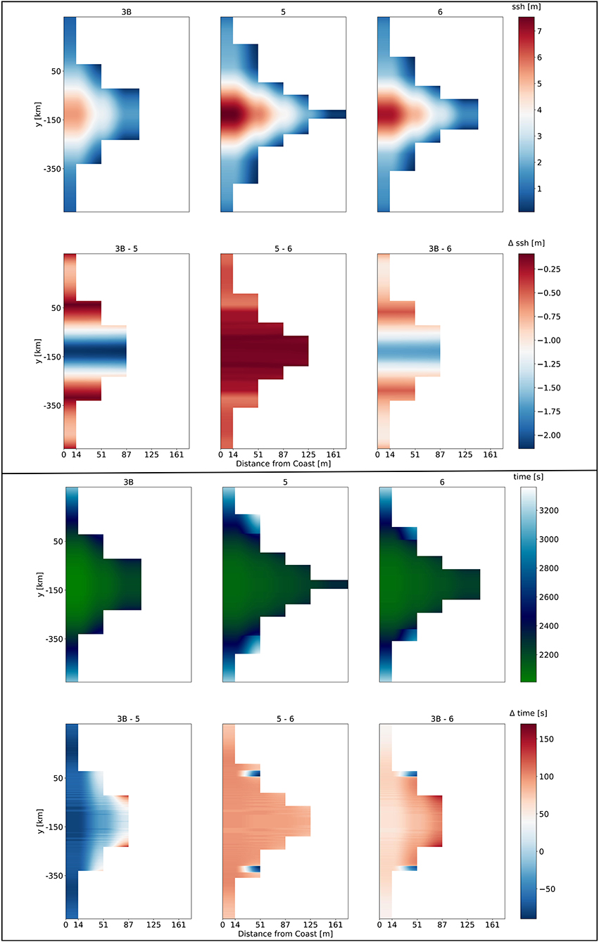
Figure 11. (Top) Comparison of sea surface height for tsunami fronts arriving at the coast for the models 3B, 5, and 6. The difference between the models is shown as Δssh. In contrast to Figure 11 the x-axis (distance from coast) indicates higher values. This is due to the greater inundation area of model 5 which exceeds 161 m distance. (Bottom) Inundation comparison for models 3B, 5, and 6. The green to white color scale shows the time delay for the wave fronts arriving at the coast. The difference between the models is plotted as Δt with a blue (negative values) to red (p color-scale, respectively.

4.5. Dynamic Effects During Tsunami Generation by Supershear and Tsunami Earthquakes

Figure 12, top, shows snapshots of the unfiltered DR seafloor displacements of models 1B (supershear rupture in downdip direction), 3B (supershear rupture in updip direction), and 5 (tsunami earthquake, no supershear rupture) after 100 s simulation time. Localized, sharp uplifting fronts are visible in the dynamic displacement off-set from the centrally located hypocenter overprinting the static deformation signal. The ocean response recorded within the source region during the tsunami generation process of all 3 models (Figure 12, bottom) reflect the seismic, and near-field displacements around a rupture front at 100 s simulation time. The time series shown is recorded at x = −100 km and y = −150 km, which is well inside the DR modeling domain.

FIGURE 12

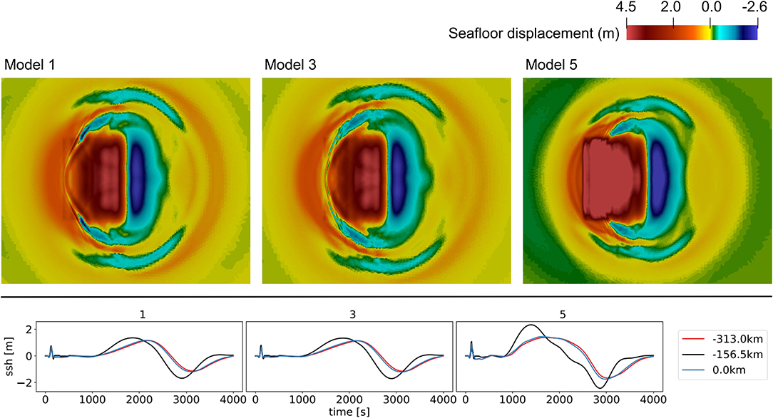
Figure 12. (Top) Unfiltered seafloor displacements from dynamic rupture model 1B (supershear rupture in downdip direction), 3B (supershear rupture in updip direction), and 5 (tsunami earthquake) at a simulation time of 100 s. (Bottom) Tsunami generation sea surface height timeseries for model 1B, 3B, and 5 at x = −100 km, y = −150 km.

In our models, co-seismic ocean response phases appear for supershear earthquakes as well as for the “tsunami earthquake” propagating at sub-Rayleigh speed during the duration of earthquake slip and within the DR model, i.e., for the dynamic tsunami generation process. We here do not observe a faster, instantaneous supershear mach cone ocean response signature (e.g., identified in Elbanna et al. (2020) for strike-slip events). Additionally, due to our filtering approach, trapped seismic waves are effectively damped, also inside the near-fault region once rupture stops. We then do not observe dynamic phases propagating (Supplementary Figures 5, 6).

5. Discussion

5.1. Simplifying Model Assumptions

In this study, we link 3D dynamic rupture initial conditions to a chosen slip event in a 2D long-term geodynamic subduction and seismic cycle. The linked initial conditions include a curved, blind fault geometry, spatially heterogeneous fault stresses, strength, and material properties. The SC 2D material properties, fault geometry, as well as stresses and strength are extruded into the third dimension without adding additional along-strike variability. While limiting complexity, we can in this manner isolate sensitivities, e.g., of hypocentral location, and their effects on rupture dynamics and tsunami generation, propagation and inundation.

In linking from the SC to the DR model, we adopt several simplifying assumptions to bridge the incompressibility and visco-elasto-plastic, plane-strain conditions of the subduction model to the compressible, elastic conditions of the earthquake model. The resulting 3D dynamic rupture is linked with the tsunami model through the time-dependent seafloor displacements, following the same methods as detailed in Madden et al. (2020). All resulting rupture models are characterized by uniformity along strike, rendering the dynamic earthquake source differences to be associated with along-dip variability in rupture dynamics controlled by the nucleation position relative to the two bands of topography on the megathrust. Future work may extend our analysis to include along-arc variations in stress, strength, rheology, and geometry across the megathrust as suggested by detailed imaging of fault geometry and shown to impact earthquake and tsunami dynamics (e.g., Galvez et al., 2019; Ulrich et al., 2020). The adopted “bumpy” fault geometry develops self-consistently with stress, strength and rheology in the SC model. Its along-depth dimensions aligns with conceptual asperity models governing megathrust fault slip. Future work may study the dynamic effects of subducted seamounts (e.g., Cloos, 1992) ensuring to adapt initial stresses consistently.

We use fully elastic material response in combination with linear slip weakening friction. The complexity of the DR model could be increased by including more complex physics, such as rapid velocity weakening rate-and state friction (Ulrich et al., 2019a), thermal pressurization of pore fluids (Gabriel et al., 2020), or off-fault plasticity (Wollherr et al., 2018; Ma and Nie, 2019).

In the linking step from the DR model to the tsunami model, we filter the seafloor displacements using a spatial-temporal Fourier-transform (section 4.5). Detailed analysis of the effects of relatively small coseismic phases on tsunami genesis, propagation, and inundation is here challenging due to the filter we apply. Future studies may use the unfiltered seafloor displacement as input to the tsunami model to analyse the fully dynamic interaction of the seafloor movements with the tsunami and inundation dynamics. sam(oa)²-flash 's hydrostatic shallow water tsunami model enables the simulation of tsunami genesis, propagation, and inundation at the coast. The approach is limited by the assumption of long wavelengths. Additionally, it does not take the interaction of wind with the water interface into account. Overall, the usage of the shallow water equations might overestimate wave amplitudes.

Our DR models do not account for seafloor bathymetry. A more realistic bathymetry would translate the horizontal earthquake motion into vertical displacements, such that the tsunami amplitude might be amplified (Tanioka and Satake, 1996; Lotto et al., 2018; Saito et al., 2019; Ulrich et al., 2019a). Recent work in van Zelst et al. (2021) complement this paper by using the exact subduction bathymetry and topography arising from the 2D seismic cycle model and include it in 2D DR simulation. The resulting seafloor displacement is linked to a one-dimensional shallow water tsunami model. The resulting maximum tsunami amplitude is 6.5 m, larger than our comparable 3D reference model 3B. It is here left for future work to combine their findings with our 3D sensitivity analysis.

The computational costs of each of the presented 15 linked scenarios (see sections 3.1 and 3.2) is well within the scope of the allocation typically available to users of supercomputing centers. While hundreds of such simulations are readily possible, fully physics-based dynamic rupture models rather complement than replace cheaper (e.g., kinematic) source descriptions used for millions of PTHA forward models. Specifically, for narrowing down the high-dimensional and often non-unique source parameter space in conjunction with observational or long-term modeling constraints and for sensitivity analysis of other parameters influencing rupture behavior and tsunami generation and propagation.

5.2. Hypocentral Depth and Up-Dip vs. Down-Dip Supershear Rupture Propagation

We vary the hypocenter location across four depths (25, 30, 40, 45 km) to study the effects on rupture dynamics and tsunami evolution, propagation, and coastal inundation. Earthquakes with shallower hypocentral depths (25 and 30 km depth) generally generate lower slip than earthquakes with deeper hypocenters (40 and 45 km depth). The lower accumulated on-fault slip for events with shallower hypocenters leads to comparably lower vertical seafloor displacement. In our SC initialized models, however, these differences are relatively minor and have small impact on tsunami generation, propagation and inundation, in contrast to what is typically observed from observational data (Bilek and Lay, 2018).

For simulations with shallower hypocenter locations, we observe supershear rupture propagating in the downdip direction, while hypocenters located at 40 and 45 km depth lead to supershear rupture in the updip direction. In either case, the slab geometry (topographic highs) and rheology influences the nucleation and direction of supershear rupture propagation significantly. In all our simulations, supershear rupture initiates when the rupture front hits a topographic high on the fault plane. The first topographic high (1) is related to a pile up of subducted sediments. The weaker material at the depth of the topographic high 1 might facilitate supershear rupture. Supershear rupture is also triggered by the second topographic high highlighting the complex dynamic effects of the long-term self-consistently developing fault roughness, stress, and rheology heterogeneities. The direction of supershear rupture propagation is determined by whether the updip or downdip rupture front interacts with the rough fault geometry (Bruhat et al., 2016; Bao et al., 2019; Tadapansawut et al., 2021). Megathrust supershear rupture is challenging to identify observationally but has been suggested in back-projection analysis of the Tohoku-Oki megathrust earthquake (Meng et al., 2011) and was analyzed in Cascadia 2D dynamic rupture models by Ramos and Huang (2019) who observe down-dip supershear rupture propagation near the ETS region caused by normal stress gradients (similar to the conditions governing our topographic highs).

Independent of where the earthquakes nucleate, the highest peak slip rate is consistently observed at the same location on the fault: inside the depression that separates the two local fault topographic highs, although the intensity of the slip rate decreases with increasing hypocentral depth. The calculated tsunami potential energy varies in the range of ΔE_T≈78 TJ for earthquakes nucleating at different depths. This is caused by a difference in the maximum seafloor displacement of approx. Δ=0.13 m.

5.3. Bilateral vs. Unilateral Rupture on a Complex Bimaterial Megathrust

To study unilateral vs. bilateral rupture effects on rupture dynamics (Hirano, 2019; McGuire et al., 2002) and tsunami generation, we shifted rupture nucleation from a centered hypocenter to 25% (A) and 75% (C) of the fault width (y = −78,25 and y = −234,75 km). Overall, differences are small. However, we note that earthquakes with a centered hypocentral location (B) consistently produce the highest stress drops and lowest accumulated slip on the fault, which lead to the lowest vertical seafloor displacement. The simulations with a nucleation patch at 75% (C) of the fault width show the highest accumulated slip for earthquakes at the same depth, but relatively low PSR. Due to the high amount of accumulated slip, we would expect the seafloor displacement to be the highest as well, but this is not the case for all model families, due to bimaterial effects (Brietzke et al., 2009). These effects lead to (minor) differences in amplitudes of the resulting tsunami at the coast and the (short) time delay between the arriving wave fronts. The higher sea surface uplift is also seen in the trajectories of the different models (Supplementary Figure 7).

We note again, that in difference to Madden et al. (2020), we here use the 2D geodynamic SC model developed in van Zelst et al. (2019) which has twice larger shear moduli. All our earthquakes show a higher stress drop of roughly 5 MPa compared to 2.2 MPa in Madden et al. (2020), whereas the rupture velocity remains the same (≈2, 100m/s). They also show a comparably lower maximum slip of 32.8 m (Madden et al., 2020 observe a slip of 42.2 m) on the fault plane, which is visible in the lower seafloor displacement as well (4.60 m compared to 28.1 m). Overall, our earthquake and tsunami scenario agree with observational scaling, resulting in a typical tsunami generating earthquake magnitude of M_W = 8.8 and a tsunami wave height of roughly 5.5 m at the coast. For all 12 models with hypocenter variations, we find that high earthquake magnitudes (or high fault slip) correspond to the highest seafloor displacements and result in greater tsunami heights, as expected.

5.4. Comparison of Tsunami Behavior for Linear and Complex Coastline

To analyze the effect of coastal complexity on inundation, we included a non-linear coastline in model 3B (see Figure 3). The results show that the complex and more realistic setup yields higher tsunami amplitudes (up to 8 m, Figure 8) than the model with a linear beach (sea-surface height of up to 5 m, Figures 7, 11). The overall distribution of sea-surface heights along a non-linear coast is much more complex. Between y = 50 and y = −160 km, the distance between fault and coast increases. Beyond y = −160 km until y = −350 km this distance decreases. While the part between y = 50 and y = −160 km is hit by tsunami heights of up to 8 m, the sea-surface heights at the coast between y = −160 and y = −350 km are ≈2 m lower. This effect may be enhanced when combining a complex coastline with lateral varying earthquake source characteristics. Even though the waves of both, model 3B and the scenario with the complex beach arrive nearly simultaneously at the coast, they need ca. 1,000 seconds longer to reach the farthest onshore point in the non-linear case.

5.5. Large Shallow Slip

Most earthquakes of high magnitudes tend to have a large stress drop, accompanied with a high radiation energy (Festa et al., 2008). Venkataraman and Kanamori (2004) state that this is different for a special class of megathrust events, “tsunami earthquakes,” which have a comparably small radiation efficiency. We here model this dynamically by increasing the critical slip distance, the amount of slip over which the static friction coefficient in the dynamic rupture model decreases to the dynamic friction coefficient. Polet and Kanamori (2000) state that tsunami earthquakes tend to rupture the shallow portions of a fault, which results in a large amount of shallow slip. The increased D_c value in model 5 leads to a lower rupture velocity of 1,352 m/s compared to the rupture speed in the initial model 3B of 2,124 m/s. The mean velocity of 1,352 m/s is lower than 80% of the S-wave speed (van Zelst et al., 2019), which specifies this earthquake by definition as a tsunami earthquake (Kanamori, 1972; Bilek and Lay, 1999). As the rupture propagates updip, we observe high slip on the shallow fault. The slip is twice as high as in the initial model 3B, which leads to a higher max. vertical seafloor displacement (1.5 times the displacement of 3B) and a higher tsunami height (see Figure 11). This behavior is reflected in the tsunami potential of model 5, which is double the tsunami potential in model 3B.

In model 6, we increase the Poisson's ratio from ν = 0.25 to ν = 0.3. The increase in Poisson's ratio results in a reduction of the critical maximal shear stress on the fault (Xie et al., 2009). This means that rupture initiation is facilitated. Whereas, van Zelst et al. (2019) observe a decrease in slip with increasing Poisson's ratio, we find higher slip on the fault, together with a higher stress drop; model 6 has also double the amount of slip of model 3B, just as the “tsunami earthquake” model 5. This causes a higher vertical seafloor displacement and thus a higher tsunami. At the same time the rupture velocity remains nearly the same as in model 3B. Due to the high magnitude and accumulated shallow slip, the tsunami potential of model 6 is nearly twice as high as in model 3B. The differences in rupture dynamics between van Zelst et al. (2019) and our model 6 from varying the Poisson's ratio is due to the different choices in linking frictional parameters (we here assume constant D_c) which leads to differences in stress drop. While the stress drop in van Zelst et al. (2019) remains the same with increasing ν, we observe an increase of 1.08 MPa.

The main difference between model 5 and 6 are summarized in Tables 2, 3. In model 6, the peak slip rate and stress drop get amplified, leading to a similar rupture behavior than in model 3B with a higher magnitude and absolute slip, resulting in higher tsunami amplitudes. In model 5, the rupture velocity gets reduced and the rupture characteristics change. Although model 5 produces an earthquake with a slightly lower magnitude and stress drop, it produces a seafloor displacement that is 46 cm higher than for model 6. The tsunami earthquake (model 5) generates the highest tsunami amplitude of all these models and consequently the greatest inundation area at the coast, while the waves arrive significantly later due to the lower rupture velocity. The effect of a Poisson's ratio increase in model 6 is not quite as large as the change of the rupture dynamics and tsunami generation in model 5. While in model 5 rupture propagates at sub-shear speeds, supershear rupture still evolves in model 6. Nevertheless, an increasing critical slip weakening distance D_c just as a change in the material properties in the earthquake rupture model can drastically change the rupture dynamics and influence tsunami generation and propagation (see Figure 11). We note that for future analysis of the effects of enhanced shallow slip such as occurring in both models 5 and 6, it will be crucial to combine our analysis with 3D non-constant water depth in the source region, since a realistic subduction zone geometry (van Zelst et al., 2021) will place shallow slip in deeper water and cause additional effects due to horizontal motions and steep topography contrasts.

6. Conclusion

We investigate the influence of hypocentral depth, rupture propagation direction and bimaterial effects, as well as the influence of fracture energy and Poisson's ratio on rupture behavior and tsunami generation and propagation. We analyse 15 subduction-initialized 3D dynamic earthquake rupture tsunami propagation and tsunami run-up scenarios. We vary the hypocentral depth between 25, 30, 40, and 45 km, which resembles four low strength excess regions in the geodynamic subduction and seismic cycle model. In all models, supershear rupture is triggered once the earthquake rupture front crosses one of two distinct topographic highs in the megathrust geometry, which are related to sediment subduction on geodynamic time scales. Earthquakes from shallow hypocenters exhibit supershear rupture in the downdip direction, whereas supershear rupture propagates updip for earthquakes that nucleate deeper. Albeit dynamic earthquakes differ (rupture speed, peak slip-rate, fault slip, bimaterial effects), the effects of hypocentral depth on tsunami dynamics are negligible. Earthquakes with deeper hypocenters accumulate higher slip during up-dip rupture compared to shallow hypocenters, in which rupture mainly propagates downdip. Larger fault slip correlates with larger vertical seafloor displacement by up to 13 cm, which is reflected in the tsunami potentials. These tendencies barely affect the tsunami run-up behavior at the coast, where the maximum difference in tsunami height is only a few centimeters and the wave arrival times vary by few seconds.

Lateral hypocenter variations lead to small effects such as delayed wave arrival of up to 100 s and differences in tsunami amplitude of up to 0.4 m at the coast. To study unilateral vs. bilateral directivity effects on dynamic megathrust rupture, tsunami generation, propagation, and inundation, we varied the hypocenter location along-strike at all of above depth locations. We find that the highest fault slip is always observed for unilateral rupture with hypocenters located at 75% of the fault width (at y = −234.75 km), whereas a centered rupture initiation leads to purely bilateral rupture including the lowest dynamically accumulated slip. In between models of one model family, fault slip varies up to ≈1.5 m. We find only minor bimaterial effects; models with hypocenters located at 25% of the fault width mostly mirror those with hypocenters at 75% of the fault width.

We dynamically generate a “tsunami earthquake” by increasing the critical slip distance, and thus increasing the amount of fracture energy and decreasing radiation efficiency of the bilateral, 40 km deep dynamic earthquake rupture model. This results in lower rupture velocities (average rupture velocities in model 5 are 64% of those in model 3B) and doubles the amount of on-fault slip which is then, in contrast to the initial model, concentrated on the shallow part of the fault. This leads to a ≈2 m higher vertical seafloor displacement and a ≈2 m higher tsunami amplitude at the coast. Increasing Poisson's ratio has a similarly large effect on shallow fault slip, but less on tsunami height and run-up. Increasing ν from 0.25 to 0.3 doubles the amount of fault slip and favors shallow slip, leading to a vertical seafloor uplift of ≈6 m, which is an increase of 1.5 m and a difference of up to ≈1.5 m in coastal tsunami amplitudes.

Our sensitivity analysis based on 15 physics-based linked earthquake and tsunami and inundation models for a generic megathrust setting can provide building blocks toward dynamic rupture modeling complementing Probabilistic Tsunami Hazard Analysis (PTHA). Virtual laboratories, such as we use here, using computationally efficient and open source earthquake and tsunami computational models enable hypothesis testing and physics-based plausibility assessment of linked tsunami and earthquake models of varying complexity.

Data Availability Statement

All data is available under https://doi.org/10.5281/zenodo.4686551.

Author Contributions

SW further post-processed the geodynamic seismic cycle (SC) data, designed the DR models, analyzed the DR data and visualized it, and wrote the initial draft of the study. A-AG initiated the study, revised the draft, supervised SW, and acquired the financial support for the ChEESE project leading to this publication. MS performed tsunami simulations and contributed substantially to the manuscript. EM provided tools (used in Madden et al., 2020) to analyze the data of the SC model and to format the data in a way such that they can be used as input for the dynamic rupture model (DR), helped designing the DR models, and critically reviewed the manuscript. IvZ provided firstly postprocessed data output from SC model, contributed to and critically reviewed the manuscript. LK co-supervised MS and contributed a conversion tool from dynamic rupture to tsunami models and provided critical feedback on the manuscript. YvD provided critical comments on the manuscript. LR designed the tsunami studies together with SW, A-AG, and MS analyzed and visualized the tsunami model output, analyzed and post-processed the DR models and co-supervised MS. All authors contributed to the article and approved the submitted version.

Funding

This research has been supported by the European Union's Horizon 2020 Research and Innovation Programme under the projects ChEESE, grant no. 823844 and TEAR, grant no. 852992. IvZ was funded by the Royal Society (UK) through Research Fellows Enhancement Award RGF\EA\181084. Computing resources were provided by the Institute of Geophysics of LMU Munich and the Leibniz Supercomputing Centre (projects no. pr63qo, pr45fi, and pn68fi).

Conflict of Interest

The authors declare that the research was conducted in the absence of any commercial or financial relationships that could be construed as a potential conflict of interest.

Acknowledgments

We thank Thorne Lay, Yuichiro Tanioka and the editorial office whose comments and suggestions improved this manuscript. We thank Thomas Ulrich and Taufiqurrahman who provided expertise that greatly assisted to overcome technical issues.

Supplementary Material

The Supplementary Material for this article can be found online at: https://www.frontiersin.org/articles/10.3389/feart.2021.626844/full#supplementary-material

References

Aagaard, B. T., Anderson, G., and Hudnut, K. W. (2004). Dynamic Rupture Modeling of the Transition from Thrust to Strike-Slip Motion in the 2002 Denali Fault Earthquake, Alaska. Bull. Seismol. Soc. Am. 94, S190–S201. doi: 10.1785/0120040614

CrossRef Full Text | Google Scholar

Abrahams, L., Dunham, E., Krenz, L., Saito, T., and Gabriel, A.-A. (2021). Comparison of techniques for coupled earthquake and tsunami modeling. Earth Space Sci. Open Arch. 49. doi: 10.1002/essoar.10506178.1

CrossRef Full Text | Google Scholar

Allgeyer, S., and Cummins, P. (2014). Numerical tsunami simulation including elastic loading and seawater density stratification. Geophys. Res. Lett. 41, 2368–2375. doi: 10.1002/2014GL059348

CrossRef Full Text | Google Scholar

Andrews, D. (1980). A stochastic fault model: 1. Static case. J. Geophys. Res. 85, 3867–3877. doi: 10.1029/JB085iB07p03867

CrossRef Full Text | Google Scholar

Aochi, H, and Fukuyama, E. (2002). Three-dimensional nonplanar simulation of the 1992 Landers earthquake. J. Geophys. Res. 107, ESE.4-1–ESE.4-12. doi: 10.1029/2001JB000448

CrossRef Full Text | Google Scholar

Babeyko, A., Hoechner, A., and Sobolev, S. V. (2010). Source modeling and inversion with near real-time GPS: a GITEWS perspective for Indonesia. Nat. Hazards Earth Syst. Sci. 10, 1617–1627. doi: 10.5194/nhess-10-1617-2010

CrossRef Full Text | Google Scholar

Bai, K., and Ampuero, J.-P. (2017). Effect of seismogenic depth and background stress on physical limits of earthquake rupture across fault step overs. J. Geophys. Res. 122, 10–280. doi: 10.1002/2017JB014848

CrossRef Full Text | Google Scholar

Bao, H., Ampuero, J.-P., Meng, L., Fielding, E. J., Liang, C., Milliner, C. W., et al. (2019). Early and persistent supershear rupture of the 2018 magnitude 7.5 Palu earthquake. Nat. Geosci. 12, 200–205. doi: 10.1038/s41561-018-0297-z

CrossRef Full Text | Google Scholar

Behrens, J., and Dias, F. (2015). New computational methods in tsunami science. Philos. Trans. R. Soc. A Math. Phys. Eng. Sci. 373:20140382. doi: 10.1098/rsta.2014.0382

PubMed Abstract | CrossRef Full Text | Google Scholar

Berger, M. J., George, D. L., LeVeque, R. J., and Mandli, K. T. (2011). The GeoClaw software for depth-averaged flows with adaptive refinement. Adv. Water Resour. 34, 1195–1206. doi: 10.1016/j.advwatres.2011.02.016

CrossRef Full Text | Google Scholar

Bilek, S. L., and Lay, T. (1999). Rigidity variations with depth along interplate megathrust faults in subduction zones. Nature 400, 443–446. doi: 10.1038/22739

CrossRef Full Text | Google Scholar

Bilek, S. L., and Lay, T. (2018). Subduction zone megathrust earthquakes. Geosphere 14, 1468–1500. doi: 10.1130/GES01608.1

CrossRef Full Text | Google Scholar

Bletery, Q., Sladen, A., Jiang, J., and Simons, M. (2016). A Bayesian source model for the 2004 great Sumatra-Andaman earthquake. J. Geophys. Res. 121, 5116–5135. doi: 10.1002/2016JB012911

CrossRef Full Text | Google Scholar

Breuer, A., Heinecke, A., and Bader, M. (2016). “Petascale Local Time Stepping for the ADER-DG Finite Element Method,” in 2016 IEEE International Parallel and Distributed Processing Symposium (IPDPS) (Chicago, IL), 854–863. doi: 10.1109/IPDPS.2016.109

CrossRef Full Text | Google Scholar

Breuer, A., Heinecke, A., Rettenberger, S., Bader, M., Gabriel, A.-A., and Pelties, C. (2014). “Sustained Petascale Performance of Seismic Simulations with SeisSol on Supermuc,” in International Supercomputing Conference, Lecture Notes in Computer Science, Vol. 8488, eds J. M. Kunkel, T. Ludwig, and H. W. Meuer (Cham: Springer), 1–18. doi: 10.1007/978-3-319-07518-1_1

CrossRef Full Text | Google Scholar

Brietzke, G. B., Cochard, A., and Igel, H. (2009). Importance of bimaterial interfaces for earthquake dynamics and strong ground motion. Geophys. J. Int. 178, 921–938. doi: 10.1111/j.1365-246X.2009.04209.x

CrossRef Full Text | Google Scholar

Bruhat, L., Fang, Z., and Dunham, E. M. (2016). Rupture complexity and the supershear transition on rough faults. J. Geophys. Res. Solid Earth, 121, 210–224. doi: 10.1002/2015JB012512

CrossRef Full Text | Google Scholar

Cloos, M. (1992). Thrust-type subduction-zone earthquakes and seamount asperities: A physical model for seismic rupture. Geology 20, 601–604. doi: 10.1130/0091-7613(1992)020<0601:TTSZEA>2.3.CO;2

CrossRef Full Text | Google Scholar

Cockburn, B., and Shu, C.-W. (1998). The Runge-Kutta Discontinuous Galerkin Method for Conservation Laws V: Multidimensional Systems. J. Comput. Phys. 141, 199–224. doi: 10.1006/jcph.1998.5892

CrossRef Full Text | Google Scholar

Crempien, J. G. F., Urrutia, A., Benavente, R., and Cienfuegos, R. (2020). Effects of earthquake spatial slip correlation on variability of tsunami potential energy and intensities. Sci. Rep. 10:8399. doi: 10.1038/s41598-020-65412-3

PubMed Abstract | CrossRef Full Text | Google Scholar

Davies, G., and Griffin, J. (2019). Sensitivity of Probabilistic Tsunami Hazard Assessment to Far-Field Earthquake Slip Complexity and Rigidity Depth-Dependence: Case Study of Australia. Pure Appl. Geophys. 177, 1521–1548. doi: 10.1007/s00024-019-02299-w

CrossRef Full Text | Google Scholar

Day, S. M., Dalguer, L. A., Lapusta, N., and Liu, Y. (2005). Comparison of finite difference and boundary integral solutions to three-dimensional spontaneous rupture. J. Geophys. Res. 110:B12307. doi: 10.1029/2005JB003813

CrossRef Full Text | Google Scholar

de la Puente, J., Ampuero, J.-P., and Käser, M. (2009). Dynamic rupture modeling on unstructured meshes using a discontinuous Galerkin method. J. Geophys. Res. 144, 148–227. doi: 10.1029/2008JB006271

CrossRef Full Text | Google Scholar

Dorozhinskii, R., and Bader, M. (2021). “Seissol on Distributed Multi-GPU Systems: CUDA Code Generation for the Modal Discontinuous Galerkin Method,” in The International Conference on High Performance Computing in Asia-Pacific Region (New York, NY), 69–82. doi: 10.1145/3432261.3436753

CrossRef Full Text | Google Scholar

Dumbser, M., and Käser, M. (2006). An arbitrary high-order discontinuous Galerkin method for elastic waves on unstructured meshes—II. The three-dimensional isotropic case. Geophys. J. Int. 167, 319–336. doi: 10.1111/j.1365-246X.2006.03120.x

CrossRef Full Text | Google Scholar

Elbanna, A., Abdelmeguid, M., Ma, X., Amlani, F., Bhat, H. S., Synolakis, C., et al. (2020). Anatomy of strike slip fault Tsunami-genesis. Proc. Natl. Acad. Sci. USA 118:e2025632118. doi: 10.1073/pnas.2025632118

CrossRef Full Text | Google Scholar

Festa, G., Zollo, A., and Lancieri, M. (2008). Earthquake magnitude estimation from early radiated energy. Geophys. Res. Lett. 35:L22307. doi: 10.1029/2008GL035576

CrossRef Full Text | Google Scholar

Gabriel, A.-A., Ampuero, J.-P., Dalguer, L. A., and Mai, P. M. (2012). The transition of dynamic rupture styles in elastic media under velocity-weakening friction. J. Geophys. Res. 117:B09311. doi: 10.1029/2012JB009468

CrossRef Full Text | Google Scholar

Gabriel, A.-A., Ampuero, J.-P., Dalguer, L. A., and Mai, P. M. (2013). Source properties of dynamic rupture pulses with off-fault plasticity. J. Geophys. Res. 118, 4117–4126. doi: 10.1002/jgrb.50213

CrossRef Full Text | Google Scholar

Gabriel, A.-A., Li, D., Chiocchetti, S., Tavelli, M., Peshkov, I., Romenski, E., et al. (2020). A unified first order hyperbolic model for nonlinear dynamic rupture processes in diffuse fracture zones. Philos. Trans. R. Soc. A. 379:20200130. doi: 10.1098/rsta.2020.0130

PubMed Abstract | CrossRef Full Text | Google Scholar

Galis, M., Pelties, C., Kristek, J., Moczo, P., Ampuero, J.-P., and Mai, P. M. (2015). On the initiation of sustained slip-weakening ruptures by localized stresses. Geophys. J. Int. 200, 890–909. doi: 10.1093/gji/ggu436

CrossRef Full Text | Google Scholar

Galvez, P., Ampuero, J. P., Dalguer, L. A., Somala, S. N., and Nissen-Meyer, T. (2014). Dynamic earthquake rupture modelled with an unstructured 3-D spectral element method applied to the 2011 M9 Tohoku earthquake. Geophys. J. Int. 198, 1222–1240. doi: 10.1093/gji/ggu203

CrossRef Full Text | Google Scholar

Galvez, P., Somerville, P., Petukhin, A., Ampuero, J.-P., and Peter, D. (2019). Earthquake Cycle Modelling of Multi-segmented Faults: Dynamic Rupture and Ground Motion Simulation of the 1992 Mw 7.3 Landers Earthquake. Pure Appl. Geophys. 177, 2163–2179. doi: 10.1007/s00024-019-02228-x

CrossRef Full Text | Google Scholar

Geist, E., and Yoshioka, S. (1996). Source parameters controlling the generation and propagation of potential local tsunamis along the cascadia margin. Nat. Hazards 13, 151–177. doi: 10.1007/BF00138481

CrossRef Full Text | Google Scholar

Geist, E. L., and Lynett, P. J. (2014). Source processes for the probabilistic assessment of tsunami hazards. Oceanography 27, 86–93. doi: 10.5670/oceanog.2014.43

CrossRef Full Text | Google Scholar

Geist, E. L., and Oglesby, D. D. (2014). Tsunamis: Stochastic Models of Occurrence and Generation Mechanisms. New York, NY: Springer. doi: 10.1007/978-3-642-27737-5_595-1

CrossRef Full Text | Google Scholar

Gercek, H. (2007). Poisson's ratio values for rocks. Int. J. Rock Mech. Mining Sci. 44, 1–13. doi: 10.1016/j.ijrmms.20,06.04.011

CrossRef Full Text | Google Scholar

Giraldo, F. X., and Warburton, T. (2008). A high-order triangular discontinuous Galerkin oceanic shallow water model. Int. J. Numer. Methods Fluids 56, 899–925. doi: 10.1002/fld.1562

CrossRef Full Text | Google Scholar

Glimsdal, S., Løvholt, F., Harbitz, C. B., Romano, F., Lorito, S., Orefice, S., et al. (2019). A New Approximate Method for Quantifying Tsunami Maximum Inundation Height Probability. Pure Appl. Geophys. 176, 3227–3246. doi: 10.1007/s00024-019-02091-w

CrossRef Full Text | Google Scholar

Goda, K., Mai, P., Yasuda, T., and Mori, N. (2014). Sensitivity of tsunami wave profiles and inundation simulations to earthquake slip and fault geometry for the 2011 Tohoku earthquake. Earth Planet Space 66, 1–20. doi: 10.1186/1880-5981-66-105

CrossRef Full Text | Google Scholar

González, F., Geist, E. L., Jaffe, B., Kânoǧlu, U., Mofjeld, H., Synolakis, C., et al. (2009). Probabilistic tsunami hazard assessment at Seaside, Oregon, for near-and far-field seismic sources. J. Geophys. Res. 114:C11023. doi: 10.1029/2008JC005132

CrossRef Full Text | Google Scholar

Grezio, A., Babeyko, A., Baptista, M. A., Behrens, J., Costa, A., Davies, G., et al. (2017). Probabilistic Tsunami Hazard Analysis: Multiple sources and global applications. Rev. Geophys. 55, 1158–1198. doi: 10.1002/2017RG000579

CrossRef Full Text | Google Scholar

Harris, R. A., Archuleta, R. J., and Day, S. M. (1991). Fault steps and the dynamic rupture process: 2-D numerical simulations of a spontaneously propagating shear fracture. Geophys. Res. Lett. 18, 893–896. doi: 10.1029/91GL01061

CrossRef Full Text | Google Scholar

Harris, R. A., Barall, M., Aagaard, B., Ma, S., Roten, D., Olsen, K., et al. (2018). A Suite of Exercises for Verifying Dynamic Earthquake Rupture Codes. Seismol. Res. Lett. 89, 1146–1162. doi: 10.1785/0220170222

CrossRef Full Text | Google Scholar

Harris, R. A., Barall, M., Andrews, D. J., Duan, B., Ma, S., Dunham, E. M., et al. (2011). Verifying a Computational Method for Predicting Extreme Ground Motion. Seismol. Res. Lett. 82, 638–644. doi: 10.1785/gssrl.82.5.638

CrossRef Full Text | Google Scholar

Harris, R. A., and Day, S. M. (2005). Material contrast does not predict earthquake rupture propagation direction. Geophys. Res. Lett. 32:L23301. doi: 10.1029/2005GL023941

CrossRef Full Text | Google Scholar

Heinecke, A., Breuer, A., Rettenberger, S., Bader, M., Gabriel, A., Pelties, C., et al. (2014). “Petascale High Order Dynamic Rupture Earthquake Simulations on Heterogeneous Supercomputers,” in SC '14: Proceedings of the International Conference for High Performance Computing, Networking, Storage and Analysis, (New Orleans, LA), 3–14. doi: 10.1109/SC.2014.6

CrossRef Full Text | Google Scholar

Hirano, S. (2019). Modeling of unilateral rupture along very long reverse faults. J. Geophys. Res. 124, 1057–1071. doi: 10.1029/2018JB016511

CrossRef Full Text | Google Scholar

Holding, E. P. (2018). GOCAD: A computer aided design program for geological applications.

Google Scholar

Honal, C., and Rannabauer, L. (2020). Comparing the Numerical Results in [Vater S., N. Beisiegel, and J. Behrens, 2019] to Results Produced by the FLASH Implementation in Samoa2.

Google Scholar

Horspool, N., Pranantyo, I., Griffin, J., Latief, H., Natawidjaja, D., Kongko, W., et al. (2014). A probabilistic tsunami hazard assessment for Indonesia. Nat. Hazards Earth Syst. Sci. 14:3105. doi: 10.5194/nhess-14-3105-2014

CrossRef Full Text | Google Scholar

Ida, Y. (1972). Cohesive force across the tip of a longitudinal-shear crack and Griffith's specific surface energy. J. Geophys. Res. 77, 3796–3805. doi: 10.1029/JB077i020p03796

CrossRef Full Text | Google Scholar

Jamelot, A., Gailler, A., Heinrich, P., Vallage, A., and Champenois, J. (2019). Tsunami Simulations of the Sulawesi Mw 7.5 Event: Comparison of Seismic Sources Issued from a Tsunami Warning Context Versus Post-Event Finite Source. Pure Appl. Geophys. 176, 3351–3376. doi: 10.1007/s00024-019-02274-5

CrossRef Full Text | Google Scholar

Ji, C., Wald, D. J., and Helmberger, D. V. (2002). Source Description of the 1999 Hector Mine, California, Earthquake, Part I: Wavelet Domain Inversion Theory and Resolution Analysis. Bull. Seismol. Soc. Am. 92, 1192–1207. doi: 10.1785/0120000916

CrossRef Full Text | Google Scholar

Kajiura, K. (1963). The leading wave of a tsunami. Bull. Earthq. Res. Instit. Univ. Tokyo, 41, 535–571.

Google Scholar

Kame, N., Rice, J. R., and Dmowska, R. (2003). Effects of prestress state and rupture velocity on dynamic fault branching. J. Geophys. Res. 108, 2265. doi: 10.1029/2002JB002189

CrossRef Full Text | Google Scholar

Kanamori, H. (1972). Mechanism of tsunami earthquakes. Phys. Earth Planet. Inter. 6, 346–359. doi: 10.1016/0031-9201(72)90058-1

CrossRef Full Text | Google Scholar

Kanamori, H., and Brodsky, E. E. (2004). The physics of earthquakes. Rep. Prog. Phys. 67:1429. doi: 10.1088/0034-4885/67/8/R03

CrossRef Full Text | Google Scholar

Kaneko, Y., Lapusta, N., and Ampuero, J.-P. (2008). Spectral element modeling of spontaneous earthquake rupture on rate and state faults: Effect of velocity-strengthening friction at shallow depths. J. Geophys. Res. 113:B09317. doi: 10.1029/2007JB005553

CrossRef Full Text | Google Scholar

Käser, M., and Dumbser, M. (2006). An arbitrary high-order discontinuous Galerkin method for elastic waves on unstructured meshes-I. The two-dimensional isotropic case with external source terms. Geophys. J. Int. 166, 855–877. doi: 10.1111/j.1365-246X.2006.03051.x

CrossRef Full Text | Google Scholar

Kirkpatrick, J. D., Edwards, J. H., Verdecchia, A., Kluesner, J. W., Harrington, R. M., and Silver, E. A. (2020). Subduction megathrust heterogeneity characterized from 3D seismic data. Nat. Geosci. 13, 369–374. doi: 10.1038/s41561-020-0562-9

CrossRef Full Text | Google Scholar

Kozdon, J. E., and Dunham, E. M. (2013). Rupture to the Trench: Dynamic Rupture Simulations of the 11 March 2011 Tohoku Earthquake. Bull. Seismol. Soc. Am. 103, 1275–1289. doi: 10.1785/0120120136

CrossRef Full Text | Google Scholar

Lay, T., Ammon, C. J., Kanamori, H., Yamazaki, Y., Cheung, K. F., and Hutko, A. R. (2011). The 25 October 2010 Mentawai tsunami earthquake (Mw 7.8) and the tsunami hazard presented by shallow megathrust ruptures. Geophys. Res. Lett. 38:L06302. doi: 10.1029/2010GL046552

CrossRef Full Text | Google Scholar

LeVeque, R. J., George, D. L., and Berger, M. J. (2011). Tsunami modelling with adaptively refined finite volume methods. Acta Numer. 20:211. doi: 10.1017/S0962492911000043

CrossRef Full Text | Google Scholar

Liang, Q., and Marche, F. (2009). Numerical resolution of well-balanced shallow water equations with complex source terms. Adv. Water Resour. 32, 873–884. doi: 10.1016/j.advwatres.2009.02.010

CrossRef Full Text | Google Scholar

Liu, X., and Zhao, D. (2014). Structural control on the nucleation of megathrust earthquakes in the Nankai subduction zone. Geophys. Res. Lett. 41, 8288–8293. doi: 10.1002/2014GL062002

CrossRef Full Text | Google Scholar

Lorito, S., Romano, F., and Lay, T. (2016). “Tsunamigenic major and great earthquakes (2004-2013): Source processes inverted from seismic, geodetic, and sea-level data,” in Encyclopedia of Complexity and Systems Science, ed R. A. Meyers (New York, NY: Springer), 978. doi: 10.1007/978-3-642-27737-5_641-1

CrossRef Full Text | Google Scholar

Lorito, S., Selva, J., Basili, R., Romano, F., Tiberti, M., and Piatanesi, A. (2015). Probabilistic hazard for seismically induced tsunamis: accuracy and feasibility of inundation maps. Geophys. J. Int. 200, 574–588. doi: 10.1093/gji/ggu408

CrossRef Full Text | Google Scholar

Lotto, G. C., Dunham, E. M., Jeppson, T. N., and Tobin, H. J. (2017a). The effect of compliant prisms on subduction zone earthquakes and tsunamis. Earth Planet. Sci. Lett. 458, 213–222. doi: 10.1016/j.epsl.2016.10.050

CrossRef Full Text | Google Scholar

Lotto, G. C., Jeppson, T. N., and Dunham, E. M. (2018). Fully coupled simulations of megathrust earthquakes and tsunamis in the Japan Trench, Nankai Trough, and Cascadia Subduction Zone. Pure Appl. Geophys. 176, 4009–4041. doi: 10.1007/s00024-018-1990-y

CrossRef Full Text | Google Scholar

Lotto, G. C., Nava, G., and Dunham, E. M. (2017b). Should tsunami simulations include a nonzero initial horizontal velocity? Earth Planets Space 69, 1–14. doi: 10.1186/s40623-017-0701-8

CrossRef Full Text | Google Scholar

Ma, S., and Beroza, G. C. (2008). Rupture Dynamics on a Bimaterial Interface for Dipping Faults. Bull. Seismol. Soc. Am. 98, 1642–1658. doi: 10.1785/0120070201

CrossRef Full Text | Google Scholar

Ma, S., and Nie, S. (2019). Dynamic wedge failure and along-arc variations of tsunamigenesis in the Japan Trench margin. Geophys. Res. Lett. 46, 8782–8790. doi: 10.1029/2019GL083148

CrossRef Full Text | Google Scholar

Madden, E., Bader, M., Behrens, J., Van Dinther, Y., Gabriel, A.-A., Rannabauer, L., et al. (2020). Linked 3-D modelling of megathrust earthquake-tsunami events: from subduction to tsunami run up. Geophys. J. Int. 224, 487–516. doi: 10.1093/gji/ggaa484

CrossRef Full Text | Google Scholar

Maeda, T., Furumura, T., Noguchi, S., Takemura, S., Sakai, S., Shinohara, M., et al. (2013). Seismic- and Tsunami-Wave Propagation of the 2011 Off the Pacific Coast of Tohoku Earthquake as Inferred from the Tsunami-Coupled Finite-Difference Simulation. Bull. Seismol. Soc. Am. 103, 1456–1472. doi: 10.1785/0120120118

CrossRef Full Text | Google Scholar

Mai, P. M., Schorlemmer, D., Page, M., Ampuero, J. P., Asano, K., Causse, M., et al. (2016). The Earthquake-Source Inversion Validation (SIV) Project. Seismol. Res. Lett. 87, 690–708. doi: 10.1785/0220150231

CrossRef Full Text | Google Scholar

Mai, P. M., Spudich, P., and Boatwright, J. (2005). Hypocenter Locations in Finite-Source Rupture Models. Bull. Seismol. Soc. Am. 95, 965–980. doi: 10.1785/0120040111

CrossRef Full Text | Google Scholar

Mai, P. M., and Thingbaijam, K. K. (2014). SRCMOD: An Online Database of Finite-Fault Rupture Models. Seismol. Res. Lett. 85, 1348–1357. doi: 10.1785/0220140077

CrossRef Full Text | Google Scholar

McCloskey, J., Antonioli, A., Piatanesi, A., Sieh, K., Steacy, S., Nalbant, S., et al. (2008). Tsunami threat in the Indian Ocean from a future megathrust earthquake west of Sumatra. Earth Planet. Sci. Lett. 265, 61–81. doi: 10.1016/j.epsl.2007.09.034

CrossRef Full Text | Google Scholar

McGuire, J. J., Zhao, L., and Jordan, T. H. (2002). Predominance of Unilateral Rupture for a Global Catalog of Large Earthquakes. Bull. Seismol. Soc. Am. 92, 3309–3317. doi: 10.1785/0120010293

CrossRef Full Text | Google Scholar

Meister, O., Rahnema, K., and Bader, M. (2016). Parallel Memory-Efficient Adaptive Mesh Refinement on Structured Triangular Meshes with Billions of Grid Cells. ACM Trans. Math. Softw. 43, 1–27. doi: 10.1145/2947668

CrossRef Full Text | Google Scholar

Melgar, D., Williamson, A. L., and Salazar-Monroy, E. F. (2019). Differences between heterogenous and homogenous slip in regional tsunami hazards modelling. Geophys. J. Int. 219, 553–562. doi: 10.1093/gji/ggz299

CrossRef Full Text | Google Scholar

Meng, L., Inbal, A., and Ampuero, J.-P. (2011). A window into the complexity of the dynamic rupture of the 2011 Mw 9 Tohoku-Oki earthquake. Geophys. Res. Lett. 38:L00G07. doi: 10.1029/2011GL048118

CrossRef Full Text | Google Scholar

Mori, N., Goda, K., and Cox, D. (2018). “Recent Process in Probabilistic Tsunami Hazard Analysis (PTHA) for Mega Thrust Subduction Earthquakes,” in The 2011 Japan Earthquake and Tsunami: Reconstruction and Restoration, eds V. Santiago-Fandiño, S. Sato, N. Maki, and K. Iuchi (Cham: Springer), 469–485. doi: 10.1007/978-3-319-58691-5_27

CrossRef Full Text | Google Scholar

Murphy, S., Scala, A., Herrero, A., Lorito, S., Festa, G., Trasatti, E., et al. (2016). Shallow slip amplification and enhanced tsunami hazard unravelled by dynamic simulations of mega-thrust earthquakes. Sci. Rep. 6, 1–12. doi: 10.1038/srep35007

PubMed Abstract | CrossRef Full Text | Google Scholar

Murphy, S., Toro, G. D., Romano, F., Scala, A., Lorito, S., Spagnuolo, E., et al. (2018). Tsunamigenic earthquake simulations using experimentally derived friction laws. Earth Planet. Sci. Lett. 486, 155–165. doi: 10.1016/j.epsl.2018.01.011

CrossRef Full Text | Google Scholar

Nakano, M., Murphy, S., Agata, R., Igarashi, Y., Okada, M., and Hori, T. (2020). Self-similar stochastic slip distributions on a non-planar fault for tsunami scenarios for megathrust earthquakes. Prog. Earth Planet. Sci. 7, 1–13. doi: 10.1186/s40645-020-00360-0

CrossRef Full Text | Google Scholar

Nielsen, S. B. (1998). Free surface effects on the propagation of dynamic rupture. Geophys. Res. Lett. 25, 125–128. doi: 10.1029/97GL03445

CrossRef Full Text | Google Scholar

Niu, X., Zhao, D., Isozaki, Y., Nishizono, Y., and Inakura, H. (2020). Structural heterogeneity and megathrust earthquakes in southwest Japan. Phys. Earth Planet. Int. 298:106347. doi: 10.1016/j.pepi.2019.106347

CrossRef Full Text | Google Scholar

Oglesby, D. D., Archuleta, R. J., and Nielsen, S. B. (2000). The Three-Dimensional Dynamics of Dipping Faults. Bull. Seismol. Soc. Am. 90, 616–628. doi: 10.1785/0119990113

CrossRef Full Text | Google Scholar

Okada, Y. (1985). Surface deformation due to shear and tensile faults in a half-space. Bull. Seismol. Soc. Am. 75, 1135–1154.

Google Scholar

Palgunadi, K. H., Gabriel, A., Ulrich, T., López-Comino, J. Á., and Mai, P. M. (2020). Dynamic Fault Interaction during a Fluid-Injection-Induced Earthquake: The 2017 M_w 5.5 Pohang Event. Bull. Seismol. Soc. Am. 110, 2328–2349. doi: 10.1785/0120200106

CrossRef Full Text | Google Scholar

Pelties, C., de la Puente, J., Ampuero, J.-P., Brietzke, G. B., and Käser, M. (2012). Three-dimensional dynamic rupture simulation with a high-order discontinuous Galerkin method on unstructured tetrahedral meshes. J. Geophys. Res. 117:B02309. doi: 10.1029/2011JB008857

CrossRef Full Text | Google Scholar

Pelties, C., Gabriel, A.-A., and Ampuero, J.-P. (2014). Verification of an ADER-DG method for complex dynamic rupture problems. Geosci. Model Dev. 7, 847–866. doi: 10.5194/gmd-7-847-2014

CrossRef Full Text | Google Scholar

Polet, J., and Kanamori, H. (2000). Shallow subduction zone earthquakes and their tsunamigenic potential. Geophys. J. Int. 142, 684–702. doi: 10.1046/j.1365-246x.2000.00205.x

CrossRef Full Text | Google Scholar

Ramos, M. D., and Huang, Y. (2019). How the transition region along the Cascadia megathrust influences coseismic behavior: insights from 2-D dynamic rupture simulations. Geophys. Res. Lett. 46, 1973–1983. doi: 10.1029/2018GL080812

CrossRef Full Text | Google Scholar

Rettenberger, S., Meister, O., Bader, M., and Gabriel, A.-A. (2016). “ASAGI: A Parallel Server for Adaptive Geoinformation,” in Proceedings of the Exascale Applications and Software Conference 2016, EASC'16, (New York, NY: Association for Computing Machinery), 1–9. doi: 10.1145/2938615.2938618

CrossRef Full Text | Google Scholar

Romano, F., Trasatti, E., Lorito, S., Piromallo, C., Piatanesi, A., Ito, Y., et al. (2014). Structural control on the Tohoku earthquake rupture process investigated by 3D FEM, tsunami and geodetic data. Sci. Rep. 4, 1–11. doi: 10.1038/srep05631

PubMed Abstract | CrossRef Full Text | Google Scholar

Rubin, A. M., and Ampuero, J.-P. (2007). Aftershock asymmetry on a bimaterial interface. J. Geophys. Res. 112:B05307. doi: 10.1029/2006JB004337

CrossRef Full Text | Google Scholar

Ryan, K. J., Geist, E. L., Barall, M., and Oglesby, D. D. (2015). Dynamic models of an earthquake and tsunami offshore Ventura, California. Geophys. Res. Lett. 42, 6599–6606. doi: 10.1002/2015GL064507

CrossRef Full Text | Google Scholar

Saito, T., Baba, T., Inazu, D., Takemura, S., and Fukuyama, E. (2019). Synthesizing sea surface height change including seismic waves and tsunami using a dynamic rupture scenario of anticipated Nankai trough earthquakes. Tectonophysics 769:228166. doi: 10.1016/j.tecto.2019.228166

CrossRef Full Text | Google Scholar

Saito, T., and Furumura, T. (2009). Three-dimensional tsunami generation simulation due to sea-bottom deformation and its interpretation based on the linear theory. Geophys. J. Int. 178, 877–888. doi: 10.1111/j.1365-246X.2009.04206.x

CrossRef Full Text | Google Scholar

Scala, A., Festa, G., and Vilotte, J.-P. (2017). Rupture dynamics along bimaterial interfaces: a parametric study of the shear-normal traction coupling. Geophys. J. Int. 209, 48–67. doi: 10.1093/gji/ggw489

CrossRef Full Text | Google Scholar

Scala, A., Lorito, S., Romano, F., Murphy, S., Selva, J., Basili, R., et al. (2019). Effect of Shallow Slip Amplification Uncertainty on Probabilistic Tsunami Hazard Analysis in Subduction Zones: Use of Long-Term Balanced Stochastic Slip Models. Pure Appl. Geophys. 177, 1497–1520. doi: 10.1007/s00024-019-02260-x

CrossRef Full Text | Google Scholar

Selva, J., Tonini, R., Molinari, I., Tiberti, M. M., Romano, F., Grezio, A., et al. (2016). Quantification of source uncertainties in Seismic Probabilistic Tsunami Hazard Analysis (SPTHA). Geophys. J. Int. 205, 1780–1803. doi: 10.1093/gji/ggw107

CrossRef Full Text | Google Scholar

Sepúlveda, I., Haase, J. S., Carvajal, M., Xu, X., and Liu, P. L. (2020). Modeling the sources of the 2018 Palu, Indonesia, tsunami using videos from social media. J. Geophys. Res. 125:e2019JB018675. doi: 10.1029/2019JB018675

CrossRef Full Text | Google Scholar

Sepúlveda, I., Liu, P. L.-F., and Grigoriu, M. (2019). Probabilistic tsunami hazard assessment in South China Sea with consideration of uncertain earthquake characteristics. J. Geophys. Res. 124, 658–688. doi: 10.1029/2018JB016620

CrossRef Full Text | Google Scholar

Simmetrix Inc. (2017). SimModeler: Simulation Modeling Suite 11.0 Documentation. Technical Report, Simmetrix Inc.

Google Scholar

Strasser, F. O., Arango, M., and Bommer, J. J. (2010). Scaling of the Source Dimensions of Interface and Intraslab Subduction-zone Earthquakes with Moment Magnitude. Seismol. Res. Lett. 81, 941–950. doi: 10.1785/gssrl.81.6.941

CrossRef Full Text | Google Scholar

Synolakis, C. E., Bernard, E. N., Titov, V. V., Kânoğlu, U., and González, F. I. (2008). Validation and Verification of Tsunami Numerical Models. Pure Appl. Geophys. 165, 2197–2228. doi: 10.1007/s00024-004-0427-y

CrossRef Full Text | Google Scholar

Tadapansawut, T., Okuwaki, R., Yagi, Y., and Yamashita, S. (2021). Rupture process of the 2020 Caribbean earthquake along the Oriente transform fault, involving supershear rupture and geometric complexity of fault. Geophys. Res. Lett. 48:e2020GL090899. doi: 10.1029/2020GL090899

CrossRef Full Text | Google Scholar

Tanioka, Y., and Satake, K. (1996). Tsunami generation by horizontal displacement of ocean bottom. Geophys. Res. Lett. 23, 861–864. doi: 10.1029/96GL00736

CrossRef Full Text | Google Scholar

Ulrich, T., Gabriel, A.-A., and Madden, E. (2020). Stress, rigidity and sediment strength control megathrust earthquake and tsunami dynamics. doi: 10.31219/osf.io/9kdhb

CrossRef Full Text | Google Scholar

Ulrich, T., Gabriel, A. A., Ampuero, J. P., and Xu, W. (2019a). Dynamic viability of the 2016 Mw 7.8 Kaikoura earthquake cascade on weak crustal faults. Nat. Commun. 10:1213. doi: 10.1038/s41467-019-09125-w

PubMed Abstract | CrossRef Full Text | Google Scholar

Ulrich, T., Vater, S., Madden, E. H., Behrens, J., van Dinther, Y., Van Zelst, I., et al. (2019b). Coupled, Physics-Based Modeling Reveals Earthquake Displacements are Critical to the 2018 Palu, Sulawesi Tsunami. Pure Appl. Geophys. 176, 4069–4109. doi: 10.1007/s00024-019-02290-5

CrossRef Full Text | Google Scholar

Uphoff, C., and Bader, M. (2020). Yet another tensor toolbock for discontinous galerkin methods and other applications. ACM Trans. Math. Softw. 46, 1–40. doi: 10.1145/3406835

CrossRef Full Text | Google Scholar

Uphoff, C., Rettenberger, S., Bader, M., Madden, E., Ulrich, T., Wollherr, S., et al. (2017). “Extreme Scale Multi-Physics Simulations of the Tsunamigenic 2004 Sumatra Megathrust Earthquake,” in Proceedings of the International Conference for High Performance Computing, Networking, Storage and Analysis, SC 2017 (New York, NY), 1–16. doi: 10.1145/3126908.3126948

CrossRef Full Text | Google Scholar

Van Dinther, Y., Gerya, T., Dalguer, L., Mai, P. M., Morra, G., and Giardini, D. (2013). The seismic cycle at subduction thrusts: insights from seismo-thermo-mechanical models. J. Geophys. Res. 118, 6183–6202. doi: 10.1002/2013JB010380

CrossRef Full Text | Google Scholar

Van Dinther, Y., Mai, P. M., Dalguer, L., and Gerya, T. (2014). Modeling the seismic cycle in subduction zones: The role and spatiotemporal occurrence of off-megathrust earthquakes. Geophys. Res. Lett. 41, 1194–1201. doi: 10.1002/2013GL058886

CrossRef Full Text | Google Scholar

van Zelst, I., Rannabauer, L., Gabriel, A.-A., and van Dinther, Y. (2021). Earthquake rupture on multiple splay faults and its effect on tsunamis. doi: 10.31223/X5KC74

CrossRef Full Text | Google Scholar

van Zelst, I., Wollherr, S., Gabriel, A.-A., Madden, E. H., and van Dinther, Y. (2019). Modeling megathrust earthquakes across scales: one-way coupling from geodynamics and seismic cycles to dynamic rupture. J. Geophys. Res. 124, 11414–11446. doi: 10.1029/2019JB017539

CrossRef Full Text | Google Scholar

Vater, S., and Behrens, J. (2014). “Well-Balanced Inundation Modeling for Shallow-Water Flows with Discontinuous Galerkin Schemes,” in Finite Volumes for Complex Applications VII-Elliptic, Parabolic and Hyperbolic Problems, Springer Proceedings in Mathematics & Statistics, Vol. 78, eds J. Fuhrmann, M. Ohlberger, and C. Rohde (Cham: Springer), 965–973. doi: 10.1007/978-3-319-05591-6_98

CrossRef Full Text | Google Scholar

Vater, S., Beisiegel, N., and Behrens, J. (2015). A limiter-based well-balanced discontinuous Galerkin method for shallow-water flows with wetting and drying: One-dimensional case. Adv. Water Resour. 85, 1–13. doi: 10.1016/j.advwatres.2015.08.008

CrossRef Full Text | Google Scholar

Vater, S., Beisiegel, N., and Behrens, J. (2019). A limiter-based well-balanced discontinuous Galerkin method for shallow-water flows with wetting and drying: Triangular grids. Int. J. Numer. Methods Fluids 91, 395–418. doi: 10.1002/fld.4762

CrossRef Full Text | Google Scholar

Venkataraman, A., and Kanamori, H. (2004). Observational constraints on the fracture energy of subduction zone earthquakes. J. Geophys. Res. 109:B05302. doi: 10.1029/2003JB002549

CrossRef Full Text | Google Scholar

Wendt, J., Oglesby, D. D., and Geist, E. L. (2009). Tsunamis and splay fault dynamics. Geophys. Res. Lett. 36:L15303. doi: 10.1029/2009GL038295

CrossRef Full Text | Google Scholar

Weng, H., and Ampuero, J.-P. (2019). The dynamics of elongated earthquake ruptures. J. Geophys. Res. 124, 8584–8610. doi: 10.1029/2019JB017684

CrossRef Full Text | Google Scholar

Wolf, S., Gabriel, A., and Bader, M. (2020). “Optimization and Local Time Stepping of an ADER-DG Scheme for Fully Anisotropic Wave Propagation in Complex Geometries,” in International Conference on Computational Science – ICCS 2020, Vol. 12139, ed V. V. Krzhizhanovskaya (Cham: Springer). doi: 10.1007/978-3-030-50420-5_3

CrossRef Full Text | Google Scholar

Wollherr, S. (2018). Inelastic material response in multi-physics earthquake rupture simulations (Ph.D. thesis). Geomechanically constrained dynamic rupture models of subduction zone earthquakes with plasticity. Ludwig-Maximilians-Universität-München, Munich, Germany.

Google Scholar

Wollherr, S., Gabriel, A.-A., and Uphoff, C. (2018). Off-fault plasticity in three-dimensional dynamic rupture simulations using a modal Discontinuous Galerkin method on unstructured meshes: implementation, verification and application. Geophys. J. Int. 214, 1556–1584. doi: 10.1093/gji/ggy213

CrossRef Full Text | Google Scholar

Xie, Z., Hu, C., Cai, Y., and Wang, C.-Y. (2009). Effect of Poisson?s ratio on stress state in the Wenchuan M_s 8.0 earthquake fault. Earthq. Sci. 22, 603–607. doi: 10.1007/s11589-009-0603-3

CrossRef Full Text | Google Scholar

Ye, L., Lay, T., Kanamori, H., and Rivera, L. (2016). Rupture characteristics of major and great (M_w≥ 7.0) megathrust earthquakes from 1990 to 2015: 1. Source parameter scaling relationships. J. Geophys. Res. 121, 826–844. doi: 10.1002/2015JB012426

CrossRef Full Text | Google Scholar

Yeh, L.-P. (1996). Benchmark Problem 4. The 1993 Okushiri Data, Conditions and Phenomena. World Scientific Publishing Co. Pte. Ltd.

Google Scholar