Induced Seismicity Completeness Analysis for Improved Data Mining

The study of induced seismicity at sites of fluid injection is paramount to assess the seismic response of the earth’s crust and to mitigate the potential seismic risk. However statistical analysis is limited to events above the completeness magnitude $m_c$, which estimation may significantly vary depending on the employed method. To avoid potential biases and optimize the data exploitable for analysis, a better understanding of completeness, detection capacity and censored data characteristics is needed. We apply various methods previously developed for natural seismicity on 16 underground stimulation experiments. We verify that different techniques yield different $m_c$ values and we suggest using the 90% quantile of the $m_c$ distribution obtained from high-resolution mapping, with $m_c$ defined from the mode of local magnitude frequency distributions (MFD). We show that this distribution can be described by an asymmetrical Laplace distribution and the bulk MFD by an asymmetric Laplace mixture model. We obtain an averaged Gutenberg-Richter parameter $b=1.03\pm 0.48$ and a detection parameter $k=3.18\pm 1.97$from mapping, with values subject to high uncertainties across stimulations. We transfer Bayesian $m_c$ mapping developed for natural seismicity to the context of induced seismicity, here adapted to local three-dimensional seismicity clouds. We obtain the new prior parameterization $m_{c,pred}=1.64lo{g}_{10}\left(d_3\right)-1.83$, with $d_3$ the distance to the 3rd nearest seismic station. The potential use of censored data and of $m_c$ prediction is finally discussed in terms of data mining to improve the monitoring, modeling and managing of induced seismicity.

Introduction

The evaluation of the completeness magnitude $m_c$, above which the Gutenberg-Richter law is verified as all the data is by definition observed, is a prerequisite to virtually all statistical analyses of seismicity. This includes the study of induced seismicity at sites of underground stimulation by fluid injection. Underestimating $m_c$ yields to biased estimates of the slope of the Gutenberg-Richter law, the $b$-value, and overestimating it may lead to unnecessary under-sampling. Selection of $m_c$ has therefore indirect consequences on seismic hazard assessment. Most published works provide an estimate of $m_c$ but rarely explain how it has been calculated and rarely, if ever, provide a sensitivity analysis.

The present study aims at filling this gap by an in-depth analysis of the magnitude frequency distribution (MFD) at multiple sites. To the best of our knowledge, this is the first study dedicated to completeness magnitude analysis in the induced seismicity context. We will test different $m_c$ techniques (e.g., Wiemer and Wyss, 2000; Amorèse, 2007) and transfer two recent models originally developed by the author for natural seismicity: The Asymmetric Laplace MFD model to describe the incomplete part of seismicity (Mignan, 2012; Mignan, 2019), and the Bayesian Magnitude of Completeness (BMC) method for robust $m_c$ mapping (Mignan et al., 2011), based on $m_c$ being the mode of local MFDs, in agreement with the Asymmetric Laplace formulation.

The BMC method has been successfully applied in various regions of the world, but so far only in the context of natural seismicity: Taiwan (Mignan et al., 2011), Mainland China (Mignan et al., 2013), Switzerland (Kraft et al., 2013), Lesser Antilles arc (Vorobieva et al., 2013), California (Tormann et al., 2014), Greece (Mignan and Chouliaras, 2014), Iceland (Panzera et al., 2017), South Africa (Brandt, 2019) and Venezuela (Vásquez and Bravo de Guenni, n.d.)¹. It becomes urgent to apply it to induced seismicity, which requires a reformulation of the model. Based on the new parameterization and additional information on incomplete (so-called censored) data, we will discuss how such information could improve induced seismicity data mining, or in other words, how it could improve knowledge on the underground feedback activation and the management of the associated risk.

Materials and Methods

Induced Seismicity Data

We consider 16 underground stimulations by deep fluid injection (Table 1), all of which are publicly available and often available from dedicated data portals (e.g., EOST and GEIE EMC, IS EPOS): the Soultz-sous-Forêts stimulations at the GPK1 well in 1993 [S93] (Cornet et al., 1997), GPK2 well in 2000 [S00] (Cuenot et al., 2008), GPK3 well in 2003 [S03] (Calò and Dorbath, 2013) and GPK4 well in both 2004 [S04] and 2005 [S05] (Charléty et al., 2007), the KTB deep drilling site [KTB94] (Jost et al., 1998), the Paradox Valley continuous injection from 1994 to 2008 [PV94] (Ake et al., 2005), the 2006 Basel 1 well stimulation [B06] (Häring et al., 2008; Kraft and Deichmann, 2014), the 2007–2014 Geysers [G07] Prati-9 and Prati-29 well injections (Kwiatek et al., 2015), the 2008 Groß Schönebeck injection [GS07] (Kwiatek et al., 2010), the Cooper Basin Habanero 4 well stimulation of 2012 [CB12] (Baisch et al., 2015). the Newberry Volcano EGS demonstration 2012 stimulation and 2014 restimulation [NB12] (Cladouhos et al., 2013; Cladouhos et al., 2015), the 2013 St Gallen reservoir simulation [SG13] (Diehl et al., 2017), the 2015 Äspö Hard Rock Laboratory experiment [A15] (Kwiatek et al., 2018), the 2016–2017 Pohang stimulation experiment [P16] (Woo et al., 2019), and the 2018 Espoo stimulation [E18] near Helsinki (Kwiatek, 2019). Most stimulations considered took place at EGS sites.

TABLE 1

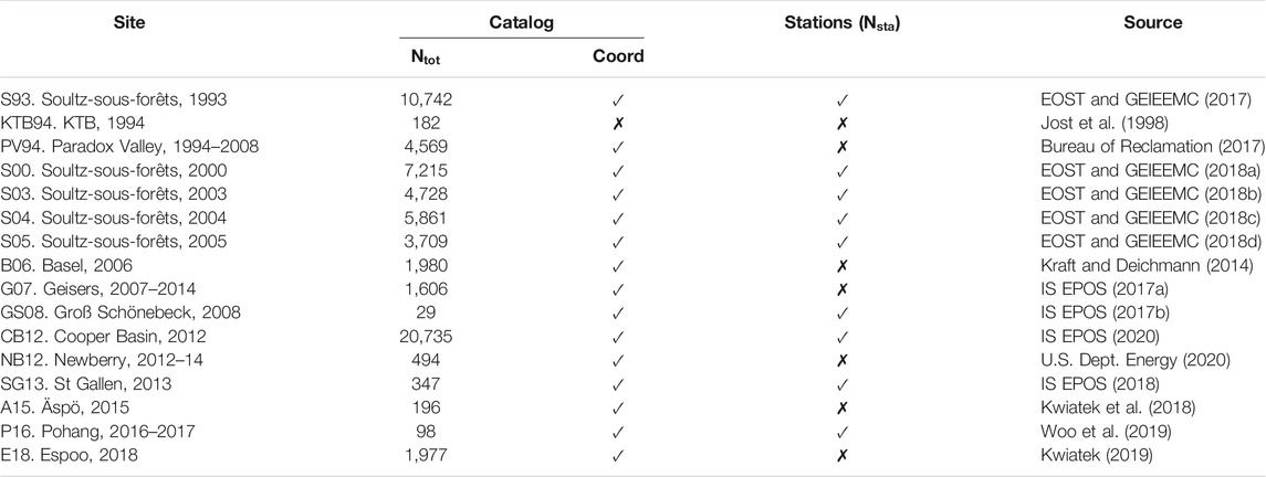
TABLE 1. Available public data for induced seismicity completeness analysis.

Depending on the parameters provided (see Table 1), different completeness analysis levels are achievable. When earthquake coordinates are not included, the study is limited to the bulk MFD analysis (Woessner and Wiemer, 2005; Mignan and Woessner, 2012) and to the application of the Asymmetric Laplace distribution (Mignan, 2019); when earthquake coordinates are included, observed completeness magnitude$m_{c,obs}$ mapping is performed (e.g., Wiemer and Wyss, 2000). In the ideal situation in which the coordinates of the seismic stations are also given, posterior completeness magnitude $m_{c,post}$ maps are also generated using the BMC method (Mignan et al., 2011).

Since this study is solely dedicated to seismicity completeness, data such as total volume injected, flow rate profile, or injection/post-injection windows are not considered (only mentioned in the discussion, Discussion and Perspectives on Data Mining). For statistical analyses related to the fluid injection process at different sites, the reader can refer to, e.g., Dinske and Shapiro (2013), van der Elst et al. (2016), Mignan et al. (2017) or Bentz et al. (2020).

Standard Magnitude Frequency Distribution Analysis

The bulk magnitude frequency distribution (MFD) of an earthquake catalog can be described by a probability density function that takes the form:

$p\left(m\right)=cq\left(m\right)f_{GR}\left(m\right)=cq\left(m\right)e^{-\beta m}$

where $m$ is the earthquake magnitude, $f_{GR}\left(m\right)$ the Gutenberg-Richter law (Gutenberg and Richter, 1944), $q\left(m\right)$ a detection function that controls the shape of the MFD and $c$ a normalization constant so that ${{\displaystyle \int }}^{\text{}}p\left(x\right)dx=1$. The non-cumulative MFD, defined as the number of earthquakes per magnitude bin $m$, is simply $n\left(m\right)=\Delta m{N}_{tot}p\left(m\right)$ with $N_{tot}$ the total number of events and $\Delta m=0.1$ the magnitude bin. The cumulative MFD is more commonly formulated as $N\left(\ge m\right)={10}^{a-bm}$ where $b=\beta /log10$ and $a$ is the overall seismicity activity.

We should have the condition $q\left(\ge m_c\right)=1$ by definition, although it may only tend to 1 if $q$ is unbounded, for example if defined as a cumulative Normal distribution (Ringdal, 1975; Ogata and Katsura, 1993), a log-normal distribution (Martinsson and Jonsson, 2018), or a power-law (so that $p$ can be represented by a gamma distribution; Kijko and Smith, 2017). Mignan (2012), Mignan (2019), in contrast, consider the gradual curvature of the MFD to be due to the sum of "angular" MFDs, each of constant $m_c$, with $q$ a bounded exponential function and $p$ an asymmetric Laplace distribution (see below). "Curved" $q$ functions would then be fitting proxies not representative of the spatially varying and scale-variant detection process (Mignan and Chen, 2016).

Various methods have been proposed to estimate $m_c$ from the bulk MFD, independently of the function $q\left(m\right)$ (see reviews by Woessner and Wiemer, 2005; Mignan and Woessner, 2012). We here consider two non-parametric techniques, the mode of the MFD (also known as "maximum curvature" method; Wiemer and Wyss, 2000) and the Median-Based Analysis of the Segment Slope (MBASS) method (Amorèse, 2007). The $b$-value of the Gutenberg-Richter law can then be estimated with the maximum likelihood estimation (MLE) method (Aki, 1965) for the complete magnitude range $(m_c-\Delta m/2,+\infty )$. It is important to note that $m_c$ values obtained from the bulk MFD can vary significantly across methods, which hampers the evaluation of $b$. A spatial analysis can limit the potential ambiguity (Mignan and Chouliaras, 2014).

Spatial heterogeneities in $m_c$, due at first order to the seismic network spatial configuration (Bayesian Magnitude of Completeness Mapping Method), can be evaluated by a simple mapping procedure. We perform a three-dimensional mapping of $m_{c,obs}(x,y,z)$ in cubic cells 100-m wide. No smoothing kernel (e.g., Wiemer and Wyss, 2000) is used in order to minimize $m_c$ heterogeneities in individual cells. The parameter is estimated by using the mode of the distribution of magnitudes $m$ in each cell $(x,y,z)$. The mode is a reasonable choice for localized data where no significant spatial variations in $m_c$ is expected (Mignan, 2012; Mignan and Chen, 2016). It also yields robust results for sample sizes as low as $n_{min}=4$ earthquakes (Mignan et al., 2011), the threshold used in the present mapping procedure. The set of $m_c$ estimates for all cells is then represented by the vector $m_{c,obs}$, which distribution explains the curvature characteristics of the bulk MFD. Different quantiles of $m_{c,obs}$ can be tested to evaluate $b$. The map of $m_{c,obs}(x,y,z)$ is also used as input for the BMC method described in Bayesian Magnitude of Completeness Mapping Method.

Local MFDs of cells $(x,y,z)$ can be used to estimate both $b$ and the parameter $k$ of the detection function $q$. We consider the asymmetric Laplace probability density function:

$p_{AL}\left(m\right)=\frac{1}{\frac{1}{\kappa -\beta }+\frac{1}{\beta }}\{\begin{array}{cc}{e}^{(\kappa -\beta )(m-m_c)}& , m<m_c\\ e^{-\beta (m-m_c)}& , m\ge m_c\end{array}$

with mode $m_c$ and the detection parameter $k=\kappa /log\left(10\right)$ also estimated using the MLE method (Mignan, 2012; see also equation Asymmetric Laplace Mixture Model). This parameter has been shown to be relatively stable with $k\approx 3$ for natural seismicity in Southern California and Nevada (Mignan, 2012). We apply the same approach to test how this parameter behaves in the context of induced seismicity. We only consider cells with $n_{min}=50$ for those calculations. The asymmetric Laplace distribution is the basic component of the mixture model presented below (Asymmetric Laplace Mixture Model). It also explains why the mode is used to compute $m_c$ in the BMC method (Bayesian Magnitude of Completeness Mapping Method).

Asymmetric Laplace Mixture Model

The sum of local “angular” MFDs of different $m_c$ which forms the bulk "curved" MFD can be approximated by mixture modeling instead of a mapping procedure. This is particularly practical if earthquake coordinates are unavailable with only access to a magnitude vector. The Asymmetric Laplace Mixture Model (ALMM) (Mignan, 2019) is defined as:

$p_{ALMM}\left(m;w_i,m_{c,i},\kappa ,\beta \right)={\displaystyle \sum }_{i=1}^K{w}_i{p}_{AL}(m;m_{c,i},\kappa ,\beta )$

with $K$ the number of Asymmetric Laplace mixture components ordered by $m_c$ value $(m_{c,1}<m_{c,2}<\cdots <m_{c,i}<\cdots <m_{c,K})$ and $w_i$ the mixing weight of the $i$^th component such that ${\displaystyle \sum }_{i=1}^K{w}_i=1$. Parameters $\kappa$ and $\beta$ are assumed constant across components.

Any MFD shape can be fitted by the flexible ALMM based on the Expectation-Maximization (EM) algorithm (Dempster et al., 1977). The initial parameter values are estimated by applying $K$-means (MacQueen, 1967), with $w_i$ the normalized number of events per cluster and $m_{c,i}$ the cluster centroid. Each component is formed of the magnitude vector ${\mathit{M}}_i=(m_1,m_2,\cdots )$. The completeness magnitude $m_{c,i}$ is estimated from the mode of the component. Parameter $\kappa$ is estimated from the incomplete part of the first component ${\mathit{M}}_{left}=\{m\in {\mathit{M}}_1:m\le m_{c,1}-\Delta m/2\}$ while parameter $\beta$ is estimated from the complete part of the last component ${\mathit{M}}_{right}=\{m\in {\mathit{M}}_K:m>m_{c,K}-\Delta m/2\}$. The maximum likelihood estimates are respectively:

$\{\begin{array}{c}\chi =\frac{1}{\left(m_{c,1}-\frac{\text{Δ}m}{2}\right)-{\overline{\mathit{M}}}_{left}}\\ \beta =\frac{1}{{\overline{\mathit{M}}}_{right}-\left(m_{c,K}-\frac{\text{Δ}m}{2}\right)}\end{array}$

with $\chi =\kappa -\beta$ the slope of the incomplete part of the asymmetric Laplace distribution in a log-linear plot.

At each EM iteration $j$, a deterministic version of the expectation step (E-step) attributes a hard label $i$ to each event magnitude from the parameter set ${\theta }_i^{(j-1)}=\{m_{c,i},\kappa ,\beta \}$ defined in the previous iteration $j-1$ ($j=0$ corresponding to the $K$-means estimate). Hard labels are assigned as:

$i=argma{x}_i{p}_{AL}\left(m,{\theta }_i^{(j-1)}\right)$

The maximization step (M-step) then updates the component parameters. The best number of components $K$ is finally selected from the lowest Bayesian Information Criterion estimate $BIC=-LL+1/2(2+K)ln\left(N_{tot}\right)$ (Schwarz, 1978) where $LL$ is the log-likelihood of the ALMM. Details of the full method are given in Mignan (2019). For MFD mixture modeling based on a log-normal component, the reader may refer to Martinsson and Jonsson (2018).

Bayesian Magnitude of Completeness Mapping Method

The last method to be tested in the present study is the Bayesian Magnitude of Completeness (BMC) method that consists in using Bayesian inference to estimate $m_c$ based on incomplete information and prior belief. The incomplete information is the $m_{c,obs}$ map (see Standard Magnitude Frequency Distribution Analysis), which presents gaps in cells of low seismicity and is highly uncertain when estimated from a limited number of earthquake magnitudes. BMC is constrained by a prior model $m_{c,pred}=f\left(d_k\right)$ relating the spatial heterogeneities in $m_c$ to the density of seismic stations, approximated by the distance $d_k$ to the $k$^th nearest station (Mignan et al., 2011). Priors were defined so far in the literature for two-dimensional $m_c$ mapping. We here define a new prior based on three-dimensional distance, which is a requirement for fluid injections characterized by a three-dimensional seismicity cloud centered at the borehole depth and detected by a combination of surface stations and downhole stations. The distance between a cell and a station of coordinates $(x_{sta},y_{sta},z_{sta})$ is thus $d=\sqrt{{(x-x_{sta})}^2+{(y-y_{sta})}^2+{(z-z_{sta})}^2}$. We additionally improve the functional form of the prior, moving from $m_{c,pred}=c_1{d}_k^{c_2}+c_3$ (Mignan et al., 2011) to the form $m_{c,pred}=c_{1}lo{g}_{10}\left(d_k\right)+c_2$, a simpler attenuation function reduced to two free parameters.

Following Bayes' Theorem, we obtain the posterior completeness magnitude $m_{c,post}$ and standard deviation ${\sigma }_{post}$:

$\{\begin{array}{c}{m}_{c,post}=\frac{m_{c,pred}{\sigma }_{obs}^2+m_{c,obs}{\sigma }_{pred}^2}{{\sigma }_{pred}^2+{\sigma }_{obs}^2}\\ {\sigma }_{post}=\sqrt{\frac{{\sigma }_{pred}^2{\sigma }_{obs}^2}{{\sigma }_{pred}^2+{\sigma }_{obs}^2}}\end{array}$

where ${\sigma }_{obs}$ and ${\sigma }_{pred}$ are the standard deviations of $m_c$ observations (based on 100 bootstraps) and of the prior model, respectively. Note that all the aforementioned parameters depend on location $(x,y,z)$, except for ${\sigma }_{pred}$ which is constant.

Results

Results of a Standard ${\mathit{m}}_{\mathit{c}}$ Analysis

We first apply the standard methods of $m_c$ evaluation, based on bulk MFD analysis and $m_c$ mapping. This is the first systematic comparison of completeness level for different induced seismicity sequences.

Figure 1 shows the cumulative bulk MFD for the 16 fluid injections and the matching $m_{c,obs}$ distribution. Figure 1 also shows the estimates $m_{c,mode}$ (dotted vertical line) and $m_{c,MBASS}$ (dashed vertical line) which are often close to the $m_{c,obs}$ median. More conservative estimates of $m_c$, such as the 75% or 90% quantiles of $m_{c,obs}$ seem to provide reasonable $b$-values. We use $q_{90}\left(m_{c,obs}\right)$ to estimate the Gutenberg-Richter slope $b$ in Figure 1. Note that the $m_{c,obs}$ distribution shape matches the curvature of the bulk MFD, which verifies that it is due at first order to spatial heterogeneities. Table 2 lists $m_{c,bulk}$ estimates obtained from different approaches with their respective $b$-values for comparison. For most cases, the $m_c$ range for induced seismicity is comprised between -2 and 1. It goes down to -4 for the Äspö Hard Rock Laboratory experiment where pico-seismicity is detected. Such low $m_c$ values have been reached at other underground laboratories (e.g., Villiger et al., 2020). The range of $b$-values is consistent with the ones obtained by Dinske and Shapiro (2013) for the 5 datasets common to both studies. The authors however only provided one estimate while our Table 2 shows its sensitivity to the minimum magnitude cutoff.

FIGURE 1

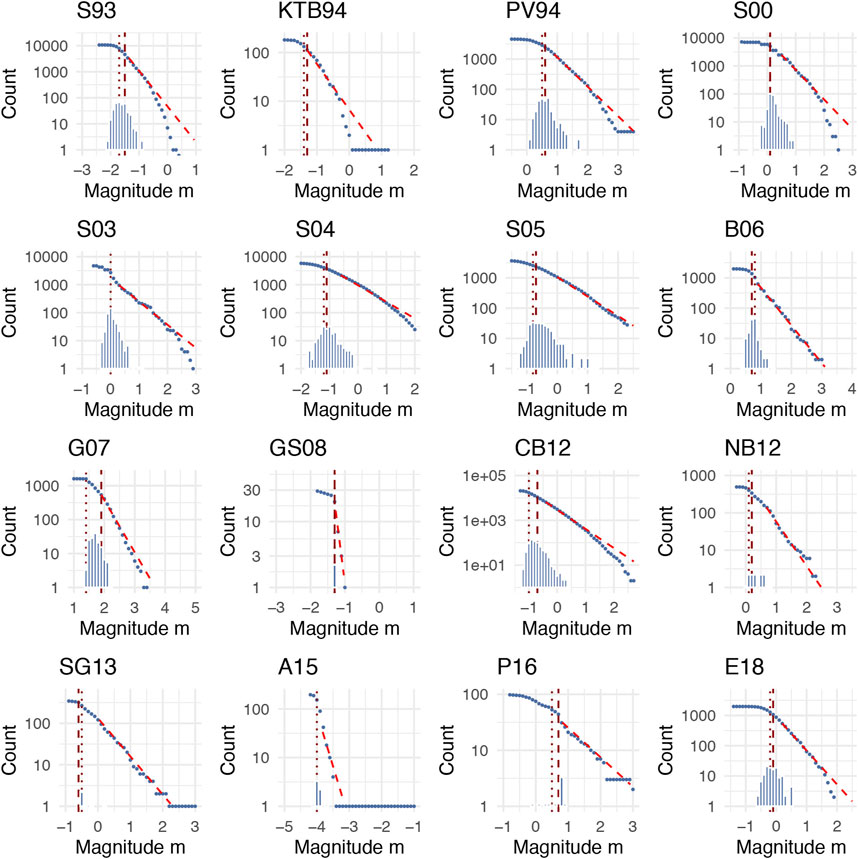
FIGURE 1. Cumulative magnitude frequency distribution (MFD) of 16 underground stimulations. The histogram shows the $m_{c,obs}$ distribution derived from three-dimensional $m_c$ mapping (except for KTB94 for which case coordinates are unavailable). Parameter $b$ (dashed red line) is estimated for $m_c=q_{90}\left(m_{c,obs}\right)$ (for $m_c=m_{c,MBASS}$ in the KTB94 case). The vertical dotted and dashed dark-red lines represent $m_{c,mode}$ and $m_{c,MBASS}$, respectively. See Table 2 for values.

TABLE 2

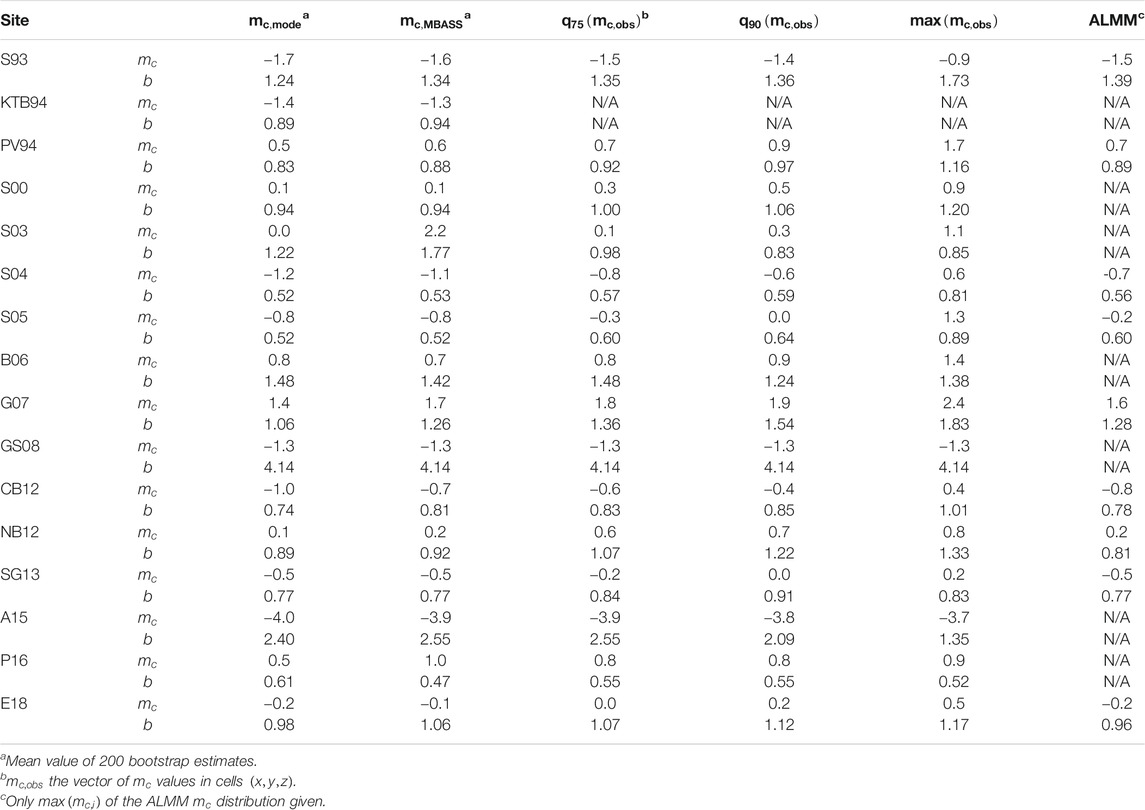
TABLE 2. Parameters $m_c$ and $b\left(m_c\right)$ for different $m_c$ estimation methods applied to the bulk MFD.

Figure 2 shows $m_{c,obs}$ maps at selected depths $z$ for the two stimulations the richest in induced seismicity ($N_{tot}>\mathrm{10,000}$): S93 and CB12. Other maps will be shown in Bayesian Magnitude of Completeness Prior & Posterior m_c Maps when used as input for BMC mapping. Local MFDs for cells that include more than 400 earthquakes are also displayed with their asymmetric Laplace distribution fit. Considering all cells of all sites together, assuming that $k$ and $b$ variations in space are random (Mignan, 2012; Kamer and Hiemer, 2015), we obtain for induced seismicity $k=3.18\pm 1.97$ and $b=1.03\pm 0.48$, which is consistent with natural seismicity regimes but here with significantly larger uncertainties. The plots of Figures 2B,D confirm that the mode of the local MFD is a reasonable choice to estimate $m_c$.

FIGURE 2

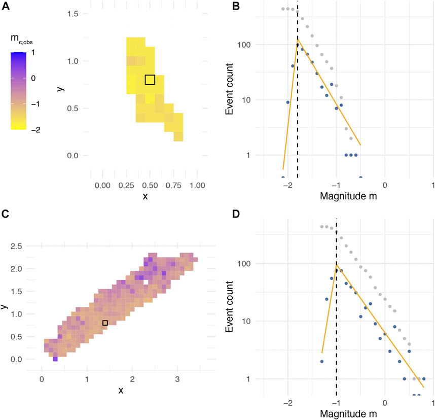
FIGURE 2. Examples of 100 m-resolution $m_{c,obs}$ maps and of local MFDs. (A)$m_{c,obs}$ map at depth $z=-2.7$ km for the 1993 Soultz-sous-Forêts stimulation (S93) (B) local MFD observed in the cell highlighted on the S93 map, with Asymmetric Laplace distribution fit (C)$m_{c,obs}$ map at depth $z=-4.1$ km for the 2012 Cooper Basin stimulation (CB12) (D) local MFD observed in the cell highlighted on the CB12 map, with Asymmetric Laplace distribution fit.

This so-called standard $m_c$ analysis highlights the importance to test several techniques to minimize possible biases in the $b$-value. Mapping remains the best approach to evaluate the $m_c$ range. Reasonable $b$-values are obtained when using conservative $m_{c,obs}$ quantiles (e.g., 75% or 90%).

Asymmetric Laplace Mixture Model Fits

We then apply the ALMM to the 16 magnitude vectors but only get reasonable fits for 9 of them. We find that the ALMM requires $n_{min}>300$ for statistically significant component modeling. It means that the ALMM is not applicable for KTB94, GS08, A15 and P17. It fails for 3 other cases, S00, S03, B06, due to anomalous fluctuations in the observed non-cumulative MFD, which will be discussed in another paragraph.

Figure 3 shows the 9 ALMM fits (for S93, PV94, S04, S05, G07, CB12, NB12, SG13 and E18). Parameters $max\left(m_{c,i}\right)$ and $b$ are listed in Table 2 for comparison with the techniques tested in Results of a Standardm_cAnalysis. Those values range between estimates obtained with the MBASS method and $q_{75}\left(m_{c,obs}\right)$so the method does not seem to provide any new insight into which method to prefer. We observe that the number of$K$ components reflects the gradual curvature of the bulk MFD. For instance, only 2 components suffice to fit the almost angular SG13 MFD while 13 components are needed for the wide S05 MFD, proving the flexibility of the ALMM to fit different MFD shapes. It also verifies that bulk MFDs can be described by the sum of angular MFDs with $m_c$ as modes. We obtain $k=\{7.6,3.3,2.1,2.8,6.5,9.1,4.5,3.7,3.1\}$, respectively, with median 3.7 and mean 4.7.

FIGURE 3

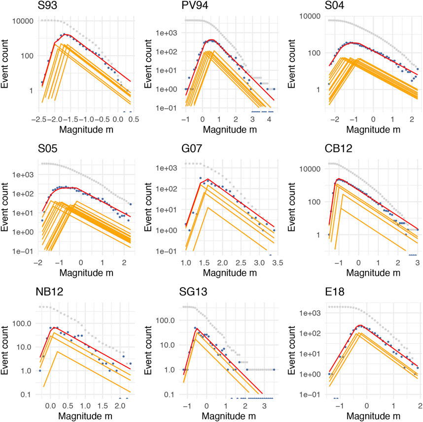
FIGURE 3. Non-cumulative MFD (in blue) of 9 underground stimulations for which an Asymmetric Laplace Mixture Model (ALMM) fit is available, shown in red, with the mixture components shown in orange. See Table 2 for some values.

The ALMM is highly sensible to abnormal fluctuations in the non-cumulative MFD, which are often not visible from the cumulative MFD. In the case of Soultz-sous-Fôrets, the S00 non-cumulative MFD shows significant drops in the number of events inconsistent with any model monotonously increasing up to $m_c$ and monotonously decreasing above $m_c$. In the latter, we observe $n_i=\left\{\mathrm{0,7,7}\right\}$ for bins $m_i=\{0.2, 0.4,0.6\}$; for comparison, $n_i=\left\{\mathrm{1468,1114,717,430}\right\}$ for $m_i=\{0.1, 0.3,0.5,0.7\}$. Such anomaly is smoothed out in the cumulative MFD and does not hamper $b$-value fitting. However, the ALMM anchors at those anomalies, failing to develop into the proper curved MFD. The S03 case shows numerous fluctuations also visible on the cumulative MFD and on the non-trivial evolution of $b$ estimates as the minimum magnitude cutoff increases (Table 2). In regards of the Basel catalog, a zig-zag pattern is observed on the non-cumulative MFD, suggesting an error in rounding between odd and even magnitude digits, which confuses the ALMM algorithm. Those cases indicate more problems with the magnitude vectors than with the ALMM. This suggests that seismologists preparing earthquake catalogs should analyze the non-cumulative distribution of magnitudes to check for potential errors and/or explain the origin of those anomalies incompatible with the Gutenberg-Richter law.

Bayesian Magnitude of Completeness Prior and Posterior ${\mathit{m}}_{\mathit{c}}$ Mmaps

We define a BMC prior model for induced seismicity by combining the relation between $m_c$ and the distance $d_3$ to the 3rd nearest seismic station, observed for the earthquake catalogs that come with seismic network information (Table 1). We choose $d_3$ (over e.g. $d_4$ or $d_5$) since this metric shows the minimal residual error (see ${\sigma }_{pred}$ below). We assume that $m=M_L=M_w$ so that seismicity clouds from different depth levels can be combined to fit one model constrained on a relatively wide $d_3$ range.

Figure 4 represents the BMC prior derived from 7 datasets: S93, S04, S05, GS08, CB12, SG13, and P16. The model, represented by the solid curve, is defined as

$m_{c,pred}=f_{prior}\left(d_3\right)=1.64lo{g}_{10}\left(d_3\right)-1.83; {\sigma }_{pred}=0.37$

with distance $d_3$ in km. Note that the uncertainty ${\sigma }_{pred}$ is greater than the ones obtained from natural seismicity (${\sigma }_{pred}\mathrm{\lesssim }0.25$; e.g., Mignan et al., 2011; Mignan et al., 2013; Kraft et al., 2013; Mignan and Chouliaras, 2014; Tormann et al., 2014). Several reasons may be advanced: different sites are here combined, representative of different soil conditions and thus potentially of different seismic attenuation functions; considering the depth component may add uncertainty on distance measures; finally, the model is constrained on far shorter distance ($d_3<10$ km) compared to up to hundreds of kilometers in regional catalogs. It is interesting to compare the model prediction to the pico-seismicity completeness level $m_c\approx -4$ observed at Äspö (A15). We learn from Kwiatek et al. (2018) that sensors were located between a few meters and 100 m from the injection borehole. We independently predict $m_{c,pred}\left(10m\right)=-5.1$ and $m_{c,pred}\left(100m\right)=-3.5$, which is a reasonable approximation. Adding further datasets to the model will help better constraining it.

FIGURE 4

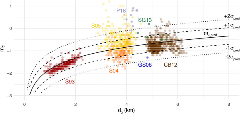
FIGURE 4. Prior model $m_{c,pred}=f\left(d_3\right)$ of the Bayesian Magnitude of Completeness (BMC) method for the three-dimensional induced seismicity case with distance $d_3$ to the third nearest seismic station.

Two datasets, S00 and S03, were not included in this analysis as event declaration depended in those cases on two triggering conditions from both the downhole and surface networks (EOST and GEIEEMC, 2018a; EOST and GEIEEMC, 2018b), which is likely inconsistent with the simple $d_3$ metric. Testing with $d_3$ leads to a systematic bias requiring a correction $f_{prior}\left(d_3\right)+1$. Use of such formula would however be inadequate. It remains unclear if the magnitude scale used for S00 and S03, duration magnitude $m_D$, could also play a role in the observed $m_c$ shift upward.

We then combine the $m_{c,obs}$ with the prior model to derive the posterior $m_{c,post}$ maps. We show some examples taken from S93 and CB12 in Figure 5. The BMC methods fills all the gaps in $m_{c,obs}$, and provides completeness levels expected for future seismicity, e.g., during cloud development as more fluids get injected, which can be of use to the injection operators. The BMC method also decreases $m_c$ uncertainties, as can be observed when comparing ${\sigma }_{post}$ to ${\sigma }_{obs}$. Note finally that the BMC method is consistent with the Asymmetric Laplace detection model previously described. It makes use of the mode of local MFDs so that the number of cells with $m_{c,obs}$ values is maximized while $f_{prior}$ explains how $m_c$ evolves in space, from which the bulk FMD, approximated by the ALMM, emerges.

FIGURE 5

FIGURE 5. Observed $m_{c,obs}$ vs. posterior $m_{c,post}$ maps derived from the BMC prior model. (A) S93 at depth $z=-3.1$ km (B) CB12 at depth $z=-4.2$ km.

Discussion and Perspectives on Data Mining

We reviewed some standard approaches to estimate the completeness magnitude $m_c$ and ported the recent ALMM mixture and BMC mapping methods to the induced seismicity context. We provided various estimates of $m_c$, $b$ (Table 2) and detection parameter $k$ so that better informed choices could be made in future statistical analyses of induced seismicity. We observed that the $k$-value for induced seismicity is compatible with the one obtained for natural seismicity, suggesting a common detection process although uncertainties are high. We also provided the first parameterization of the BMC prior for three-dimensional seismicity clouds.

The present study could help refine future seismic hazard analyses, since the parameter $m_c$ is a prerequisite to the estimation of the hazard inputs: the $a$- and $b$-values of the Gutenberg-Richter law. In contrast to the tectonic regime, the $a$-value is normalized to the total injected volume $V$ for comparisons across stimulations, so that $N(\ge m)=V{10}^{a_{fb}-bm}$ with $a_{fb}$ the normalized $a$-value, called underground feedback parameter in Mignan et al. (2017) and seismogenic index in poroelasticity parlance (e.g., Dinske and Shapiro, 2013). The term $a_{fb}$ is agnostic, while alternatives to poroelasticity exist (e.g., Mignan, 2016). A priori knowledge of the Gutenberg-Richter parameters is required in pre-stimulation risk assessment (e.g., Mignan et al., 2015; Broccardo et al., 2020), and the parameterization may be updated during stimulations via a dynamic traffic light system (e.g., Broccardo et al., 2017; Mignan et al., 2017). Note also that the maximum magnitude $m_{mas}$ relates directly to $b$ (e.g., van der Elst et al., 2016; Broccardo et al., 2017).

We first showed the impact of $m_c$ values on $b$ and selected $q_{90}\left(m_{c,obs}\right)$ as conservative estimates. We also found that the ALMM does not provide any new insight to the problem and is hampered by fluctuations in the non-cumulative MFD observed in some experiments. As a consequence, $m_c$ mapping remains the best alternative and is simple enough to implement.

While $m_c$ also alters $a_{fb}$ via $b$, we can consider another aspect that may improve our knowledge of the underground feedback. It has been observed that $a_{fb}$ significantly varies across sites and across stimulations at a same site (e.g., Dinske and Shapiro, 2013; Mignan et al., 2017) which may lead to risk aversion of potential investors in geo-energy for instance (Mignan et al., 2019). One may difficultly infer $a_{fb}$ from the literature when no information about completeness is given, which is especially true for early articles. However, we can now estimate $a_{fb}$ despite the total number of events induced $N(\ge m_{?})$ being potentially ambiguous. To illustrate the problem posed, let us consider the 1988 stimulation at Hijiori, Japan. We learn from Sasaki (1998) that $N(\ge m_{?})=65$ micro-earthquakes were observed above $m_{?}=-4$ (their Figure 6) for an injected volume $V=\mathrm{2,000}$ m³. The equation $a_{fb}=lo{g}_{10}(N(\ge m_{?})/V)+b{m}_{?}$ is valid only if $m_{?}\ge m_c$. Information in Sasaki (1998) is however ambiguous, and we may have $m_{?}=min\left(m\right)<m_c$ instead, which would underestimate the underground feedback activation since the data would then be incomplete. Considering all datasets of Table 1 with $N_{tot}>200$, we can estimate from their censored data the metrics $\delta m=m_c-min\left(m\right)$ and $\gamma =N(\ge m_c)/N(\ge min\left(m\right))$ which range on the intervals $[0.8,1.9]$ and $[0.20,0.37]$, respectively (with no trend observed). The distributions are shown in Figure 6A alongside the corrected underground feedback parameter $a_{fb,corrected}=lo{g}_{10}(\gamma N(\ge min\left(m\right))/V)+b(min\left(m\right)+\delta m)$. Assuming $\delta m$ and $\gamma$ representative (and $b=1$, see Results of a Standardm_cAnalysis), the 1988 Hijiori underground feedback activation may be $a_{fb,correct}=-5.5$ if $m_{?}=m_c$, or $a_{fb,corrected}=[-5.4,-3.9]$ if $m_{?}=min\left(m\right)$. Despite the ambiguity, an estimate may therefore still be provided. A review of the literature could provide additional values from other fluid injections to better constrain the range of $a_{fb}$ to be considered as a priori information in risk assessment, which is so far potentially biased toward high $a_{fb}$ values (e.g., Mignan et al., 2017).

FIGURE 6

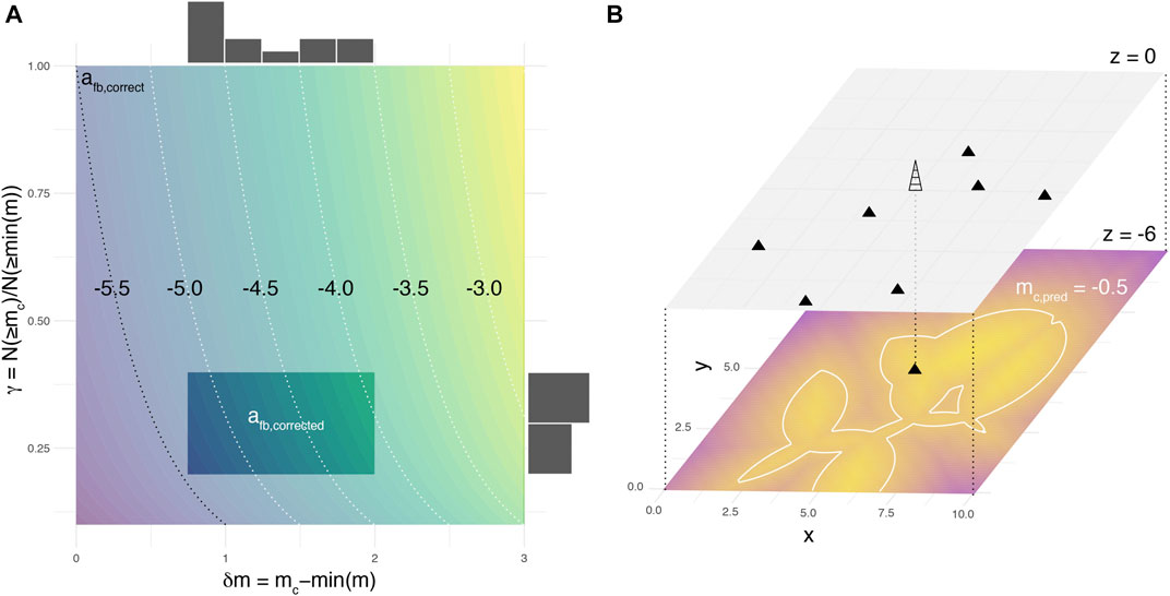
FIGURE 6. Induced seismicity data mining potential from completeness analysis. (A) Estimating the underground feedback parameter $a_{fb}$ despite potential ambiguity on the minimum magnitude cutoff mentioned in the literature, by using information on $\delta m=m_c-min\left(m\right)$ and $\gamma =N(\ge m_c)/N(\ge min\left(m\right))$ obtained for the sites considered in the present study (histograms) – $a_{fb}$ estimates given for $b=1$, $N(\ge m_{?})=65$ and $V=\mathrm{2,000}$ m³ (1988 Hijiori case) (B) Predicting the completeness level of a planned seismic network configuration using the prior model $f_{prior}\left(d_3\right)$ of the BMC method (here with 8 stations, 7 randomly distributed at the surface and 1 located at the ad-hoc borehole with coordinates $(\mathrm{5,5},-6)$ km).

Finally, if the BMC method allows defining robust $m_c$ maps (no spatial gap, uncertainty constrained by the seismic network configuration), BMC may be even more useful for seismic network planification (e.g., Kraft et al., 2013) prior to new stimulations. Seismic safety criteria can be mapped into magnitude thresholds not to be crossed (Mignan et al., 2017), which tell us the completeness magnitude level required for sound statistical analysis. One can then use the BMC prior $f_{prior}\left(d_3\right)$ to test how a completeness level can be achieved given a seismic network configuration. Figure 6B illustrates such an application. The two approaches presented in Figure 6 demonstrate how induced seismicity data mining can be done from completeness magnitude knowledge, which in turn can improve induced seismicity monitoring, modeling and managing.

Data Availability Statement

Publicly available datasets were analyzed in this study. This data can be found here See Table 1 and reference list.

Author Contributions

AM did all the research and writing.

Conflict of Interest

The author declares that the research was conducted in the absence of any commercial or financial relationships that could be construed as a potential conflict of interest.

Footnotes

¹

Vásquez, R., and Bravo de Guenni, L. n. d. Bayesian estimation of the spatial variation of the completeness magnitude for the Venezuelan seismic catalogue. Available at: https://www.statistics.gov.hk/wsc/CPS204-P47-S.pdf. (Accessed Aug 2014)

References

Ake, J., Mahrer, K., O’Connell, D., and Block, L. (2005). Deep-injection and closely monitored induced seismicity at Paradox Valley, Colorado. Bull. Seismol. Soc. Am. 95, 664–683. doi:10.1785/0120040072

CrossRef Full Text | Google Scholar

Aki, K. (1965). Maximum likelihood estimate of b in the formula Log N = a-bM and its confidence limits. Bull. Earthq. Res. Inst. Univ. Tokyo 43, 237–239.

Google Scholar

Amorèse, D. (2007). Applying a change-point detection method on frequency-magnitude distributions. Bull. Seismol. Soc. Am. 97 (1), 742–751. doi:10.1785/0120060181

CrossRef Full Text | Google Scholar

Baisch, S., Rothert, E., Stang, H., Vörös, R., Koch, C., and McMahon, A. (2015). Continued geothermal reservoir stimulation experiments in the Cooper Basin (Australia). Bull. Seismol. Soc. Am. 105, 198–209. doi:10.1785/0120140208

CrossRef Full Text | Google Scholar

Bentz, S., Kwiatek, G., Martínez-Garzón, P., Bohnhoff, M., and Dresen, G. (2020). Seismic moment evolution during hydraulic stimulations. Geophys. Res. Lett. 47, e2019GL086185. doi:10.1029/2019gl086185

CrossRef Full Text | Google Scholar

Brandt, M. B. C. (2019). Performance of the South African national seismograph network from october 2012 to february 2017: spatially varying magnitude completeness. S. Afr. J. Geol. 122, 57–68. doi:10.25131/sajg.122.0004

CrossRef Full Text | Google Scholar

Broccardo, M., Mignan, A., Grigoli, F., Karvounis, D., and Rinaldi, A. P (2020). Induced seismicity risk analysis of the hydraulic stimulation of a geothermal well on Geldinganes, Iceland. Nat. Hazards Earth Syst. Sci. 20 (1573-1), 593. doi:10.5194/nhess-20-1573-2020

CrossRef Full Text | Google Scholar

Broccardo, M., Mignan, A., Wiemer, S., Stojadinovic, B., and Giardini, D. (2017). Hierarchical bayesian modeling of fluid-induced seismicity. Geophys. Res. Lett. 44 (11), 357–411. doi:10.1002/2017gl075251

CrossRef Full Text | Google Scholar

Bureau of Reclamation (2017). Paradox Valley earthquake catalogue. Available at: https://www.usbr.gov/uc/wcao/progact/paradox/RI.html. (Accessed June 2017)

Calò, M., and Dorbath, C. (2013). Different behaviours of the seismic velocity field at Soultz-sous-Fôrets revealed by 4-D seismic tomography: case study of GPK3 and GPK2 injection tests. Geophys. J. Int. 194 (1), 119–121. doi:10.1093/gji/ggt153

CrossRef Full Text | Google Scholar

Charléty, J., Cuenot, N., Dorbath, L., Dorbath, C., Haessler, H., and Frogneux, M. (2007). Large earthquakes during hydraulic stimulations at the geothermal site of Soultz-sous-Forêts. Int. J. Rock Mech. Mining Sci. 44 (1), 105–111. doi:10.1016/j.ijrmms.2007.06.003

CrossRef Full Text | Google Scholar

Cladouhos, T. T., Petty, S., Nordin, Y., Moore, M., Grasso, K., and Uddenberg, M. (2013). “Microseismic monitoring of Newberry Volcano EGS demonstration,” in Proc. 38th workshop geotherm. Reservoir. Engineering, February 11-13, 2013 (Stanford, CA: Stanford University).

Google Scholar

Cladouhos, T. T., Petty, S., Swyer, M., Uddenberg, M., and Nordin, Y. (2015). “Results from Newberry Volcano EGS demonstration,” in Proc. 40th workshop geotherm. Reserv. Eng, January 26–28, 2015 (Stanford, CA: Stanford University).

CrossRef Full Text | Google Scholar

Cornet, F. H., Helm, J., Poitrenaud, H., and Etchecopar, A. (1997). Seismic and aseismic slips induced by large-scale fluid injections. Pure Appl. Geophys. 150, 563–583. doi:10.1007/s000240050093

CrossRef Full Text | Google Scholar

Cuenot, N., Dorbath, C., and Dorbath, L. (2008). Analysis of the microseismicity induced by fluid injections at the EGS site of soultz-sous-forêts (alsace, France): implications for the characterization of the geothermal reservoir properties. Pure Appl. Geophys. 165, 797–828. doi:10.1007/s00024-008-0335-7

CrossRef Full Text | Google Scholar

Dempster, A. P., Laird, N. M., and Rubin, D. B. (1977). Maximum likelihood from incomplete data via theEMAlgorithm. J. R. Stat. Soc. Ser. B 39, 1–22. doi:10.1111/j.2517-6161.1977.tb01600.x

CrossRef Full Text | Google Scholar

Diehl, T., Kraft, T., Kissling, E., and Wiemer, S. (2017). The induced earthquake sequence related to the St. Gallen deep geothermal project (Switzerland): fault reactivation and fluid interactions imaged by microseismicity. J. Geophys. Res. Solid Earth 122 (7), 272–277. doi:10.1002/2017jb014473

CrossRef Full Text | Google Scholar

Dinske, C., and Shapiro, S. A. (2013). Seismotectonic state of reservoirs inferred from magnitude distributions of fluid-induced seismicity. J. Seismol. 17, 13–25. doi:10.1007/s10950-012-9292-9

CrossRef Full Text | Google Scholar

EOST and GEIEEMS (2017). Episode: 1993 stimulation soultz-sous-forêts [collection]. EOST CDGP 107, 2247–2257. doi:10.25566/SSFS1993

CrossRef Full Text | Google Scholar

EOST and GEIEEMS (2018a). Episode: 2000 stimulation soultz-sous-forêts [collection]. EOST CDGP [Epub ahead of print]. doi:10.25577/SSFS2000

CrossRef Full Text | Google Scholar

EOST and GEIEEMS (2018b). Episode: 2003 stimulation soultz-sous-forêts [collection]. EOST CDGP [Epub ahead of print]. doi:10.25577/SSFS2003

CrossRef Full Text | Google Scholar

EOST and GEIEEMS (2018c). Episode: 2004 stimulation soultz-sous-forêts [collection]. EOST CDGP [Epub ahead of print]. doi:10.25577/SSFS2004

CrossRef Full Text | Google Scholar

EOST and GEIEEMS (2018d). Episode: 2005 stimulation soultz-sous-forêts [collection]. EOST CDGP [Epub ahead of print]. doi:10.25577/SSFS2005

CrossRef Full Text | Google Scholar

Gutenberg, B., and Richter, C. F. (1944). Frequency of earthquakes in California. Bull. Seismol. Soc. Am. 34, 184–188.

Google Scholar

Häring, M. O., Schanz, U., Ladner, F., and Dyer, B. C. (2008). Characterisation of the Basel 1 enhanced geothermal system. Geothermics 37, 469–495. doi:10.1016/j.geothermics.2008.06.002

CrossRef Full Text | Google Scholar

IS EPOS (2017a). Episode: THE geysers Prati 9 and Prati 29 cluster. Available at: https://tcs.ah-epos.eu/#episode. (Accessed November 2020)

Google Scholar

IS EPOS (2017b). Episode: gross schoenebeck. Available at: https://tcs.ah-epos.eu/#episode. (Accessed November 2020)

Google Scholar

IS EPOS (2018). Episode THE GEYSERS Prati 9 and Prati 29 cluster. Available at: https://tcs.ah-epos.eu/#episode. (Accessed November 2020)

Google Scholar

IS EPOS (2020). Episode: cooper BASIN. Available at: https://tcs.ah-epos.eu/#episode. (Accessed November 2020)

Google Scholar

Jost, M. L., Büsselberg, T., Jost, Ö., and Harjes, H. P. (1998). Source parameters of injection-induced microearthquakes at 9 km depth at the KTB deep drilling site, Germany. Bull. Seismol. Soc. Am. 88, 815–832.

Google Scholar

Kamer, Y., and Hiemer, S. (2015). Data-driven spatial b value estimation with applications to California seismicity: to b or not to b. J. Geophys. Res. Solid Earth 120 (5), 191–195. doi:10.1002/2014jb011510

CrossRef Full Text | Google Scholar

Kijko, A., and Smit, A. (2017). Estimation of the frequency-magnitude gutenberg-richterb‐value without making assumptions on levels of completeness. Seismol. Res. Lett. 88, 311–318. doi:10.1785/0220160177

CrossRef Full Text | Google Scholar

Kraft, T., and Deichmann, N. (2014). High-precision relocation and focal mechanism of the injection-induced seismicity at the Basel EGS. Geothermics 52, 59–73. doi:10.1016/j.geothermics.2014.05.014

CrossRef Full Text | Google Scholar

Kraft, T., Mignan, A., and Giardini, D. (2013). Optimization of a large-scale microseismic monitoring network in northern Switzerland. Geophys. J. Int. 195, 474–490. doi:10.1093/gji/ggt225

CrossRef Full Text | Google Scholar

Kwiatek, G., Bohnhoff, M., Dresen, G., Schulze, A., Schulte, T., and Zimmermann, G. (2010). Microseismicity induced during fluid-injection: a case study from the geothermal site at Groß Schönebeck, North German Basin. Acta Geophys. 58, 995–1020. doi:10.2478/s11600-010-0032-7

CrossRef Full Text | Google Scholar

Kwiatek, G. (2019). Controlling fluid-induced seismicity during a 6.1-km-deep geothermal stimulation in Finland. Sci. Adv. 5, eaav7224. doi:10.1126/sciadv.aav7224

PubMed Abstract | CrossRef Full Text | Google Scholar

Kwiatek, G., Martínez-Garzón, P., Dresen, G., Bohnhoff, M., Sone, H., and Hartline, C. (2015). Effects of long-term fluid injection on induced seismicity parameters and maximum magnitude in northwestern part of the Geysers geothermal field. J. Geophys. Res. Solid Earth 120 (7), 101–107. doi:10.1002/2015jb012362

CrossRef Full Text | Google Scholar

Kwiatek, G., Martínez-Garzón, P., Plenkers, K., Leonhardt, M., Zang, A., and von Specht, S. (2018). Insights into complex subdecimeter fracturing processes occurring during a water injection experiment at depth in Äspö Hard Rock Laboratory, Sweden. J. Geophys. Res. Solid Earth 123, 6616–6635. doi:10.1029/2017JB014715

CrossRef Full Text | Google Scholar

MacQueen, J. (1967). “Some methods for classification and analysis of multivariate observations,” in Proc. 5th berkeley symposium on mathematics, statistics and probability Editors M. L. M. Le Cam and J. Neyman (Univ. California Press), vol. 5.1, 281–297.

Google Scholar

Martinsson, J., and Jonsson, A. (2018). A new model for the distribution of observable earthquake magnitudes and applications to $b$ -value estimation. IEEE Geosci. Rem. Sens. Lett. 15, 833–837. doi:10.1109/lgrs.2018.2812770

CrossRef Full Text | Google Scholar

Mignan, A., Broccardo, M., Wiemer, S., and Giardini, D. (2017). Induced seismicity closed-form traffic light system for actuarial decision-making during deep fluid injections. Sci. Rep. 7, 13607. doi:10.1038/s41598-017-13585-9

PubMed Abstract | CrossRef Full Text | Google Scholar

Mignan, A., and Chen, C.-C. (2016). The spatial scale of detected seismicity. Pure Appl. Geophys. 173, 117–124. doi:10.1007/s00024-015-1133-7

CrossRef Full Text | Google Scholar

Mignan, A., and Chouliaras, G. (2014). Fifty years of seismic network performance in Greece (1964-2013): spatiotemporal evolution of the completeness magnitude. Seismol. Res. Lett. 85, 657–667. doi:10.1785/0220130209

CrossRef Full Text | Google Scholar

Mignan, A. (2012). Functional shape of the earthquake frequency-magnitude distribution and completeness magnitude. J. Geophys. Res. 117, B08302. doi:10.1029/2012jb009347

CrossRef Full Text | Google Scholar

Mignan, A. (2019). Generalized earthquake frequency-magnitude distribution described by asymmetric Laplace mixture modelling. Geophys. J. Int. 219 (1), 348–351. doi:10.1093/gji/ggz373

CrossRef Full Text | Google Scholar

Mignan, A., Jiang, C., Zechar, J. D., Wiemer, S., Wu, Z., and Huang, Z. (2013). Completeness of the Mainland China earthquake catalog and implications for the setup of the China earthquake forecast testing center. Bull. Seismol. Soc. Am. 103, 845–859. doi:10.1785/0120120052

CrossRef Full Text | Google Scholar

Mignan, A., Landtwing, D., Kästli, P., Mena, B., and Wiemer, S. (2015). Induced seismicity risk analysis of the 2006 Basel, Switzerland, Enhanced Geothermal System project: influence of uncertainties on risk mitigation. Geothermics 53, 133–146. doi:10.1016/j.geothermics.2014.05.007

CrossRef Full Text | Google Scholar

Mignan, A., Karvounis, D., Broccardo, M., Wiemer, S., and Giardini, D. (2019). Including seismic risk mitigation measures into the Levelized Cost of Electricity in enhanced geothermal systems for optimal siting. Appl. Energ. 238, 831–850. doi:10.1016/j.apenergy.2019.01.109

CrossRef Full Text | Google Scholar

Mignan, A. (2016). Static behaviour of induced seismicity. Nonlin. Process. Geophys. 23, 107–113. doi:10.5194/npg-23-107-2016

CrossRef Full Text | Google Scholar

Mignan, A., Werner, M. J., Wiemer, S., Chen, C. C., and Wu, Y. M. (2011). Bayesian estimation of the spatially varying completeness magnitude of earthquake catalogs. Bull. Seismol. Soc. Am. 101, 1371–1385. doi:10.1785/0120100223

CrossRef Full Text | Google Scholar

Mignan, A., and Woessner, J. (2012). Estimating the magnitude of completeness for earthquake catalogs. Available at: http://www.corssa.org: Community Online Resource for Statistical Seismicity Analysis. (Accessed November 2020)

Google Scholar

Ogata, Y., and Katsura, K. (1993). Analysis of temporal and spatial heterogeneity of magnitude frequency distribution inferred from earthquake catalogues. Geophys. J. Int. 113, 727–738. doi:10.1111/j.1365-246x.1993.tb04663.x

CrossRef Full Text | Google Scholar

Panzera, F., Mignan, A., and Vogfjörð, K. S. (2017). Spatiotemporal evolution of the completeness magnitude of the Icelandic earthquake catalogue from 1991 to 2013. J. Seismol. 21, 615–630. doi:10.1007/s10950-016-9623-3

CrossRef Full Text | Google Scholar

Ringdal, F. (1975). On the estimation of seismic detection thresholds. Bull. Seismol. Soc. Am. 65 (1), 631.

Google Scholar

Sasaki, S. (1998). Characteristics of microseismic events induced during hydraulic fracturing experiments at the Hijiori hot dry rock geothermal energy site, Yamagata, Japan. Tectonophysics 289, 171–188. doi:10.1016/s0040-1951(97)00314-4

CrossRef Full Text | Google Scholar

Tormann, T., Wiemer, S., and Mignan, A. (2014). Systematic survey of high-resolution b value imaging along Californian faults: inference on asperities. J. Geophys. Res. Solid Earth 119 (2), 029–32. doi:10.1002/2013jb010867

CrossRef Full Text | Google Scholar

U.S. Department of Energy (2020). Newberry. Available at: http://fracture.lbl.gov/cgi-bin/Web_CatalogSearch.py. (Accessed November 2020)

Google Scholar

van der Elst, N. J., Page, M. T., Weiser, D. A., Goebel, T. H. W., and Hosseini, S. M. (2016). Induced earthquake magnitudes are as large as (statistically) expected. J. Geophys. Res. Solid Earth 121 (4), 575–584. doi:10.1002/2016jb012818

CrossRef Full Text | Google Scholar

Villiger, L., Gischig, V. S., Doetsch, J., Krietsch, H., and Dutler, N. O. (2020). Influence of reservoir geology on seismic response during decameter-scale hydraulic stimulations in crystalline rock. Solid Earth 11, 627–655. doi:10.5194/se-11-627-2020

CrossRef Full Text | Google Scholar

Vorobieva, I., Narteau, C., Shebalin, P., Beauducel, F., Nercessian, A., and Clouard, V. (2013). Multiscale mapping of completeness magnitude of earthquake catalogs. Bull. Seismol. Soc. Am. 103 (2), 188–192. doi:10.1785/0120120132

CrossRef Full Text | Google Scholar

Wiemer, S., and Wyss, M. (2000). Minimum magnitude of completeness in earthquake catalogs: examples from Alaska, the western United States, and Japan. Bull. Seismol. Soc. Am. 90, 859–869. doi:10.1785/0119990114

CrossRef Full Text | Google Scholar

Woessner, J., and Wiemer, S. (2005). Assessing the quality of earthquake catalogues: estimating the magnitude of completeness and its uncertainty. Bull. Seismol. Soc. Am. 95, 684–698. doi:10.1785/0120040007

CrossRef Full Text | Google Scholar

Woo, J.-U., Kim, M., Sheen, D.-H., Kang, T.-S., Rhie, J., and Grigoli, F. (2019). An in-depth seismological analysis revealing a causal link between the 2017 M_w 5.5 Pohang earthquake and EGS project. J. Geophys. Res. Solid Earth 124 (13), 060–113. doi:10.1029/2019jb018368

CrossRef Full Text | Google Scholar