Broadband Q-Factor Imaging for Geofluid Detection in the Gulf of Trieste (Northern Adriatic Sea)

Seismic surveys allow estimating lithological parameters, as P-wave velocity and anelastic absorption, which can detect the presence of fracture and fluids in the geological formations. Recently, a new method has been proposed for high-resolution imaging of anelastic absorption, which combines a macro-model from seismic tomography with a micro-model obtained by the pre-stack depth migration of a seismic attribute, i.e., the instantaneous frequency. As a result, we can get a broadband image that provides clues about the presence of saturating fluids. When the saturation changes sharply, as for gas reservoirs with an impermeable caprock, the acoustic impedance contrast produces “bright spots” because of the resulting high reflectivity at its top. When the fluid content changes smoothly, the anelastic absorption becomes a good detector, as fluid-filled formations absorb more seismic energy than hard rocks. We apply this method for imaging the anelastic absorption in a regional seismic survey acquired by OGS in the Gulf of Trieste (northern Adriatic Sea, Italy).

Introduction

In the Adriatic Sea, the occurrence of fluids within the sediment and fluid seeps at the sea floor are well known. Source of these fluids have been identified in the buried several kilometer thick Meso-Cenozoic carbonate reservoir, with salty water occurrence (Cimolino et al., 2010), and within the overlying Late Cenozoic terrigenous sedimentary units bearing biogenic gas (e.g., Casero, 2004). Fluids upward migration from several km deep rocks and feeding local seeps have been documented in the central and northern Adriatic (Geletti et al., 2008; Busetti et al., 2013; Donda et al., 2019). Fluid accumulation in the shallow sediments and fluid seeps have been encountered by the high-resolution seismic, often associated to fluid seeps, in the Adriatic basin (e.g., Hovland and Curzi, 1989; Conti et al., 2002), including the Gulf of Trieste (e.g., Gordini et al., 2004; Busetti et al., 2020).

Fluid accumulation in the shallow sediments and fluid seeps are expected to be encountered by the high-resolution seismic profile acquired in the Gulf of Trieste in 2009 by OGS (Figure 1). The aim of this paper is characterizing some shallow formations by a broadband Q-factor imaging, as a low Q factor is often associated to rocks saturation and unconsolidated formations. This method merges the macro-model obtained from Q tomography with the micro-model provided by the pre-stack depth migration of the instantaneous frequency. In this way, also tiny local anomalies might be detected, pushing the resolution of seismic data up to its physical limits.

FIGURE 1

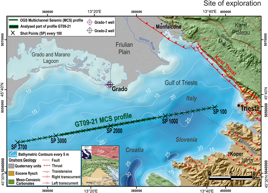
FIGURE 1. Location map of the seismic profile GT09–21 (green line) with shot points (SP) every 100 (black crosses) acquired by OGS in the Gulf of Trieste (Adriatic Sea). Circles show position of Grado geothermal wells. Bathymetry in depth with cells of 50 m, gridding performed by Zampa (2020) by using grids from Italy and Slovenia (Trobec et al., 2018) and Croatia (EMODnet Digital Bathymetry, 2018). Onshore geology is represented for Friulian Plain and Italian Karst Plateau (Cucchi et al., 2013), Slovenian Karst Plateau (Jurkovšek et al., 2016) and Istria (Placer et al., 2010). Digital Elevation Model compiled for Italy (10 m cells; IRDAT-FVG, 2017), Slovenia (10 m cells; Arso, 2017) and Istria (25 m cells; EU-DEM, 2017). Inset: chains and foreland domains of the region surrounding the Gulf of Trieste. Map compiled by using ArcGis® software by Esri; datum WGS84, projection UTM33.

Delineating areas where the fracture density is higher provides relevant hints for geodynamic and geothermal studies. They highlight faulted or stressed formations, whose response to seismic surveys affects two propagation phenomena: anisotropy and anelastic absorption (see, e.g., Shapiro and Hubral 1999; Carcione 2014; Song et al., 2020b, among others). Anisotropy measurement requires very expensive acquisition technologies, as full-azimuth 3D surveys, possibly using ocean-bottom seismometers. Detecting anelastic absorption is more affordable, although it may be anisotropic itself: 2D surveys can provide reasonable estimations at cheaper costs.

The anelastic absorption we observe is actually a composite effect of other causes too, as fluid saturation, pore pressure, random distribution of inhomogeneities and frequency tuning by thin layers, in addition to fractures. Thus, it is not a direct indicator of fluids’ presence, unless there is a borehole calibration or geological information that may single out one or part of these possible contributions (Jannsen et al., 1985; Tonn 1991). Trying to distinguish them is still an open challenge and a subject for current research (Wu 1985; Best et al., 1994; Hackert and Parra 2003; Helle et al., 2003; Picotti and Carcione 2006; Mulder and Hak 2009; Cheng and Margrave 2012; Ba et al., 2015; Bai et al., 2017; Agudo et al., 2018; Song et al., 2020a, among others). In this paper, we apply a recent method introduced by Lin et al. (2018) to marine seismic data, producing high-resolution, broadband images of the anelastic absorption contrasts, and the related Q factor. These parameters allow characterizing the geological formations and provide better clues about the fluids’ pathways.

Geological Setting

The Gulf of Trieste is a shallow marine area located in the north-easternmost corner of the Adriatic Sea (Figure 1). The geological setting is characterized by several kilometer-thick carbonate units, deposited from Permian to Early Cenozoic (Busetti et al., 2010). During the Cretaceous, the carbonate sedimentation formed the aggradation of about 1 km thick Friuli and Dinaric Carbonate Platform, with the shelf margin located in the western side of the Gulf of Trieste, outcropping along the eastern coast and at the north-west of the Istria peninsula. At the same time, in the western basin area, pelagic carbonate draped the basin floor. The carbonate sedimentation ended with the compressional phase of the Dinaric mountain chain, which caused the development of the Dinaric foredeep, with the eastern tilted carbonate platform. The Dinaric foredeep was filled by the turbiditic sequence of Eocene, produced by the progressive erosion of the rising mountains, outcropping along the eastern and southern coasts of the gulf (Figure 2). In the same period, the basin was progressively filled by the Gallare Marls and topped by the Early Miocene Cavanella Group, composed of sand, sandstone and marls. These lithologies were shaped by the main erosional event occurred at the Miocene end, due to the Messinian Salinity Crisis of the Mediterranean Sea (Busetti et al., 2010).

FIGURE 2

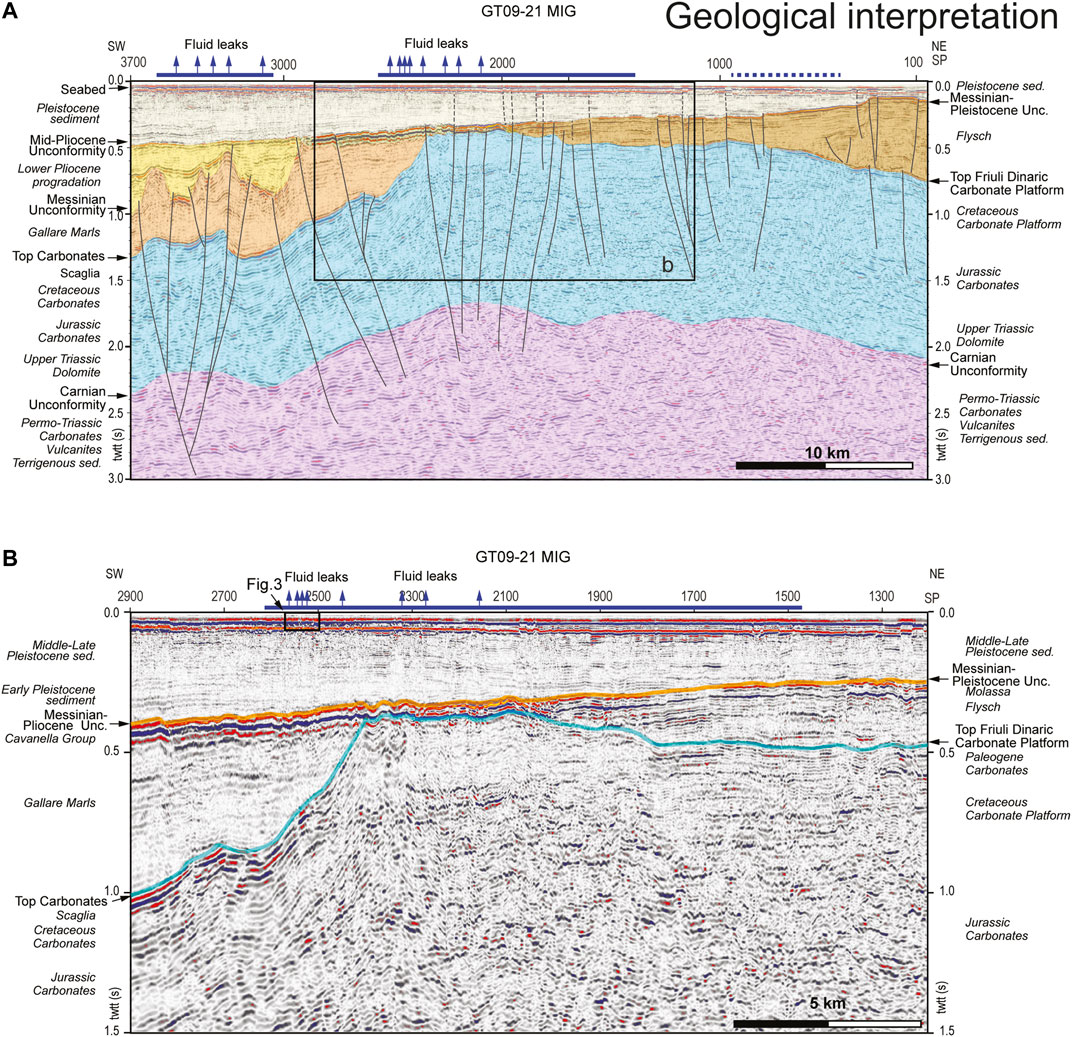
FIGURE 2. Time-migrated seismic profile GT09–21: (A) seismo-stratigraphic interpretation (see Figure 1 for location); (B) section of the seismic profile analyzed in the present work with the picked horizons. Blue lines along the profile indicate evidence of fluids within the sediment, dashed line where the fluids are less evident or discontinuous, and the blue arrows indicate the location of fluid seeps in the water column.

In subaerial conditions, the peripheral Mediterranean lands were deeply incised by canyons several km large and several hundred of meter deep (Busetti et al., 2010). In the Gulf of Trieste this event is well imaged in the seismic profiles by a high-amplitude horizon at the top the Gallare Marls, at the top of the Cavanella Group, and at the top of the turbidites of the Dinaric foredeep. The following Early Pliocene marine ingression reached only the western-most part, providing the filling of the canyons in the Gallare Marls, leaving in subaerial condition the eastern-most part. The diachronous erosional surface was progressively draped eastward by sediments during the Pleistocene (Busetti et al., 2010).

The fluids’ bearing by the rocks in the gulf have different components: brackish and fresh waters, and hydrocarbon, mainly in the gas phase (Busetti et al., 2013). The Meso-Cenozoic carbonates are characterized by permeability due to tectonic fractures and karstification that provide a confined aquifer for the geothermal reservoir. They are the reservoir of sulfurous-salty-alkaline waters at low enthalpy (about 40°C), considered to be trapped sea water of Miocene age (Petrini et al., 2013). These waters naturally spring on land in the NE coast of the gulf at the Roman Baths of Monfalcone, exploited since ancient times, and in eight submarine thermal springs in the southern offshore close to the Istria coast, with temperature from 22 to 30°C (Žumer, 2004). To exploit their geothermal potential, the Grado-1 and Grado-2 wells were drilled in 2008 and in 2015, respectively. In the Grado-1 well, water was found at 42–45°C in fractured carbonates at depths between 736 and 740 m, and from 1,040 to downhole at 1,108 m depth, while in well bottom at 1,200 m of Grado-2 well the water has 45°C with salinity more than 30‰ (Della Vedova et al., 2008; Cimolino et al., 2010; Piffer et al., 2015).

Gas seepings from the sea floor are quite common in the gulf too. Chemical analyses revealed that gas consists primarily of methane (81–84%), nitrogen (15–18%) and oxygen (0.7–1.3%). C¹⁴ datation reveals that the methane dates back to Late Pleistocene age, rising from organic rich layers, as peats (Gordini et al., 2012). Gas pockets in the shallow Late Pleistocene deposit as well as plume within the water column are well imaged by chirp data (Gordini et al., 2004; Gordini et al., 2012; Busetti et al., 2020). Fluid accumulations in the Late Pleistocene sediment are evidenced by blanking effects and high-amplitude reflectors on the top, and fluid plumes in the water column (Figure 3).

FIGURE 3

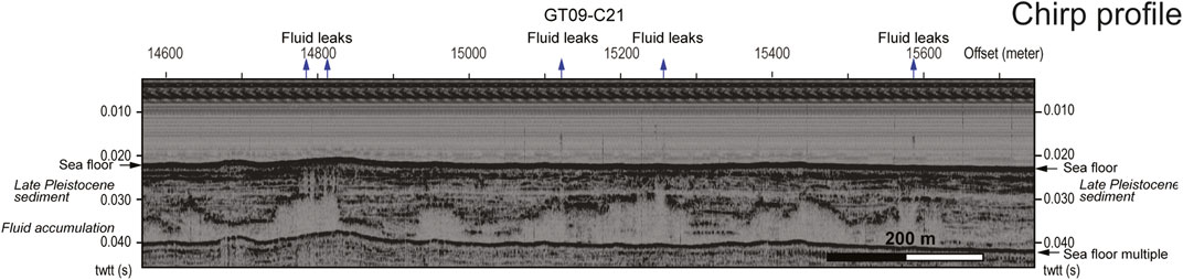
FIGURE 3. The chirp profile GT09-C21, located along the initial part of the seismic profile (see the small rectangle in Figure 2B), imaging fluid accumulation in the Late Pleistocene sediment, evidenced by the blanking effect and by the high amplitude reflectors on the top. Where the fluid migration rises very close to the sea floor, fluid plumes occur in the water column (blue arrows in the section).

Seismic Survey Parameters and Basic Processing

The data presented in this paper is part of a set of 13 multi-channel seismic profiles acquired in the Gulf of Trieste by the R/V OGS Explora in 2009, for a total length of 281 km. The seismic source is a linear array of eight sleeve guns, with a total volume of 1180 cubic inch, able to guarantee a proper penetration down to a few kilometers’ depth through the flysch and limestones hard formations, which were the original target of the survey.

The data was collected by a 96 channel, 1,200 m long digital streamer with a receiver distance of 12.5 m that, together with a shot point interval of 12.5 m, provided a nominal coverage of 48 traces per Common-Mid-Point gather. The offset between the source and the nearest channel was kept at 25 m, long enough to prevent the saturation of the recorder, but still comparable to the depth of the shallowest horizon, that is, the seafloor. Chirp profiles were collected together with the seismic data (Figure 3).

A conventional processing sequence (including deconvolution, short period seafloor multiples removal and velocity analysis) was initially adopted to produce a stack section, which was eventually migrated in depth (Figure 4). The main horizons identified in the migrated section were used as a reference to assist the picking procedure in the pre-stack domain. These horizons are indicated in the figure by arrows: the sea floor, the base of the Pleistocene sediments and the top of the carbonates.

FIGURE 4

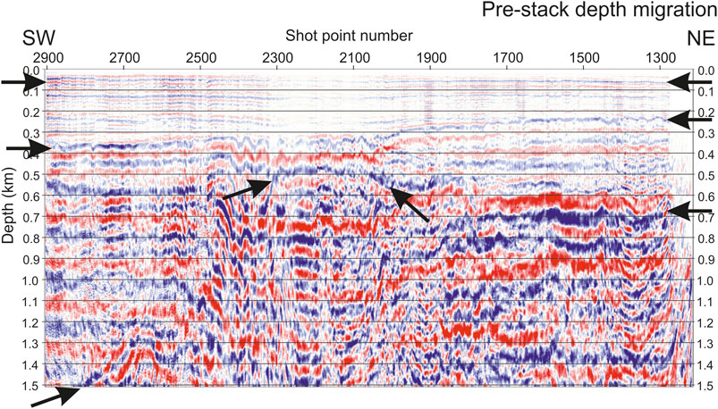
FIGURE 4. Pre-stack depth migrated section of the central part of the seismic profile GT09–21 in Figure 2.

A minimum-impact processing was applied first, consisting essentially in quality control, editing and geometry assignment. A spherical divergence compensation, based on the stacking velocities used to correct the signals in the CMP domain (Figure 5), was then applied to the pre-stack raw data, to preserve as much as possible their spectral characteristics. Indeed, the pre-processing for Q-factor imaging must not include procedures that affect heavily the signal spectrum, as bandpass filtering, Normal Move-Out (NMO) stretching, Automatic Gain Control (AGC), FX-deconvolution and even surface-consistent deconvolution. Instead, common editing (and statics, for land surveys), surface-consistent amplitude compensation or velocity-based spherical divergence recovery are fine, having a minimal impact on the frequency content. As the traveltime picking and waveform analysis are carried out in the pre-stack domain, we have not problems with the NMO stretching. After the basic processing just mentioned, the tomographic inversion of traveltimes provides a velocity model in depth. This model is used both for the pre-stack depth migration of the instantaneous frequency and for computing the Q factor from the anelastic absorption α₀ obtained by the frequency-shift tomography (Quan and Harris, 1997).

FIGURE 5

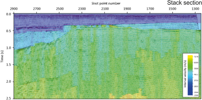
FIGURE 5. Interval velocities (colored background) derived from stacking velocities, which we used for the spherical divergence correction and the stacked time section (superimposed wiggle plot).

Complex Attributes and Anelastic Absorption

In this section, we summarize the mathematical background of broadband imaging for anelastic absorption presented by Vesnaver et al. (2016), Lin et al. (2018), to provide a critical understanding of its later application to the seismic profile.

The complex trace c(t), a function of the arrival time t, is composed of a real part r(t), which is the seismic trace recorded in the field, and of an imaginary part h(t), which is the Hilbert transform H{.} of r(t):

$c\left(t\right)=r\left(t\right)+\mathrm{i}h\left(t\right)=r\left(t\right)+\mathrm{iH}\left\{r\left(t\right)\right\}(1)$

Representing c(t) as a complex exponential, we get:

$c\left(t\right)=e\left(t\right)\exp \left[\mathrm{i}\varphi \left(t\right)\right](2)$

where:

$e\left(t\right)={\left[r{\left(t\right)}^2+h{\left(t\right)}^2\right]}^{12}=\left|c\left(t\right)\right|(3)$

$\varphi \left(t\right)=Arg\left\{c\left(t\right)\right\}(4)$

The names assigned by Taner et al. (1979) to e(t) is envelope, and to ϕ(t) is instantaneous phase. Dividing the complex trace c(t) by its envelope, which is a non-negative real function, we get the normalized complex trace n(t):

$n\left(t\right)=c\left(t\right)/e\left(t\right)=\exp \left[\mathrm{i}\varphi \left(t\right)\right],if:e\left(t\right)>0\mathrm{and}(5)$

$n\left(t\right)=0,if:e\left(t\right)=0$

Taking the time derivative of Eq. 5 and substituting (5) in the result, Poggiagliolmi and Vesnaver (2014) obtained a simple expression for the instantaneous frequency ϕ'(t), which is the time derivative of the instantaneous phase:

${\varphi }^{\prime }\left(t\right)=-\mathrm{i}n*\left(t\right)n^{\prime }\left(t\right)(6)$

where n*(t) is the complex conjugate of n(t), and n′(t) is its time derivative. According to Ackroyd (1970), Saha (1987), the value of the instantaneous frequency at the envelope extrema t_e equals the centroid of the related waveform amplitude spectrum:

${\varphi }^{\prime }\left(t_e\right)=\frac{{\displaystyle \int f A\left(f\right) df}}{{\displaystyle \int A\left(f\right) df}}(7)$

where f is the frequency and A(f) is the amplitude spectrum of the waveform surrounding the extremum point t_e.

This property may be used directly for the Q-factor tomography, as presented by Vesnaver et al. (2020), Bruno and Vesnaver (2020). In our paper, however, we exploit it to compute the high-frequency component of the anelastic absorption, to complement the low frequency part provided by reflection tomography. As the latter one is obtained in the depth domain, the next step is a depth migration of the instantaneous frequency, getting Φ(x), where x is a point in depth. The final expression for the high-frequency component of the anelastic absorption parameter A_high(x) is:

$A_{high}\left(x\right)=\frac{F}{2}\frac{\partial \mathit{\Phi }\left(\mathit{x}\right)}{\partial \mathit{z}}(8)$

where F is a real constant that depends on the seismic source spectrum. Eq. 8 defines the attribute displayed later in the example in Figure 6.

FIGURE 6

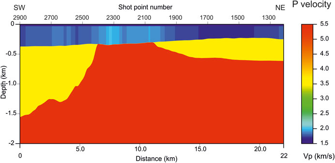
FIGURE 6. Depth migrated and derived instantaneous frequency of the line GT09–21, i.e., the high-frequency component of the anelastic absorption coefficient.

The Hilbert transform is linear, so if the substitute r(t) in (A-1) with its opposite –r(t), we get:

$-r\left(t\right)+\mathrm{i}\mathrm{H}\left\{-r\left(t\right)\right\}=-r\left(t\right)-\mathrm{i}\mathrm{H}\left\{r\left(t\right)\right\}=-\left[r\left(t\right)+\mathrm{i}\mathrm{H}\left\{r\left(t\right)\right\}\right]=-c\left(t\right)(9)$

This means that reversing the polarity of the real trace r(t), we reverse also the sign of the related complex trace. One can prove similarly that the same happens for its complex conjugate normalized trace n*(t) and the derivative n’(t) in Eq. 6. Thus, substituting r(t) with - r(t) in Eq. 6, we obtain:

$-\left[-n*\left(t\right)\right]\left[-n^{\prime }\left(t\right)\right]=-\mathrm{i}n*\left(t\right)n^{\prime }\left(t\right)={\varphi }^{\prime }\left(t\right)(10)$

i.e., the instantaneous frequency does not change when the polarity of the real trace is reversed. This is not surprising, because the same happens for the trace envelope or its amplitude spectrum. However, this invariance with respect to polarity reversals has a consequence on the anelastic absorption parameter in Eq. 8. As the derivative is linear, and the pre-stack depth migration preserves the signal polarity, this invariance applies also to the high-frequency component defined in that formula.

Tomographic Imaging

The broadband imaging we adopted is a combination of a low-resolution macro-model, including very low frequencies, and a micro-model with higher frequencies. The macro-model is obtained by reflection tomography (see, e.g., Vesnaver et al., 2000; Rossi et al., 2007, 2011) for delineating the reflecting interfaces and the P velocity. The traveltime inversion exploits a minimum-time ray tracing algorithm (Vesnaver, 1996a; Böhm et al., 1999), able to compute the ray paths of direct, reflected, refracted and diving arrivals in irregular grids.

The macro-model for anelastic absorption is estimated by the frequency-shift method by Quan and Harris (1997). The latter method is based on experimental studies of Ward and Toksöz (1971), who found that the anelastic absorption A_ray(f) along a given ray path can be expressed as a function of the frequency f as:

$A_{ray}\left(f\right)=\text{ exp}\left(-f {\displaystyle \underset{ray}{\int }{\alpha }_0 dr}\right)(11)$

where α₀ is the anelastic absorption parameter that depends on the lithology of the crossed rocks. In the most general case, absorption depends on frequency too; however, seismic surveys cover a quite limited band, as most propagating energy at significant distances ranges between 8 and 80 Hz, for standard seismic surveys. Within such a band, assuming α₀ to be frequency-independent is an acceptable approximation, used in the frequency-shift method that we adopt in this paper. Based on this assumption, we may write the following approximate equation, linking the P velocity v(x) and the anelastic absorption parameter α₀(x) to the Q factor Q(x):

$Q\left(x\right)\approx \pi /\left[v\left(x\right){\alpha }_0\left(x\right)\right](12)$

at any point x in space.

By picking reflected events (and possibly, direct and refracted arrivals too), we build a depth model for P velocity and the major layer interfaces, where the acoustic impedance contrast produces clear seismic signals. Using the waveforms surrounding the picked events, we compute the centroid of their spectrum and, comparing it with that one known of the seismic source, we can reconstruct the anelastic absorption along the ray path of picked arrivals. The obtained model is composed of a few “thick” layers only, so over-simplifying the much more complex actual layering, but getting information about the low spatial frequencies of the Earth model that otherwise is limited if using the seismic traces directly.

Figures 7, 8 show the P velocity and anelastic absorption coefficient α₀, respectively, estimated by inverting the picked traveltimes and the spectral centroids of the related waveforms. For both lithological properties, we notice some lateral variations in the uppermost sedimentary layers, just below the sea floor, i.e., in the Pleistocene sediment, while the underlying Eocene-Miocene terrigenous sediment and the Meso-Cenozoic carbonates is quite homogeneous. The lowest part presents only guessed values, as deeper reflectors could not be picked and inverted reliably. In both tomographic images, the lateral resolution is fair, i.e., about 122 m, as the final number of cells is 180, obtained by 3 staggering steps of basic grids of 60 cells. For more details about this algorithm, we send the reader to Vesnaver and Böhm (2000). Other application examples for traveltime and Q-factor tomography, using the same algorithm adopted in this paper, can be found in Vesnaver et al. (2000), Böhm et al. (2006), Rossi et al. (2007), Rossi et al. (2011), Bruno and Vesnaver (2020).

FIGURE 7

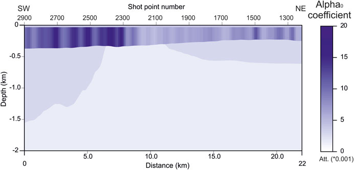
FIGURE 7. Tomographic estimation of the P velocity by the traveltime inversion of reflected arrivals from a few shallow horizons of the profile GT09–21.

FIGURE 8

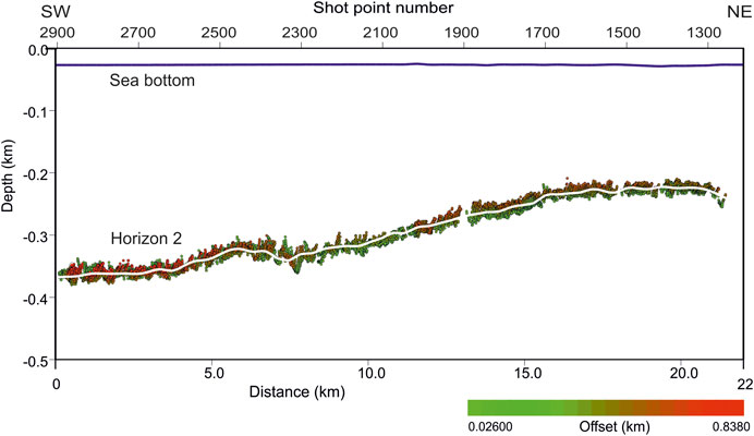
FIGURE 8. Tomographic estimation of the anelastic absorption coefficient α₀ by the local waveform analysis of reflected arrivals from a few shallow horizons of the profile GT09–21. This is the low-frequency component of the anelastic absorption.

Two picked and inverted horizons are displayed in Figures 2, 4: the sea floor and the base of Pleistocene sediment. The third one, i.e., the top of carbonates, was estimated by the pre-stack depth migration, because of the lower Signal/Noise ratio along that horizon. Due to the high fold and fair data quality, the reliability of our estimates is satisfying, and can be quantified by a few indicators. Figure 9 displays the estimated reflection points for the second horizon (the base of Pleistocene sediment). Their dispersion around the resulting interpolant line (superimposed in white) is low: the average absolute difference along the whole profile between estimated and interpolated points is about 5 m. As the average depth of that horizon is 300 m, the mismatch is lower than 2%. Another accuracy indicator is the Root Mean Square (RMS) difference between picked and modeled two-way traveltimes, which is about 1%, i.e., about 3.3 ms, close to the sampling rate. A further check is provided by the colors of the estimated reflection points: red for the far offsets, green for the near ones. When the two colors overlap, this indicates a flatness of the corresponding Common-Image gathers; when they do not do so, a residual velocity update is needed. We notice that almost everywhere along the interface this overlap is good.

FIGURE 9

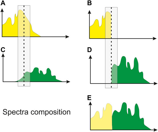
FIGURE 9. Estimated reflection points in depth for the second picked horizon, corresponding to the base of Pleistocene sediment.

Having a good fit between measured and modeled traveltimes is a necessary but not sufficient condition to get a unique, reliable solution, as many other Earth models may fit the experimental data too. This happens when a null space exists in the system of linear equations that is the core of the inversion algorithm we adopted (see, e.g., Van der Sluis and Van der Vorst, 1987). A measure for this uncertainty is the null space energy (Vesnaver, 1994; Vesnaver, 1996b), which is based on the Singular Value Decomposition (SVD) of the matrix composed of the coefficients of the linear equations. In our case, we discarded the eigen-components of the solutions’ space whose eigen-values are lower than 1% of the maximum eigen-value. The resulting local energy of the null space is mostly less than 1%: this means that 99% of the solution depends on the input data only, i.e., is only marginally affected by the initial mode choice. Such a good stability is due to the wide extension of cells (366 m) that we chose for the staggered grid inversion.

In the vertical direction, the resolution of the tomographic images in Figures 7, 8 is very limited, as the properties are constant between the reflecting interfaces, and we could pick only three major reflecting horizons. We need adding new information that could improve the vertical resolution. Picking further intermediate and deeper horizons is the ideal way, when the signal/noise ratio is good and the reflectivity continuous. This is not our case, so a different fix is required.

Broadband Imaging of Anelastic Absorption

Obtained a macro-model for P velocity and Q factor from reflection tomography, we can get the high-frequency contribution by the instantaneous frequency. This popular seismic attribute, introduced by Taner et al. (1979), can be efficiently computed without any user-defined parameter (Poggiagliolmi and Vesnaver 2014; Vesnaver 2017), i.e., by a data-driven procedure. Ackroyd (1970) proved that the instantaneous frequency is the centroid of the instantaneous spectrum of a waveform. Saha (1987) and Barnes (1991) proved that the instantaneous frequency is exactly the waveform spectral centroid at the maximum (or minimum) of its envelope. One can prove also that this is not true elsewhere (Carcione, personal communication); however, we can assume the instantaneous frequency as a reasonable proxy for the actual centroid, which is reliable only in the vicinity of the most energetic part of the seismic signal. With this caveat in mind, we will use the instantaneous frequency for complementing the low-frequency part of the anelastic absorption image obtained from seismic tomography.

The cartoon in Figure 10 explains an ideal approach for integrating macro- and micro-model. The amplitude spectra of the two components span different ranges that may partially overlap, and each of them may have a different average amplitude. We may choose part of the overlapping area where the signal energy is significant for both, and compute their average value in it. Finally, we can compensate for the amplitude value of the second spectrum by rescaling it with the inverse ratio obtained in the overlapping area, merging it with the first spectrum.

FIGURE 10

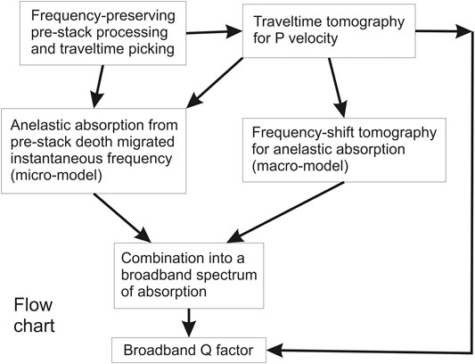
FIGURE 10. The averages of two partially overlapping spectra (A, C) are evaluated in a common window, rescaled to be similar and clipped at the window center (B, D) and merged into a single, broader spectrum.

The wider the overlapping area, the better may be relative spectra compensation, because the information from the experimental data becomes more solid from a statistical point of view. However, the overlap window should avoid the noisiest parts of the amplitude spectra, which normally are the high frequencies for the seismic signal. For the tomographic contribution, high frequencies should be avoided too, as mostly due to the Gibbs phenomenon at sharp changes of P velocity or Q factor in the blocky models we adopted. In the low frequency part, the limit is dictated mainly by the lowest values achievable by seismic sources and receivers, which are very rarely lower than a few Hz. The window choice depends so on the data quality and the parametrization of the Earth model, but also on what the interpreter assumes as signal or noise in the seismic data.

Figure 11 shows a block diagram summarizing the broadband imaging work flow. Its basic steps are:

1. Basic pre-stack processing, calculation of the instantaneous frequency and traveltime picking.

2. Traveltime inversion of direct, reflected and refracted arrivals to get a P-velocity macro-model in depth.

3. Frequency-shift tomography, using velocity and ray tracing from Step 2, getting a corresponding macro-model for the anelastic absorption parameter α₀.

4. Using the tomographic velocities from Step 2, perform a pre-stack depth migration of the instantaneous frequency from Step 1 and convert it into a micro-model for the α₀ parameter.

5. Combine micro-model from Step 4 and macro-model from Step 3 into a broadband model, carrying out a relative normalization by exploiting the possible overlapping frequency bands.

6. Convert the depth model for α₀ into a Q-factor model by using Eq. 2 and the P velocity obtained at Step 2.

FIGURE 11

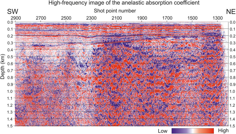
FIGURE 11. Flow chart for the broadband estimation of anelastic absorption and Q factor.

Figure 6 is the high-frequency component of the anelastic absorption, obtained as the derivative with respect to depth of the depth-migrated instantaneous frequency, defined by Eq. 8. Blue colors correspond to low absorption, while the red ones correspond to high absorption. This attribute provides only relative variations, so the scale is just qualitative without a calibration. Since the derivative is boosting the highest frequencies a lot, where the signal is much weaker than the noise, we applied a high-cut filter with a cut-off threshold of 300 Hz, as we do not expect reliable signals beyond that limit. This component highlights well two nearly flat interfaces at a depth of 120 and 190 m, which are weaker in terms of reflectivity (Figure 4), but suggest vertical discontinuities of the anelastic absorption. We note also that the horizons at 120 m depth and the sea floor are gradually dimming out when moving from left (SW) to right (NE), so detecting a lateral change of the formations’ properties.

Figure 12 shows the normalized amplitude spectra of the low-frequency component of anelastic absorption from tomography and the high-frequency component from the instantaneous frequency; both are averaged over the whole sections. We notice that the high-frequency part (blue line) approximates zero at the zero frequency and is low up to 1 Hz, where it reaches a plateau. This is due, again, to the derivative in its definition – (see Eq. 8) – as this process strongly attenuates the lowest frequencies. That part, however, is where the tomographic contribution is stronger. The area where the two components have comparable magnitude is between 4 and 16 Hz, which we selected to try a balance of the two components.

FIGURE 12

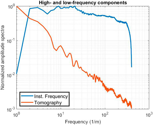
FIGURE 12. Normalized amplitude spectra of the high- and low-frequency components of the estimated anelastic absorption, in bi-logarithmic scale.

Figure 13 shows the two components and their combination in the frequency band defined by an Ormsby filter with corner frequencies 3,4,16, and 20 Hz. We notice that in the merged section (bottom), improvements are obtained in the depth range from 200 to 700 m in terms of signal continuity and sharpness. Instead, from 0 to 200 m, the part coming from tomography (top) overwhelms that one from the instantaneous frequency (center). This apparent unbalance is probably due to different noise content, which is totally absent in the tomographic component, and definitely present in the other component. Thus, the noise reduces the contribution of the signal in the high-frequency component, underweighting it if a plain energy balance is adopted to equalize the tomographic and instantaneous-frequency components. Similar effects show up when merging the full bandwidth of the two components. For this reason, we adjusted the relative weight by imposing that the highest frequency peak of the two components is nearly equal, and that there are no negative values in the resulting broadband combined absorption estimate. The result is displayed in Figure 14. The most striking difference is that there are not “negative” values any more (i.e., red colors), as the ultra-low frequencies, up to 0 Hz, are now included, provided by the tomographic contribution. When compared with the image at the bottom of Figure 13, we notice a better definition of shallow reflectors between 0 and 150 m, an improved strength and continuity of the main reflectors picked for tomography, between 200 and 600 m depth, and a decrease of the random scattering in the lowest part. The differences are visible, but not huge: probably, this is due to the extended bandwidth of the shallow signals provided by the instantaneous frequency, and the lack of usable reflectors in the deeper part. The useful signal added by the tomography is so restricted to a frequency band from 0 to 3 Hz.

FIGURE 13

FIGURE 13. Components of the estimated anelastic absorption from tomography (top) and instantaneous frequency (center) in the frequency band defined by the Ormsby filter with corner frequencies 3,4,16, and 20 Hz, and their combination (bottom), obtained by normalizing and averaging their amplitude spectra.

FIGURE 14

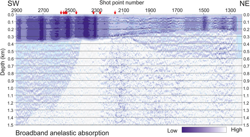
FIGURE 14. Broadband anelastic absorption, obtained combining the low-pass filtered tomographic component in Figure 8 with the high-pass filtered from the instantaneous-frequency component (Figure 6). The small red arrows on top indicate the proximity of known plume areas.

Figure 14 was obtained by choosing a real positive number for the scaling factor to balance the high- and low-frequency component. This choice is not obvious in general, as a negative factor could be chosen, in principle: the two components might be both added or subtracted. This potential ambiguity is solved by Figure 13, where we notice that, in the overlapping frequency band, the polarity of the main reflectors is the same for the two components. Thus, in this particular case, a positive sign for the scaling factor will properly sum in phase the signals from the same interface. Furthermore, comparing Figure 8 and Figure 13 (top), we understand that the blue color in Figure 13 corresponds to layers with a low absorption, as the sea water and the top of carbonates, while the red color characterizes lithologies that may be either fractured or fluid-saturated, or both, so indicating a higher absorption.

We see in Figure 14 that the shallowest 30 m, composed of sea water and unconsolidated sediments, is colored in light blue, corresponding to a low absorption. Between 40 m and over a gently dipping interface, at 350 m on the left and 210 m on the right, the absorption is higher, between the shot points 2,900 and 2,300. In the central part (shot points 2,200–1800), the absorption decreases quite sharply, while it increases again slightly in the final part, in the NE direction. Below this strong marker, up to a depth of 600 m on the right and up to the top of the carbonates on the left, we see areas of weaker and scattered signals, which have different patterns: more homogeneous on the left, where the Gallare Marls are located; characterized by patchy scatterers of increasing size in the center, where fractured and karstified carbonates are present; and a very peculiar feature on the right, where there is a slight increase in the absorption. In the central part we see that the morpho-structural high, corresponding to the paleo-shelf margin of the carbonate platform (at 350 m depth, between shot points 2,400 and 2,000) is affected by a severe blanking effect of the left flank, which is attenuated on the right side, where weak scattered, high-frequency signals show up. We interpret this difference as a major footprint of the overlying formations, which are highly absorbing on the left, and not so much on the right, or by different sedimentation environment causing progradational layers at the shelf margin, usually characterized by poorly sorted material, on the left, from the stratified inner platform carbonates on the right.

The red arrows on the top of Figure 14 indicate the locations on the known plume areas, which are located along the profile (Figure 2). Most of these plumes, located from shot points 2,600 and 2,180 correlate with the imaged anomalies. The two arrows on the left correspond to highly absorbing sedimentary units, with a lower P velocity (Figure 7). This may suggest some gas as saturating fluid. Between shot points 2,000 and 1,600, the velocity is higher and the absorption lower, which might suggest water or brine as possible saturating fluids. These hypotheses need further data collection and analysis.

Converting the anelastic absorption coefficient to the Q factor involves using Eq. 12. This is immediate when it comes to the low-frequency component provided by tomography only (Figure 15). There are lateral variations in the formations just below the sea floor, up to a depth of 300 m. Between 300 and 600 m, the variations are much lower, except for the central morpho-structural carbonate high. The deeper part is not actually inverted, as mentioned above, because of the lack to strong, continuous reflectors. As for the contributing parameters (displayed in Figures 7, 8), the vertical resolution is poor, because of the difficulty in picking additional horizons. However, a much better result is obtained when using the broadband anelastic absorption coefficient (Figure 14) instead, providing food for thought to the interpretation (Figure 16). The shallowest part (0–380 m) is almost covered by vertical gray bars on the left up to the shot point 2,200, indicating a low Q factor, while it is populated by a few reflectors in the remaining part. The interfaces between the interpreted horizons are a bit sharper. Remarkable is the signal continuity at 300 m depth, which is strong from the central horst-like structure to the left, while it is fainter toward the right side. The difference between these two parts suggests different petrophysical properties for the underlying lithologies. This clue is strengthened by the different seismic stratigraphy of the two lithologies: on the left, composed of scattered signals with medium frequencies; on the right, characterized by a few low-frequency reflectors. Below the picked horizons, the signal is discontinuous and randomly scattered, in a different way in the three parts (left, center, right) of the carbonates. As mentioned above, these differences may be a footprint of the overlying different formations.

FIGURE 15

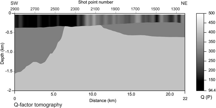
FIGURE 15. Q factor estimation obtained by P velocity in Figure 7 and the anelastic absorption coefficient in Figure 8. This result is the low-frequency component, based on tomography only.

FIGURE 16

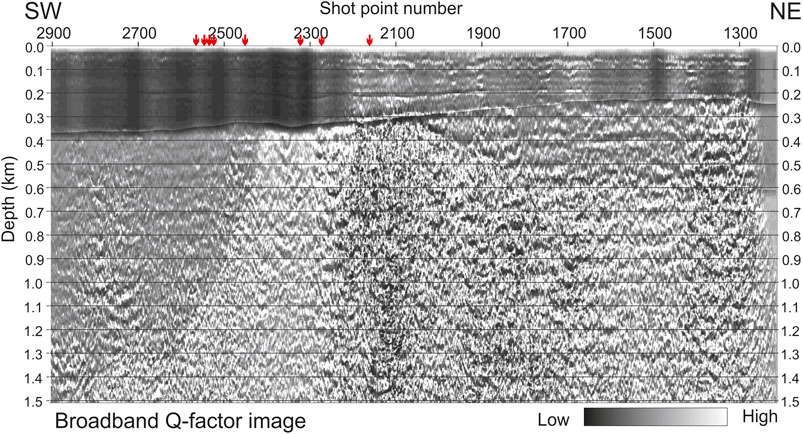
FIGURE 16. Q factor estimation obtained by P velocity in Figure 7 and the broadband anelastic absorption coefficient in Figure 6. The small red arrows on top indicate the proximity of known plume areas.

As for Figure 13 and other similar ones, the color scale is qualitative only, because without a well calibration, the high-frequency component and its percentage contribution to the final broadband estimate (Figure 16) depend on acquisition and user-defined processing parameters. Although the latter ones are bounded by physical constraints and geological knowledge about rock properties, at this stage our estimation is only semi-quantitative.

Geological Remarks

The most evident result of the absorption model within the Pleistocene sediment, with high absorption in the western part, low in the central part, and medium in the eastern part (Figure 14), could reflect the occurring of the different phases and components of the fluids present in the study area.

Seismic facies of the Late Pleistocene sediment in the seismic profiles and in the high-resolution chirp data (Figure 2) show the occurrence of fluids and fluid seepages at the sea floor, that sample analysis revealed to be mainly methane of biogenic origin (Busetti et al., 2020; Gordini et al., 2004; Gordini et al., 2012). From the correlation between seismic and Chirp data, the main area with gas bearing sediments results in the western part of the analyzed profiles. The western Gulf of Trieste is rich of sites related to gas seepages (Gordini et al., 2003) and some of them are quite close the analyzed profiles. Chirp data permits identifying some plume sites (Figure 2), but gas seepages nearby could be significantly more than those ones recognized. These evidences suggest that the high absorption within the Pleistocene sediment in the western part of the profile (Figure 14) could reflect the occurrence of gas.

The carbonate units are the confined reservoir of trapped Miocene sea water (Petrini et al., 2013). The sonic log acquired in the Grado-2 well indicates that the Paleogene carbonates, located in the eastern upper few hundred-meter part of the carbonate platform, are characterized by more fractures and stratification than the Cretaceous limestone, being potentially a more efficient reservoir (Piffer et al., 2015). The carbonate reservoir is sealed on the east by the turbiditic units of the Eocene flysch and by the terrigenous Miocene Molasse, while in correspondence of the morpho-structural high, the carbonates are draped by about 100 m of the Miocene Cavanella Group composed of sand, sandstones and marls (Nicolich et al., 2004). The Cavanella Group, occurring in the Friulian Plain, thins southward pinching out in the Gulf of Trieste. Hence, thinning southward, the Cavanella Group loose progressively the capacity to be an efficient seal, and the salty waters may migrate upward, in the Pleistocene sediment. This hypothesis could explain the low absorption zone in correspondence of the Pleistocene sediment lying above the eastern part of the morpho-structural carbonate high. The medium absorption in the eastern part could be related to less evident gas occurrence within the sediment.

Discussion

The broadband imaging method presented in this paper is a heuristic approach, based on a few major approximations. Thus, we should regard it as a semi-quantitative tool, able to highlight local lithology variations, but not providing a precise measurement to be used for direct engineering applications. Within these premises, however, it is a clear advance with respect to current technologies in terms of spatial resolution for detecting saturated formations and fluid pathways. Using synthetic seismograms (and thus known models), Vesnaver and Lin (2019) showed that this method works nicely also when the acoustic impedance contrast is modest in a hydrocarbon reservoir, so that the oil/water contact cannot be detected by a standard approach. However, if a production technique as fracking is applied, the rock matrix is affected and the Q factor decreases: then, it becomes a good parameter to delineate fracked regions and optimize the production of hydrocarbons or geothermal energy.

Some heuristic methods have been used effectively. A similar approach to our one was introduced for a broadband estimation of the acoustic impedance by Lindseth (1976), Lavergne and Willm (1977) and Becquey et al. (1979), getting successful applications for decades in oil and gas exploration. Other comparable hybrid methods were presented by Mora (1989) for seismic reflectivity and by Tura et al. (1998) for the depth conversion of attributes derived by Amplitude vs. Offset analysis.

We remark that the absorption images highlight the relative contrast of this property among different formations illuminated by the seismic waves, and not absolute values. This applies to both low- and high-frequency components. For the tomographic contribution, the adopted method of Quan and Harris (1997) assumes a few hypotheses, as a white spectrum for the Earth reflectivity, which can be violated in real experiments. Vesnaver et al. (2020) showed that a calibration by well logs can fix such a drawback, but when such information is missing (as in our test case), we must be aware that our results might need to be adjusted by a scaling factor. Another scaling factor is needed to calibrate the high-frequency component, as it is dependent on the frequency band spanned by the seismic source. Thus, the relative weight of high- and low-frequency component may be just guessed, within physical constraints, unless a well calibration is available to consolidate both items.

The improvement in the broadband Q-factor estimation vs. the purely tomographic one is dramatic, but suffers a weakness: the tomographic velocity field is available only at a low-resolution. Ideally, the high-resolution version should be provided a full-waveform inversion, may be even just with an acoustic implementation. We expect significant improvements in this case, which is left to further studies.

The frequency band of seismic signals is limited: in the chase history presented here, it ranges from a few Hz to over 200 Hz (Figure 12). The lowest missing frequencies (from 0 to a few Hz) correspond to the averages of velocity and absorption, which are the zero frequency, and to the linear trend of their values. The traveltime inversion estimates the absolute values of P velocities: it is very amenable for injecting “a priori” information in the inversion process, as physical limits for acceptable velocities and a certain smoothness level for their later variations. Furthermore, an increasing trend is expected for both P velocity and Q factor in most cases, due to the increasing lithostatic load as a function of depth. This additional information is a key contribution for filling the low-frequency gap for P velocities and the main interfaces’ structure. When it comes to anelastic absorption (or Q factor), this gap is filled properly only if a calibration by well logs is available (see Vesnaver et al., 2020). If this data is missing, as in our case study, we may use only more general constraints: for example, high Q values in the sea water and much lower ones in unconsolidated sea floor sediments. In the latter case, however, the result is semi-quantitative only: as just the relative contrasts are data driven, the absolute values may be biased by the chosen constraints.

Conclusion

The broadband estimation of anelastic absorption is an effective tool for characterizing fractures or fluid-saturated formations, or both. We tested this recent method on a marine survey acquired in the Gulf of Trieste (Italy) to validate a few geological hypotheses about fluid occurrence within the sediment and emissions at the sea floor. We hypothesize that the high absorption of the Pleistocene sediment is related to biogenic gas occurrence, while the low absorption zones are reasonably correlated to possible migration of salty water from deep carbonate reservoir to the Miocene-Pleistocene sediment.

Data Availability Statement

The raw data supporting the conclusions of this article will be made available by the authors, without undue reservation.

Author Contributions

AV prepared the basic manuscript and developed the algorithm for the broadband imaging. GB carried out the tomographic inversion of P velocity and Q factor, and the related pre-stack depth migration. MDC and MB cared the geological setting and interpreted the seismic data. MB managed the project for the data acquisition and interpretation. FZ acquired the seismic data and completed its basic processing. All authors contributed to the final discussion and the manuscript editing and revision.

Funding

Our work was supported by the National Institute of Oceanography and Applied Geophysics – OGS, in the framework of the projects “Geological and tectonic evolution of the Gulf of Trieste (N-Adriatic)”, supported by OGS.

Conflict of Interest

The authors declare that the research was conducted in the absence of any commercial or financial relationships that could be construed as a potential conflict of interest.

Acknowledgments

We acknowledge our colleagues that contributed to the seismic data acquisition by the vessel OGS-Explora. We acknowledge IHS Markit® and Schlumberger® that provided to OGS the academic Kingdom® and Vista® software licenses.

References

Ackroyd, M. H. (1970). Instantaneous spectra and instantaneous frequency. Proc. IEEE 58, 141. doi:10.1109/proc.1970.7552

CrossRef Full Text | Google Scholar

Agudo, Ò. C., da Silva, N. V., Warner, M., Morgan, J., and Morgan, J. (2018). Acoustic full-waveform inversion in an elastic world. Geophysics 83, R257–R271. doi:10.1190/geo2017-0063.1

CrossRef Full Text | Google Scholar

Arso (2017). Ministry of the environment and spatial planning, Slovenian environment agency. Available at: https://gis.arso.gov.si (Accessed April 5, 2017).

Google Scholar

Ba, J., Carcione, J. M., and Sun, W. (2015). Seismic attenuation due to heterogeneities of rock fabric and fluid distribution. Geophys. J. Int. 202, 1843–1847. doi:10.1093/gji/ggv255

CrossRef Full Text | Google Scholar

Bai, T., Tsvankin, I., and Wu, X. (2017). Waveform inversion for attenuation estimation in anisotropic media. Geophysics 82, WA83–WA93. doi:10.1190/geo2016-0596.1

CrossRef Full Text | Google Scholar

Barnes, A. E. (1991). Instantaneous frequency and amplitude at the envelope peak of a constant‐phase wavelet. Geophysics 56, 1058–1060. doi:10.1190/1.1443115

CrossRef Full Text | Google Scholar

Becquey, M., Lavergne, M., and Willm, C. (1979). Acoustic impedance logs computed from seismic traces. Geophysics 44, 1485–1501. doi:10.1190/1.1441020

CrossRef Full Text | Google Scholar

Best, A. I., McCann, C., and Sothcott, J. (1994). The relationships between the velocities, attenuations and petrophysical properties of reservoir sedimentary rocks1. Geophys. Prospect. 42, 151–178. doi:10.1111/j.1365-2478.1994.tb00204.x

CrossRef Full Text | Google Scholar

Böhm, G., Rossi, G., and Vesnaver, A. (1999). Minimum time ray tracing for 3D irregular grids. J. Seism. Explor. 8, 117–131.

Google Scholar

Böhm, G., Accaino, F., Rossi, G., and Tinivella, U. (2006). Tomographic joint inversion of first arrivals in a real case from Saudi Arabia. Geophys. Prospect. 54, 721–730. doi:10.1111/j.1365-2478.2006.00563.x

CrossRef Full Text | Google Scholar

Bruno, P. P., and Vesnaver, A. (2020). Groundwater characterization in arid regions using seismic and gravity attributes: Al Jaww Plain, UAE. Front. Earth Sci. 8, 575019. doi:10.3389/feart.2020.575019

CrossRef Full Text | Google Scholar

Busetti, M., Babich, A., and Del Ben, A. (2020). Geophysical evidence of fluids emission in the gulf of Trieste (North Adriatic Sea). Mem. Descr. Carta Geol. d’Italia 105, 11–16.

Google Scholar

Busetti, M., Volpi, V., Nicolich, R., Barison, E., Romeo, R., Baradello, L., et al. (2010). Dinaric tectonic features in the gulf of Trieste (Northern Adriatic). Boll. Geof. Teor. Appl. 51 (2–3), 117–128.

Google Scholar

Busetti, M., Zgur, F., Vrabec, M., Facchin, L., Pelos, C., Romeo, R., et al. (2013). “Neotectonic reactivation of Meso-Cenozoic structures in the Gulf of Trieste and its relationship with fluid seepings,” in Proceedings of the 32nd gruppo nazionale di geofisica della terra solida (GNGTS) congress, Rome, Italy, November 19–21, 2013 (Trieste, Italy: GNGTS), 29–34.

Google Scholar

Carcione, J. M. (2014). Wave Fields in Real Media. Theory and numerical simulation of wave propagation in anisotropic, anelastic, porous and electromagnetic media. 3rd Edn. Amsterdam, Netherlands: Elsevier, 690.

Casero, P. (2004). Structural setting of petroleum exploration plays in Italy. Geology of Italy: special volume of the Italian geological society for the international geological congress 32, Florence, Italy, August 20–28, 2004 (Florence, Italy: International Geological Congress), 189–199.

Google Scholar

Cheng, P., and Margrave, G. F. (2012). “Q estimation by a match-filter method,” in Expanded Abstracts, SEG Annual Meeting, Las Vegas, Nevada, November 4–9, 2012 (Las Vegas, Nevada: SEG), 1–5.

Google Scholar

Cimolino, A., Della Vedova, B., Nicolich, R., Barison, E., and Brancatelli, G. (2010). New Evidence of the outer Dinaric deformation front in the Grado area (NE-Italy). Rend. Fis. Acc. Lincei 21 (Suppl. 1), 167–179. doi:10.1007/s12210-010-0096-y

CrossRef Full Text | Google Scholar

Conti, A., Stefanon, A., and Zuppi, G. M. (2002). Gas seeps and rock formation in the northern Adriatic Sea. Cont. Shelf Res. 22, 2333–2344. doi:10.1016/s0278-4343(02)00059-6

CrossRef Full Text | Google Scholar

Cucchi, F., Piano, C., Fanucci, C. F., Pugliese, N., Tunis, G., et al. (2013). Brevi Note Illustrative della Carta Geologica del Carso Classico Italiano. Friuli Venezia Giulia: Progetto GEO-CGT, 43. Available at: http://www.regione.fvg.it/rafvg/cms/RAFVG/ambiente-territorio/tutela-ambiente-gestione-risorse-naturali/ (Accessed April 2016).

Della Vedova, B., Castelli, E., Cimolino, A., Vecellio, C., Nicolich, R., and Barison, E. (2008). La valutazione e lo sfruttamento delle acque geotermiche per il riscaldamento degli edifici pubblici. Rassegna Tecnica Del. Friuli Venezia Giulia 6, 16–19.

Google Scholar

Donda, F., Tinivella, U., Gordini, E., Panieri, G., Volpi, V., and Civile, D. (2019). The origin of gas seeps in the Northern Adriatic Sea. Italian J. Geosci. 138 (2), 171.183. doi:10.3301/IJG.2018.34

Google Scholar

EMODnet Digital Bathymetry (2018). EMODnet bathymetry consortium. Available at: https://www.emodnet.eu (Accessed September 14, 2018).

Google Scholar

EU-DEM (2017). Copernicus land monitoring service. Available at: https://www.eea.europa.eu/data-and-maps/data/copernicus-land-monitoring-service-eu-dem (Accessed December 7, 2017).

Google Scholar

Geletti, R., Del Ben, A., Busetti, M., Ramella, R., and Volpi, V. (2008). Gas seeps linked to salt structures in the Central Adriatic Sea. Basin Res. 20, 473–487. doi:10.1111/j.1365-2117.2008.00373.x

CrossRef Full Text | Google Scholar

Gordini, E., Caressa, S., and Marocco, R. (2003). New morpho-sedimentological map of the Trieste Gulf (from punta tagliamento to isonzo mouth). Atti Del. Museo Friulano di Storia Nat. 35, 5–29. doi:10.1016/j.quaint.2007.08.044

CrossRef Full Text | Google Scholar

Gordini, E., Marocco, R., Tunis, G., and Ramella, R. (2004). I depositi cementati del Golfo di Trieste (Adriatico Settentrionale): distribuzione areale, caratteri geomorfologici e indagini acustiche ad alta risoluzione. Il Quaternario 17 (2/2), 555–563.

Google Scholar

Gordini, E., Falace, A., Kaleb, S., Donda, F., Marocco, R., and Tunis, G. (2012). “Methane-related carbonate cementation of marine sediments and related macroalgal coralligenous assemblages in the northern Adriatic Sea,” in Seafloor geomorphology as benthic habitats. Editors P. T. Harris, and E. K. Baker (Amsterdam, Netherlands: Elsevier), 183–198.

Google Scholar

Hackert, C. L., and Parra, J. O. (2003). Estimating scattering attenuation from vugs or karsts. Geophysics 68, 1182–1188. doi:10.1190/1.1598111

CrossRef Full Text | Google Scholar

Helle, H. B., Pham, N. H., and Carcione, J. M. (2003). Velocity and attenuation in partially saturated rocks: poroelastic numerical experiments. Geophys. Prospect. 51, 551–566. doi:10.1046/j.1365-2478.2003.00393.x

CrossRef Full Text | Google Scholar

Hovland, M., and Curzi, P. V. (1989). Gas seepage and assumed mud diapirism in the Italian central Adriatic Sea. Mar. Pet. Geol. 6, 161–169. doi:10.1016/0264-8172(89)90019-6

CrossRef Full Text | Google Scholar

IRDAT-FVG (2017). Infrastruttura Regionale di Dati Ambientali e Territoriali per il Friuli Venezia Giulia. Available at: https://irdat.regione.fvg.it/WebGIS/ (Accessed September 8, 2012).

Google Scholar

Jannsen, D., Voss, J., and Theilen, F. (1985). Comparison of methods to determine Q in shallow marine sediments from vertical reflection seismograms*. Geophys. Prospect. 33, 479–497. doi:10.1111/j.1365-2478.1985.tb00762.x

CrossRef Full Text | Google Scholar

Jurkovšek, B., Biolchi, S., Furlani, S., Kolar-Jurkovšek, T., Zini, L., Jež, J., et al. (2016). Geology of the classical Karst region (SW Slovenia–NE Italy). J. Maps 12, 352–362. doi:10.1080/17445647.2016.1215941

CrossRef Full Text | Google Scholar

Lavergne, M., and Willm, C. (1977). Inversion of seismograms and pseudo-velocity logs. Geophys. Prospect. 25, 232–250. doi:10.1111/j.1365-2478.1977.tb01165.x

CrossRef Full Text | Google Scholar

Lin, R., Vesnaver, A., Böhm, G., and Carcione, J. M. (2018). Broad-band viscoacoustic Q-factor imaging by seismic tomography and instantaneous frequency. Geophys. J. Int. 214, 672–686. doi:10.1093/gji/ggy168

CrossRef Full Text | Google Scholar

Lindseth, R. O. (1976). Seislog process uses seismic reflection traces. Oil Gas J. 38, 481–488.

Google Scholar

Mora, P. (1989). Inversion = migration + tomography. Geophysics 54, 1575–1586. doi:10.1190/1.1442625

CrossRef Full Text | Google Scholar

Mulder, W. A., and Hak, B. (2009). An ambiguity in attenuation scattering imaging. Geophys. J. Int. 178, 1614–1624. doi:10.1111/j.1365-246x.2009.04253.x

CrossRef Full Text | Google Scholar

Nicolich, R., Della Vedova, B., Giustiniani, M., and Fantoni, R. (2004). Carta del sottosuolo della Pianura Friulana (Map of subsurface of the Friuli Plain). LAC-Firenze, Italy. RAFVG–UNITS-DIC, 32.

Petrini, R., Italiano, F., Ponton, M., Slejko, F. F., Aviani, U., and Zini, L. (2013). Geochemistry and isotope geochemistry of the Monfalcone thermal waters (Northern Italy): inference on the deep geothermal reservoir. Hydrogeol. J. 21, 1275–1287. doi:10.1007/s10040-013-1007-y

CrossRef Full Text | Google Scholar

Picotti, S., and Carcione, J. M. (2006). Estimating seismic attenuation (Q) in the presence of random noise. J. Seism. Explor. 15, 165–181.

Google Scholar

Piffer, G., Rinaldi, M., and Della Vedova, B. (2015). “Well logging for the geothermal reservoir characterization: the Grado geothermal project (Gorizia, Italy)–Part 2,” in Proceedings of the geo alp kongress–geologie und hydrogeologie der alpen–geologia e idrogeologia della alpi, Gorizia, Italy, November 5–7, 2015 (Fortezza, Italy: Ordine dei Geologi Regione del Veneto), 2. Available at: http://www.waterstones-srl.it/wp-content/uploads/2015/11/100x80-A-B.pdf.

Google Scholar

Placer, L., Vrabec, M., and Celarc, B. (2010). The bases for understanding of the NW Dinarides and Istria Peninsula tectonics. Geologija 53, 55–86. doi:10.5474/geologija.2010.005

CrossRef Full Text | Google Scholar

Poggiagliolmi, E., and Vesnaver, A. (2014). Instantaneous phase and frequency derived without user-defined parameters. Geophys. J. Int. 199, 1544–1553. doi:10.1093/gji/ggu352

CrossRef Full Text | Google Scholar

Quan, Y., and Harris, J. M. (1997). Seismic attenuation tomography using the frequency shift method. Geophysics 62, 895–905. doi:10.1190/1.1444197

CrossRef Full Text | Google Scholar

Rossi, G., Gei, D., Böhm, G., Madrussani, G., and Carcione, J. M. (2007). Attenuation tomography: an application to gas-hydrate and free-gas detection. Geophys. Prospect. 55, 655–669. doi:10.1111/j.1365-2478.2007.00646.x

CrossRef Full Text | Google Scholar

Rossi, G., Chadwick, R. A., and Williams, G. A. (2011). “Traveltime and attenuation tomography of CO₂ plume at Sleipner,” in Expanded abstracts, EAGE annual meeting, Vienna, Austria, May 23–26 2011 (EAGE), A039.

Google Scholar

Saha, J. G. (1987). “Relationship between Fourier and instantaneous frequency,” in Expanded abstracts, SEG annual meeting, (SEG), 591–594.

Google Scholar

Shapiro, S., and Hubral, P. (1999). Elastic waves in random media. Berlin, Germany: Springer, 191.

Song, Y., Hu, H., and Han, B. (2020a). Seismic attenuation and dispersion in a cracked porous medium: an effective medium model based on poroelastic linear slip conditions. Mech. Mater. 140, 103229. doi:10.1016/j.mechmat.2019.103229

CrossRef Full Text | Google Scholar

Song, Y., Rudnicki, J. W., Hu, H., and Han, B. (2020b). Dynamics anisotropy in a porous solid with aligned slit fractures. J. Mech. Phys. Solids 137, 103865. doi:10.1016/j.jmps.2020.103865

CrossRef Full Text | Google Scholar

Taner, M. T., Koehler, F., and Sheriff, R. E. (1979). Complex seismic trace analysis. Geophysics 44, 1041–1063. doi:10.1190/1.1440994

CrossRef Full Text | Google Scholar

Tonn, R. (1991). The determination of the seismic quality factor Q from vsp data: a comparison of different computational Methods1. Geophys. Prospect. 39, 1–27. doi:10.1111/j.1365-2478.1991.tb00298.x

CrossRef Full Text | Google Scholar

Trobec, A., Busetti, M., Zgur, F., Baradello, L., Babich, A., Cova, A., et al. (2018). Thickness of marine holocene sediment in the Gulf of Trieste (Northern Adriatic Sea). Earth Syst. Sci. Data 10, 1077–1092. doi:10.5194/essd-10-1077-2018

CrossRef Full Text | Google Scholar

Tura, A., Hanitzsch, C., and Calandra, H. (1998). 3-D AVO migration/inversion of field data. Lead. Edge 17, 1578. doi:10.1190/1.1437898

CrossRef Full Text | Google Scholar

Van der Sluis, A., and Van der Vorst, H. A. (1987). “Numerical solution of large, sparse linear algebraic systems arising from tomographic problems,” in Seismic tomography with applications in global seismology and exploration geophysics. Editor G. Nolet (Dordrecht: Reidel), 49–83.

CrossRef Full Text | Google Scholar

Vesnaver, A. (1994). Towards the uniqueness of tomographic inversion solutions. J. Seism. Explor. 3, 323–334.

Google Scholar

Vesnaver, A. (2017). Instantaneous frequency and phase without unwrapping. Geophysics 82, F1–F7. doi:10.1190/geo2016-0185.1

CrossRef Full Text | Google Scholar

Vesnaver, A. (1996a). The contribution of reflected, refracted and transmitted waves to seismic tomography: a tutorial. First Break 14, 159–168. doi:10.3997/1365-2397.1996010

CrossRef Full Text | Google Scholar

Vesnaver, A. L. (1996b). Ray tracing based on Fermat's principle in irregular grids1. Geophys. Prospect. 44, 741–760. doi:10.1111/j.1365-2478.1996.tb00172.x

CrossRef Full Text | Google Scholar

Vesnaver, A., and Böhm, G. (2000). Staggered or adapted grids for seismic tomography?. Lead. Edge 19, 944–950. doi:10.1190/1.1438762

CrossRef Full Text | Google Scholar

Vesnaver, A., Böhm, G., Madrussani, G., Rossi, G., and Granser, H. (2000). Depth imaging and velocity calibration by 3D adaptive tomography*. First Break 18, 303–312. doi:10.1046/j.1365-2397.2000.00093.x

CrossRef Full Text | Google Scholar

Vesnaver, A., Lin, R., and Böhm, G. (2016). Merging macro- and micro-models for a broadband estimation of the Q factor. Soc. Explor. Geophys., 3613–3617. doi:10.1190/segam2016-13859201.1

CrossRef Full Text | Google Scholar

Vesnaver, A., Böhm, G., Cance, P., Dal Cin, M., and Gei, D. (2020). Windowless Q‐factor tomography by the instantaneous frequency. Geophys. Prospect. 68, 2611–2636. doi:10.1111/1365-2478.13020

CrossRef Full Text | Google Scholar

Vesnaver, A., and Lin, R. (2019). Broadband Q-factor tomography for reservoir monitoring. J. Appl. Geophys. 165, 1–15. doi:10.1016/j.jappgeo.2019.04.004

CrossRef Full Text | Google Scholar

Ward, R. W., and Toksöz, M. N. (1971). Causes of regional variation of magnitude. Bull. Seismol. Soc. Am. 61, 649–670.

Google Scholar

Wu, R.-S. (1985). Multiple scattering and energy transfer of seismic waves–separation of scattering effect from intrinsic attenuation–I. Theoretical modelling. Geophys. J. Int. 82, 57–80. doi:10.1111/j.1365-246x.1985.tb05128.x

CrossRef Full Text | Google Scholar

Zampa, L. S. (2020). Technical Report 05/2020OGS. New bathymetric maps of the north east Adriatic Sea. Available at: https://www2.eecs.berkeley.edu/Pubs/TechRpts/ (Accessed October 5, 2020).

Google Scholar

Žumer, J. (2004). Odkritje podmorskih termalnih izvirov. Geografski Obzornik 51, 11–17.

Google Scholar