 Amir Sadeghi-Bagherabadi1,2*
 Alessandro Vuan1
 Abdelkrim Aoudia2
 Stefano Parolai1The AlpArray and AlpArray-Swath-D Working Group
- 1National Institute of Oceanography and Applied Geophysics–OGS, Trieste, Italy
- 2Earth System Physics Section, Abdus Salam International Centre for Theoretical Physics–ICTP, Trieste, Italy
We compiled a dataset of continuous recordings from the temporary and permanent seismic networks to compute the high-resolution 3D S-wave velocity model of the Southeastern Alps, the western part of the external Dinarides, and the Friuli and Venetian plains through ambient noise tomography. Part of the dataset is recorded by the SWATH-D temporary network and permanent networks in Italy, Austria, Slovenia and Croatia between October 2017 and July 2018. We computed 4050 vertical component cross-correlations to obtain the empirical Rayleigh wave Green’s functions. The dataset is complemented by adopting 1804 high-quality correlograms from other studies. The fast-marching method for 2D surface wave tomography is applied to the phase velocity dispersion curves in the 2–30 s period band. The resulting local dispersion curves are inverted for 1D S-wave velocity profiles using the non-perturbational and perturbational inversion methods. We assembled the 1D S-wave velocity profiles into a pseudo-3D S-wave velocity model from the surface down to 60 km depth. A range of iso-velocities, representing the crystalline basement depth and the crustal thickness, are determined. We found the average depth over the 2.8–3.0 and 4.1–4.3 km/s iso-velocity ranges to be reasonable representations of the crystalline basement and Moho depths, respectively. The basement depth map shows that the shallower crystalline basement beneath the Schio-Vicenza fault highlights the boundary between the deeper Venetian and Friuli plains to the east and the Po-plain to the west. The estimated Moho depth map displays a thickened crust along the boundary between the Friuli plain and the external Dinarides. It also reveals a N-S narrow corridor of crustal thinning to the east of the junction of Giudicarie and Periadriatic lines, which was not reported by other seismic imaging studies. This corridor of shallower Moho is located beneath the surface outcrop of the Permian magmatic rocks and seems to be connected to the continuation of the Permian magmatism to the deep-seated crust. We compared the shallow crustal velocities and the hypocentral location of the earthquakes in the Southern foothills of the Alps. It revealed that the seismicity mainly occurs in the S-wave velocity range between ∼3.1 and ∼3.6 km/s.
Introduction
The Eastern Alps and external Dinarides across North-Eastern Italy, Austria and Western Slovenia are the result of the collision between the European plate with the Adriatic microplate (e.g., Dewey et al., 1989). Their evolution since Late Cretaceous is mainly controlled by the protrusion of the Adriatic lower crust (e.g., Handy et al., 2010), a relatively rigid and less deformed continental crustal block pushed into weaker parts of the orogen. The Adria microplate, squeezed between the African and European plates, is rotating counterclockwise relatively to Eurasia (e.g., Serpelloni et al., 2005; Le Breton et al., 2017) and its indentation is accommodated by NNW-SSE shortening in the Eastern and Southern Alps. The Eastern Alps and the Southeastern Alps show a complex structure reflecting the interplay between orogen-normal shortening and orogen-parallel motion (e.g., Handy et al., 2015).
The seismicity is mainly located in the upper-middle crust and along the Southeastern Alps foothills (Viganò et al., 2015; Bressan et al., 2016). Fault mechanisms show a compression from NW-SE to N-S, and NNE-SSW, consistent with the geodynamic setting, and seismicity patterns seem to be controlled by the crustal heterogeneities and the different degree of interseismic coupling along the main thrust front.
Seismic experiments carried out during the last two decades, TRANSALP (TRANSALP Working Group, 2002), ALP 2002 (Brückl et al., 2007; Grad et al., 2009; Šumanovac et al., 2009), and CROP (Finetti, 2005) suggested the subduction of Eurasia below the Adria microplate to the west of the Southeastern Alps below the Tauern Window. From the Tauern window to the east, a sudden change in the subduction direction is inferred from teleseismic tomography studies (e.g., Kissling et al., 2006; Handy et al., 2015), and the interaction of the Adriatic microplate and Eurasia is made more complex by its underthrusting below the Dinarides and the Pannonian fragment (Brückl et al., 2010; Šumanovac et al., 2016). The Eastern Alps structural complexity and the existing different tectonic models triggered in the last decade a number of studies on crustal and upper mantle structure, also made possible by the development of more dense seismological networks in the area (AlpArray Seismic Network, 2015; Istituto Nazionale Di Oceanografia E Di Geofisica Sperimentale, 2016; Hetényi et al., 2018a).
By using permanent and temporary stations, seismic tomography studies were carried out at continental and regional scales (e.g., Molinari et al., 2015; Behm et al., 2016; Guidarelli et al., 2017; Tondi et al., 2019). A recent joint inversion of surface wave phase velocities from ambient noise and earthquakes confirmed the heterogeneity of the crustal structure between the Central and Eastern Alps (Kästle et al., 2018). New crustal models from ambient noise tomography have also been recently proposed by Lu et al. (2020), Molinari et al. (2020), Qorbani et al. (2020) improving the resolution of the existing reference models like EPcrust (Molinari and Morelli, 2011).
Receiver function data and the global-phase seismic interferometry, provided by the AlpArray complementary experiment EASI (Hetényi et al., 2018b; Kvapil et al., 2020), with focus on the Eastern Alps, highlighted a complex crustal structure and suggested a possible Adria subduction below Eurasia (Hetényi et al., 2018b; Bianchi et al., 2020). However, the interpretation of the receiver function data is still ambiguous due to the possible presence of slices of lower crust imbricated at the contact between Eurasia and Adria, and therefore not a single interface at depth with an overall acoustic impedance (Bianchi and Bokelmann, 2014; Bianchi et al., 2015).
For mapping in greater detail the Moho discontinuity, investigating its possible fragmentation, and improving the knowledge about the dynamic processes that originated crustal growth, accretion, delamination, and underplating, an array of 154 broadband seismic stations (Figure 1, AlpArray-SWATH-D project) in the Eastern Alpine region was completed at the end of 2017 and operated for 2 years (Heit et al., 2017). SWATH-D focuses on a key area of the Alps where the hypothesized flip in the subduction polarity is suggested to occur and where the TRANSALP experiment has imaged a jump in the Moho geometry (TRANSALP Working Group, 2002). The temporary network complemented the larger-scale AlpArray network and existing permanent stations of the Alps-Adria region (Heit et al., 2017). The spatial density of the integrated seismic networks provides the opportunity to improve the lateral resolution for ambient noise and receiver function studies, including greater detail in the crustal and uppermost mantle models.
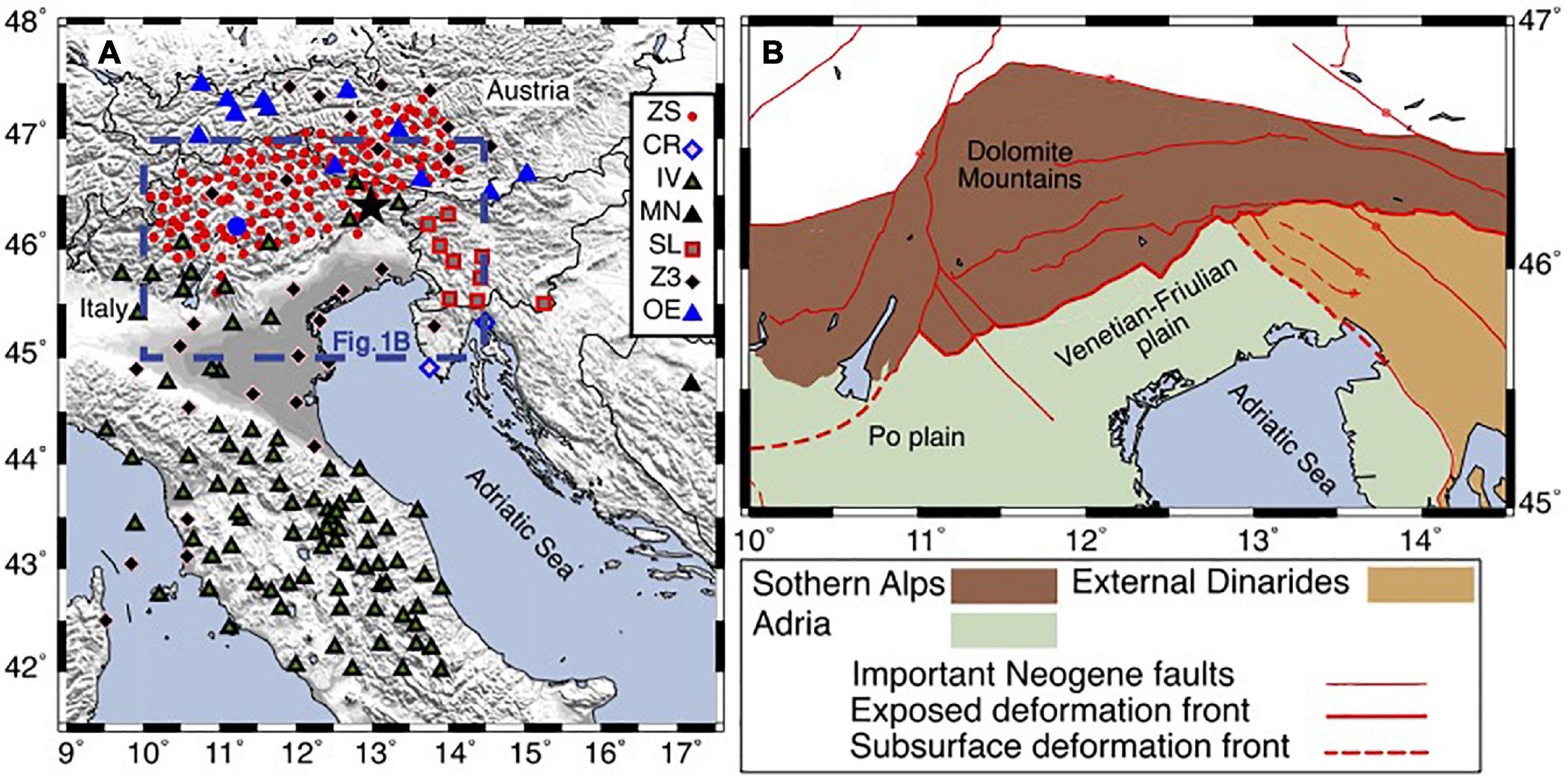
Figure 1. (A) Map showing the seismic stations used in this study. The ZS, CR, SL, and MN stations are used for computation of correlograms in this study. The correlograms computed using up to 4 years of the recordings from the IV, OE, and Z3 stations are adopted from Nouibat et al. (2021). The blue circle shows the location of D024 station of the ZS network and location of the June 14, 2019, Mw 3.7 earthquake is shown by black star. (B) Map showing the major tectonic features in the study region modified from Schmid et al. (2004, 2008) and Handy et al. (2010). ZS–SWATH-D temporary network; CR–Croatian seismograph network; IV–Italian national seismic network; MN–Mediterranean very broadband seismographic network; SL–Seismic network of the republic of Slovenia; Z3–AlpArray Z3 network; OE–Austrian seismic network.
We apply an ambient noise tomography to a new dataset exploiting the SWATH-D temporary experiment. Rayleigh wave phase velocity measurements obtained for pairs of stations are integrated with the measurements adopted from Nouibat et al. (2021). S-wave velocities are obtained by using non-perturbational and perturbational inversion in an area including the Friuli and Venetian plains, the Alps foothills, the Alpine chain and external Dinarides. A new high-resolution crustal model is computed down to a depth of 60 km and its relation with the main geologic and tectonic features are discussed. The estimated crustal thickness in the Southeastern Alps and external Dinarides is compared with those included in the Northern Adria crust (NAC) model (Magrin and Rossi, 2020) and the Moho map of Spada et al. (2013).
Data and Methods
Seismic Data and Cross Correlation
The dataset used in this study is composed of two subsets. The larger subset exploited 10 months of continuous recordings for computation of correlograms. The other smaller complementary subset of correlograms was adopted from Nouibat et al. (2021) (hereafter NBT21), which were calculated using up to 4 years of continuous recordings. Location of the seismic stations used in the two datasets is shown in Figure 1. In the following, we will present the description of these datasets.
The SWATH-D temporary experiment deployed 154 broadband seismic stations during 2017–2020. Taking the recording duration and quality of the stations into consideration, we processed 10 months of continuous seismic data recorded between October 2017 and July 2018 from 133 stations of the SWATH-D temporary network (ZS) (Heit et al., 2017). Continuous recordings of 13 permanent stations of the Slovenian (SL) (Slovenian Environment Agency, 2001), Croatian (CR) (University of Zagreb, 2001), and the Mediterranean very broadband (MN) (MedNet Project Partner Institutions, 1990) networks between October 2017 and July 2018 were also used (Figure 1).
The continuous data were baseline-corrected and downsampled to 5 Hz, and the instrumental response was removed. We followed the workflow proposed by Bensen et al. (2007) with slight modifications for the computation of cross-correlation of the vertical components. The waveforms were filtered between 0.5 and 100 s and cut to 1 h segments. We applied the time domain normalization and spectral whitening. We then cross-correlated the 1 h-long segments of all the ZS station pairs. We also performed the cross-correlation between the 1 h segments of the permanent stations (i.e., SL, CR, and MN networks) and all the ZS stations. Since the number of permanent station pairs is much smaller than the ZS-permanent station pairs and their ray crossings mainly coincide with those of the ZS-permanent and ZS-ZS station pairs, the cross-correlations between the permanent stations were not included. Subsequently, we stacked up to 24 available correlograms of each day. The resulting daily correlograms were stacked again over 3 months. We checked the quality of the correlograms by means of estimating the signal-to-noise-ratio (SNR). Then the SNR of the 3 month stacked correlograms were compared to investigate the seasonal variation in the quality of the correlograms. Comparison of the 3 month correlograms revealed that the correlograms were temporarily stable during the 10 month period of recording, and their SNR values did not exhibit substantial variations. Supplementary Figure S1 shows the 3 month correlograms with the SNR value of higher than 5 between station D024 (the blue circle in Figure 1) and other contemporaneously operating stations. We also stacked the daily correlograms for the 3–10 month periods to examine the effect of stacking duration on the quality of the correlograms. We fixed the value for the SNR threshold at 10. The results revealed that the SNR values of the majority of the station pairs were higher than the threshold after 7 months of stacking. Therefore, 10 months of stacking was sufficient to obtain stable correlograms (i.e., ZS, SL, MN, and CR station pairs).
At the end of this procedure, we selected 4050 high-quality empirical green functions (EGFs) showing clear and symmetrical signals on both the causal and acausal parts. Figure 2 shows the cross-correlations computed between station D024 (the blue circle in Figure 1) and other contemporaneously operating stations. Dispersive Rayleigh wave packets are evident on both the causal and acausal parts of the correlograms.
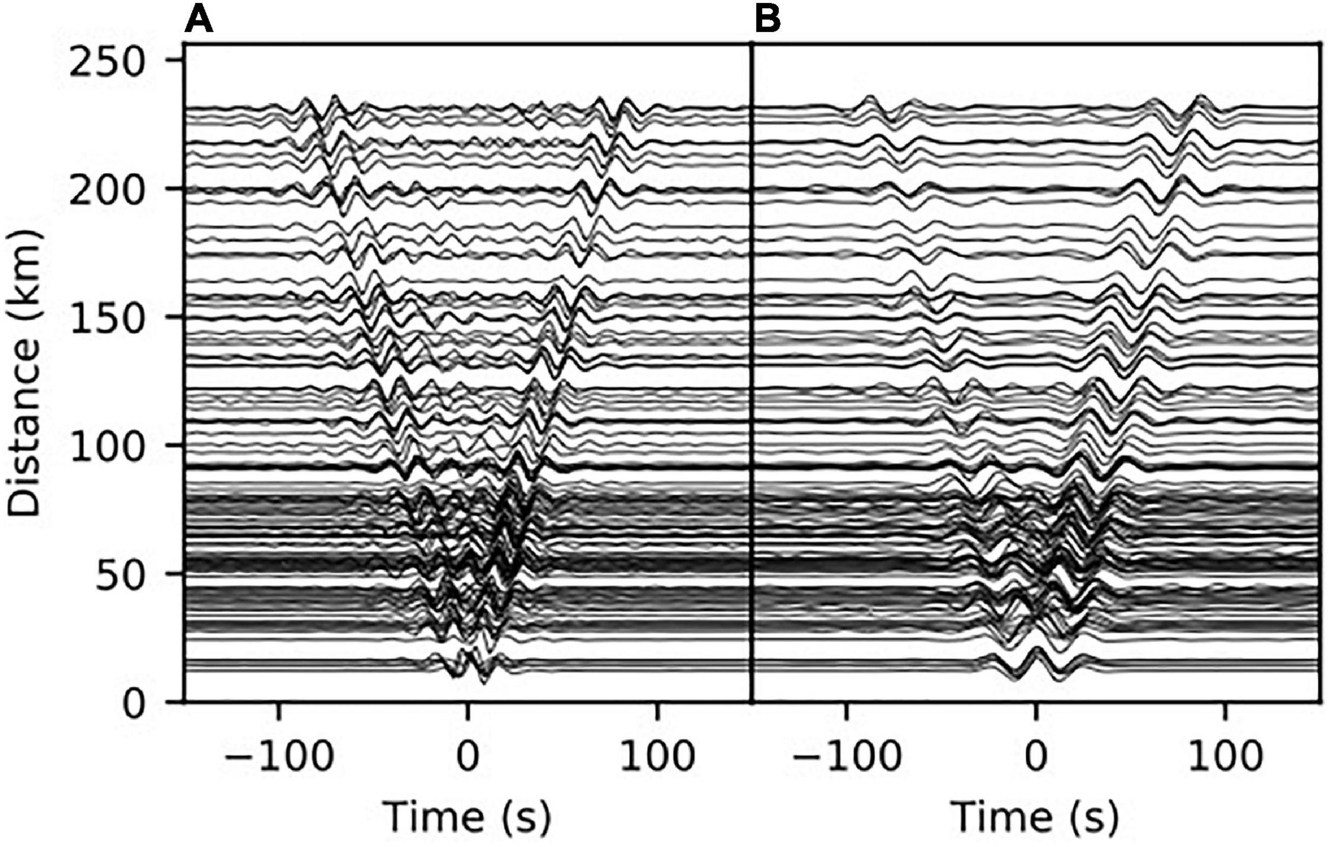
Figure 2. Examples of the stacked correlograms between station D024 (the blue circle in Figure 1) and other contemporaneously operating stations. Correlograms filtered in the period range of 10–20 s (A) and 20–40 s (B).
We followed the same procedure to compute the correlograms between some stations of the Italian national seismic network (IV) (INGV Seismological Data Centre, 1997) and the AlpArray Z3 network (Z3) (AlpArray Seismic Network, 2015) and the ZS stations to improve our ray coverage. However, unlike the ZS, SL, MN, and CR station pairs, the 10 month period of recording was not sufficient to satisfy our quality control criteria for the IV-Z3, IV-ZS, Z3-ZS station pairs. Therefore, we adopted 3036 correlograms from NBT21 as a complement to the dataset computed in this work. The correlograms were computed following the procedure explained in Soergel et al. (2020) and using up to 4 years of the continuous recordings of 148 stations of the IV, Austrian (OE) (Zentralanstalt Für Meterologie Und Geodynamik [ZAMG], 1987) and Z3 networks (Figure 1). Regardless of the time domain normalization, the preprocessing steps in the Soergel et al. (2020) procedure are mainly similar to the method we applied (i.e., detrending, low-pass filtering, and instrument response correction). This allows for the seamless integration of the correlograms computed in this study and those of NBT21. NBT21 followed the comb filter preprocessing routine for handling of transient high amplitude earthquake signals. They calculated the cross-correlations between each station pair using 4 h windows and stacked them to obtain the final correlogram for each station pair. We controlled the quality of the correlograms and kept 1804 EGFs with SNR values greater than 10 on both the causal and acausal parts to supplement our initial dataset. Figure 3 shows the variation in the number of EGFs with interstation distances and azimuths before and after inclusion of the high-quality correlograms of NBT21.
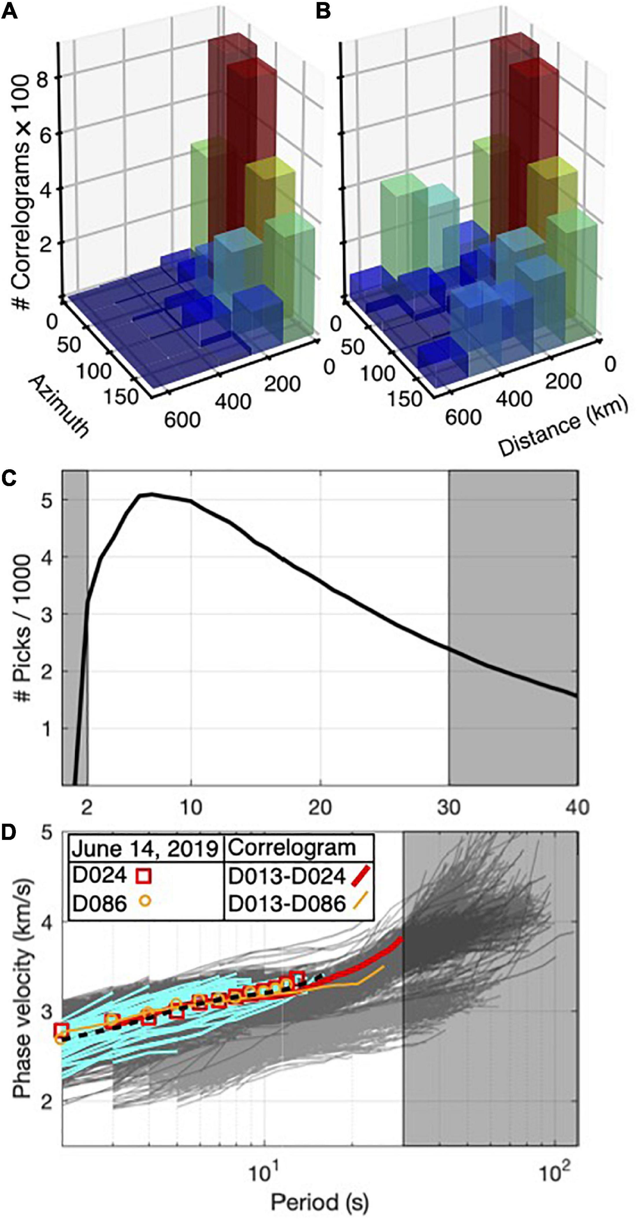
Figure 3. (A) Number of correlograms calculated in this study vs. interstation distance and azimuth. (B) Number of correlograms used in this study, including the high quality correlograms of Nouibat et al. (2021), vs. interstation distance and azimuth. (C) Number of Rayleigh phase velocity picks at different periods. (D) Phase velocity dispersion curves measured from correlograms calculated in this study (dark gray) superimposed on the dispersion curves measured from correlograms adopted from Nouibat et al. (2021) (lighter gray). The phase velocity dispersion curves from 44 records of the June 14, 2019, Mw 3.7 earthquake and the average curve are shown by cyan and black lines, respectively. The dispersion curves from D013-D024 and D013-D086 correlograms and those of the earthquake waveforms recorded by D024 and D086 stations are also shown. The horizontal axis label is shared in (C,D). Gray boxes in (C,D) show the periods excluded from tomography.
Rayleigh Wave Phase Velocity Measurements
The calculated EGFs have been then used to estimate the phase velocity of Rayleigh waves for each couple of stations. It is worth remembering that the largest period for which the phase velocity can be measured is proportional to the interstation distance. In the traditional frequency-time analysis (e.g., Levshin et al., 1992) the wavelength should be smaller than or equal to one-third of the interstation distance (Yao et al., 2006; Lin et al., 2008). However, the method of Ekström et al. (2009) allows for measuring reliable phase velocities up to periods with wavelength comparable to the interstation distance. The technique proposed by Ekström et al. (2009) uses the Aki’s spectral formulation to measure the phase velocity directly from the zero crossings of the real part of the correlation spectrum. We used the methodology of Ekström et al. (2009) incorporated into the GSpecDisp package (Sadeghisorkhani et al., 2017) for measuring the phase velocity dispersion curves of the Rayleigh waves. The reliable period range for each couple of stations was conservatively selected so that the interstation distance was 1.5–50 times larger than the considered wavelengths. We visually evaluated the causal and acausal parts of the EGFs and manually picked the dispersion curves exhibiting a clear, smooth and continuous trend of period dependence. The phase velocities were picked at periods where energy level on the real part of the correlogram spectrum is significant.
We also used the multiple-filter approach (Herrmann, 1973, 2013) to measure the phase velocities of some random correlograms and compared them with those obtained from GSpecDisp package. The comparison revealed no substantial difference between the dispersion curves in the period range where 3–50 wavelengths can propagate within the interstation distance. Furthermore, we measured the phase velocities from 44 records of June 14, 2019, Mw 3.7 earthquake (the black star in Figure 1) using the multiple-filter approach (Herrmann, 1973, 2013) to further validate the dispersion curves obtained from correlograms. The earthquake epicenter is located close to station D013 of the ZS network. The dispersion curves from June 14, 2019, Mw 3.7 earthquake were in agreement with those from correlograms between D013 and other ZS stations (Figure 3). Figure 3D shows the dispersion curves picked from the D013-D024 and D013-D086 correlograms as well as the dispersion curves from the waveforms of June 14, 2019, Mw 3.7 earthquake recorded by D024 (46.21°N, 11.23°E) and D086 (46.64°N, 11.35°E) stations. At periods longer than 30 s, the dispersion curves obtained from the correlogram dataset of NBT21 exhibit two diverging trends. The set of dispersion curves with lower velocities at longer periods are related to the rays crossing the Po and Venetian-Friuli plains, while the dispersion curves of the rays crossing the Alps have higher velocities at periods longer than 30 s.
Figure 3C shows the number of phase velocities obtained from correlograms in the period range of 2–30 s. The number of measurements varies between 2,390 in 30 s and 5,094 in 7 s. Since the SNR of most of the 3 month stacked correlograms were smaller than the threshold of 10 we were not able to estimate the uncertainty of the phase velocity measurements from seasonal variability as it is proposed by Bensen et al. (2007).
2D Phase Velocity Tomography
The fast-marching surface wave tomography package (FMST) (Rawlinson, 2005) is used for inversion of the reliable Rayleigh wave phase velocity measurements. FMST uses the fast-marching method (Sethian and Popovici, 1999) for the forward prediction of the traveltimes. It applies an iterative subspace inversion to map lateral variations in phase velocity accounting for the non-linear relationship between velocity and traveltime. The study area was parameterized with 0.1° × 0.1°cell grids. The cell grid size is selected so that each cell in the target region contains a minimum of 20 ray crossings. The average of the measured phase velocities at each period was considered as the homogeneous starting model of the inversion. FMST allows the damping and smoothing regularization parameters to be adjusted in order to cope with the problem of non-uniqueness. The damping factor prevents the solution model from departing too much from the starting model, while the smoothing factor avoids unrealistic sudden changes and constrains the smoothness of the solution model. Although the dispersion curves were picked carefully, we first ran the inversions with a high value of damping factor to detect and discard the highly incoherent paths with the traveltime residual greater than three times the average of all the traveltime residuals (Kaviani et al., 2020). We performed the tomographic inversion again with a set of regularization parameter pairs in the range between 0 and 5 to select the optimal damping and smoothing parameters at each period. The optimal damping and smoothing parameters were selected by the construction of the trade-off curves. After careful inspection of the trade-off between data misfit and model variance at each period, the damping factor was chosen. The trade-off curves between misfit and model roughness were used to estimate the optimal smoothing parameters at each period. Figure 4 shows the smoothing and damping trade-off curves and the selected optimal parameters for periods of 5 and 20 s.
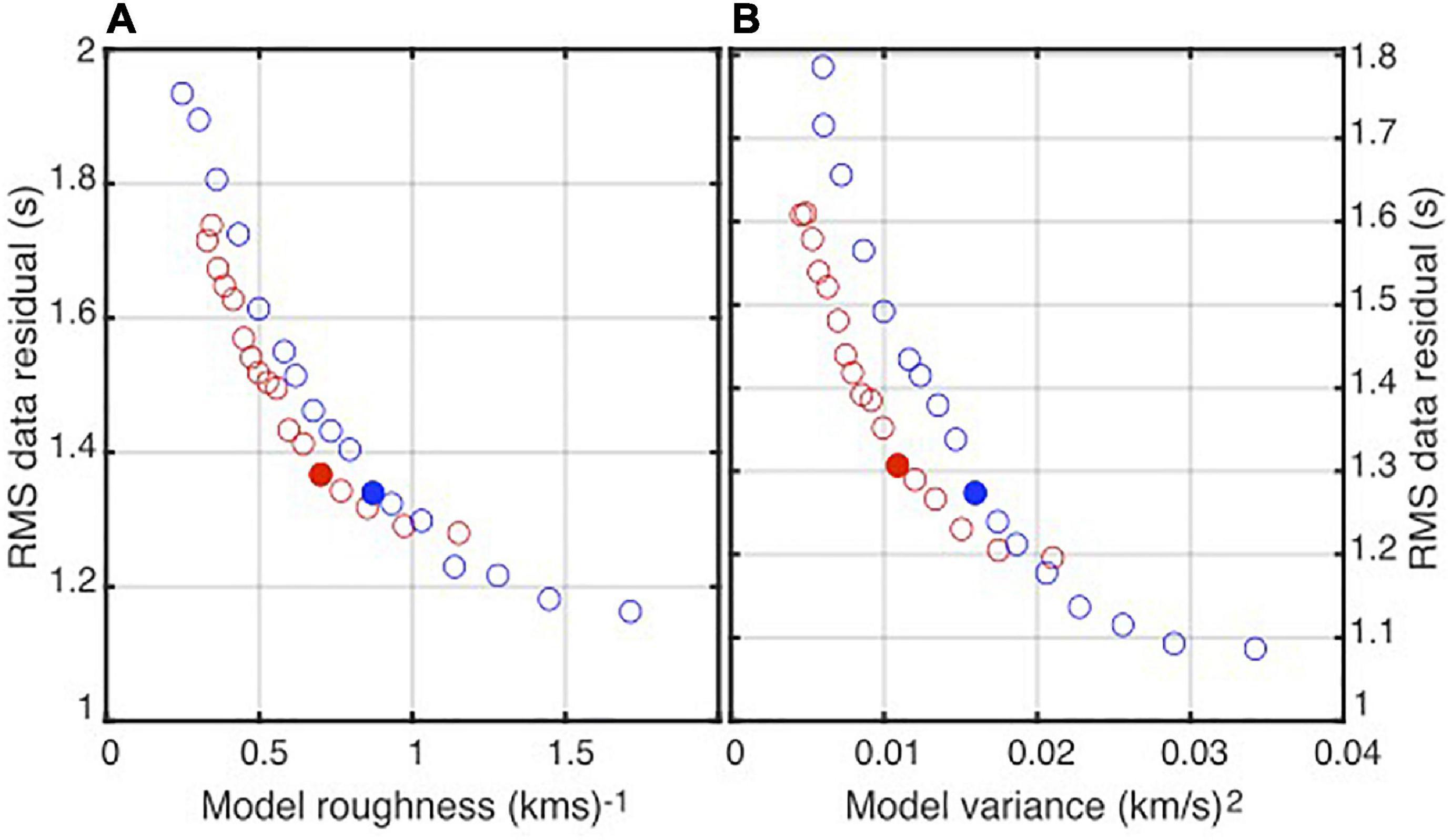
Figure 4. The trade-off curves between misfit and model roughness for different smoothing parameters (A) and the trade-off curves between misfit and model variance for different damping parameters (B) for periods of 5 s (red) and 20 s (blue). Damping and smoothing parameters change in the range between 0 and 5. The selected optimal smoothing and damping parameters are shown by filled circles.
We performed checkerboard tests to elucidate the dimensions of the features that can be resolved through the inversion process. The actual ray coverage and the selected optimal regularization parameters were used in the checkerboard tests. Thanks to the dense ray coverage, the 0.3° × 0.3° blocks at periods shorter than 5 s were recovered in the Southeastern Alps region covered by the ZS network. However, smearing effects are obvious at periods longer than 4 s. Performing the checkerboard tests with anomaly sizes of 0.5° × 0.5° revealed that the anomalies are well recovered in most of the target region (Figure 5).
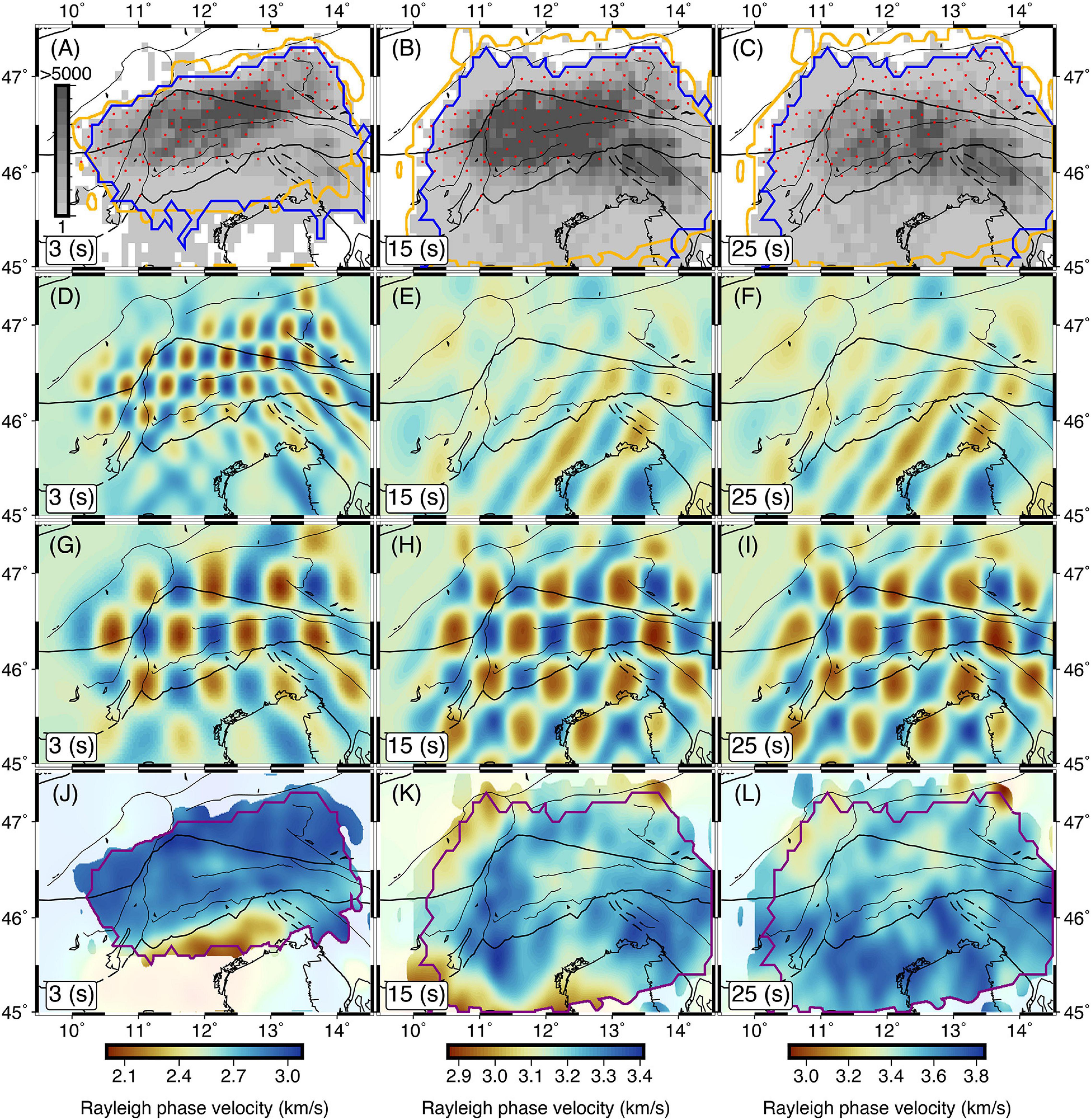
Figure 5. Number of ray crossings in each 0.1° × 0.1° grid cell and stations of the ZS network (A–C). The area with resolvability factor of higher than 0.7 and the tomographic grids with minimum of 20 ray crossings are shown by orange and blue polygons, respectively. Checkerboard reconstruction results with anomaly size of 0.3° × 0.3° (D–F) and 0.5° × 0.5° (G–I), and tomographic inversion results at periods of 3, 15, and 25 s (J–L). The purple polygon illustrates the overlapped area between the resolvability factor higher than 0.7 and the minimum of 20 ray crossings.
Following Zelt (1998), we quantitatively assessed the semblance between the true and recovered checkerboard anomalies through the calculation of the resolvability factor. The areas in tomographic results with resolvability factor of higher than 0.7, and the tomographic grids with a minimum of 20 ray crossings are shown in Figure 5. The final tomographic results are confined within the overlapped area between the resolvability factor of higher than 0.7 and a minimum of 20 ray crossings (Figure 5). We initially performed the tomography for the period range between 2 and 40 s. However, considering the checkerboard test results, we decided to confine the final tomographic inversions to the 2–30 s period band in the region covered by ZS network and to the 5–30 s period range in the remaining parts.
1D S-wave Velocity Inversion
We extracted local dispersion curves for each 0.1° × 0.1° grid node of the tomographic model and inverted them for 1D depth-dependent S-wave velocity profiles. We performed the two-step procedure of Haney and Tsai (2017) for non-perturbational and perturbational inversion of Rayleigh-wave velocities. First, we applied the non-perturbational inversion, based on the Dix-type relation for surface waves, and an optimal non-uniform finite-element grid of layers generated based on depth sensitivity of the Rayleigh waves (Haney and Tsai, 2015; Figure 6). The 1D velocity profiles obtained were then used as starting models for the subsequent perturbational inversion that relies on the finite-element method resulting in a matrix formulation of the forward problem. It allows for linking the forward and inverse problems using matrix perturbation theory. The perturbational inversion iteratively refines the starting model provided by the non-perturbational Dix-type inversion to find the final model that fits the data. We generated a set of synthetic phase velocity dispersion curves with 2.5% noise from arbitrary velocity models. A comparison of the inverted and true models revealed that the inversion process is capable of producing a smoothed version of the true model (Supplementary Figure S2).
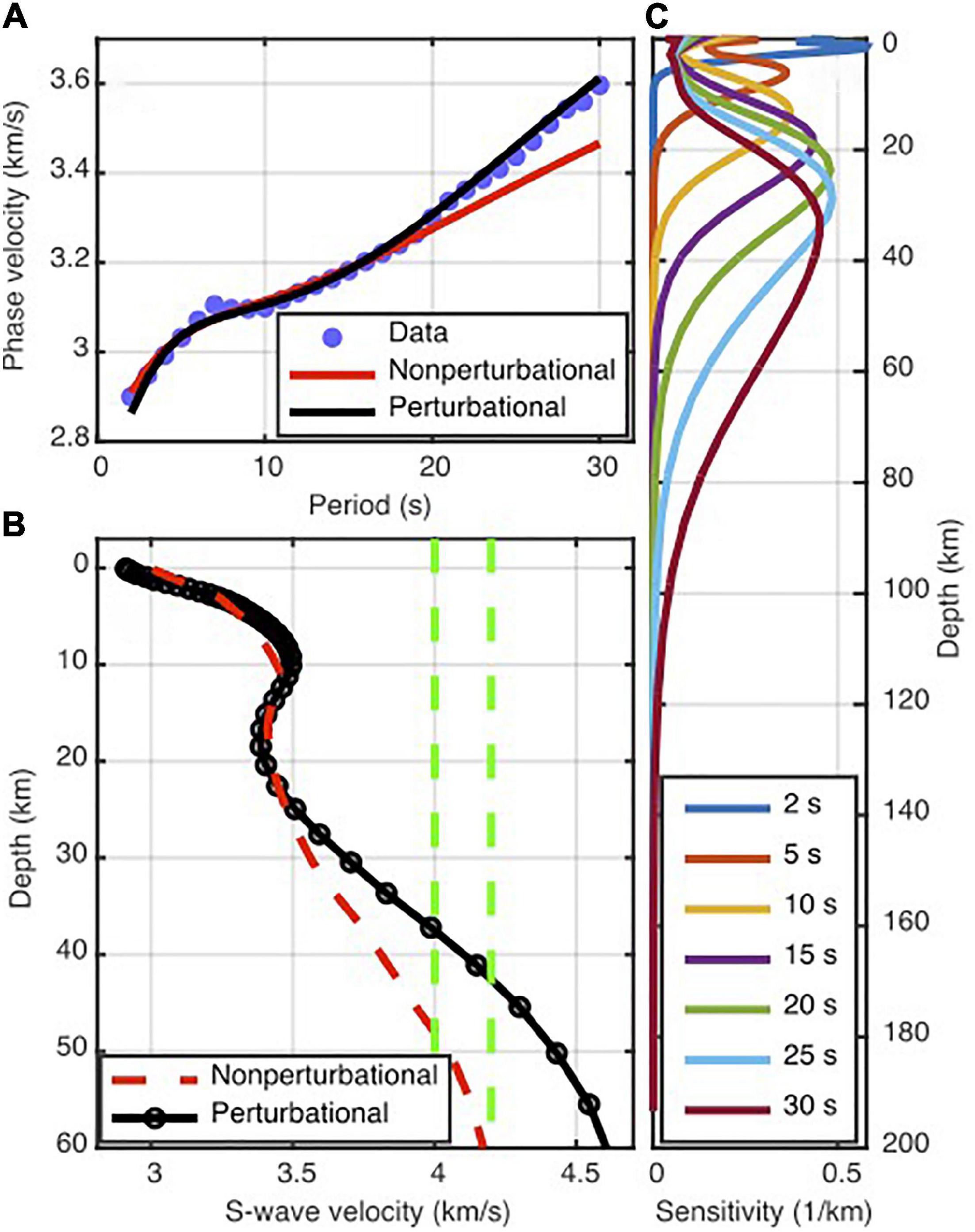
Figure 6. (A) An example local dispersion curve and predicted curves from non-perturbational (initial model) and perturbational (final model) inversions. (B) Inverted S-wave velocity depth models using non-perturbational (initial model) and perturbational (final model) inversions. Black circles represent the optimal non-uniform finite-element grid of layers. S-wave velocities of 4.0 and 4.2 km/s as candidate velocities for detecting the Moho at depth are shown by vertical green dashed lines. (C) Sensitivity kernel of the final perturbational model.
Figure 6 shows an example of the measured and predicted dispersion curves as well as the starting and final S-wave velocity models at a grid node. Although the perturbational updating of the non-perturbational starting model has not substantially affected the shallower S-wave velocity structures, it leads to significant fitting improvements at longer period dispersions representing the deeper S-wave velocity structures. We inverted the local dispersion curves for the 1D velocity profiles down to a depth of more than 200 km. However, considering the sensitivity kernels calculated using the final S-wave velocity model, we consider as reliable the results obtained down to 60 km (Figure 6). Four examples of the inverted 1D S-wave velocity profiles and their sensitivity kernels are shown in Supplementary Figure S3.
Results
3D S-wave Velocity Model
After inverting all the local dispersion curves, we assembled the resulting 1D S-wave velocity profiles into a pseudo-3D crustal S-wave velocity model of the Southeastern Alps (hereafter SEA-Crust). Figure 7A shows seven depth slices from the surface down to 60 km. The average velocity is increasing from about 2.0 km/s at the surface to about 4.5 km/s at the depth of 60 km. The average 1D S-wave velocity profiles of the Alps and the Friuli and Venetian plains are shown in Figure 7B. The P-wave velocities in Figure 7B were calculated considering the average crustal Poisson ratio of 0.256 (Christensen, 1996). In the depths shallower than about 15 km and to the north of the deformation front, S-wave velocity is higher than the southern parts (i.e., in the Venetian and Friuli plains). In contrast, deeper depth slices reveal higher velocities in the Venetian and Friuli plains compared to the Eastern Alps. Considering both the S-wave velocities of 4.0 and 4.2 km/s as proxies for the Moho depth, the crust in the eastern Alps is, on average, about 15 km thicker than in the Venetian and Friuli plains (Figure 7). At 60 km depth, the depth slice is dominated by velocities greater than 4.0 km, implying that the crust in the whole study region should not be thicker than 60 km.
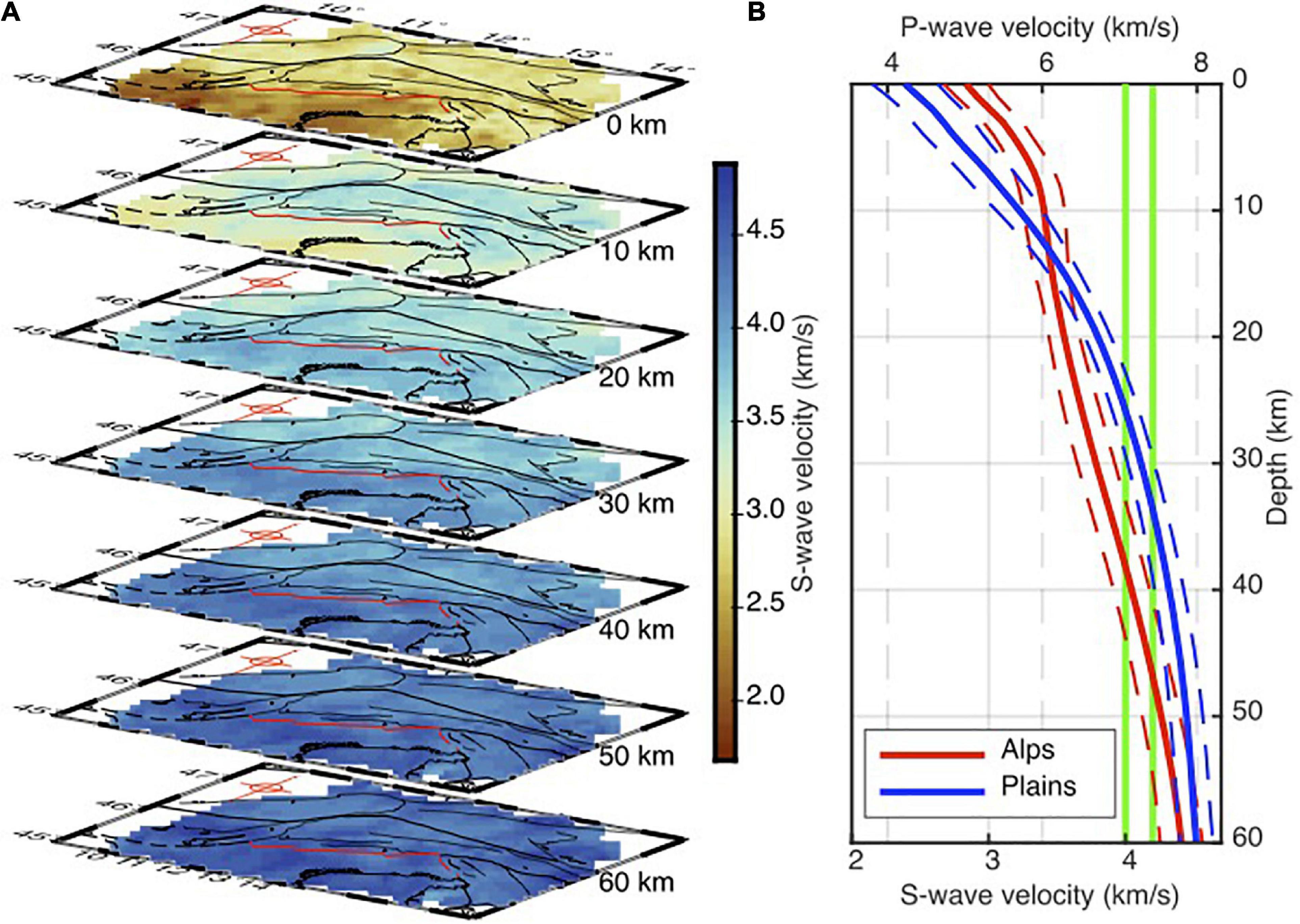
Figure 7. (A) Depth slices showing variation of the S-wave velocity from the surface down to 60 km depth. The border between the Southeastern Alps and the Venetian and Friuli plains is shown by the red line. The thinner black lines depict the Neogene faults (Schmid et al., 2004, 2008; Handy et al., 2010). (B) The average 1D S-wave velocity profiles in the Southeastern Alps and the Venetian and Friuli plains. S-wave velocities of 4.0 and 4.2 km/s are shown by vertical green lines. The P-wave velocity profiles are calculated considering the average Poisson ratio of 0.256 for the continental crust (Christensen, 1996).
Figures 8A–H shows the variation of S-wave velocity with respect to the average velocity at different depths from 5 to 40 km. Figure 8I shows the major faults in the region. The absolute velocities at the same depths are shown in Supplementary Figure S4. The Southern prominent low-velocity zone at 5 and 10 km depths is related to the Venetian and Friuli plains. The upper crustal S-wave velocities change considerably from the Friuli and Venetian plains to the Alps foothills. As we expected, in the shallow crust, the S-wave velocities are lower for the Adria plate beneath the Friuli and Venetian plains, where soft sediments and sedimentary rocks are thicker. The S-wave velocity at 10 km depth in the Southeastern Alps reaches the value of about 3.8 km/s that is in agreement with the high P-wave velocity value of 6.8 km/s reported by other works (Behm, 2009; Bressan et al., 2012). Considering the increasing trend of the crustal thickness from the south to the north of the study region, the 15–30 and 20–40 km depth ranges are approximately associated with the middle-lower crust in the Southeastern Alps and Adria, respectively. The maps of absolute velocity in Supplementary Figure S4 reveal that the middle and lower crust are faster in the southern parts than in the northern parts of the study region. Nonetheless, a more rigid lower and middle crust for the Adria plate is not a new result and is consistent with the efficient wave propagation due to low attenuation of recorded earthquakes and SmS wave propagation (e.g., Bragato et al., 2011; Sugan and Vuan, 2014). The faster middle and lower crust of the Adria compared to the Southeastern Alps is also observed by the other recent tomographies (Kästle et al., 2018; Lu et al., 2018; Qorbani et al., 2020).
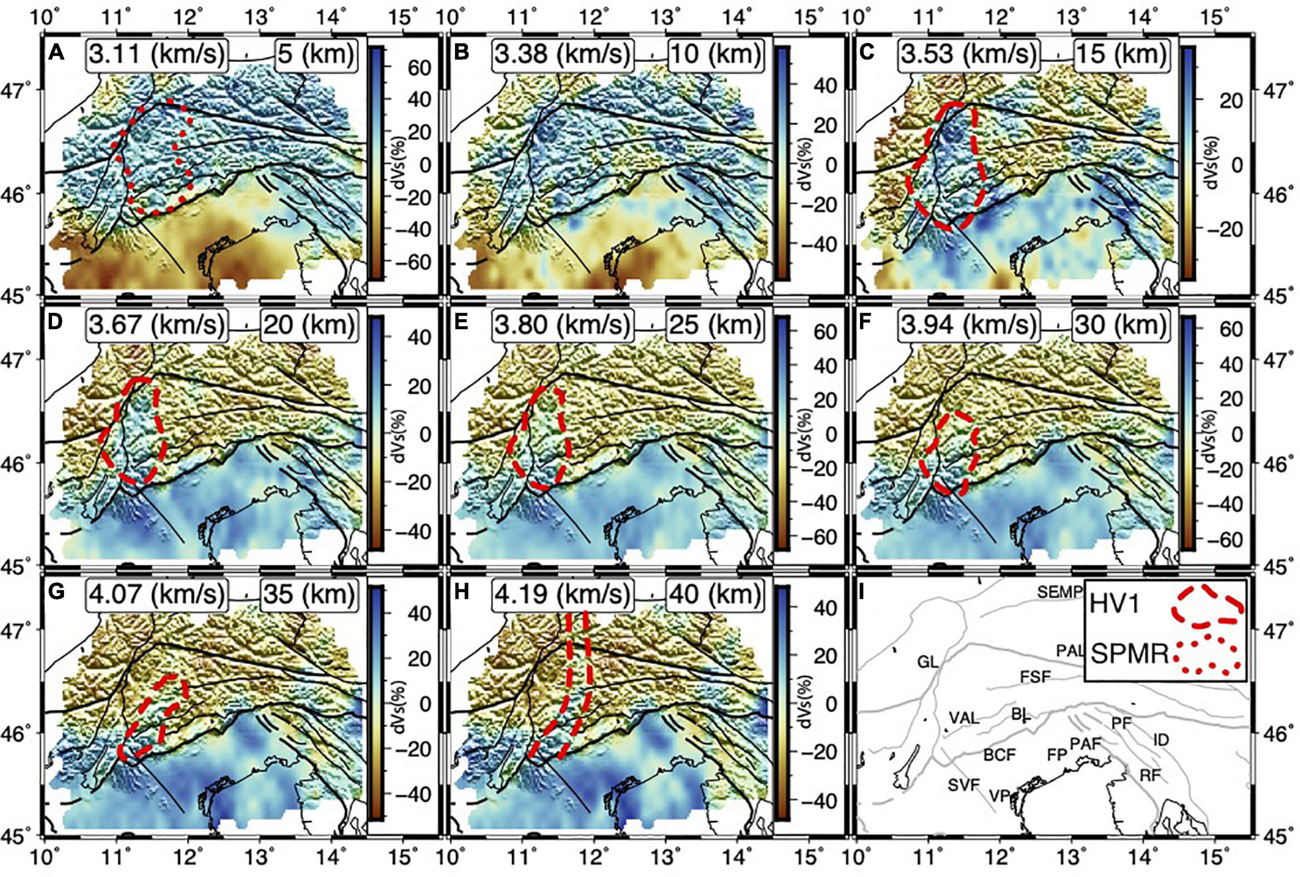
Figure 8. Depth slices showing the S-wave velocity anomalies at 5, 10, 15, 20, 25, 30, 35, and 40 km (A–H). The average S-wave velocity is shown in each panel. Location of the Permian magmatic rocks observed at the surface is shown in (A). (I) Map showing the major faults in the region. SPMR, Surface Permian magmatic rocks.
The boundary between the higher and lower velocity anomalies to the east of longitude 12°E and in the 15–40 km depth range perfectly mimics the leading edge of the Alpine front responsible for the 1976 Friuli earthquake (Aoudia et al., 2000) to the east and the Bassano-Cansiglio active folding system to the west (Figure 8). The presence of a high-velocity body (HV1) deeper than 10 km to the east of the Giudicarie fault is evident. The NNW oriented part of HV1 at 40 km depth is also clearly observed by Molinari et al. (2020) and roughly observed by Kästle et al. (2018) and Lu et al. (2018). On the other hand, such a high-velocity body seems to be absent from both the Love and Rayleigh-wave shear velocity model of Qorbani et al. (2020). The location of the HV1 at 10–20 km depth range coincides with the Permian magmatic rocks at the surface (Schuster and Stüwe, 2008). The eastward extension of HV1 with depth can be considered as the continuation of the Permian magmatic complex within the lower crust. The low-velocity anomaly in the 10–20 km depth range and to the northwest of the study region is also observed by Qorbani et al. (2020).
Crystalline Basement and Moho Depth
Different criteria have been used by receiver function and tomography studies to capture the sedimentary layer-crystalline basement boundary and the Moho discontinuity. Using the iso-velocities at the bottom of the layers is among the most well-established approaches for estimation of the discontinuity depths in seismic imaging studies. However, the S-wave iso-velocities used in the literature range from 1.5 to 3.0 km/s and from 3.9 to 4.3 km/s for depicting the basement and Moho depths, respectively (Christensen and Mooney, 1995; Brocher, 2005; Moschetti et al., 2010; Molinari and Morelli, 2011; Macquet et al., 2014; An et al., 2015; Guidarelli et al., 2017; Magrin and Rossi, 2020; Planès et al., 2020). Part of this discrepancy originates from the lack of single definitions of the discontinuities and the trade-off between the S-wave velocity and the depth of the discontinuities. If the S-wave velocities of both the top and the bottom layers are estimated, a strong depth gradient of the 1D S-wave velocity profile can be considered as an indicator of the discontinuity.
We used the gradient of the 1D velocity profiles in the top 10 km as a proxy to select the reasonable iso-velocity representing the crystalline basement depth. Figure 9A presents the number of maximum depth gradients in various velocities. Considering the histogram, we selected the average depths corresponding to a range of velocities between 2.8 and 3.0 km/s as the indicator of the discontinuity. A map illustrating the crystalline basement depth is presented in Figure 9B. It shows that the crystalline basement depths in the Po, Venetian and Friuli plains ranges between ∼4 and ∼10 km. In the same region, Qorbani et al. (2020) has also traced a low-velocity anomaly with values of less than 3.0 km/s down the 10 km.
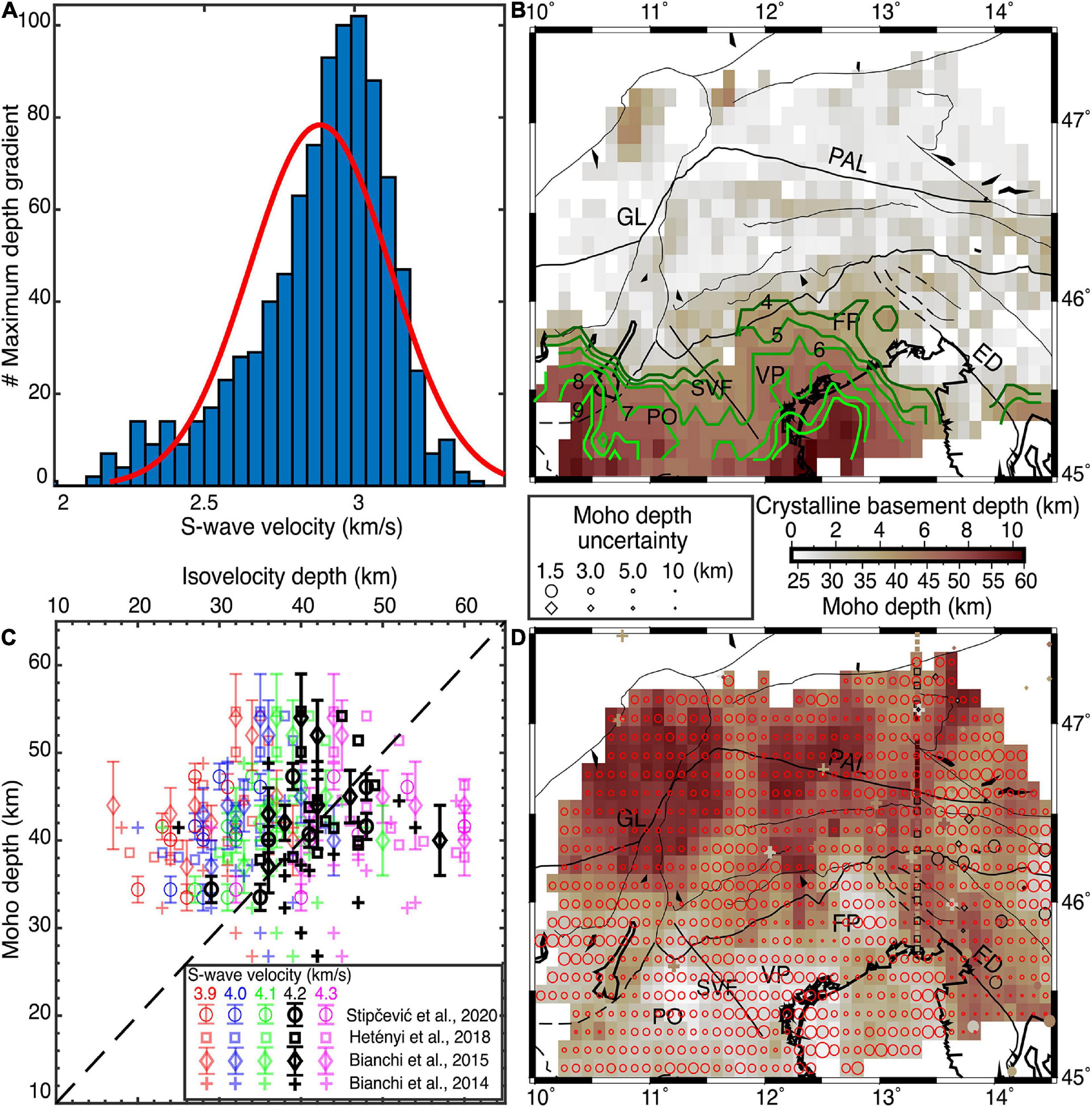
Figure 9. (A) A histogram showing the variation in the number of maximum depth gradients of the 1D S-wave velocity profiles with S-wave velocity. The best fitting normal distribution is shown by red. (B) The crystalline basement depth estimated by the average of iso-velocity depths between 2.8 and 3.0 km/s. Green lines portray the basement depth contours from 4 km (darkest green) to 9 km (lightest green). (C) Comparison between receiver function Moho depths and the depths obtained from iso-velocities ranging from 3.9 to 4.3 km/s. The horizontal axis label is shown on the top axis. (D) Moho depth estimated by the average of iso-velocity depths between 4.1 and 4.3 km/s. The Moho depths adopted from receiver function studies are shown by the same symbols as in (C) and their sizes are proportional to their uncertainty (if it was available). The receiver function depths used for the comparison in (C) are marked by black outline. The size of the red circles represents the uncertainty of the Moho at each node. PAL, Periadriatic Line; SVF, Schio-Vicenza fault; GL, Giudicarie Line; FP, Friuli Plain; VP, Venetian Plain; PO, Po Plain; ED, External Dinarides.
According to Steinhart (1967) and Thybo et al. (2013), the seismic Moho is defined as a rapid increase of the crustal P-wave velocity to a value in the range of 7.6 and 8.6 km/s. In the absence of a sharp increase in velocity, the Moho is the level at which the P-wave velocity exceeds the 7.6 km/s threshold. Taking the average crustal Poisson ratio of 0.256 (Christensen, 1996) into account, the S-wave threshold velocity is 4.3 km (An et al., 2015). In some part of the study region (i.e., beneath the Southeastern Alps) the Moho is deeper than 55 km which is close to the maximum depth of SEA-Crust (Molinari and Morelli, 2011; Spada et al., 2013; Bianchi and Bokelmann, 2014; Bianchi et al., 2015; Hetényi et al., 2018b; Kästle et al., 2018; Lu et al., 2018, 2020; Stipčević et al., 2020). Therefore, in these regions, SEA-Crust is not able to sample the shallow uppermost mantle beneath such a deep Moho and the 1D velocity models vary smoothly with depth, especially toward the deepest parts. Thus, for estimating the crustal thickness we preferred to use the iso-velocity depths rather than depth gradient of the 1D velocity profiles. To this end, we collected a set of available Moho depths from receiver function studies (Bianchi et al., 2014, 2015; Hetényi et al., 2018b; Stipčević et al., 2020) and compared them with different depths of iso-velocities between 3.9 and 4.3 km/s. Figure 9C illustrates the receiver function Moho depths vs. iso-velocity depths. The comparison revealed that the 4.2 km/s iso-velocity depths are in a general agreement with the receiver function results. The 4.1 and 4.3 km/s iso-velocities mainly give rise to underestimation and overestimation of the Moho depth, respectively. However, considering the available uncertainty of the receiver function results, some of the 4.1 and 4.3 km/s iso-velocity depths are acceptable. Thus, the average of the iso-velocity depths between 4.1 and 4.3 km/s is taken to be the Moho depth. We calculated the standard deviation of the depths in the same iso-velocity range as a measure of uncertainty of the Moho depth (Figure 9D). The general pattern of higher uncertainties for the deeper Moho depth estimates is partly due to the decreasing vertical resolution with depth.
Discussion
Comparison of the Pseudo-3D S-wave Model With Other Studies
We compared SEA-Crust with those of NAC (Magrin and Rossi, 2020) and Kästle et al. (2018) (hereafter KST18) through the calculation of their relative changes (Supplementary Figures S5–S7) for fixed-depth slices. Mapping the local differences in the upper crust (5 and 10 km depth, Supplementary Figure S5), NAC is faster than SEA-Crust almost everywhere in the Po and Venetian-Friuli plains (more than 20% at 5 km depth). Beneath the southernmost SWATH-D development and at 5 and 10 km depths, the relative change between SEA-Crust and NAC is smaller (∼10%) (Supplementary Figure S5). This consistency between SEA-Crust and NAC coincides with the region where NAC is constrained by local earthquake tomographies (Anselmi et al., 2011; Bressan et al., 2012; Viganò et al., 2013). Within the 20–30 km depth range, NAC is, on average, faster (less than 10%) than SEA-Crust beneath the Alps and slower beneath the plains (Supplementary Figure S5). NAC also tends to be slower than SEA-Crust (less than 15%) in the lower crust (depth >30 km) and almost everywhere in the study region (Supplementary Figure S5).
In the upper crust (depth <10 km), SEA-Crust appears to be on average ∼10% faster and slower than KST18 in the Southeastern Alps and in the plains, respectively (Supplementary Figure S6). Within the 20–30 km depth range, KST18 is ∼10% slower than SEA-Crust (Supplementary Figure S6). The S-wave velocity differences between KST18 and SEA-Crust increase gradually with depth and reach ∼15% at 35 km. Toward the deeper structures and between 50 and 60 km depths, while the KST18 is slower than SEA-Crust (less than 10%) beneath the plains, it turns out to be faster (less than 10%) beneath the Alps (Supplementary Figure S6).
Extremely variable S-wave velocities characterize the plains, which is also pronounced by differences between NAC and KST18 (Supplementary Figure S7). Comparing the three models shows that SEA-Crust in the upper crust is more compatible with KST18 rather than NAC all around the study region. This is probably as a result of the similarities between the approaches used by this study and KST18.
A peculiarity of SEA-Crust is that it exploited the new dataset of phase velocities extracted from the SWATH-D station pairs with short interstation distances. Therefore, we expect SEA-Crust to be more selective and accurate for the paths crossing the plains and the Alpine region at short periods and shallower depths. It can justify the higher relative changes in SEA-Crust with respect to NAC and KST18 in the shallow crust (Supplementary Figures S5, S6).
Border of the Po and Venetian-Friuli Plains
The Southern low-velocity anomaly at 5 km in Figure 8A coincides with the location of the well-known Po, Venetian and Friuli plains. The S-wave velocity in the region covered by the basins is not homogeneous, and a relatively higher velocity trend beneath the Schio-Vicenza fault divides it into the eastern and western lower velocity parts. The S-wave velocity range between 2.8 and 3.0 km/s used for determination of the basement depth is in the same range as those reported for the Mesozoic carbonates on top of the crystalline basement (Pola et al., 2014; Turrini et al., 2014; Molinari et al., 2020). The estimated basement depth in Figure 9B is in turn shallower (∼5 km) beneath the Schio-Vicenza fault compared to its western and eastern deepest parts (∼10 km) to the southwest of the Garda Lake and the northwestern corner of the Adriatic Sea. The topography of the crystalline basement depth correlates well with the depth of the Pliocene base related to the softer sediments (Pola et al., 2014). The N-S cross sections in Figure 10 also highlight the soft and consolidated sedimentary cover of the Venetian and Friuli plains that is negatively correlated to the topography.
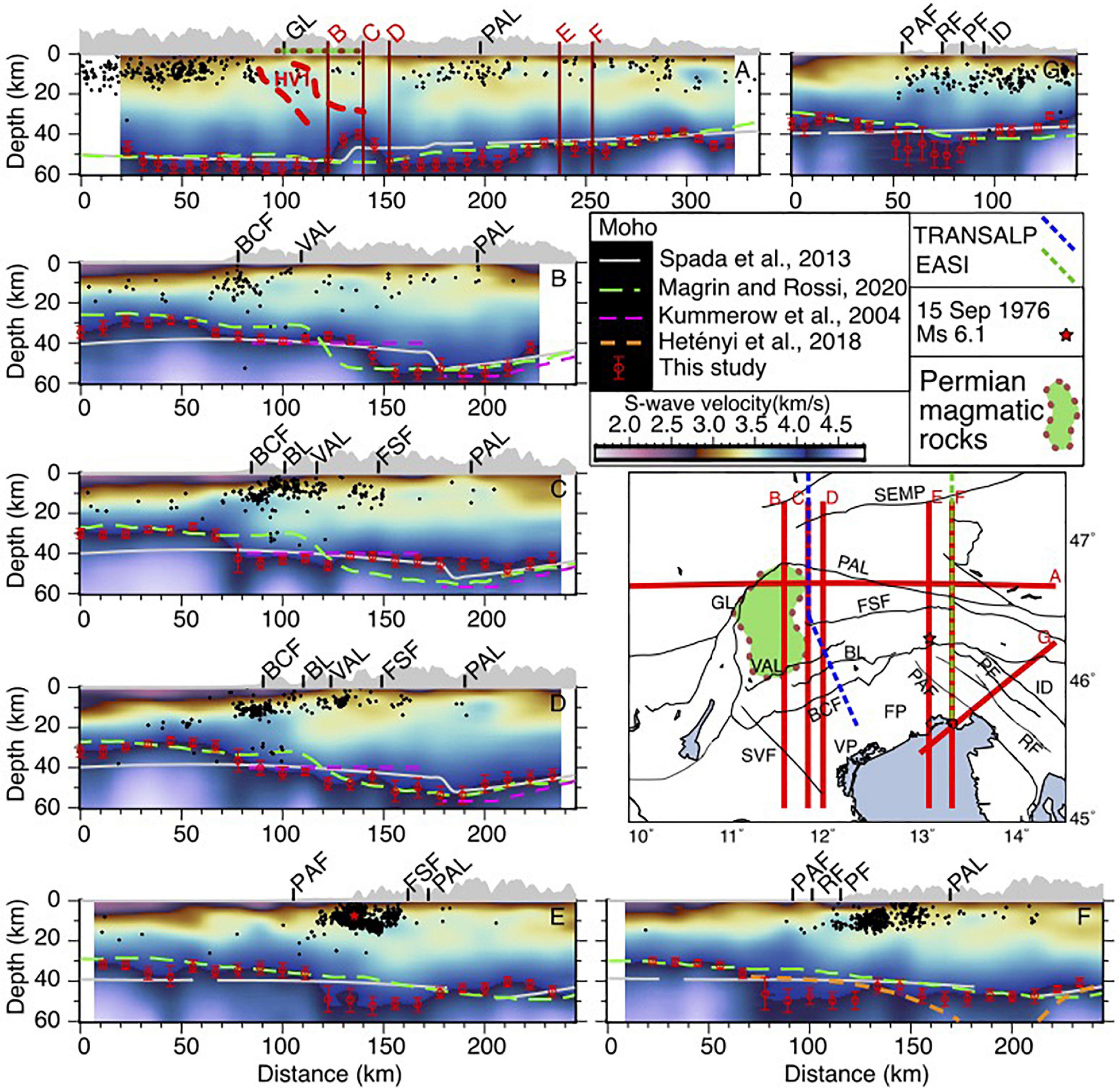
Figure 10. Cross sections of the S-wave velocity model. The seismic events within 0.05° from the profiles are extracted from the OGS catalog (Friuli-Venezia Giulia Seismometric Network Bulletin, 2019) and projected along the sections. PAL, Periadriatic Line; GL, Giudicarie Line; FP, Friuli Plain; VP, Venetian Plain; SEMP, Salzach-Ennstal-Mariazell-Puchberg; VAL, Valsugana thrust; BL, Belluno Line; FSF, Fella-Sava Fault; ID, Idrija Fault; BCF, Bassano-Cansiglio Fault; PAF, Palmanova fault; RA, Rasa fault; PF, Predjama Fault.
Upper and Middle Crustal Structure vs. Seismicity
The N-S cross sections in Figure 10 reveal that the middle and lower crust, particularly toward the northern parts is highly heterogeneous. Part of this heterogeneity comes from a vertical sequence of higher and lower velocity layers beneath the Southeastern Alps, which is also detectable in section A. Beneath the Adria plate, there are sharp velocity transitions between the upper, middle and the lower crust; the middle crust seems to be well developed with velocity gradients. However, toward the north, the velocity gradients are laterally distorted by high-velocity bodies in the upper and middle crust starting from the foothills of the Alps. The seismicity we plotted along the cross sections spans from 2008 to 2019 and are extracted from the OGS catalog (Friuli-Venezia Giulia Seismometric Network Bulletin, 2019). The seismicity is mainly located in the southern front of the Alps (i.e., where the elevation increases along the topographic sections) and is confined in a narrow velocity band between ∼3.1 and ∼3.6 km/s (Figure 10). The 15 September 1976 (Ms = 6.1) earthquake (Aoudia et al., 2000) is shown in section E, and its adjacent seismicity clearly reveals the concentration of the seismicity on the interface separating the higher velocity from the lower velocity zones. The concentration of the seismic activity in the narrow velocity band is also in agreement with the occurrence of large earthquakes in the upper-crustal density domain boundaries and the regions of the highest geodetic strain rate (Spooner et al., 2019). This supports the hypothesis that the faster middle and lower crust of Adria in this area is more rigid than the Southeastern Alps, while the faster upper crust of southeastern Alps is more rigid than Adria (e.g., Brückl et al., 2007, 2010; Marotta and Splendore, 2014; Magrin and Rossi, 2020).
Moho Topography
During the last two decades, important efforts were made to determine the crustal thickness of the Alps through different approaches (e.g., Kummerow et al., 2004; Spada et al., 2013; Hetényi et al., 2018b; Kästle et al., 2018; Lu et al., 2018, 2020; Spooner et al., 2019; Magrin and Rossi, 2020). The Moho model of Spada et al. (2013) is derived from a combination of receiver function and controlled source seismological studies. The more recently published study of Magrin and Rossi (2020) is focused on the northern tip of the Adria plate (i.e., about the same study area as ours). They integrated the available information about the depth of the main interfaces and the physical properties of the crust to build the NAC model. The continuous Moho map of NAC and the crustal thickness model of Spada et al. (2013) are plotted along all the sections in Figure 10.
Figure 9D shows the crustal thickness map from the average depths between 4.1 and 4.3 km/s iso-velocities. The red circles in Figure 9D represent the location of the estimation nodes, and their size are inversely proportional to the uncertainty of the estimates. Crustal thickening, as expected, is found in our results from south to north (Figures 9D, 10). Taking the uncertainties into account, while the thinner crust of the Adria plate is shown as gentle undulations that seems to be consistent with NAC, the Moho model of Spada et al. (2013) is about 10 km deeper (see sections B, D, and C in Figure 10). Moving toward the north and along the sections B, C, and D, the change in our Moho depth at the Alps foothills is sharper than the other models, and the crustal thickness mirrors the topography, particularly in section D (Figure 10). The Moho depth of Kummerow et al. (2004) beneath the TRANSALP profile is depicted in sections B, C, and D.
Surprisingly, considering the three adjacent sections, it appears that the maximum Moho depth beneath the Dolomite Mountains significantly varies from more than 50 km in section B and D to ∼40 km in section C which coincides with the location of TRANSALP. In section B, a sharp Moho step with magnitude of more than 15 km is positioned between the Moho gradients in the NAC and Spada et al. (2013) models. In section C, by contrast, the Moho depth remains unchanged at ∼40 km toward the north of the Alps foothills. While the magnitude of crustal thickness in section D is similar to section B, the Moho depth increases at a longer wavelength along the profile in section D. Section A, perpendicular to the three adjacent sections, clearly portrays the N-S narrow corridor of crustal thinning. The shallower Moho in section C is located beneath the surface observation of the Permian magmatic rocks and HV1 that can be considered as the continuation of the Permian magmatism to the deep-seated crust. Presence of a much smoother lateral variation in the crustal thickness to the east of the Giudicarie line is reported by Kästle et al. (2018) and Spooner et al. (2019).
Except for the inconsistencies in their middle parts, the Moho depths in sections E, F, and G generally agree with the NAC Moho. The deeper Moho to the north of the Palmanova fault is consistent with the results of the recent receiver function study of Stipčević et al. (2020). The NW-SE thickened crust along the boundary between the Friuli plain and the external Dinarides is mainly formed as a result of the past and ongoing Adria-Europe convergence, which is accommodated by thrusting and strike slip faulting (Vičič et al., 2019). The crustal thickness from the receiver functions of Hetényi et al. (2018b) along the EASI profile is shown in section F. The EASI Moho beneath the Periadriatic Line reaches the depths of more than 60 km, which is far deeper than the values of the other models. The southern part of the EASI crosses the thickened crust to the east of the Friuli plain (∼50 km). However, the thick crust in this region is not captured by EASI receiver functions (Hetényi et al., 2018b) and it shows a ∼10 km thinner crust which is consistent with Spada et al. (2013) and slightly deeper than the NAC Moho.
Conclusion
We compiled a collection of 5854 correlograms calculated using the continuous seismic recordings from the permanent and temporary networks in Italy, Austria, Slovenia and Croatia. Most of the correlograms are computed using the seismic recordings of the AlpArray SWATH-D complementary experiment, and additional 1084 EGFs are provided by Nouibat et al. (2021). We used the GSpecDisp package (Sadeghisorkhani et al., 2017) for measuring the phase velocity dispersion curves of the Rayleigh waves between 2 and 30 s. The FMST package is applied for the Rayleigh phase velocity tomography in a 0.1° × 0.1° grid covering the Southeastern Alps, the western part of the external Dinarides, and the Friuli and Venetian plains. We inverted the resulting local dispersion curves for 1D S-wave velocity profiles using the non-perturbational and perturbational inversion methods (Haney and Tsai, 2015, 2017). Finally, the 1D S-wave velocity profiles are assembled into a pseudo-3D S-wave velocity model. By using the depth gradient of the 1D S-wave velocity profiles, the depth of the crystalline basement beneath each node is determined. We also compared the iso-velocity depths with the crustal thickness inferred from receiver functions and found the 4.2 km/s iso-velocity to be a reasonable representation of the Moho depth. Taking the resulted S-wave velocity model and the crystalline basement and Moho depth maps into account, the following principal conclusions can be drawn:
- Thanks to the close station spacing of the SWATH-D network, our S-wave velocity model contains more details compared to the other available models (e.g., Kästle et al., 2018; Magrin and Rossi, 2020) particularly at shallower depths.
- The crystalline basement depth in the Po, Venetian and Friuli plains, ranges between ∼4 and ∼10 km.
- The crystalline basement beneath the Schio-Vicenza fault is shallower (∼5 km) than its eastern and western regions implying that the Schio-Vicenza fault can be considered as a prominent structural feature between the Venetian and Friuli plains to the east and the Po-plain to the west.
- Comparison of the shallow crustal velocities and location of the earthquakes in the southern foothills of the Alps reveals that the seismicity mainly occurs in a narrow velocity band between ∼3.1 and ∼3.6 km/s.
- The map of the iso-velocity-based Moho depth illustrates a N-S trending narrow corridor of thinner crust (∼40 km) beneath the Dolomite Mountains and along the TRANSALP profile, which separates the eastern and western thicker (∼55 km) crustal cores.
- The Moho depth map displays a thickened crust along the boundary between the Friuli Plain and the external Dinarides.
Data Availability Statement
The raw data supporting the conclusions of this article including the pseudo-3D crustal S-wave velocity model, and the Moho and basement depths of the Southeastern Alps, the western part of the external Dinarides, and the Friuli and Venetian plains (SEA-Crust) are publicly accessible at: https://doi.org/10.5281/zenodo.4574022.
Author Contributions
AS-B: conceptualization, data curation, methodology, software, writing original draft, writing, review and editing and visualization. AV: data curation, conceptualization, methodology, software, writing original draft, writing, review and editing, visualization, funding acquisition, and supervision. AA: methodology, writing original draft, writing, review and editing, validation, funding acquisition, and supervision. SP: validation, writing review and editing, funding acquisition and Supervision. AlpArray and AlpArray-Swath-D Working Group: design of experiment, data acquisition, data curation, funding acquisition. All authors contributed to the article and approved the submitted version.
Conflict of Interest
The authors declare that the research was conducted in the absence of any commercial or financial relationships that could be construed as a potential conflict of interest.
Acknowledgments
The maps are plotted using perceptually uniform colormaps (Crameri, 2018). AS-B acknowledges support from the ICTP TRIL (Training and Research in Italian Laboratories) programme (ICTP-OGS agreement). We thank the editor, GH, and the reviewers, IM, and IB, for their constructive comments. We thank Ahmed Nouibat and Anne Paul for sharing part of their correlogram dataset and Nick Rawlinson for the FMST tomography code. We appreciate helpful discussions with Andrea Magrin and Giuliana Rossi. The equipment for the SWATH-D array was provided by the Geophysical Instrument Pool Potsdam (GIPP of the GFZ grant number 201717) (https://www.gfz-potsdam.de/gipp) and DSEBRA (http://www.spp-mountainbuilding.de/research/project_reports/DSEBRA_2018.pdf). We acknowledge the AlpArray-Swath D Working Group: B. Heit, M. Weber, C. Haberland, F. Tilmann, the AlpArray-Swath D Field Team: Luigia Cristiano (Freie Universität Berlin, Helmholtz-Zentrum Potsdam Deutsches GeoForschungsZentrum (GFZ), Peter Pilz, Camilla Cattania, Francesco Maccaferri, Angelo Strollo, Günter Asch, Peter Wigger, James Mechie, Karl Otto, Patricia Ritter, Djamil Al-Halbouni, Alexandra Mauerberger, Ariane Siebert, Leonard Grabow, Susanne Hemmleb, Xiaohui Yuan, Thomas Zieke, Martin Haxter, Karl-Heinz Jaeckel, Christoph Sens-Schonfelder (GFZ), Michael Weber, Ludwig Kuhn, Florian Dorgerloh, Stefan Mauerberger, Jan Seidemann (Universität Potsdam), Frederik Tilmann, Rens Hofman (Freie Universität Berlin), Yan Jia, Nikolaus Horn, Helmut Hausmann, Stefan Weginger, Anton Vogelmann [Austria: Zentralanstalt für Meteorologie und Geodynamik (ZAMG)], Claudio Carraro, Corrado Morelli (Südtirol/Bozen: Amt für Geologie und Baustoffprüfung), Günther Walcher, Martin Pernter, Markus Rauch (Civil Protection Bozen), Damiano Pesaresi, Giorgio Duri, Michele Bertoni, Paolo Fabris [Istituto Nazionale di Oceanografia e di Geofisica Sperimentale OGS (CRS Udine)], Andrea Franceschini, Mauro Zambotto, Luca Froner, Marco Garbin (also OGS) (Ufficio Studi Sismici e Geotecnici -Trento) and the institutions that provided permanent station data in the AlpArray Project. We would like to thank to the AlpArray Seismic Network Team: GH, Rafael Abreu, Ivo Allegretti, Maria-Theresia Apoloner, Coralie Aubert, Simon Besançon, Maxime Bès de berc, Götz Bokelmann, Didier Brunel, Marco Capello, Martina Čarman, Adriano Cavaliere, Jérôme Chèze, Claudio Chiarabba, John Clinton, Glenn Cougoulat, Wayne C. Crawford, Luigia Cristiano, Tibor Czifra, Ezio D’alema, Stefania Danesi, Romuald Daniel, Anke Dannowski, Iva Dasović, Anne Deschamps, Jean-Xavier Dessa, Cécile Doubre, Sven Egdorf, ETHZ-SED Electronics Lab, Tomislav Fiket, Kasper Fischer, Wolfgang Friederich, Florian Fuchs, Sigward Funke, Domenico Giardini, Aladino Govoni, Zoltán Gráczer, Gidera Gröschl, Stefan Heimers, Ben Heit, Davorka Herak, Marijan Herak, Johann Huber, Dejan Jarić, Petr Jedlička, Yan Jia, Hélène Jund, Edi Kissling, Stefan Klingen, Bernhard Klotz, Petr Kolínský, Heidrun Kopp, Michael Korn, Josef Kotek, Lothar Kühne, Krešo Kuk, Dietrich Lange, Jürgen Loos, Sara Lovati, Deny Malengros, Lucia Margheriti, Christophe Maron, Xavier Martin, Marco Massa, Francesco Mazzarini, Thomas Meier, Laurent Métral, IM, Milena Moretti, Anna Nardi, Jurij Pahor, Anne Paul, Catherine Péquegnat, Daniel Petersen, Damiano Pesaresi, Davide Piccinini, Claudia Piromallo, Thomas Plenefisch, Jaroslava Plomerová, Silvia Pondrelli, Snježan Prevolnik, Roman Racine, Marc Régnier, Miriam Reiss, Joachim Ritter, Georg Rümpker, Simone Salimbeni, Marco Santulin, Werner Scherer, Sven Schippkus, Detlef Schulte-Kortnack, Vesna Šipka, Stefano Solarino, Daniele Spallarossa, Kathrin Spieker, Josip Stipčević, Angelo Strollo, Bálint Süle, Gyöngyvér Szanyi, Eszter Szűcs, Christine Thomas, Martin Thorwart, Frederik Tilmann, Stefan Ueding, Massimiliano Vallocchia, Luděk Vecsey, René Voigt, Joachim Wassermann, Zoltán Wéber, Christian Weidle, Viktor Wesztergom, Gauthier Weyland, Stefan Wiemer, Felix Wolf, David Wolyniec, Thomas Zieke, Mladen Živčić, and Helena Žlebčíková.
Supplementary Material
The Supplementary Material for this article can be found online at: https://www.frontiersin.org/articles/10.3389/feart.2021.641113/full#supplementary-material and doi: 10.5281/zenodo.4574022
Supplementary Figure 1 | Three month correlograms with the SNR value of higher than 5 between station D024 (the blue circle in Figure 1) and other contemporaneously operating stations.
Supplementary Figure 2 | Synthetic 1D velocity inversion tests. The True and the inverted models are shown by cyan and red, respectively.
Supplementary Figure 3 | Four examples of the inverted 1D S-wave velocity profiles and their sensitivity kernels. Locations of the 1D profiles are mentioned in the panels.
Supplementary Figure 4 | Depth slices showing the absolute S-wave velocity values at 5, 10, 15, 20, 25, 30, 35, and 40 km. Location of the Permian magmatic rocks observed at the surface is shown in (A). SPMR–Surface Permian magmatic rocks.
Supplementary Figure 5 | Depth slices showing the relative change in the S-wave velocities of SEA-Crust (this study) with respect to NAC (Magrin and Rossi, 2020). The relative change is calculated as [(SEA-Crust–NAC)/NAC]. FP, Friuli Plain; VP, Venetian Plain; PO, Po Plain.
Supplementary Figure 6 | Depth slices showing the relative change in the S-wave velocities of SEA-Crust (this study) with respect to KST18 (Kästle et al., 2018). The relative change is calculated as [(SEA-Crust–KST18)/KST18]. FP, Friuli Plain; VP, Venetian Plain; PO, Po Plain.
Supplementary Figure 7 | Depth slices showing the relative change in the S-wave velocities of NAC (Magrin and Rossi, 2020) with respect to KST18 (Kästle et al., 2018). The relative change is calculated as [(NAC-KST18)/KST18]. FP, Friuli Plain; VP, Venetian Plain; PO, Po Plain.
References
AlpArray Seismic Network (2015). AlpArray Seismic Network (AASN) Temporary Component. AlpArray Working Group. Other/Seismic Network. International Federation of Digital Seismograph Networks. doi: 10.12686/alparray/z3_2015
An, M., Wiens, D. A., Zhao, Y., Feng, M., Nyblade, A. A., Kanao, M., et al. (2015). S-velocity model and inferred Moho topography beneath the Antarctic Plate from Rayleigh waves. J. Geophys. Res. Solid Earth 120, 359–383. doi: 10.1002/2014jb011332
Anselmi, M., Govoni, A., De Gori, P., and Chiarabba, C. (2011). Seismicity and velocity structures along the South-Alpine thrust front of the Venetian Alps (NE-Italy). Tectonophysics 513, 37–48. doi: 10.1016/j.tecto.2011.09.023
Aoudia, A., SaraoÌ, A., Bukchin, B., and Suhadolc, P. (2000). The 1976 Friuli (NE Italy) thrust faulting earthquake: a reappraisal 23 years later. Geophys. Res. Lett. 27, 577–580. doi: 10.1029/1999GL011071
Behm, M. (2009). 3-D modelling of the crustal S-wave velocity structure from active source data: application to the Eastern Alps and the Bohemian Massif. Geophys. J. Int. 179, 265–278. doi: 10.1111/j.1365-246X.2009.04259.x
Behm, M., Nakata, N., and Bokelmann, G. (2016). Regional ambient noise tomography in the Eastern Alps of Europe. Pure Appl. Geophys. 173, 2813–2840. doi: 10.1007/s00024-016-1314-z
Bensen, G. D., Ritzwoller, M. H., Barmin, M. P., Levshin, A. L., Lin, F., Moschetti, M. P., et al. (2007). Processing seismic ambient noise data to obtain reliable broad-band surface wave dispersion measurements. Geophys. J. Int. 169, 1239–1260. doi: 10.1111/j.1365-246X.2007.03374.x
Bianchi, I., Behm, M., Rumpfhuber, E. M., and Bokelmann, G. (2015). A new seismic data set on the depth of the Moho in the Alps. Pure Appl. Geophys. 172, 295–308. doi: 10.1007/s00024-014-0953-1
Bianchi, I., and Bokelmann, G. (2014). Seismic signature of the Alpine indentation, evidence from the Eastern Alps. J. Geodyn. 82, 69–77. doi: 10.1016/j.jog.2014.07.005
Bianchi, I., Miller, M. S., and Bokelmann, G. (2014). Insights on the upper mantle beneath the Eastern Alps. Earth Planet. Sci. Lett. 403, 199–209. doi: 10.1016/j.epsl.2014.06.051
Bianchi, I., Ruigrok, E., Obermann, A., and Kissling, E. (2020). Moho Topography Beneath the Eastern European Alps by Global Phase Seismic Interferometry, Solid Earth Discuss. [Preprint]. In review. doi: 10.5194/se-2020-179
Bragato, P. L., Sugan, M., Augliera, P., Massa, M., Vuan, A., and Saraò, A. (2011). Moho reflection effects in the Po plain (northern Italy) observed from instrumental and intensity data. Bull. Seismol. Soc. Am. 101, 2142–2152. doi: 10.1785/0120100257
Bressan, G., Gentile, G. F., Tondi, R., de Franco, R., and Urban, S. (2012). Sequential integrated inversion of tomographic images and gravity data: an application to the Friuli area (North-Eastern Italy). Boll. Geof. Teor. Appl. 53, 191–212. doi: 10.4430/bgta0059
Bressan, G., Ponton, M., Rossi, G., and Urban, S. (2016). Spatial organization of seismicity and fracture pattern in NE-Italy and W-Slovenia. J. Seismol. 20, 511–534. doi: 10.1007/s10950-015-9541-9
Brocher, T. (2005). Empirical relations between elastic wavespeeds and density in the Earth’s crust. Bull. Seismol. Soc. Am. 95, 2081–2092. doi: 10.1785/0120050077
Brückl, E., Behm, M., Decker, K., Grad, M., Guterch, A., Keller, G. R., et al. (2010). Crustal structure and active tectonics in the Eastern Alps. Tectonics 29:TC2011. doi: 10.1029/2009TC002491
Brückl, E., Bleibinhaus, F., Gosar, A., Grad, M., Guterch, A., Hrubcovaì, P., et al. (2007). Crustal structure due to collisional and escape tectonics in the Eastern Alps region based on profiles Alp01 and Alp02 from the ALP 2002 seismic experiment. J. Geophys. Res. Solid Earth. 112:B06308.
Christensen, N., and Mooney, W. D. (1995). Seismic velocity structure and composition of the continental crust: a global view. J. Geophys. Res. 100, 9761–9788. doi: 10.1029/95JB00259
Christensen, N. I. (1996). Poisson’s ratio and crustal seismology. J. Geophys. Res. 101, 3139–3156. doi: 10.1029/95JB03446
Dewey, J. F., Helman, M. L., Knott, S. D., Turco, E., and Hutton, D. H. W. (1989). Kinematics of the western mediterranean. Geol. Soc. Lond. Spec. Publ. 45, 265–283. doi: 10.1144/gsl.sp.1989.045.01.15
Ekström, G., Abers, G. A., and Webb, S. C. (2009). Determination of surface-wave phase velocities across US array from noise and Aki’s spectral formulation. Geophys. Res. Lett. 36:L18301. doi: 10.1029/2009GL039131
Finetti, I. R. (ed.) (2005). CROP Project: Deep Seismic Exploration of the Central Mediterranean, and Italy, Vol. 1. Amsterdam: Elsevier.
Friuli-Venezia Giulia Seismometric Network Bulletin (2019). Available online at: http://www.crs.inogs.it/bollettino/RSFVG/RSFVG.en.html (accessed September 22, 2020).
Grad, M., Brückl, E., Majdan ìski, M., Behm, M., Guterch, A., and CELEBRATION 2000 and ALP 2002 Working Groups (2009). Crustal structure of the Eastern Alps and their foreland: seismic model beneath the CEL10/Alp04 profile and tectonic implications. Geophys. J. Int. 177, 279–295. doi: 10.1111/j.1365-246x.2008.04074.x
Guidarelli, M., Aoudia, A., and Costa, G. (2017). 3-D structure of the crust and uppermost mantle at the junction between the southeastern Alps and external dinarides from ambient noise tomography. Geophys. J. Int. 211, 1509–1523. doi: 10.1093/gji/ggx379
Handy, M. R., Schmid, S. M., Bousquet, R., Kissling, E., and Bernoulli, D. (2010). Reconciling plate-tectonic reconstructions of Alpine Tethys with the geological-geophysical record of spreading and subduction in the Alps. Earth Sci. Rev. 102, 121–158. doi: 10.1016/j.earscirev.2010.06.002
Handy, M. R., Ustaszewski, K., and Kissling, E. (2015). Reconstructing the Alps-carpathians-dinarides as a key to understand switches in subduction polarity, slab gaps and surface motion. Int. J. Earth Sci. 104, 1–26. doi: 10.1007/s00531-014-1060-3
Haney, M. M., and Tsai, V. C. (2015). Nonperturbational surface-wave inver- sion: a dix-type relation for surface waves. Geophysics 80, EN167–EN177. doi: 10.1190/geo2014-0612.1
Haney, M. M., and Tsai, V. C. (2017). Perturbational and nonperturbational in- version of Rayleigh-wave velocities. Geophysics 82, F15–F28. doi: 10.1190/GEO2016-0397.1
Heit, B., Weber, M., Tilmann, F., Haberland, C., Jia, Y., Carraro, C., et al. (2017). The Swath-D Seismic Network in Italy and Austria. GFZ Data Services. Other/Seismic Network. doi: 10.14470/mf7562601148
Herrmann, R. B. (1973). Some aspects of band-pass filtering of surface waves. Bull. Seismol. Soc. Am. 63, 663–671.
Herrmann, R. B. (2013). Computer programs in seismology: an evolving tool for instruction and research, Seism. Res. Lettr. 84, 1081–1088. doi: 10.1785/0220110096
Hetényi, G., Molinari, I., Clinton, J., Bokelmann, G., Bondár, I., Crawford, W. C., et al. (2018a). The AlpArray seismic network: a large-scale European experiment to image the Alpine orogeny, Surv. Geophy. 39, 1009–1033. doi: 10.1007/s10712-018-9472-4
Hetényi, G., Plomerová, J., Bianchi, I., Kampfová Exnerová, H., Bokelmann, G., Handy, M. R., et al. (2018b). From mountain summits to roots: crustal structure of the Eastern Alps and bohemian massif along longitude 13.3°E. Tectonophysics 744, 239–255. doi: 10.1016/j.tecto.2018.07.001
INGV Seismological Data Centre (1997). Rete Sismica Nazionale (RSN). Italy: Istituto Nazionale di Geofisica e Vulcanologia [INGV], doi: 10.13127/SD/X0FXnH7QfY
Istituto Nazionale Di Oceanografia E Di Geofisica Sperimentale (2016). North-East Italy Seismic Network. International Federation of Digital Seismograph Networks. Sgonico: Istituto Nazionale Di Oceanografia E Di Geofisica Sperimentale, doi: 10.7914/SN/OX
Kästle, E. D., El-Sharkawy, A., Boschi, L., Meier, T., Rosenberg, C., Bellahsen, N., et al. (2018). Surface wave tomography of the Alps using ambient-noise and earthquake phase velocity measurements. J. Geophys. Res. 123, 1770–1792. doi: 10.1002/2017JB014698
Kaviani, A., Paul, A., Moradi, A., Mai, P. M., Pilia, S., Boschi, L., et al. (2020). Crustal and uppermost mantle shear wave velocity structure beneath the Middle East from surface wave tomography. Geophys. J. Int. 221, 1349–1365. doi: 10.1093/gji/ggaa075
Kissling, E., Schmid, S. M., Lippitsch, R., Ansorge, J., and Fügenschuh, B. (2006). “Lithosphere structure and tectonic evolution of the Alpine arc: new evidence from high- resolution teleseismic tomography,” in European Lithosphere Dynamics, eds D. G. Gee and R. A. Stephenson (London: Geological Society Memoir), 3229–3145.
Kummerow, J., Kind, R., Oncken, O., Giese, P., Ryberg, T., Wylegalla, K., et al. (2004). A natural and controlled source seismic profile through the Eastern Alps: TRANSALP. Earth Planet. Sci. Lett. 225, 115–129. doi: 10.1016/j.epsl.2004.05.040
Kvapil, J., Plomerová, J., Kampfová Exnerová, H., Babuška, V., Hetényi, G., and The AlpArray Working Group (2020). Transversely Isotropic Lower Crust of Variscan Central Europe imaged by Ambient Noise Tomography of the Bohemian Massif, Solid Earth Discuss. [Preprint]. In review. doi: 10.5194/se-2020-176.
Le Breton, E., Handy, M. R., Molli, G., and Ustaszewski, K. (2017). Post-20 Ma motion of the Adriatic plate: New constraints from surrounding Orogens and implications for crust-mantle decoupling. Tectonics 36, 3135–3154. doi: 10.1002/2016TC004443
Levshin, A., Ratnikova, L., and Berger, J. (1992). Peculiarities of surface-wave propagation across central Eurasia. Bull. Seismol. Soc. Am. 82, 2464–2493.
Lin, F. C., Moschetti, M. P., and Ritzwoller, M. H. (2008). Surface wave tomography of the western United States from ambient seismic noise: rayleigh and love wave phase velocity maps. Geophys. J. Int. 173, 281–298. doi: 10.1111/j.1365-246X.2008.03720.x
Lu, Y., Stehly, L., Brossier, R., Paul, A., and AlpArray Working Group (2020). Imaging Alpine crust using ambient noise wave-equation tomography. Geophys. J. Int. 222, 69–85. doi: 10.1093/gji/ggaa145
Lu, Y., Stehly, L., Paul, A., and AlpArray Working Group (2018). High-resolution surface wave tomography of the European crust and uppermost mantle from ambient seismic noise. Geophys. J. Int. 214, 1136–1150. doi: 10.1093/gji/ggy188
Macquet, M., Paul, A., Pedersen, H. A., Villasen or, A., Chevrot, S., Sylvander, M., et al. (2014). Ambient noise tomography of the pyrenees and the surrounding regions: inversion for a 3-D vs model in the presence of a very heterogeneous crust. J. Geophys. Int. 199, 402–415. doi: 10.1093/gji/ggu270
Magrin, A., and Rossi, G. (2020). Deriving a new crustal model of northern adria: the Northern Adria Crust (NAC) model. Front. Earth Sci. 8:89. doi: 10.3389/feart.2020.00089
Marotta, A. M., and Splendore, R. (2014). 3D mechanical structure of the lithosphere below the Alps and the role of gravitational body forces in the regional present-day stress field. Tectonophysics 631, 117–129. doi: 10.1016/j.tecto.2014.04.038
MedNet Project Partner Institutions (1990). Mediterranean Very Broadband Seismographic Network (MedNet). Italy: Istituto Nazionale di Geofisica e Vulcanologia, doi: 10.13127/SD/FBBBTDTD6Q
Molinari, I., and Morelli, A. (2011). EPcrust: a reference crustal model for the European Plate. Geophys. J. Int. 185, 352–364. doi: 10.1111/j.1365-246X.2011.04940.x
Molinari, I., Obermann, A., Kissling, E., Hetényi, G., Boschi, L., and The AlpArray-Easi Working Group (2020). 3D crustal structure of the Eastern Alpineregion from ambient noise tomography. Results Geophys. Sci. 4:100006. doi: 10.1016/j.ringps.2020.100006
Molinari, I., Verbeke, J., Boschi, L., Kissling, E., and Morelli, A. (2015). Italian and Alpine three-dimensional crustal structure imaged by ambient-noise surface-wave dispersion. Geochem. Geophys. Geosyst. 16, 4405–4421. doi: 10.1002/2015GC006176
Moschetti, M. P., Ritzwoller, M. H., Lin, F. C., and Yang, Y. (2010). Crustal shear wave velocity structure of the western United States inferred from ambient seismic noise and earthquake data. J. Geophys. Res. 115:B10306. doi: 10.1029/2010JB007448
Nouibat, A., Stehly, L., Paul, A., Brossier, R., Bodin, T., Schwartz, S., et al. (2021). First Step Towards an Integrated Geophysical-Geological Model of the W-Alps: A New Vs Model from Transdimensional Ambient-Noise Tomography, EGU General Assembly 2021, Online, 19 April–30 Apr 2021. EGU21–EGU3197. doi: 10.5194/egusphere-egu21-3197
Planès, T., Obermann, A., Antunes, V., and Lupi, M. (2020). Ambient-noise tomography of the greater Geneva basin in a geothermal exploration context. Geophys. J. Int. 220, 370–383. doi: 10.1093/gji/ggz457
Pola, M., Ricciato, A., Fantoni, R., Fabbri, P., and Zampieri, D. (2014). Architecture of the western margin of the North Adriatic foreland:the Schio-Vicenza fault system. Ital. J. Geosci. 133, 223–234. doi: 10.3301/IJG.2014.04
Qorbani, E., Zigone, D., Handy, M. R., Bokelmann, G., and The AlpArray-EASI working group (2020). Crustal structures beneath the Eastern and Southern Alps from ambient noise tomography. Solid Earth 11, 1947–1968. doi: 10.5194/se-11-1947-2020
Rawlinson, N. (2005). FMST: Fast Marching Surface Tomography Package- Instructions, Research School of Earth Sciences. Canberra: Australian National University.
Sadeghisorkhani, H., Gudmundsson, O., and Tryggvason, A. (2017). GSpecDisp: A matlab GUI package for phase-velocity dispersion measurements from ambient-noise correlations. Comput. Geosci. 110, 41–53. doi: 10.1016/j.cageo.2017.09.006
Schmid, S. M., Bernoulli, D., Fügenschuh, B., Matenco, L., Schefer, S., Schuster, R., et al. (2008). The alpine-carpathian-dinaridic orogenic system: correlation and evolution of tectonic units. Swiss J. Geosci. 101, 139–183. doi: 10.1007/s00015-008-1247-3
Schmid, S. M., Fügenschuh, B., Kissling, E., and Schuster, R. (2004). Tectonic Map andoverall architecture of the Alpine orogen. Eclogae Geologicae Helvetiae 97, 93–117. doi: 10.1007/s00015-004-1113-x
Schuster, R., and Stüwe, K. (2008). Permian metamorphic event in the Alps. Geology 36, 603–606. doi: 10.1130/G24703A.1
Serpelloni, E., Anzidei, M., Baldi, P., Casula, G., and Galvani, A. (2005). Crustal velocity and strain-rate fields in Italy and surrounding regions: new results from the analysis of permanent and non-permanent GPS networks. Geophys. J. Int. 161, 861–880. doi: 10.1111/j.1365-246X.2005.02618.x
Sethian, J. A., and Popovici, A. M. (1999). 3-D traveltime computation using the fast marching method. Geophysics 64, 516–523. doi: 10.1190/1.1444558
Slovenian Environment Agency (2001). Seismic Network of the Republic of Slovenia. International Federation of Digital Seismograph Networks. Slovenian: Slovenian Environment Agency, doi: 10.7914/SN/SL
Soergel, D., Pedersen, H. A., Stehly, L., Margerin, L., Paul, A., and AlpArray Working Group (2020). Coda-Q in the 2.5-20 s period band from seismic noise: application to the greater Alpine area. Geophys. J. Int. 220, 202–217. doi: 10.1093/gji/ggz443
Spada, M., Bianchi, I., Kissling, E., Agostinetti, N. P., and Wiemer, S. (2013). Combining controlled-source seismology and receiver function informa- tion to derive 3-D moho topography for Ttaly. Geophys. J. Int. 194, 1050–1068. doi: 10.1093/gji/ggt148
Spooner, C., Scheck-Wenderoth, M., Götze, H. J., Ebbing, J., and Hetenyi, G. (2019). Density distribution across the Alpine lithosphere constrained by 3-D gravity modelling and relation to seismicity and deformation. Solid Earth 10, 2073–2088. doi: 10.5194/se-10-2073-2019
Steinhart, J. S. (1967). “Mohorovičić discontinuity,” in International Dictionary of Geophysics, ed. S. K. Runcorn (Oxford: Pergamon), 991–994.
Stipčević, J., Herak, M., Molinari, I., Dasovicì, I., Tkalčic, H., and Gosar, A. (2020). Crustal thickness beneath the Dinarides and surrounding areas from receiver functions. Tectonics 37:e2019TC005872. doi: 10.1029/2019TC005872
Sugan, M., and Vuan, A. (2014). On the ability of Moho reflections to affect the ground motion in northeastern Italy: a case study of the 2012 Emilia seismic sequence. Bull. Earthquake Eng. 12, 2179–2194. doi: 10.1007/s10518-013-9564-y
Šumanovac, F., Hegedu ″s, E., Oreškovic, J., Kolar, S., Kovaìcs, A. C., Dudjak, D., et al. (2016). Passive seismic experiment and receiver functions analysis to determine crustal structure at the contact of the northern dinarides and southwestern pannonian basin. Geophys. J. Int. 205, 1420–1436. doi: 10.1093/gji/ggw101
Šumanovac, F., Oreškovic, J., Grad, M., and ALP 2002 Working Group (2009). Crustal structure at the contact of the dinarides and pannonian basin based on 2-D seismic and gravity interpretation of the Alp07 profile in the ALP 2002 experiment. Geophys. J. Int. 179, 615–633. doi: 10.1111/j.1365-246x.2009.04288.x
Thybo, H., Artemieva, I. M., and Kennett, B. (2013). Moho: 100 years after andrija Mohorovičić. Tectonophysics. 609, 1–8. doi: 10.1016/j.tecto.2013.10.004
Tondi, R., Vuan, A., Borghi, A., and Argnani, A. (2019). Integrated crustal model beneath the Po Plain (Northern Italy) from surface wave tomography and bouguer gravity data. Tectonophysics 750, 262–279. doi: 10.1016/j.tecto.2018.10.018
TRANSALP Working Group (2002). First deep seismic reflection images of the Eastern Alps reveal giant crustal wedges and transcrustal ramps. Geophys. Res. Lett. 29, 92.1–92.4. doi: 10.1029/2002GL014911
Turrini, C., Lacombe, O., and Roure, F. (2014). Present-day 3D structural model of the po valley basin Northern Italy. Mar. Pet. Geol. 56, 266–289. doi: 10.1016/j.marpetgeo.2014.02.006
University of Zagreb (2001). Croatian Seismograph Network [Data set]. International Federation of Digital Seismograph Networks. Zagreb: University of Zagreb, doi: 10.7914/SN/CR
Vičič, B., Aoudia, A., Javed, F., Foroutan, M., and Costa, G. (2019). Geometry and mechanics of the active fault system in western Slovenia. Geophys. J. Int. 217, 1755–1766. doi: 10.1093/gji/ggz118
Viganò, A., Scafidi, D., Martin, S., and Spallarossa, D. (2013). Structure and properties of the Adriatic crust in the central-eastern Southern Alps (Italy) from local earthquake tomography. Terra Nova 25, 504–512. doi: 10.1111/ter.12067
Viganò, A., Scafidi, D., Ranalli, G., Martin, S., Della Vedova, B., and Spallarossa, D. (2015). Earthquake relocations, crustal rheology, and active deformation in the central-eastern Alps (N Italy). Tectonophysics 661, 81–98. doi: 10.1016/j.tecto.2015.08.017
Yao, H., van der Hilst, R. D., and de Hoop, M. V. (2006). Surface-wave array tomography in SE Tibet from ambient seismic noise and two-station analysis - I. Phase velocity maps. Geophys. J. Int. 166, 732–744. doi: 10.1111/j.1365-246X.2006.03028.x
Zelt, C. (1998). Lateral velocity resolution from three-dimensional seismic refraction data. Geophys. J. Int. 135, 1101–1112. doi: 10.1046/j.1365-246x.1998.00695.x
Keywords: ambient noise tomography, Eastern Alps, external Dinarides, Friuli plain, Po plain, Moho, basement, phase velocity
Citation: Sadeghi-Bagherabadi A, Vuan A, Aoudia A, Parolai S and The AlpArray and AlpArray-Swath-D Working Group (2021) High-Resolution Crustal S-wave Velocity Model and Moho Geometry Beneath the Southeastern Alps: New Insights From the SWATH-D Experiment. Front. Earth Sci. 9:641113. doi: 10.3389/feart.2021.641113
Received: 13 December 2020; Accepted: 02 March 2021;
Published: 31 March 2021.
Edited by:
György Hetényi, University of Lausanne, SwitzerlandReviewed by:
Irene Molinari, Istituto Nazionale di Geofisica e Vulcanologia (INGV), ItalyIrene Bianchi, FWF Austrian Science Fund, Austria
Copyright © 2021 Sadeghi-Bagherabadi, Vuan, Aoudia, Parolai and The AlpArray and AlpArray-Swath-D Working Group. This is an open-access article distributed under the terms of the Creative Commons Attribution License (CC BY). The use, distribution or reproduction in other forums is permitted, provided the original author(s) and the copyright owner(s) are credited and that the original publication in this journal is cited, in accordance with accepted academic practice. No use, distribution or reproduction is permitted which does not comply with these terms.
*Correspondence: Amir Sadeghi-Bagherabadi, YXNhZGVnaGlAaWN0cC5pdA==