 Yuanhang Huo
 Wei Zhang
 Jie Zhang1
- 1School of Earth and Space Sciences, University of Science and Technology of China, Hefei, China
- 2Department of Earth and Space Sciences, Southern University of Science and Technology, Shenzhen, China
The MW 5.7 Changning earthquake occurred in southern Sichuan basin on 17 June 2019 and was the largest event ever recorded in this region. There are still some arguments existing about the causes of the earthquake and its possible links with water injections. Many studies on this earthquake have been performed, but the event depths obtained among them are significantly different and the source mechanisms also exhibit variations. In this study, we design an inversion scheme and use 3D Green’s functions considering the rugged topography of this region to determine the event location and moment tensor of the Changning earthquake based on waveform fittings. The 3D model can reduce the uncertainty due to the approximation of 1D model and better constrain the solutions. The latitude and the longitude of event location are 28.34°N and 104.82°E respectively and the depth is 3.14 km. The nodal plane solutions are strike 295°/dip 88°/rake 14° and strike 204°/dip 76°/rake 178°. The percentages of DC, CLVD and ISO components are 10, −83, and −7%, respectively. The good waveform fittings at 17 broadband stations indicate the reliability of the source mechanism in this study.
Introduction
Sichuan basin is a highly productive field of oil and shale gas in China, which exhibits rather stable geological settings with a very small tectonic shear strain rate of (0.5–7) × 10–9/yr (Gan et al., 2007; Ma, 2017; Wang and Shen, 2020). The historical seismicity is low in this region although there are two neighboring seismically active blocks to the southwest and northwest (Lei et al., 2020). However, the number of earthquakes occurring in Sichuan basin dramatically increases since 2015, including several moderate to large damaging events (Lei et al., 2017; Meng et al., 2019; Lei et al., 2020). The industrial activities, including the disposal of wastewater and the water injections for hydraulic fracturing and salt mining, are active in this region recent years. Possible links between the induced or triggered earthquakes and the fluid injections were discussed and debated in many studies (Ellsworth, 2013; Clarke et al., 2014; Goebel and Brodsky, 2018; Grigoli et al., 2018; Lei et al., 2019; Tan et al., 2020; Wang et al., 2020).
On June 17, 2019, a MW 5.7 earthquake struck Changning in southern Sichuan basin of China, which is the largest destructive earthquake recorded there since 1,600 and caused a huge economic loss and 13 deaths (Yi et al., 2019). After the mainshock of the Changning earthquake, a number of events with magnitudes up to 5.6 followed subsequently within very short period (Zhang et al., 2020). The hypocenter of the Changning earthquake is close to the salt mine with water injection well at the depth of 2.7–3 km, which belongs to Changning anticline fold system with no active faults existing (Lei et al., 2019; Jiang et al., 2020).
There have been many studies on the location and source mechanism of the Changning earthquake. Regional 1D layered velocity models are commonly employed to locate the hypocenter (Lei et al., 2019; Yi et al., 2019; Liu and Zahradník, 2020). Besides, the development of dense arrays makes it possible to obtain the three-dimensional (3D) model. Long et al. (2020) and Zuo et al. (2020) applied double-difference tomography method to invert the 3D velocity structure of Changning-Gongxian and Changning-Xingwen area respectively and relocated the Changning earthquake sequences. But for the determination of source mechanism for the Changning earthquake, previous results are still limited to the utilization of the 1D model. For instance, Yi et al. (2019) simulated the synthetic waveforms at 50 stations in the local 1D model and used the CAP method (Zhao and Helmberger, 1994; Zhu and Helmberger, 1996) to demonstrate that the earthquake is a thrust event with some strike components. Liu and Zahradník (2020) provided a new explanation in terms of the shallow doublet of two different subevents, initial thrust fault followed by a strike-slip, both estimated in 1D model of Zhao and Zhang (1987). In addition, the calculation of the rupture directivity for the Changning earthquake was also based on the 1D crustal velocity model (Li et al., 2020). The 3D model can improve the event location and reduce the error due to the simplicity of 1D model (Johnson and Vincent, 2002; Myers et al., 2015; Zhou et al., 2016). Zhu and Zhou (2016) and Wang and Zhan (2019) highlighted that the accuracy of source mechanism can be significantly improved when the appropriate 3D model is used.
In this study, we determine the centroid location and source mechanism of the Changning earthquake using 3D strain Green’s tensors (SGTs) considering the rugged-topography model of this region. The SGTs are accurately synthetized by the curvilinear-grid finite-difference method (Zhang and Chen, 2006; Zhang et al., 2012) to avoid the simulation errors caused by the staircase approximation of the irregular surface. The horizontal centroid location is obtained by minimizing the traveltime misfits of P- and surface waves in the 3D grid volume, and the full moment tensors and event depth are determined similar to the CAP approach but using the 3D SGTs at this horizontal location.
Inversion Workflow
In this section, we will describe the inversion workflow of the Changning earthquake in 3D velocity model with rugged topography (Figure 1).
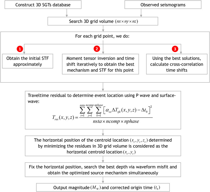
FIGURE 1. The brief inversion workflow for the source parameters.
Raw Data Processing
The continuous waveform data of the Changning earthquake can be downloaded from the China Seismic Experimental Site (CSES) website1 and we use 17 local broadband stations surrounding the epicenter to determine the source parameters in the study. These stations are distributed in Sichuan basin and four provinces of China with a good azimuth coverage and epicenter distances from 70 km to 370 km (Figure 2). After removing the mean, trend and instrumental responses, the displacement seismograms are cut to 400 s starting from the origin time, resampled with an interval of 0.04 s after lowpass filtering with corner frequency of 12.5 Hz, and then bandpass filtered to two period ranges (0.04–0.2 Hz and 0.03–0.1 Hz) respectively. The 2nd-order Butterworth filter with the same parameters is used for the seismograms and synthetic data.
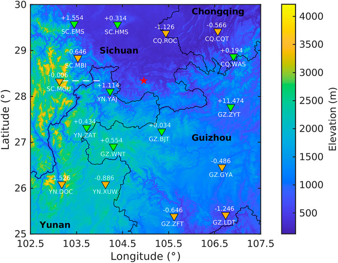
FIGURE 2. The topography in the study along with the centroid location of the Changning earthquake (red star) and 17 broadband stations (triangles) in the four provinces (black texts) of China. The white numbers above the triangles are the z-component time shifts of surface wave at stations (positive in green and negative in yellow) in Figure 10. The white texts below the triangles denote the names of seismic network and stations and the white dashed line marks the location of grid profile in Figure 5.
3D SGTs Construction
3D Model and Topography
Compared with averaged 1D layered models, a 3D velocity model shows more advantages in the estimation of the source parameters to obtain the more reliable solution, especially the light to moderate earthquakes (Johnson and Vincent, 2002; Hejrani et al., 2017; Nayak and Dreger, 2018; Wang and Zhan, 2019). In this study, we use the 3D P- and S-wave velocity model of the crust and uppermost mantle in the southwest China (SWChinaCVM-1.0, doi: 10.12093/02md.02.2019.01.v1) to compute the synthetics. The 3D model is obtained by the joint body and surface wave traveltime tomography, which involves 390,000 P-wave and 370,000 S-wave first-arrival traveltimes from more than 230 permanent stations and 8,100 dispersion curves of surface-wave phase velocity (5–50 s) extracted from the ambient noise data (Fang et al., 2016; Liu et al., 2020). The horizontal resolution of the model is about 50 km and the depth ranges from the surface to 70 km with an interval of 5 km. We extend the 3D model to 100 km in depth using the velocity at the depth of 70 km. Figures 3, 4 show the map view and two profiles of the P-wave velocity and S-wave velocity across the event location in the study area.
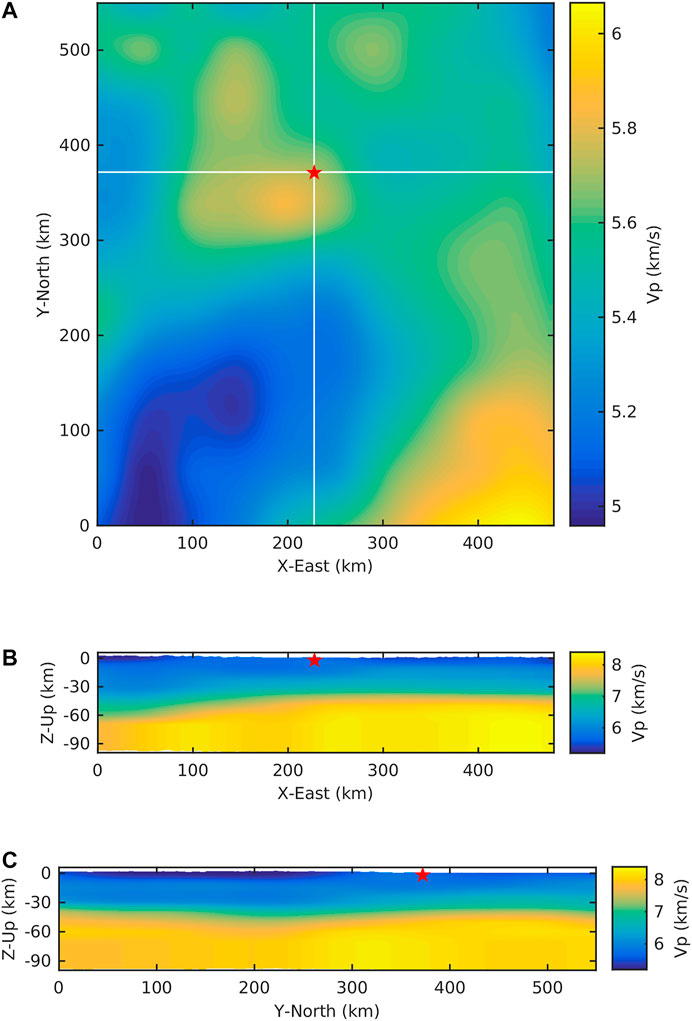
FIGURE 3. The map view and two profiles of the 3D P-wave velocity model across the event location (red star). The horizontal and vertical white lines in map view (A) show the location of XOZ profile (B) and YOZ profile (C) respectively.
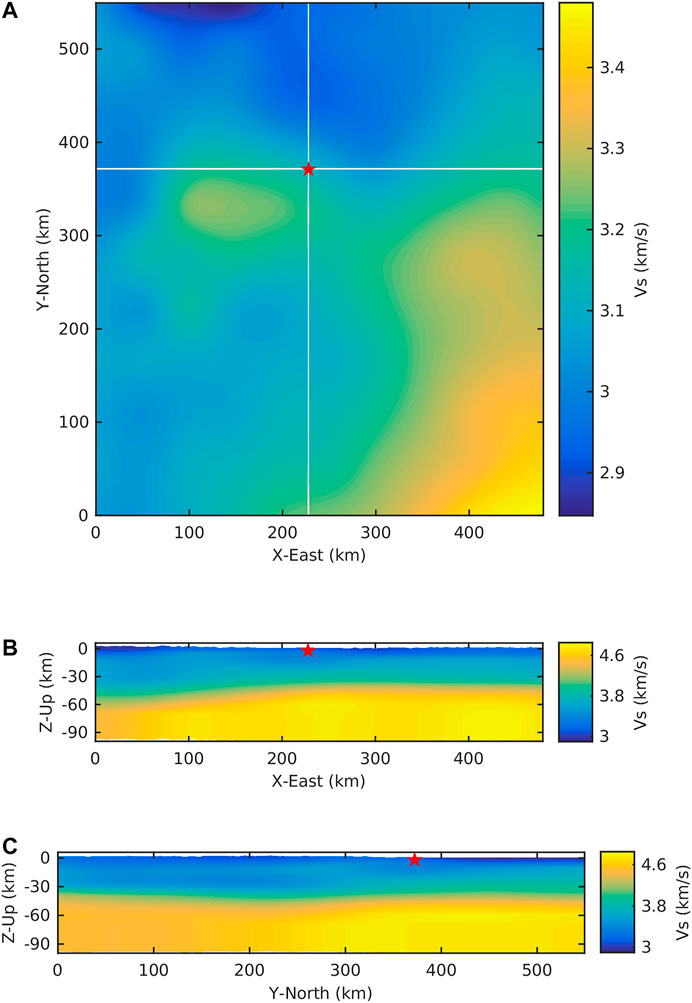
FIGURE 4. As in Figure 3, but for S-wave velocity.
The Changning earthquake occurs in the south of Sichuan basin and the east of the Tibetan plateau. The elevation in the study area rises from about 200 m in the south of Sichuan basin to over 4,000 m of Longmenshan Mountain within a very short distance (Figure 2). In order to accurately calculate the SGTs database, we should consider and handle the effect of the topography on the results. We utilize the topography data with a spatial resolution of approximately 90 m from CGIAR-CSI SRTM website2 and perform the down sampling of 500 m as the preparation of the next step.
Numerical Simulation by Curvilinear-Grid Finite-Difference
The traditional finite-difference methods commonly apply the strategy of grid refinement to fit the surface shape as much as possible, but it cannot avoid the artifacts due to the staircase approximation. We use the curvilinear-grid finite-difference approach with the Traction Image free surface boundary implementation (Zhang and Chen, 2006; Zhang et al., 2012) to construct the SGTs database in the 3D model with the rugged topography of this region. Figure 5 shows the partial curvilinear grids along one vertical profile (XOZ) as marked with dashed line in Figure 2.
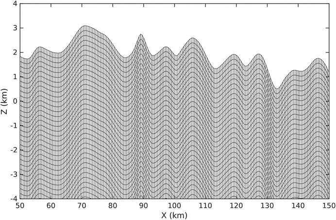
FIGURE 5. The curvilinear grids along one vertical profile (white dashed line in Figure 2) in the presence of the topography of the region.
Generally, the number of forward modeling is proportional to the total number of potential source points, which seems not feasible for the large 3D grid volume. Fortunately, we can adopt the reciprocity theorem and calculate the SGTs from each station to all source points instead of computing the Green’s functions source by source (Eisner and Clayton, 2001; Zhao et al., 2006). In this way, the number of the simulations is reduced to the three times of the total number of stations when the three-component data are needed, which dramatically saves the computational costs. Using the SGTs, the calculated displacements at the station
where
The geographical coordinates are projected to the Cartesian coordinates with the reference origin point (25.0°N, 102.5°E). The computational model size in the study area is 480 km × 550 km × 100 km with a horizontal grid spacing of 500 m. We employ the complex-frequency-shifted perfectly matched layer based on auxiliary differential equations (ADE CFS-PML) technique and configure 12 layers as the non-reflecting boundaries in the forwarding modeling (Zhang and Shen, 2010). For accurately simulating the surface wave in the presence of the rugged topography, we set the vertical grid spacing to 200 m. Thus, the number of grid points for three dimensions becomes 960 × 1,100 × 500. The simulated maximum frequency reaches 0.5 Hz and the sampling interval is set to 0.02 s derived from the minimum grid spacing and the maximum velocity. The recording time length is 400 s along with a total number of time steps of 20,000. The calculation of SGTs for 17 stations totally costs about 160 thousand CPU hours. We save the SGTs of a 3D grid volume (200 × 200 × 140) in the neighborhood of the epicenter from CENC with a mesh of 500 m × 500 m × 200 m and an interval of 0.04 s, resulting about 95 TB of total storage for the 17 broadband stations. We use the cubic-spline interpolation approach to retrieve the SGTs at the finer grids (200 m × 200 m × 10 m) near the event to improve the resolution of location and depth.
Source Mechanism Estimation in Each Trial Point
In this step, we optimize the source mechanism in each trial source point of 3D grid volume in terms of the initial solutions from Global CMT. With the representation of the synthetics using Eq. 1, the moment tensors can be linearly inversed by solving the normal equation:
and
where
The frequency bands in the inversion are relatively low, so we can use a simple function to approximate the complex real STF and ignore the high-frequency variations. We choose the bell function as the form of the STF (moment-rate function). The source duration
where
Specifically, the optimal moment tensors and STF in each trial source point are determined by the following procedures. We first use the source mechanism from Global CMT as the initial approximated solution to calculate the synthetics. Then we cross-correlate the observed and the synthetic waveforms to obtain the time shifts for each component of P- and surface waves. After aligning the SGTs with the corresponding time shifts, we can solve the Eq. 2 to determine the moment tensors. Subsequently, the calculated moment tensors are considered as the new initial source mechanism to the next inversion. The inversion procedures can be carried out repeatedly until both of moment tensors and STF become stable for each trial point.
Horizontal Position Locating
For each trial source point in 3D grid volume, we obtain the optimal source mechanism and STF at this point that can best fit the observed seismograms in Source Mechanism Estimation in Each Trial Point. Then, the time shifts of the P wave and surface wave are derived by cross-correlating the observation and the synthetics for all stations. The traveltime residual
where
The weighting factor of
Figure 6 shows the map of the traveltime misfit with a grid size of 1 km × 1 km at the event depth (3.14 km) of Changning earthquake which is determined later by minimizing the waveform misfit in Event Depth Determination. The coordinates of initial location are 235.1 km (X) and 371.8 km (Y). The searching X-coordinate ranges from 199.5 km to 298.5 km and the Y-coordinate ranges from 324.5 km to 423.5 km. A nest grid search strategy and a local finer searching with the grid size of 200 m is applied to accelerate the locating process and refine the centroid location. The map illustrates the reasonable characteristics of the misfit value increasing gradually with the grid far away the true location. In addition, the three contours near the event show that the error distribution does not exhibit apparently directional pattern.
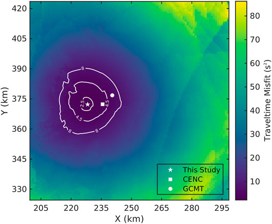
FIGURE 6. The traveltime misfit map along with three contours (white lines), the centroid location in this study (white star), epicenter location by CENC (white square) and centroid location by Global CMT (white dot) at the event depth (3.14 km).
Besides, we also plot the traveltime misfit maps with a coarse grid size of 6 km × 6 km at the various depths from 1.2 km to 27.7 km (Figure 7). From the top to the bottom, the patterns of the misfit distribution exhibit generally consistent except for some little anomalies probably caused by model complexities.
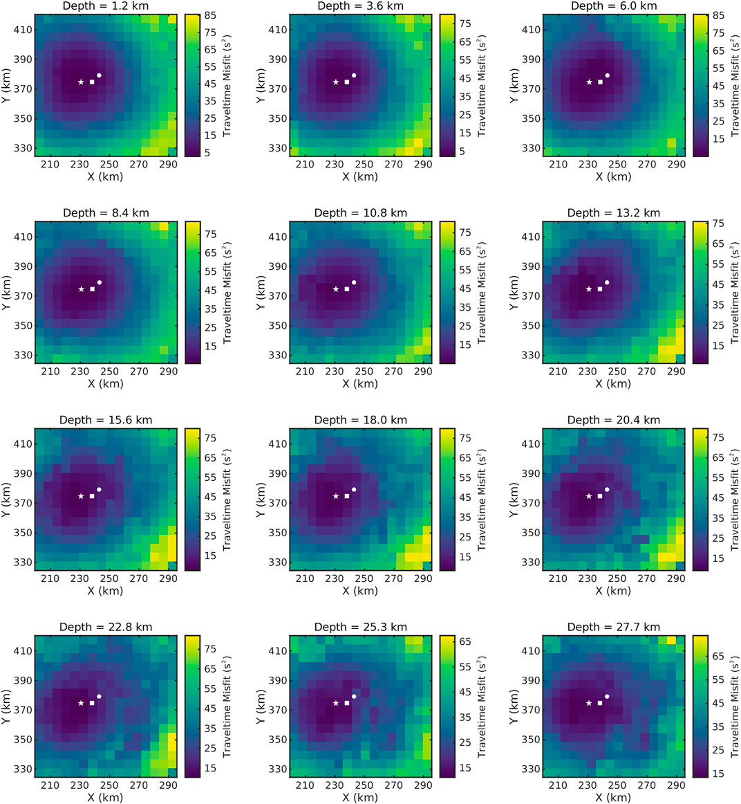
FIGURE 7. Traveltime misfit maps along with the centroid location in this study (white star), epicenter location by CENC (white square) and centroid location by Global CMT (white dot) at various depth from 1.2 km to 27.7 km.
Event Depth Determination
The traveltime information has a better constraint on the horizontal position of the event, but it is not suitable for the estimation of the event depth unless the epicenter distances are short enough relative to the depth. Nevertheless, the waveform misfits in terms of L2 norm between the observation and the synthetics are sensitive to the variation of hypothetical depth. As a consequence, we minimize the waveform misfits at different depths to find the optimal event depth while the horizontal location is fixed for each calculation. The corresponding source mechanism and STF in the optimal depth are accepted as the final solution. As the Figure 8 shows, the waveform misfit reaches a minimum when the trial depth is 3.14 km.
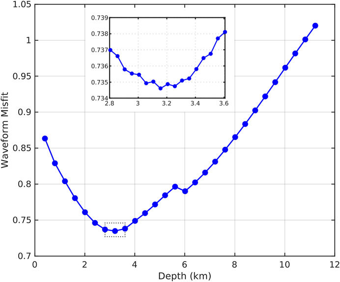
FIGURE 8. The curve of waveform misfits vs. trial event depths with the horizontal location fixed. The middle solid rectangle is a partial enlarged drawing for local smaller grid-searching size (50 m) from 2.8 km and 3.6 km depth.
The moment magnitude can be easily derived from the source mechanism by Eq. 6 and the formulas proposed by Hanks and Kanamori (1979). Based on the event location from Horizontal Position Locating and Event Depth Determination, the origin time is also updated with the correction item from Eq. 8.
Results
Table 1 summarizes the source parameters of the Changning earthquake in this study, Global CMT, Liu and Zahradník (2020), and CENC. The origin time (2019-06-17 14:55:45.0 GMT) in this study is about 2 s earlier than Global CMT and 2 s behind CENC. The magnitude results are almost the same among these reports excluding that of CENC in MS. The horizontal centroid position in our research (28.34°N, 104.82°E) is located on the west of the others and has a maximum distance deviation of about 15 km with respect to Global CMT, which is possibly caused by the effects of the local 3D model we used. With the optimization of waveform misfit along depth, we find the final event depth is 3.14 km which is the shallowest among all the results and very close to the operation geological layer of shale gas in Sichuan basin. The two nodal planes are strike 295°/dip 88°/rake 14° and strike 204°/dip 76°/rake 178°. The moment tensors are decomposed to DC, CLVD and ISO components using the method proposed by Knopoff and Randall (1970), with the percentages of 10, −83 and −7% respectively. The optimum duration of STF is 3.48 s. The comparison of beachballs between this study and the other two agencies is shown as Figure 9. The shaded areas among the three beachballs are similar and nodal planes of the DC part of the moment tensor are not the same which could be explained by the low DC percentage. Overall, our results are in agreement with the other two agencies.
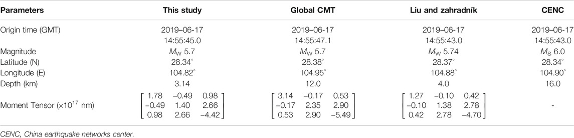
TABLE 1. The source parameters of Changning earthquake from different affiliations.
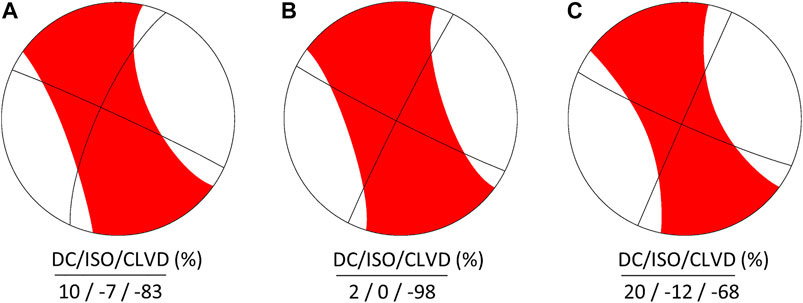
FIGURE 9. The beachballs along with the fault plane solutions and the percentages of DC, ISO and CLVD components at the bottom of each panel (A) This study (B) Global GMT (C)Liu and Zahradník (2020).
The reliability of our results in Table 1 can be evaluated by comparing the observed seismograms and the synthetic waveforms. Figure 10 shows the waveform fitting of six segments from three-component P waves (0.04–0.2 Hz) and surface waves (0.03–0.1 Hz) at all stations. The waveforms in each segment are aligned with the cross-correlation time shifts. In the determination of the event location, these time shifts with large deviations relative to the other two components for the same phase are abandoned directly, which is possibly caused by the insufficiency of the used 3D model. Specifically, they are E components of surface wave at BJT and HMS station, Z component of surface wave at ZYT station as marked with red rectangles in Figure 10. In addition, the corresponding time shifts in these segments with bad quality
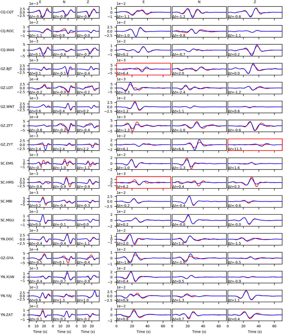
FIGURE 10. The waveform fitting of the three-component (ENZ) P wave (left three columns, 0.04–0.2 Hz) and the surface wave (right three columns, 0.03–0.1 Hz) at all stations utilized for inversion. The leftmost texts in each row mark the seismic network and station names. The red and blue solid lines indicate the observation and the synthetic data using the optimum source position and mechanism respectively along with the time shift below each waveform. The red rectangles mark the segments in which the time shifts are not used in the calculation of traveltime residuals.
Apart from the analysis of waveform fitting segment by segment, we also plot the whole observed seismograms and synthetics without the artificial time alignment at each station in Figure 11, 12. The seismograms at all stations are starting from the same origin time in Table 1 and then bandpass filtered with 0.03–0.06 Hz (Figure 11) and 0.03–0.1 Hz (Figure 12) as well as the synthetics. We can observe the waveforms at most of stations fit very well except for the ZYT and HMS station which could be caused by the possible error in absolute timing at ZYT station and in sensor orientation at HMS station.
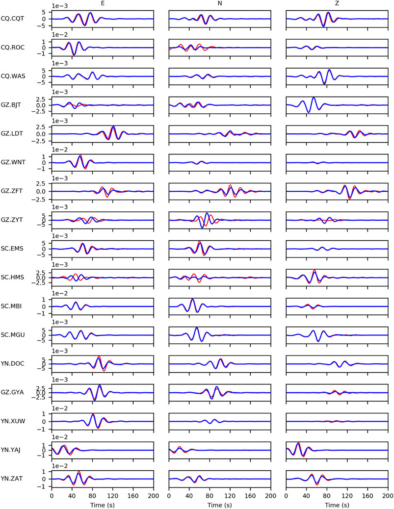
FIGURE 11. The waveform fittings (0.03–0.06 Hz) of the whole three-component data at all stations with the origin time of Table 1. The red and blue solid lines indicate the observation and the synthetic data using the optimum source position and mechanism, respectively. Here, the artificial time shifts are not applied. The leftmost texts in each row mark the seismic network and station names.
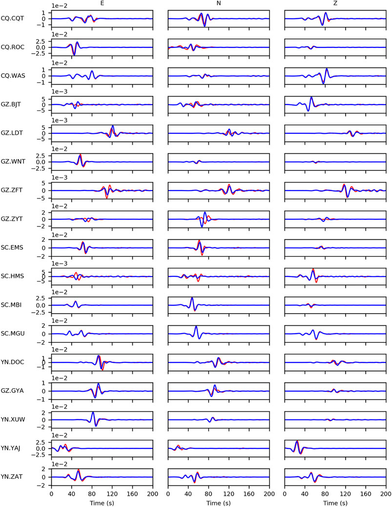
FIGURE 12. As in Figure 11, but for frequency range of 0.03–0.1 Hz.
While the horizontal centroid location is fixed, the uncertainties of the event depth and moment tensors for the Changning earthquake are estimated by the bootstrapping method (Efron and Tibshirani, 1991; Zhan et al., 2012) with 17 stations resampled independently for 1,000 times totally. The bootstrapping results show that the percentages of DC and ISO components do not have very small uncertainties with standard deviations (STD) of 10.5% and 8.1% respectively, which are possibly caused by their low percentages in moment tensor (Supplementary Figure S1A,B in Supplementary Material). The CLVD exhibits a little bit larger STD of 15.0% but with about 65% of the statistics more than 70%, indicating the confident existence of the large CLVD component (Supplementary Figure S1C). The Kagan angle (K-angle) is defined as the minimum rotation angle between two focal mechanisms, which can be employed to transfer one focal mechanism to the other (Kagan, 1991). The focal mechanisms are regarded as similar with K-angle among them less than 30° and significantly different for larger than 40° (Zahradník and Custódio, 2012; Dias et al., 2016). The average K-angle with respect to the presented fault-plane solution in Results is 26.3°, indicating good consistency between our results and those in the bootstrapping test (Supplementary Figure S1D). The small STD (0.4 km) shown as Supplementary Figure S1E illustrates the event depth is well constrained in this study. Similarly, the centroid location is relocated many times with the same configuration of bootstrapping but using moment tensor and depth in Table 1. The local refinement of grid (200 m × 200 m) in the locating step is not applied but with overall grid size of 1 km × 1 km for efficiency. The estimated STDs of X- and Y-coordinate are 2.7 km and 1.6 km respectively (Supplementary Figure S1F,G). The azimuth gaps of the current seismic network possibly become large in some directions if several stations are removed in the resampling of bootstrap, which could affect the uncertainty estimate. From our perspective, more stations used with better coverage will reduce the uncertainty of the Changning earthquake and other local events in the further study.
Discussions
The attenuation factors are not incorporated in the construction of SGTs database by curvilinear-grid finite-difference simulation in this study. We estimate the average quality factors of P- and surface waves (QP ≈ 500 and QS ≈ 500) at the depth of 5 km in this region from Dai et al. (2020). The distances from the Changning earthquake to 17 broadband stations range from 70 km to 370 km. In terms of the used frequency bands, the amplitudes with attenuation for P- and surface waves at the farthest station decrease to about 96% of the simulated amplitudes without attenuation by approximately multiplying an exponential term. The effects of attenuation on the determination of source parameters would be very small.
Besides, in order to evaluate the effects of topography and 3D complexities on the centroid location and moment tensors, we perform another two tests for 3D non-topography model (Supplementary Figures S3, S4) and 1D model in Supplementary Material. The 1D model is extracted from the 3D model at the horizontal centroid location from the surface to the bottom (Supplementary Figure S8). The comparisons of the source parameters of Changning earthquake are summarized in Supplementary Table S1. Compared with results in 3D model with topography, the event latitude and depth for 3D non-topography model have a difference of 1.4 km and 60 m respectively. The results for 1D model show larger difference of 3.0 km in latitude, 0.8 km in longitude and 160 m in depth. Supplementary Figure S2 shows the beachballs along with nodal plane and the percentages of the decomposed DC, ISO and CLVD components for the three models. The pattern of nodal planes for 1D model exhibits large variances with 3D model and 3D non-topography model. Although K-angle of the mechanism found in the 1D solution with respect to the 3D solution with topography is about 35°, it is still within 95% confidence region of the K-angle bootstrap variation in Supplementary Figure S1D. Using the source parameters in Supplementary Table S1, we plot the waveform fit for 3D non-topography model (Supplementary Figure S5–S7) and 1D model (Supplementary Figure S9–S11), respectively. Because the frequency bands we used are relatively low, the consideration of topography has no significant improvement on the waveform comparison. If we move to the higher frequency in the inversion, the distortion of waveform due to the topography will play a more important role in the results analysis. Although the waveform fit is very similar between Figures 10–12 and Supplementary Figure S5–S7, the moment tensor components and its decomposition change indeed when the topography is ignored. Supplementary Figure S9–S11 show an overall good fit except for the shifts on some stations, indicating the 1D model extracted in this way is a feasible and reliable approximation of 3D model.
Conclusion
The 2019 MW 5.7 Changning earthquake caused huge economic losses and casualties, which is the largest earthquake recorded in southern Sichuan basin. There are many studies reporting this event, but the location, depth and source mechanism of them are different each other. In this study, we use 3D SGTs to obtain centroid location, moment tensors and other source parameters of the Changning earthquake. The 3D SGTs are calculated by curvilinear-grid finite-difference method with the 3D model of southwest China considering the rugged topography of this region. The event location is derived by minimizing the traveltime residuals of P wave and surface wave in the candidate 3D grid volume and the depth is determined by the minimum waveform misfit along trial depths between the observations and the synthetics when the horizontal location is fixed. Based on the waveform inversion, we refine the event location to (28.34°N, 104.82°E) and the optimized depth is 3.14 km. The strike, dip and rake angles for the nodal planes are 295°/88°/14° and 204°/76°/178°. The moment tensors can be decomposed to DC, CLVD and ISO components with the percentages of 10, −83, and −7% respectively. The waveform fit for the corrected origin time (2019-06-17 14:55:45.0 GMT) is good, and it indicates the reliability of the results.
Data Availability Statement
Publicly available datasets were analyzed in this study. This data can be found here: China Seismic Experimental Site (CSES) website (http://124.17.4.85/wp-content/uploads/2019/06/wave_6.1.rar).
Author Contributions
YH accomplishes the processing of raw data, the programming of the inversion codes and the writing of the manuscript. WZ proposes the main ideas of the study and participates in the writing of the manuscript. The curvilinear-grid finite-difference codes were written by WZ in 2006 and continuously developed by our research group. JZ helps discuss the results and provides many useful instructions and suggestions. All authors contribute the revisions and the editing before submission.
Funding
The project is supported by the China Earthquake Science Experiment Project of the China Earthquake Administration (Grant No. 2018CSES0101), the National Natural Science Foundation of China (Grant No. U1901602) and Shenzhen Science and Technology Program (Grant No. KQTD20170810111725321).
Conflict of Interest
The authors declare that the research was conducted in the absence of any commercial or financial relationships that could be construed as a potential conflict of interest.
Acknowledgments
We thank the three reviewers for their insightful comments which greatly improve the manuscript. The continuous waveform data of the Changning earthquake are downloaded from the repository of the China Seismic Experiment Site (Wave 6.1. CSES Scientific Products, doi: 10.12093/01db.01.2019.03.v1). The instrumental responses are obtained from the Seismic Data Management Center of China (http://www.seisdmc.ac.cn/). The topography data are download from the CDIAR-CSI SRTM website (https://srtm.csi.cgiar.org/srtmdata/). Figures in this study are partly created using the GMT (http://gmt.soest.hawaii.edu/home).
Supplementary Material
The Supplementary Material for this article can be found online at: https://www.frontiersin.org/articles/10.3389/feart.2021.642721/full#supplementary-material.
Footnotes
1http://124.17.4.85/wp-content/uploads/2019/06/wave_6.1.rar
2https://srtm.csi.cgiar.org/srtmdata/
References
Clarke, H., Eisner, L., Styles, P., and Turner, P. (2014). Felt seismicity associated with shale gas hydraulic fracturing: the first documented example in Europe. Geophys. Res. Lett. 41 (23), 8308–8314. doi:10.1002/2014GL062047
Dai, A., Tang, C.-C., Liu, L., and Xu, R. (2020). Seismic attenuation tomography in southwestern China: insight into the evolution of crustal flow in the Tibetan Plateau. Tectonophysics 792, 228589. doi:10.1016/j.tecto.2020.228589
Dias, F., Zahradník, J., and Assumpção, M. (2016). Path-specific, dispersion-based velocity models and moment tensors of moderate events recorded at few distant stations: examples from Brazil and Greece. J. South Am. Earth Sci. 71, 344–358. doi:10.1016/j.jsames.2016.07.004
Efron, B., and Tibshirani, R. (1991). Statistical data analysis in the computer age. Science 253 (5018), 390–395. doi:10.1126/science.253.5018.390
Eisner, L., and Clayton, R. W. (2001). A reciprocity method for multiple-source simulations. Bull. Seismological Soc. America 91 (3), 553–560. doi:10.1785/0120000222
Ekström, G., and Engdahl, E. R. (1989). Earthquake source parameters and stress distribution in the Adak Island region of the central Aleutian Islands, Alaska. J. Geophys. Res. 94 (B11), 15499–15519. doi:10.1029/JB094iB11p15499
Ekström, G., Nettles, M., and Dziewoński, A. M. (2012). The global CMT project 2004-2010: centroid-moment tensors for 13,017 earthquakes. Phys. Earth Planet. Interiors 200-201, 1–9. doi:10.1016/j.pepi.2012.04.002
Ellsworth, W. L. (2013). Injection-induced earthquakes. Science 341 (6142), 1225942. doi:10.1126/science.1225942
Fang, H., Zhang, H., Yao, H., Allam, A., Zigone, D., Ben-Zion, Y., et al. (2016). A new algorithm for three-dimensional joint inversion of body wave and surface wave data and its application to the Southern California plate boundary region. J. Geophys. Res. Solid Earth 121 (5), 3557–3569. doi:10.1002/2015JB012702
Gan, W., Zhang, P., Shen, Z.-K., Niu, Z., Wang, M., Wan, Y., et al. (2007). Present-day crustal motion within the Tibetan Plateau inferred from GPS measurements. J. Geophys. Res. 112 (B8), B08416. doi:10.1029/2005JB004120
Goebel, T. H. W., and Brodsky, E. E. (2018). The spatial footprint of injection wells in a global compilation of induced earthquake sequences. Science 361 (6405), 899–904. doi:10.1126/science.aat5449
Grigoli, F., Cesca, S., Rinaldi, A. P., Manconi, A., López-Comino, J. A., Clinton, J. F., et al. (2018). The November 2017 MW 5.5 Pohang earthquake: a possible case of induced seismicity in South Korea. Science 360 (6392), 1003–1006. doi:10.1126/scienceaat201010.1126/science.aat2010
Hanks, T. C., and Kanamori, H. (1979). A moment magnitude scale. J. Geophys. Res. 84 (B5), 2348–2340. doi:10.1029/JB084iB05p02348
Hejrani, B., Tkalčić, H., and Fichtner, A. (2017). Centroid moment tensor catalogue using a 3-D continental scale Earth model: application to earthquakes in Papua New Guinea and the Solomon Islands. J. Geophys. Res. Solid Earth 122 (7), 5517–5543. doi:10.1002/2017JB014230
Jiang, D., Zhang, S., and Ding, R. (2020). Surface deformation and tectonic background of the 2019 Ms 6.0 Changning earthquake, Sichuan basin, SW China. J. Asian Earth Sci. 200, 104493. doi:10.1016/j.jseaes.2020.104493
Johnson, M., and Vincent, C. (2002). Development and testing of a 3D velocity model for improved event location: a case study for the India-Pakistan region. Bull. Seismological Soc. America 92 (8), 2893–2910. doi:10.1785/0120010111
Kagan, Y. Y. (1991). 3-D rotation of double-couple earthquake sources. Geophys. J. Int. 106 (3), 709–716. doi:10.1111/j.1365-246X.1991.tb06343.x
Knopoff, L., and Randall, M. J. (1970). The compensated linear-vector dipole: a possible mechanism for deep earthquakes. J. Geophys. Res. 75 (26), 4957–4963. doi:10.1029/JB075i026p04957
Lei, X., Huang, D., Su, J., Jiang, G., Wang, X., Wang, H., et al. (2017). Fault reactivation and earthquakes with magnitudes of up to Mw4.7 induced by shale-gas hydraulic fracturing in Sichuan Basin, China. Sci. Rep. 7, 7971. doi:10.1038/s41598-017-08557-y
Lei, X., Su, J., and Wang, Z. (2020). Growing seismicity in the Sichuan Basin and its association with industrial activities. Sci. China Earth Sci. 63, 1633–1660. doi:10.1007/s11430-020-9646-x
Lei, X., Wang, Z., Wang, Z., and Su, J. (2019). Possible link between long-term and short-term water injections and earthquakes in salt mine and shale gas site in Changning, south Sichuan Basin, China. Earth Planet. Phys. 3 (6), 510–525. doi:10.26464/epp2019052
Li, W., Ni, S., Zang, C., and Chu, R. (2020). Rupture directivity of the 2019 Mw 5.8 changning, sichuan, China, earthquake and implication for induced seismicity. Bull. Seismological Soc. America 110 (5), 2138–2153. doi:10.1785/0120200013
Liu, J., and Zahradník, J. (2020). The 2019 M W 5.7 changning earthquake, Sichuan basin, China: a shallow doublet with different faulting styles. Geophys. Res. Lett. 47 (4), e2019GL085408. doi:10.1029/2019GL085408
Liu, Y., Yao, H., Zhang, H., and Fang, H. (2020). The Community Velocity Model V1.0 of southwest China, constructed from joint body- and surface-wave traveltime tomography. Seismological Res. Lett. in press.
Long, F., Zhang, Z., Zhang, Z., Qi, Y., Liang, M., Ruan, X., et al. (2020). Three dimensional velocity structure and accurate earthquake location in Changning-Gongxian area of southeast Sichuan. Earth Planet. Phys. 4 (2), 1–15. doi:10.26464/epp2020022
Ma, X. (2017). A golden era for natural gas development in the Sichuan Basin. Nat. Gas Industry B 4 (3), 163–173. doi:10.1016/j.ngib.2017.08.001
Meng, L., McGarr, A., Zhou, L., and Zang, Y. (2019). An investigation of seismicity induced by hydraulic fracturing in the Sichuan basin of China based on data from a temporary seismic network. Bull. Seismological Soc. America 109 (1), 348–357. doi:10.1785/0120180310
Myers, S. C., Simmons, N. A., Johannesson, G., and Matzel, E. (2015). Improved regional and TeleseismicP‐wave travel‐time prediction and event location using a global 3D velocity model. Bull. Seismological Soc. America 105 (3), 1642–1660. doi:10.1785/0120140272
Nayak, A., and Dreger, D. S. (2018). Source inversion of seismic events associated with the sinkhole at napoleonville salt dome, Louisiana using a 3D velocity model. Geophys. J. Int. 214 (3), 1808–1829. doi:10.1093/gji/ggy202
Tan, Y., Hu, J., Zhang, H., Chen, Y., Qian, J., Wang, Q., et al. (2020). Hydraulic fracturing induced seismicity in the southern Sichuan Basin due to fluid diffusion inferred from seismic and injection data analysis. Geophys. Res. Lett. 47 (4), e2019GL084885. doi:10.1029/2019GL084885
Wang, M., and Shen, Z. K. (2020). Present‐Day crustal deformation of continental China derived from GPS and its tectonic implications. J. Geophys. Res. Solid Earth 125 (2), e2019JB018774. doi:10.1029/2019JB018774
Wang, S., Jiang, G., Weingarten, M., and Niu, Y. (2020). InSAR evidence indicates a link between fluid injection for salt mining and the 2019 Changning (China) earthquake sequence. Geophys. Res. Lett. 47 (16), e2020GL087603. doi:10.1029/2020GL087603
Wang, X., and Zhan, Z. (2019). Moving from 1-D to 3-D velocity model: automated waveform-based earthquake moment tensor inversion in the Los Angeles region. Geophys. J. Int. 220 (1), 218–234. doi:10.1111/j.1365-246X.2012.05472.x10.1093/gji/ggz435
Yi, G., Long, F., Liang, M., Zhao, M., Wang, S., Gong, Y., et al. (2019). Focal mechanism solutions and seismogenic structure of the 17 June 2019 MS 6.0 Sichuan Changning earthquake sequence. Chin. J. Geophys. (in Chinese) 62 (9), 3432–3447. doi:10.6038/cjg2019N0297
Zahradník, J., and Custódio, S. (2012). Moment tensor resolvability: application to Southwest Iberia. Bull. Seismological Soc. America 102 (3), 1235–1254. doi:10.1785/0120110216
Zhan, Z., Helmberger, D., Simons, M., Kanamori, H., Wu, W., Cubas, N., et al. (2012). Anomalously steep dips of earthquakes in the 2011 Tohoku-Oki source region and possible explanations. Earth Planet. Sci. Lett. 353-354, 121–133. doi:10.1016/j.epsl.2012.07.038
Zhang, B., Lei, J., and Zhang, G. (2020). Seismic evidence for influences of deep fluids on the 2019 Changning Ms 6.0 earthquake, Sichuan basin, SW China. J. Asian Earth Sci. 200, 104492. doi:10.1016/j.jseaes.2020.104492
Zhang, W., and Chen, X. (2006). Traction image method for irregular free surface boundaries in finite difference seismic wave simulation. Geophys. J. Int. 167 (1), 337–353. doi:10.1111/j.1365-246X.2006.03113.x
Zhang, W., and Shen, Y. (2010). Unsplit complex frequency-shifted PML implementation using auxiliary differential equations for seismic wave modeling. Geophysics 75 (4), T141–T154. doi:10.1190/1.34634310.1190/1.3463431
Zhang, W., Zhang, Z., and Chen, X. (2012). Three-dimensional elastic wave numerical modelling in the presence of surface topography by a collocated-grid finite-difference method on curvilinear grids. Geophys. J. Int. 190 (1), 358–378. doi:10.1111/j.1365-246X.2012.05472.x
Zhao, L., Chen, P., and Jordan, T. H. (2006). Strain green's tensors, reciprocity, and their applications to seismic source and structure studies. Bull. Seismological Soc. America 96 (5), 1753–1763. doi:10.1785/0120050253
Zhao, L., and Helmberger, D. V. (1994). Source estimation from broadband regional seismograms. Bull. Seismological Soc. America 84 (1), 91–104.
Zhao, Z., and Zhang, R. (1987). Primary study of crustal and upper mantle velocity structure of Sichuan Province. Acta Seismologica Sinica 9 (2), 154–166.
Zhou, L., Zhang, W., Shen, Y., Chen, X., and Zhang, J. (2016). Location and moment tensor inversion of small earthquakes using 3D Green's functions in models with rugged topography: application to the Longmenshan fault zone. Earthq Sci. 29 (3), 139–151. doi:10.1007/s11589-016-0156-1
Zhu, L., and Helmberger, D. V. (1996). Advancement in source estimation techniques using broadband regional seismograms. Bull. Seismological Soc. America 86 (5), 1634–1641.
Zhu, L., and Zhou, X. (2016). Seismic moment tensor inversion using 3D velocity model and its application to the 2013 Lushan earthquake sequence. Phys. Chem. Earth, Parts A/B/C 95, 10–18. doi:10.1016/j.pce.2016.01.002
Keywords: changning earthquake, source mechanism, seismic location, 3D strain Green's tensors, topography
Citation: Huo Y, Zhang W and Zhang J (2021) Centroid Moment Tensor of the 2019 MW 5.7 Changning Earthquake Refined Using 3D Green’s Functions Considering Surface Topography. Front. Earth Sci. 9:642721. doi: 10.3389/feart.2021.642721
Received: 16 December 2020; Accepted: 04 February 2021;
Published: 22 March 2021.
Edited by:
Nicola Alessandro Pino, Vesuvius Observatory, National Institute of Geophysics and Volcanology (INGV), ItalyReviewed by:
Wenbo Wu, California Institute of Technology, United StatesXin Wang, California Institute of Technology, United States
Jiri Zahradnik, Charles University, Czechia
Copyright © 2021 Huo, Zhang and Zhang. This is an open-access article distributed under the terms of the Creative Commons Attribution License (CC BY). The use, distribution or reproduction in other forums is permitted, provided the original author(s) and the copyright owner(s) are credited and that the original publication in this journal is cited, in accordance with accepted academic practice. No use, distribution or reproduction is permitted which does not comply with these terms.
*Correspondence: Wei Zhang, emhhbmd3ZWlAc3VzdGVjaC5lZHUuY24=