 Chenghao Cao
 Li-Yun Fu
 Bo-Ye Fu
 Qiang Guo
- 1College of Transportation Science & Engineering, Nanjing Tech University, Nanjing, China
- 2Key Laboratory of Deep Oil and Gas, China University of Petroleum (East China), Shandong, China
- 3Institute of Geology and Geophysics, Chinese Academy of Sciences (CAS), Beijing, China
- 4College of Information Engineering, China Jiliang University, Hangzhou, China
Elastic interactions between fractures will greatly affect the effective elasticity, which, in turn, will reshape the effective fracture parameters. The disturbance will be more complex in the fault zone due to the complicated fracture distributions. This problem is addressed by the comparison of two types of solutions: one containing the stress interaction while the other one excluding the stress interaction. The gap between the two solutions allows the quantitative estimation of stress interactions on elasticity. Furthermore, based on the orthorhombic assumption for fracture clustering in the damage zone, the effect of stress interaction on the equivalent fracture parameter is estimated. We first characterize the fracture parameters in the fault damage zone considering more realistic distributions of fractures. Then, a series of numerical simulations are conducted to study the effective parameters of the fractured model. Finally, assuming the orthorhombic system of the fracture clustering, we invert the crack density and validate the accuracy of the inversion through the incidence angle seismic velocities. Our numerical results suggest that the size of fractures will determine the dominant type of stress interactions, and thus significantly reshape the effective properties of the models regardless of the spatial distribution of the fracture. Furthermore, the stress interactions tend to underestimate the fracture density for models containing long fractures but generate a relatively satisfactory inverted fracture density for short fractures.
Introduction
In general, local stress distribution generated by a single crack hardly influences their neighbors for a sparse concentration for cracks, which, however, would be significant as the crack density exceeds the dilute limit (Zhao et al., 2015; Cao et al., 2020a). That is, for a small fracture density, the resultant effective compliance tensor depends linearly on the crack density but non-linearly for a high concentration for cracks, implying a non-negligible effect of stress interactions.
Actually, there are two types of stress interactions, namely shielding and amplification, with opposite signs (Cao et al., 2019). Stress shielding considerably stiffens rocks while stress amplification appreciably reduces the effective elasticity (Zhao et al., 2015). Furthermore, the shielding and amplification effect dominate for stacked cracks and co-planar cracks, respectively (Grechka and Kachanov, 2006b). The effect of stress interactions has been described by both numerical simulations and analytical expressions of the effective elasticity for the fractured media in a series of publications (Kachanov, 1993; Hopkins, 2000; Lapin et al., 2018; Cao et al., 2020a).
Many effective analytical medium theories have been developed for the fractured media, including the self-consistent theory (SC), differential effective medium (DEM) theory, and T-matrix solution (Jakobsen, 2012), and a comprehensive review of these theories can be found in Mavko et al. (2009). These methods could be used to characterize the mechanical properties of an effective sample considering the stress interactions. Besides the analytical solutions, a series of numerical solutions have also been developed for characterizing the fractured media (Masson and Pride, 2007). Using the finite-element (FE) solution, Wenzlau et al. (2010) obtain five independent elastic moduli in a heterogeneous layered medium. Similarly, Quintal et al. (2011) propose a computationally efficient method to solve Biot's quasi-static equations of consolidation. Furthermore, based on the solution, Quintal et al. (2012) also obtain S-wave attenuation for a medium containing periodically distributed circular inclusions. Due to the tectonic movement, the underground medium often behaves like a triclinic medium with the highest degree of anisotropy, which, however, is hard to describe using the aforementioned numerical methods. Therefore, a novelty numerical method, developed by Rubino et al. (2016), is used to solve the problem by generating complex-valued, frequency-dependent equivalent stiffness tensors, the advantage of which lies in the quantification of six elastic tensors for the two-dimensional (2D) case. However, neither the analytical nor the numerical solutions could explicitly identify the dominant type of stress interactions. Cao et al. (2020a) proposed a workflow to address the problem through the gaps between the analytical results without stress interactions and the numerical one with stress interactions, making the quantification of stress interaction possible.
The non-interaction approximation (NIA) or the linear slip (LS) theory treats the compliance tensors of the fractured rock as a sum of the compliance tensors of the host matrix plus individual fractures, which works well for a low concentration for cracks, and thus provides a benchmark for a quantitative estimation of stress interactions. However, when applied to fractured solids, NIA has a larger-than-expected range of applicability in the cases of dilute limit as well as the high fracture densities (Grechka and Kachanov, 2006b). The reason lies in that, the opposite effects of shielding and amplification largely cancel one another in the medium with the fractures distributed randomly (Lapin et al., 2018), thus making the result similar to that of the NIA solution.
Strictly speaking, only the equivalence between the normal fracture compliance and the shear fracture compliance could ensure the orthorhombic symmetry of the fractured medium (Schoenberg and Sayers, 1995). However, Kachanov (1993) believes that, in the NIA approximation, effective elasticity for the cracked model could also be orthorhombic. Based on this, Grechka (2007) extends the case to the transversely isotropic with a host with a vertical symmetry axis (VTI), which also satisfies the aforementioned orthorhombic assumption. Therefore, it is possible to retrieve some key parameters related to the fractured information based on seismic recordings such as fracture density (Barbosa et al., 2018).
In the damage zone, fractures often exhibit spatial variation in the petro-physical properties, such as characteristics of the fracture length distribution (Lei and Gao, 2018) and the spatial distribution for the fractures inside (Harris et al., 2003). In recent years, there have been some attempts at describing the fracture length distribution based on the power law. Hunziker et al. (2018) adopted the power law to describe the fracture length distribution for the systematic exploration of the attenuation sensitivity to the properties characterizing the fracture network. Lei and Gao (2018) also characterize the stress variability in geological media based on the assumed synthetic fracture networks following power law length scaling. On the other hand, the fracture also exhibits in some forms of spatial distribution (Odling et al., 2005). The aspect ratio (Ξ), proposed by Jakobsen et al. (2003), is used to characterize the fracture spatial distribution, which, however, is more complex in nature.
For example, the fracture clustering in the damage zone, often distributed in a complex pattern and, hence, characterizing realistic spatial distributions of fractures quantitatively, is necessary for an accurate interpretation of seismic measurements. Savage and Brodsky (2011) investigate the development of fracture spatial distributions as a function of displacement to determine whether damage around small and large faults is governed by the same process. Harris et al. (2003) also capture the characteristics of the damage zone using distance from the fault surface. Although the fracture clustering in the damage zone is a rather common scenario in nature, description of the effects of stress interaction on the elasticity and effective fracture parameters of the damage zone remains largely unexplored, partly due to the limitations of the analytical models as well as the high computational cost because of the complex fracture distribution.
In this study, the authors address this problem by the following procedures. First, we develop a numerical model for the fracture clustering in the 2D fault damage zone. This model includes the statistical parameters of the fault damage zones observed in outcrop, followed by the investigation of effective elasticity as well as anisotropic parameters of the models. Finally, assuming the damage zone possesses the orthorhombic symmetry in the NIA, the fracture parameters for two sets of orthogonal fractures are inverted, based on which we could obtain the incidence angle dependency of the seismic wave.
Generation of Fracture Clustering in the Fault Damage Zone
For modeling the fracture clustering in the fault damage zones, the characteristics of the fracture system must be quantified in advance, including fracture length distribution, spatial distribution, and orientation distributions. Therefore, in the following section, detailed information about these characteristics, and how they are systematically incorporated into numerical models, is introduced.
Rules for the Fracture Length
The power law for fracture length distribution (Bonnet et al., 2001) is often used to characterize the natural fracture system. The stochastic distribution m for the fracture length l (Hunziker et al., 2018) is expressed as:
where L is the scale of the modeling domain while Imin and Imax are the minimum and maximum fracture lengths, respectively. Furthermore, the maximum fracture length (Imax) is only one-third of the square length (L/3 = 0.33 m), because having fractures greater than half the sample size would mechanically weaken the sample. In this study, the size L of the sample was fixed at 1.0 m. Throughout the study, the aperture of the fracture is set to be 3 mm. The exponent a is the power law length exponent, which affects the relative probability of long and short fractures. A smaller a prefers the long fractures at the expense of the short fractures. Here, we would like to set two values for the length exponent, a = 1.5 and 3, which covers two scenarios, one dominated by long fractures and the other by short fractures, respectively.
The parameter dc is the fracture density term, defined as the number of fracture centers per unit area. However, throughout the study, the fracture density, e, (Equation 1) is used as defined by Guo et al. (2018), which is quite different from that defined by de Dreuzy et al. (2001). As for dc, we set it as a function of the fracture number as follows:
where n is the fracture number inside the 2D sample, with four different values (50, 100, 150, and 200) in our study. The constant 0.03 is an optimized parameter. For keeping the units unchanged, the factor L2 is imposed into equation 1 as the denominator.
Rules for Fracture Spatial Distribution
In addition to the aforementioned length distribution, particular focus is also given to characteristics of fracture spatial distribution, one of the most challenging tasks that remain to be unexplored.
For fracture clustering, the fracture density often decays away from the main fault. Moreover, for any fracture, except the fracture with the smallest length, there is a chance that a smaller fracture will be clustered about it. That is, each fracture is placed depending on the location of the long fracture.
To construct such a kind of fractured model, an ellipsoidal volume with the aspect ratio Ξ is generated. This ellipsoid is supposed to include all centers of the clustering fractures (Figure 1A). Then, the volume is divided into a series of concentric ellipsoidal shells (Figure 1B), which cuts the vertical principal axis into equal parts. The fractures are sorted by size scale and further divided equally into concentric shells. The centers of the largest fracture are located inside the smallest ellipsoidal shell. The successive clusters of fractures with decreasing scales are then located in successive shells, which are of increasing volume (Harris et al., 2003).
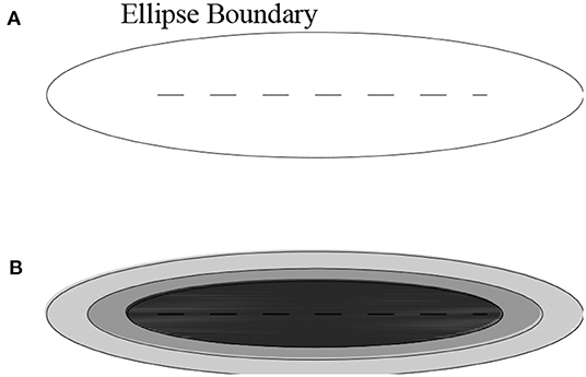
Figure 1. (A) The ellipsoid area, defined by the aspect ratio (Ξ), encompasses all fractures surrounding the major faults. (B) Concentric ellipsoidal shells around the major fault in (A). Each shell contains equal fractures, and thus, the resultant fracture density decreases gradually toward the outside. The darker area means a greater fracture density.
Based on the extended ellipse around the major fault, a random proportion of the area (black area in Figure 2) swept by a radius of this ellipsoidal volume is used to define an azimuthal angle θ and the radius OB (Figure 2). Compared with the adoption of the random angle, the use of the swept area (black zone in Figure 1) would produce a bias toward the major axis of the ellipse, which is more representative of the natural fault zone.
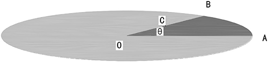
Figure 2. Location of the fracture center, C. The azimuthal angle θ as well as the radius OB could be defined according to the random black area swept out by a radius of this ellipse. Point C is chosen along OB using a normalized function (Equations 3, 4).
For the location of the fracture center C, the authors would like to introduce the normalized function, t(r), as the function of normalized distance, r, along with the radius OB, with r = 1 being the shell boundary and r = 0 being the shell center. The normalized function has the form given in equation 3:
where the value p = 0.15, which is used throughout this study, resembles a pyramid-like displacement profile, making the fractures distributed more evenly over the major fault.
For a better description of the generation of the numerical model, a workflow chart to describe the generation procedure is presented in Figure 3.
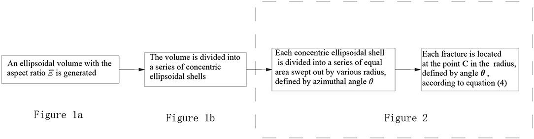
Figure 3. A work flow chart to describe the generation procedure for the fracture set in the damage zone.
Rules for Fracture Orientation
According to Harris et al. (2003), fractures inside both the Moab and Ninety Fathom fault damage zones are generally oriented sub-parallel to the major fault. Therefore, in the following models presented here, the strike of the fractures is set according to the Gaussian distribution law, each with a standard deviation of 10°.
A smaller Ξ results in a locally dense fracture clustering, thus leading to more fracture intersections, which, however, would bias the realistic fracture densities. Therefore, in this study, none of the fractures inside the models have intersections with each other.
Numerical Methodology
Methodology of the Numerical Simulation
Due to tectonic movement, the rock mass often shows a certain degree of deformation, resulting in the triclinic crystal models with the highest degree of anisotropy, which could characterize a homogeneous distribution of cracks.
In order to study the elastic properties of this complex medium, three numerical simulations with various boundary conditions are conducted here (Rubino et al., 2016) to obtain the elasticity matrix of the model. Detailed information about the process is given in Table 1 and as follows: (1) a fixed displacement is imposed on the upper boundary while keeping the vertical displacement to the other boundaries zero (Figure 4A); (2) the displacement is applied on the lateral side while keeping the displacement vertical to the other boundaries zero (Figure 4B); (3) a simple shear test is conducted (Figure 4C). The displacements Δu are all static rather than oscillatory.
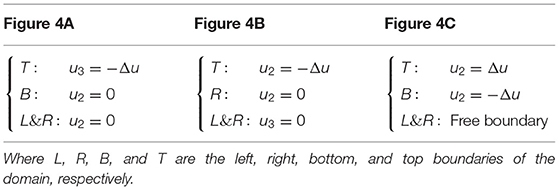
Table 1. The boundary conditions for the three models (Figure 4).
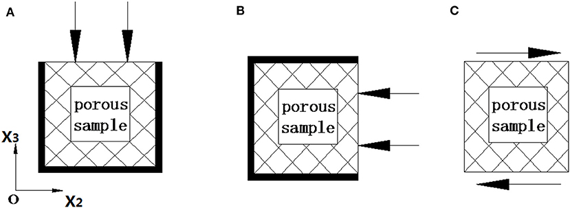
Figure 4. (A–C) Schematic illustration of the three tests adopted to get the corresponding stress–strain relations. The thick bold line represents a zero solid displacement vertical to the edge (Cao et al., 2019). The arrow shows the direction of displacement at the boundary.
In this work, for each test (Figure 4) with specified boundary conditions, the stress–strain relation (Equation D-2) is solved based on the finite-element method (FEM). Detailed information on the process can be found in Appendix D.
A cost function based on the three sets of stress–strain relations could be used to determine the equivalent stiffness tensors (six unknowns) by using the least square method. Details describing the process can be found in the publication reported by Rubino et al. (2016).
Two-Dimensional NIA Solution
According to the NIA theory, the effective elastic compliance tensor S of a cracked medium is determined by two additive components: the compliance tensor of the background medium (Sb) and that of the cracks (ΔS).
where the crack compliance tensor ΔS represents the accumulative contributions of the fractures to the effective compliance tensors, which is a function of the Eshelby (1957) tensors:
where φ represents the crack porosity, J is the fourth-order symmetric identity tensor, Si are the compliance tensors of the individual fractures, and Sbcorresponds to the tensors of host matrix surrounding the fractures, respectively; the components SEshelby represents the Eshelby tensor (Eshelby, 1957; Guo et al., 2019).
For the 2D case, the ellipsoidal fracture inside the volume could be treated as an infinite cylinder (a3 → ∞); therefore, we have the Eshelby tensors in Appendix B (Masson and Pride, 2014). Therefore, the input parameters include the tensors of the host matrix Sb, semiaxis of the fractures, fracture orientations, Poisson ratio, and so on.
In order to get the compliant tensors, a series of parameters are input in advance, including the host matrix Sb; all fracture apertures are assumed to be 3 mm; and the fracture length and the fracture number for two orthogonal fractures are selected by using ant colony algorithms.
The NIA, considering no stress interactions, works well-under the dilute assumption of crack densities. Moreover, according to equation (6), there is no parameter describing the fracture spatial distribution or fracture size distribution; therefore, it could not provide detailed information about fracture clustering.
Evaluation of the Stress Interactions
According to Hudson's theory (Hudson et al., 1996), the effective stiffness tensors of the medium are composed of three parts:
where the summation of the first and second terms corresponds to the inverse matrix of SNIA (equation 6), while the third term ΔΔC is the result of the stress interaction between different fractures. C equals the CNUM (Equation D-2), which could be obtained through the numerical simulation directly. Therefore, a comparison between the and CNUM, allows for the quantification of the effect of stress interactions.
Numerical Results
In this part, a series of fractured models are introduced, with various spatial and length distributions. The corresponding elasticity and anisotropic parameters, affected by the stress interactions, are then studied using the FEM, respectively. Finally, assuming the orthotropy of the fracture clustering, we get the two sets of inverted fracture parameters3.
Fracture Parameter Setup
For a better illustration of the considered fracture networks, we vary the fracture density (e), fracture size distribution (a in equation 1), and aspect ratio (Ξ in Figure 1A) of the fracture clustering. For each parameter combination, 20 stochastic fracture networks are generated. Three typical examples are presented in Figure 5.
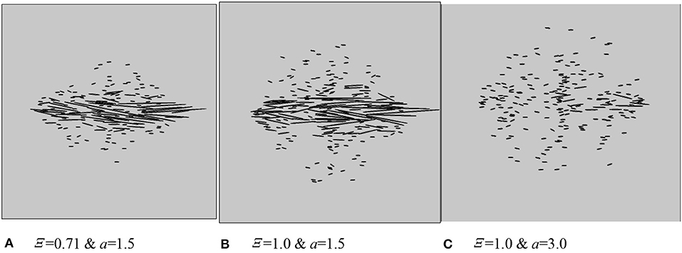
Figure 5. Three different fractured models with various length distributions (A) and spatial distributions (Ξ). The relating characteristic exponent a and the aspect ratio Ξ are given at the bottom of each plot. (A) Ξ = 0.71 & a = 1.5; (B) Ξ = 1.0 & a = 1.5; (C) Ξ = 1.0 & a = 3.0.
For each of the fracture densities (Table 2), a series of numerical models with a given fracture density is presented, with the fracture centers located in different areas for each model (Figure 5).

Table 2. Fracture densities for eight cases with various values of a.
We choose the hypothetical dry sample with isotropic background medium, which has the following parameters: λ = 7.83 GPa; μ = 19.74 GPa (Guo et al., 2019). Moreover, the filling material is the gas whose Young's modulus is 0.066 GPa and the Poisson ratio υ = 0. Additionally, the definition of the fracture density in the 2D sample is introduced as follows:
where n defines the total fracture number inside the 2D sample, r is the major radius of the elliptical 2D fracture, and A is the area of the sample (Guo et al., 2018). Detailed information about the fracture densities for different cases is listed in Table 2.
Effective Elasticity Affected by Stress Interactions
To gain insight into the dominant stress interactions in the fracture clustering, the elastic NIA modulus (Equations B-1, B-2), which neglects stress interactions, is used to compare with the numerical results considering the stress interaction, the gap between them allows for a quantitative description of the dominant stress interactions.
For C33, opposite signs of the gaps between the NIA and the numerical results can be obtained for both long fractures (a = 1.5 in Figure 6A) and short fractures (a = 3.0 in Figure 6B), implying different dominant stress interactions determined by the fracture size. For instance, a smaller C33 produced by NIA compared with the numerical one implies a dominant amplification effect, as given in Figure 6A, while a greater C33 obtained from NIA suggests a weakly dominant shielding effect for case b (Figure 6B; Cao et al., 2020b). Similar rules could also be applied to the shear modulus C44 in Figure 7.
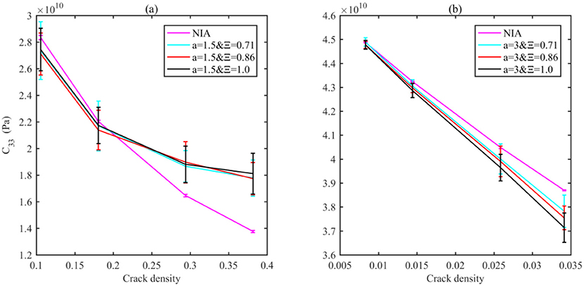
Figure 6. C33 as the functions of fracture densities for different models determined by a and Ξ, using the NIA solution and the numerical method. The lengths of bars are the standard deviations for 20 different realizations by changing the crack locations with the same crack density.
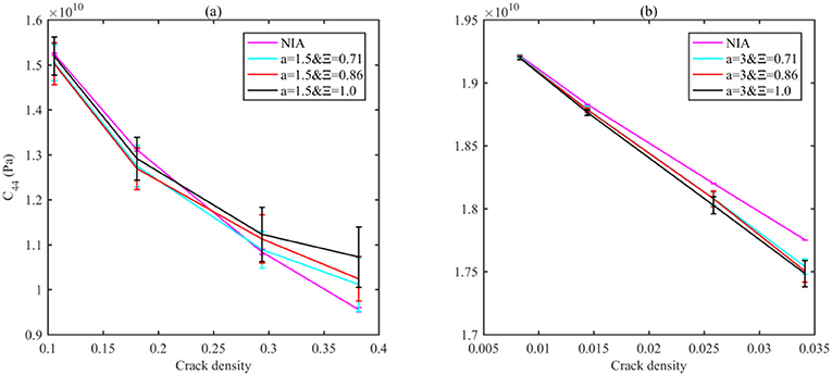
Figure 7. C44 as the functions of fracture densities for different models determined by a and Ξ, using the NIA solution and the numerical method. The numerical result bars are in line with those in Figures 5, 6.
Moreover, modulus discrepancies between different models with various aspect ratios (Ξ) of the bounding ellipsoid are quite different for C33. In Figure 6A, the discrepancies for C33 with different Ξ are negligible for long fractures but more significant for short fractures (a = 3.0 in Figure 6B). Conversely, C44 with various Ξ is greater for long fractures but almost negligible for short fractures.
This can be explained by the effect of the fracture interactions. For long fractures, it is believed that a smaller aspect ratio (Ξ) leads to a smaller distance between the fracture surfaces, which thus leads to a greater shielding effect, especially for the models containing long fractures. However, for the fracture clustering in this study, most of the long fractures concentrate at the core part, and therefore, Ξ variation contributes little to the distance between the close fracture, and thus, the additional shielding effect due to the increment in Ξ is comparably negligible. For short fracture, due to the cancellation of stress interactions (Kachanov, 1993), the net effect of stress interaction is small, and therefore, the additional stress interaction caused by a small variation in Ξ will lead to a more significant change in C33. On the other side, for the shear test (Figure 4C), the shear stress distribution is quite different from the compressive stress in the compressive test (Figures 4A,B; Cao et al., 2020a); it is more than a function of the distance between the ajacent fracture surface; further exploration is expected in the future.
Anisotropic Properties
Besides the effective stiffness tensors (C44 and C33), the anisotropic properties of the fractured samples (Figure 5) could be described by ε and δ. For orthorhombic media, the velocity anisotropic parameters in the 2D can be computed according to equations C-1, C-2.
For the models with long fractures (a = 1.5 in Figure 8A), the shielding effect corresponds to a larger C33. Meanwhile, since the fractures are almost parallel with the X-axis, variation in C22 due to the stress interaction is negligible. Therefore, the stress interaction minimizes the contrast between C22 and C33, corresponding to a decreasing ε, according to equation C-1.
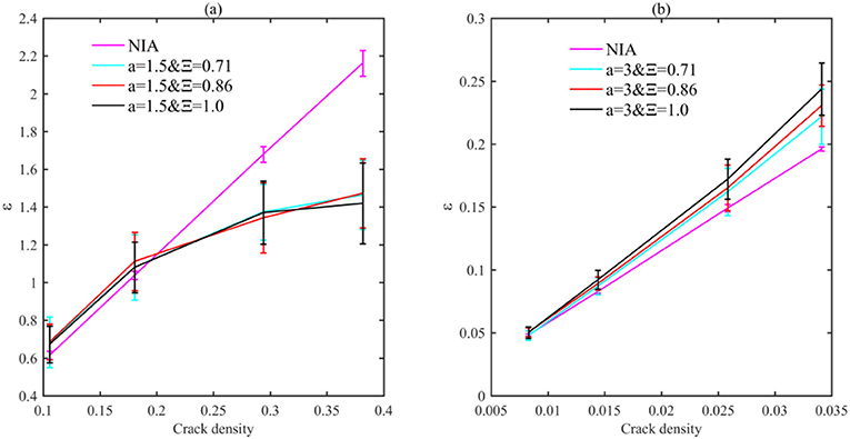
Figure 8. Anisotropic parameters ε, as the function of fracture density, are presented for various rock samples. The bar centers correspond to the averaged values of the numerical ε; the bar sizes define their standard deviations. In the legend, Ξ is the aspect ratio for the ellipse boundary of the fracture clustering, while a = 1.5 (A) and 3 (B) correspond to long and short fractures, respectively. The numerical result bars are in line with those in Figure 6.
However, for ε in the models with short fractures (a = 3 in Figure 8B), similar discrepancies could be observed, but in a reverse pattern, that is, the numerical result is greater than the NIA result. This is understandable since the dominant amplification effect leads to a smaller C33 (Figure 6B).
According to the definition of δ by Woodruff et al. (2015), δ means the difference between the short-offset velocity and the vertical velocity. For the model containing long fractures, the vertical velocity, mainly determined by the shielding effect, leads to a hardening effect that compensates for the shrinking elasticity due to the individual fracture, corresponding to a smaller gap between the short-offset velocity and vertical velocity, which, in turn, leads to a smaller δ in Figure 9A. Furthermore, a greater Ξ means a less dense fracture clustering, and thus a weaker shielding effect, corresponding to a greater δ in Figure 9B.
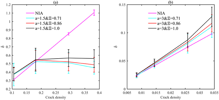
Figure 9. Anisotropic parameters δ, as the function of fracture density, are presented for various rock samples. The centers of the bars correspond to the averaged numerical anisotropic parameter. The numerical result bars are in line with those in Figure 6. In the legend, Ξ is the aspect ratio for the ellipse boundary of the fracture clustering, while a = 1.5 (A) and 3 (B) correspond to the long and short fractures, respectively.
In contrast to the model with long fractures, δ for the model containing short fractures is greater compared with the NIA solution (Figure 9B), due to the dominant amplification effect.
Inversion for Fracture Parameters
Actually, a model containing multiple sets of vertical dry fractures in an isotropic background matrix behaves more like orthotropic media, suggesting that the accumulative contribution of variously oriented fractures to the effective elastic properties is equivalent to that of only two principal fracture sets (Lapin et al., 2018). However, previous publications focused on the application of the approximation in the randomly located models where the net stress interaction is negligible (Grechka and Kachanov, 2006a, Grechka and Kachanov, 2006b; Lapin et al., 2018). As for the damage zone with significant stress interaction, the effects of two types of stress interactions on the effective fracture densities for the two orthogonal sets have not been fully explored yet. We first evaluate the incidence angle dependence of the seismic velocity, so as to check the accuracy of the inverted result. Then, the fracture densities, ex and ey, associated with these two principle fracture sets are inverted from the effective elasticity.
Inversion Methodology
The problem of characterizing multiple fractures has been studied extensively by Grechka and Tsvankin (2003) and Grechka (2007). Using 2D NIA, the authors of the previous publications observed that the accumulative effect of variously oriented fractures on the effective elasticity approaches that of just two orthogonal sets of fractures. Thus, we prefer to employ the NIA solution (Appendix B) to invert the equivalent orthogonal fracture parameters for two orthogonal fractures.
where the unknown vector for fracture characterization contains four parameters:
where n is the fracture number while r is the radius of the fracture; the subscripts x and y refer to the principal axes of a 2D Cartesian coordinate system. In accordance with equation 8, ex and ey for the two orthogonal fracture sets can be predicted based on the assumed orthorhombic effective elasticity.
Based on the stiffness tensors through the numerical solution (Figures 6, 7), we adopt the 2D NIA to compute for a trial vector . Using the ant colony algorithm, we could get the expected fracture parameters, which could minimize the discrepancies (Equation 11) between the trial result and the numerical result. Based on the unknowns in the vector ., the fracture density could be deduced according to equation 6. Detailed information about the inversion procedure is displayed in Figure 10.
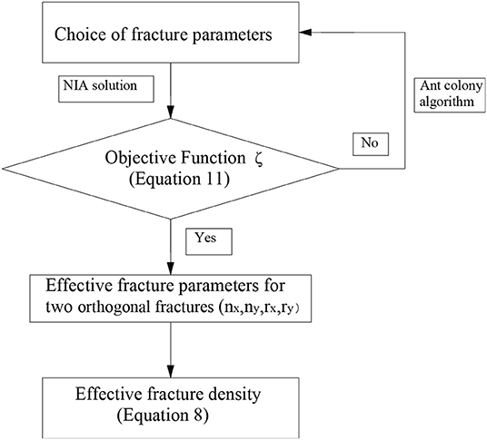
Figure 10. A workflow chart to describe the inversion procedure.
Besides, in NIA, the fracture densities for two sets of orthorhombic fractures could also be obtained directly like the eigenvalues of the second-order fracture–density tensor estimated in equation 9.
The difference between the two types of fracture densities lies in that, both densities fit well with each other under the dilute fracture density assumption. However, at high fracture densities, the two densities will be quite different due to the stress interactions, which also allow for a quantitative description of the stress interaction on the inverted fracture densities.
Incidence Angle Dependence of the Inverted Seismic Velocity
So far, the inversion methodology based on the orthorhombic assumption for fracture clustering has been displayed. In the following, by employing the inverted fracture parameters (Equation 8), the comparability of the inverted result through the incidence angle dependence of the seismic wave is to be checked.
The inverted P- and SV-wave velocities, as functions of the inverted parameters for the two equivalent sets of fractures (blue solid/dashed lines in Figure 11), fit well with the numerical seismic velocities based on the real fracture parameters (Equation A1–A4), suggesting that the inverted parameters obtained are reasonable and that, as expected, the accuracy of the orthorhombic approximation is acceptable.
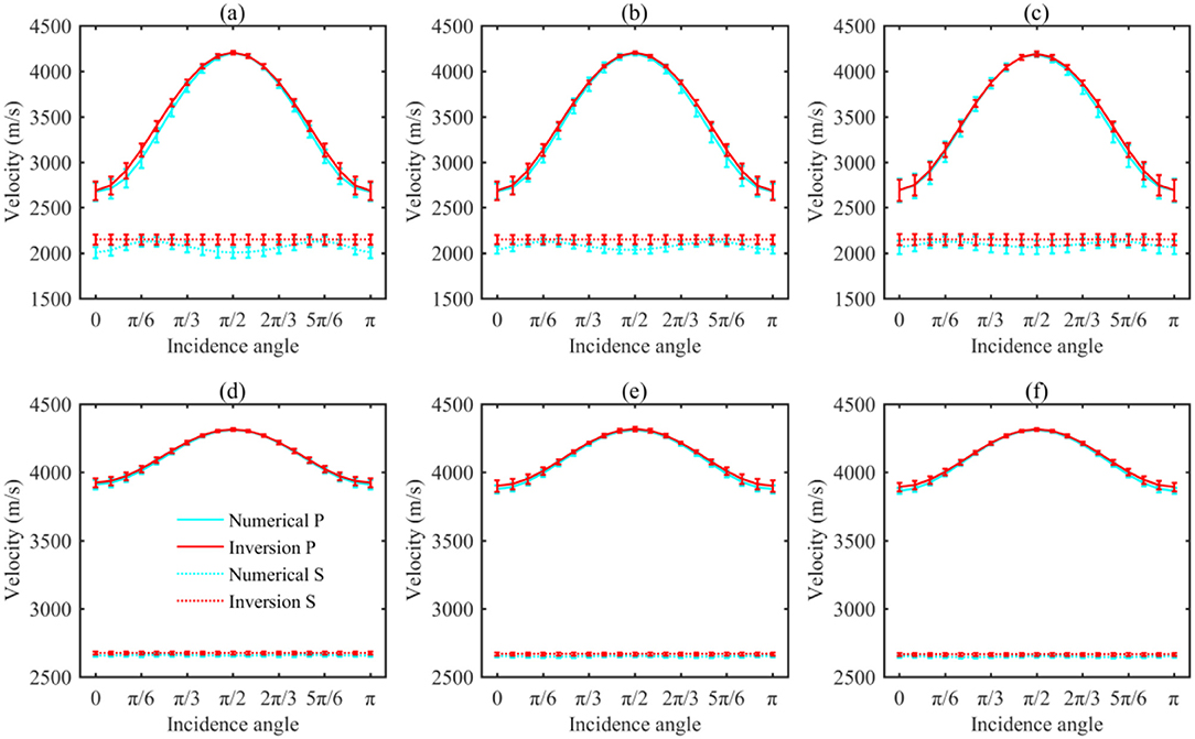
Figure 11. P-wave (solid lines) and SV-wave (dashed lines) velocities as functions of different incidence angles for six kinds of models. (A) a = 1.5, Ξ = 0.71; (B) a = 1.5, Ξ = 0.86; (C) a = 1.5, Ξ = 1; (D) a = 3, Ξ = 0.71; (E) a = 3, Ξ = 0.86; (F) a = 3, Ξ = 1. The blue line denotes the results obtained from the numerical simulations, which is based on the real fracture parameters, while the red line represents the results obtained from NIA, but using the inverted fracture parameters.
However, some minor gaps in the magnitude of the SV-wave anisotropy exist, especially for the case with long fractures (Figure 11A). These are expected for the following reasons: for long fractures (a = 1.5, Figures 11A–C), the medium is the one with the triclinic system, and thus, the nonzero C24 and C34 (Equation 5), due to the stress interactions, lead to greater SV-wave fluctuations.
Effect of Stress Interactions on the Inverted Fracture Densities
Considering the good agreement between the numerical velocities and the inverted data (Figure 11), the authors would like to further explore the effect of stress interactions on the inverted fracture parameters.
For long fractures (a = 1.5 in Figure 12A), the inverted ey is gradually biased toward the smaller values, especially at the high fracture densities, where the relative error reaches nearly 50%. A similar bias that was observed by Grechka and Kachanov (2006b) corresponds to the hardening effect of the shielding effect. On the other side, for short fractures (a = 3 in Figure 12B), the greater slope of the inverted fracture density ey (solid lines) suggests a slightly dominant amplification effect of fracture interactions, whose relative error is about 10%, which is much smaller compared with that of the long fracture.
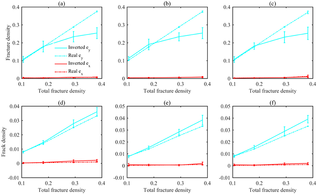
Figure 12. Principal fracture densities ex and ey for different models. (A) a = 1.5, Ξ = 0.71; (B) a = 1.5, Ξ = 0.86; (C) a = 1.5, Ξ = 1; (D) a = 3, Ξ = 0.71; (E) a = 3, Ξ = 0.86; (F) a = 3, Ξ = 1. The solid line corresponds to the inverted result. The numerical result bars are in line with those in Figure 6. The dashed line corresponds to ex and ey predicted as eigenvalues of the density tensor illustrated by Equation 10.
Moreover, for both long (Figures 12A–C) and short fractures (Figures 12D–F), similar gaps between the blue solid and blue dashed lines for the models with various Ξ suggest that aspect ratio (Ξ) contributes little to inverted fracture densities.
On the other hand, for the wave propagates along with the fracture surface, the effect of stress interaction is negligible; therefore, the inverted fracture density ex has an overall agreement with the NIA ones generally.
Actually, the inverted fracture densities based on NIA share the same size, which, however, bias the real models with various length scales and spatial distributions. Furthermore, due to the limitation of the NIA solution, the inverted result could not provide information about the spatial distribution of fractures.
Discussions
According to many previous publications about the T-matrix method (Jakobsen, 2012, Jakobsen and Chapman, 2009), the aspect ratio (Ξ) characterizing the spatial distribution of fractures (Jakobsen et al., 2003, Zhao et al., 2015) represents the conditional probability of finding another inclusion given the position of a known inclusion. However, the definition of such a parameter limits its application in describing fracture clustering. In the present work, the aspect ratio is used to characterize the boundary of the fracture clustering. Such a definition change for the aspect ratio (Ξ) allows for the description of the properties for the fracture clustering.
According to Lapin et al. (2018), for the NIA, the effective elastic properties of an isotropic matrix with fractures distributed in certain spatial patterns always possess the orthorhombic symmetry, regardless of the orientations of the fractures without the same symmetry. However, due to the effect of stress interactions, the model behaves like a triclinic medium rather than an orthorhombic one. Thus, the nonzero moduli C24 and C34, due to the stress interaction, contribute more to the SV-wave anisotropy, leading to more obvious SV-wave velocity fluctuation (such as the SV-wave velocity in Figure 11A).
Both the fracture size and the aspect ratio of the fracture cluster contribute to the effective elasticity. However, an agreement between C33 for the models with various aspect ratios suggests that the contribution of aspect ratio to the stress interaction is negligible, partly due to the fact that variation in the aspect ratio influences the distance between the short fractures distributed at the outer part of the damage zone more when compared to the long fractures at the core part.
It should be noted that all the fractures inside the cluster have no intersection with each other, which, however, is counterintuitive to reality. Nonetheless, according to the conclusion of Grechka and Kachanov (2006b), the fracture intersections impose negligible influence on the effective tensors. Therefore, the conclusion presented in this study still holds acceptable accuracy for the fractured clustering in the field.
Garboczi and Berryman (2001) believe that the error of the numerical simulation may come from statistical variation due to the inhomogeneous distribution of fractures. For the inhomogeneous distribution with a given concentration of cracks, there are multiple spatial arrangements for the cracks, which may have somewhat different elastic moduli. The error size due to inhomogeneous distribution could be assessed by computing the elastic parameters for various realizations of the same system. Therefore, all numerical results as well as the inverted parameters are determined based on the 20 different realizations by changing the crack locations with the same crack density, which could guarantee the accuracy of the conclusions in this study.
Throughout the article, the fracture aperture is set to be 3 mm. However, the aperture varies a lot in the field, which would also contribute to the effect of stress interactions. According to current knowledge, the aperture will also affect both types of stress interactions; further development in this aspect is expected in the future.
Conclusion
Aiming at the damage zone in the fault, numerical models based on the characteristics of the fracture clustering were built, based on which the authors analyzed the effective elastic tensors of the fracturing clusters and estimated the fracture parameters based on the orthorhombic assumption.
Long parallel fractures tend to generate a strong shielding effect, which, therefore, contribute more to the C33 and C44, and a smaller ε. Conversely, the weakly dominant amplification effect induced by the short fractures leads to smaller C33 and C44, and a greater ε. Moreover, the effect of the boundary aspect ratio (Ξ) on the stress interaction for fracture clustering is almost negligible for long fractures (a = 1.5) but relatively more significant for the short fractures (a = 3), where a greater Ξ corresponds to a greater amplification effect.
The inverted fracture density is also strongly influenced by the stress interaction. Amplification tends to weakly overestimate the fracture density while the shielding effect underestimates the fracture density. Furthermore, the incidence angle dependency for the P-wave velocity in fracture clustering is similar to that for the medium containing two orthogonal or principal fracture sets; however, the similarity is somewhat less satisfactory for the SV-wave velocity.
Data Availability Statement
The raw data supporting the conclusions of this article will be made available by the authors, without undue reservation.
Author Contributions
L-YF and CC conceived the research. CC wrote the manuscript and prepares the figures. L-YF reviewed and supervised the manuscript. B-YF and QG are involved in the modeling and inversion programme, respectively. All authors finally approve the manuscript and thus agree to be accountable for this work.
Funding
The Strategic Priority Research Program of the Chinese Academy of Sciences (Grant No. XDA14010303).
Conflict of Interest
The authors declare that the research was conducted in the absence of any commercial or financial relationships that could be construed as a potential conflict of interest.
Supplementary Material
The Supplementary Material for this article can be found online at: https://www.frontiersin.org/articles/10.3389/feart.2021.643372/full#supplementary-material
References
Barbosa, N. D., Rubino, J. G., Caspari, E., and Holliger, K. (2018). Impact of fracture clustering on the seismic signatures of porous rocks containing aligned fracturesFracture clustering effects on WIFF. Geophysics 83:A65–A68. doi: 10.1190/geo2017-0799.1
Bonnet, E., Bour, O., Odling, N. E., Davy, P., Main, I., Cowie, P., et al. (2001). Scaling of fracture systems in geological data. Rev. Geophys. 39, 347–383. doi: 10.1029/1999RG000074
Cao, C., Chen, F., Fu, L.-Y., Ba, J., and Han, T. (2020a). Effect of stress interactions on anisotropic P-SV-wave dispersion and attenuation for closely spaced cracks in saturated porous media. Geophys. Prospect. 68, 2536–2556. doi: 10.1111/1365-2478.13007
Cao, C., Fu, L.-Y., Ba, J., and Zhang, Y. (2019). Frequency- and incident-angle-dependent P-wave properties influenced by dynamic stress interactions in fractured porous media. Geophysics. 84, 1–12. doi: 10.1111/1365-2478.12446
Cao, C., Fu, L.-Y., and Fu, B.-Y. (2020b). An elastic numerical method based on the 3D complex medium. Chin. J. Geophys. 63, 2836–2845. doi: 10.6038/cjg2020N0035
de Dreuzy, J.-R., Davy, P., and Bour, O. (2001). Hydraulic properties of two-dimensional random fracture networks following a power law length distribution: 1. Effective connectivity. Water Res. Res. 37, 2065–2078. doi: 10.1029/2001WR900011
Eshelby, J. D. (1957). The Determination of the elastic field of an ellipsoidal inclusion, and related problems. Proc. R. Soc. Lond. 241, 376–396. doi: 10.1098/rspa.1957.0133
Garboczi, E. J., and Berryman, J. G. (2001). Elastic moduli of a material containing composite inclusions: effective medium theory and finite element computations. Mech. Mater. 33, 455–470. doi: 10.1016/S0167-6636(01)00067-9
Grechka, V. (2007). Multiple cracks in VTI rocks: effective properties and fracture characterization. Geophysics 72, D81–D91. doi: 10.1190/1.2751500
Grechka, V., and Kachanov, M. (2006a). Effective elasticity of fractured rocks: a snapshot of the work in progress. Geophysics 71, W45–W58. doi: 10.1190/1.2360212
Grechka, V., and Kachanov, M. (2006b). Effective elasticity of rocks with closely spaced and intersecting cracks. Geophysics 71, D85–D91. doi: 10.1190/1.2197489
Grechka, V., and Tsvankin, I. (2003). Feasibility of seismic characterization of multiple fracture sets. Geophysics 68, 1399–1407. doi: 10.1190/1.1598133
Guo, J., Han, T., Fu, L., Xu, D., and Fang, X. (2019). Effective elastic properties of rocks with transversely isotropic background permeated by aligned penny-shaped cracks. J. Geophys. Res. Solid Earth 124, 400–424. doi: 10.1029/2018JB016412
Guo, J., Rubino, J. G., Barbosa, N. D., Glubokovskikh, S., and Gurevich, B. (2018). Seismic dispersion and attenuation in saturated porous rocks with aligned fractures of finite thickness: theory and numerical simulations — part 1: P-wave perpendicular to the fracture plane. Geophysics 83, WA49–WA62. doi: 10.1190/geo2017-0065.1
Harris, S., McAllister, E., Knipe, R., and Odling, N. E. (2003). Predicting the three-dimensional population characteristics of fault zones: a study using stochastic models. J. Struct. Geol. 25, 1281–1299. doi: 10.1016/S0191-8141(02)00158-X
Hopkins, D. L. (2000). The implications of joint deformation in analyzing the properties and behavior of fractured rock masses, underground excavations, and faults. Int. J. Rock Mech. Min. Sci. 37, 175–202. doi: 10.1016/S1365-1609(99)00100-8
Hudson, J. A., Liu, E., and Crampin, S. (1996). The mechanical properties of materials with interconnected cracks and pores. Geophys. J. Int. 124, 105–112. doi: 10.1111/j.1365-246X.1996.tb06355.x
Hunziker, J., Favino, M., Caspari, E., Quintal, B., Rubino, J. G., Krause, R., et al. (2018). Seismic attenuation and stiffness modulus dispersion in porous rocks containing stochastic fracture networks. J. Geophys. Res. Solid Earth 123, 125–143. doi: 10.1002/2017JB014566
Jakobsen, M. (2012). T-matrix approach to seismic forward modelling in the acoustic approximation. Stud. Geophys. Et Geodaet. 56, 1–20. doi: 10.1007/s11200-010-9081-2
Jakobsen, M., and Chapman, M. (2009). Unified theory of global flow and squirt flow in cracked porous media. Geophysics 74, WA65–WA76. doi: 10.1190/1.3078404
Jakobsen, M., Hudson, J. A., and Johansen, T. A. (2003). T-matrix approach to shale acoustics Geophys. J. Int. 154, 533–558. doi: 10.1046/j.1365-246X.2003.01977.x
Kachanov, M. (1993). Elastic solids with many cracks and related problems. Adv. Appl. Mech. 30, 259–445. doi: 10.1016/S0065-2156(08)70176-5
Lapin, R., Kuzkin, V., and Kachanov, M. (2018). On the anisotropy of cracked solids. Int. J. Eng. Sci. 124, 16–23. doi: 10.1016/j.ijengsci.2017.11.023
Lei, Q., and Gao, K. (2018). Correlation between fracture network properties and stress variability in geological media. Geophys. Res. Lett. 45, 3994–4006. doi: 10.1002/2018GL077548
Masson, Y. J., and Pride, S. R. (2007). Poroelastic finite difference modeling of seismic attenuation and dispersion due to mesoscopic-scale heterogeneity. J. Geophys. Res. Atmosph. 112, 1642–1642. doi: 10.1029/2006JB004592
Masson, Y. J., and Pride, S. R. (2014). On the correlation between material structure and seismic attenuation anisotropy in porous media. J. Geophys. Res. Solid Earth 119, 2848–2870. doi: 10.1002/2013JB010798
Mavko, G., Mukerji, T., and Dvorkin, J. (2009). The Rock Physics Handbook, 2nd Edn. Cambridge: Cambridge University Press.
Odling, N., Harris, S., Vaszi, A., and Knipe, R. (2005). Properties of fault damage zones in siliclastic rocks: a modelling approach. Geolog. Soc. Lond. 249, 43–59. doi: 10.1144/GSL.SP.2005.249.01.04
Quintal, B., Steeb, H., Frehner, M., and Schmalholz, S. (2011). Quasi-static finite element modeling of seismic attenuation and dispersion due to wave-induced fluid flow in poroelastic media. J. Geophys. Res. 116:B01201. doi: 10.1029/2010JB007475
Quintal, B., Steeb, H., Frehner, M., Schmalholz, S. M., and Saenger, E. H. (2012). Pore fluid effects on S-wave attenuation caused by wave-induced fluid flow. Geophysics 77, L13–L23. doi: 10.1190/geo2011-0233.1
Rubino, J. G., Caspari, E., Müller, T. M., Milani, M., Barbosa, N. D., and Holliger, K. (2016). Numerical upscaling in 2-D heterogeneous poroelastic rocks: Anisotropic attenuation and dispersion of seismic waves. J. Geophys. Res. Solid Earth 121, 6698–6721. doi: 10.1002/2016JB013165
Savage, H., and Brodsky, E. (2011). Collateral damage: Evolution with displacement of fracture distribution and secondary fault strands in fault damage zones. J. Geophys. Res. 116:B03405. doi: 10.1029/2010JB007665
Schoenberg, M., and Sayers, C. (1995). Seismic anisotropy of fracture rock. Geophysics 60, 204–211. doi: 10.1190/1.1443748
Wenzlau, F., Altmann, J. B., and Müller, T. M. (2010). Anisotropic dispersion and attenuation due to wave-induced fluid flow: Quasi-static finite element modeling in poroelastic solids. J. Geophys. Res. 115:B07204. doi: 10.1029/2009JB006644
Woodruff, W. F., Revil, A., Prasad, M., and Torres-Verdín, C. (2015). Measurements of elastic and electrical properties of an unconventional organic shale under differential loading. Geophysics 80, D363–D383. doi: 10.1190/geo2014-0535.1
Keywords: stress interaction, fracture clustering, damage zone, inversion, modeling
Citation: Cao C, Fu L-Y, Fu B-Y and Guo Q (2021) Effect of Stress Interactions on Effective Elasticity and Fracture Parameters in the Damage Zones. Front. Earth Sci. 9:643372. doi: 10.3389/feart.2021.643372
Received: 18 December 2020; Accepted: 21 April 2021;
Published: 13 May 2021.
Edited by:
Pascal Audet, University of Ottawa, CanadaReviewed by:
Ke Gao, Southern University of Science and Technology, ChinaJunxin Guo, Southern University of Science and Technology, China
Copyright © 2021 Cao, Fu, Fu and Guo. This is an open-access article distributed under the terms of the Creative Commons Attribution License (CC BY). The use, distribution or reproduction in other forums is permitted, provided the original author(s) and the copyright owner(s) are credited and that the original publication in this journal is cited, in accordance with accepted academic practice. No use, distribution or reproduction is permitted which does not comply with these terms.
*Correspondence: Li-Yun Fu, bGZ1QHVwYy5lZHUuY24=