Fracture Shape and Orientation Contributions to P-Wave Velocity and Anisotropy of Alpine Fault Mylonites

P-wave anisotropy is significant in the mylonitic Alpine Fault shear zone. Mineral- and texture-induced anisotropy are dominant in these rocks but further complicated by the presence of fractures. Electron back-scattered diffraction and synchrotron X-ray microtomography (micro-CT) data are acquired on exhumed schist, protomylonite, mylonite, and ultramylonite samples to quantify mineral phases, crystal preferred orientations, microfractures, and porosity. The samples are composed of quartz, plagioclase, mica and accessory garnet, and contain 3–5% porosity. Based on the micro-CT data, the representative pore shape has an aspect ratio of 5:2:1. Two numerical models are compared to calculate the velocity of fractured rocks: a 2D wave propagation model, and a differential effective medium model (3D). The results from both models have comparable pore-free fast and slow velocities of 6.5 and 5.5 km/s, respectively. Introducing 5% fractures with 5:2:1 aspect ratio, oriented with the longest axes parallel to foliation decreases these velocities to 6.3 and 5.0 km/s, respectively. Adding both randomly oriented and foliation-parallel fractures hinders the anisotropy increase with fracture volume. The anisotropy becomes independent of porosity when 80% of fractures are randomly oriented. Modeled anisotropy in 2D and 3D are different for similar fracture aspect ratios, being 30 and 15%, respectively. This discrepancy is the result of the underlying assumptions and limitations. Our numerical results explain the effects that fracture orientations and shapes have on previously published field- and laboratory-based studies. Through this numerical study, we show how mica-dominated, pore-free P-wave anisotropy compares to that of fracture volume, shape and orientation for protolith and shear zone rocks of the Alpine Fault.

1. Introduction

The Alpine Fault is located along the West Coast of the South Island, New Zealand. It marks the transpressional plate boundary between the Australian and the Pacific Plates (Figure 1). The fault hosts many earthquakes a year, but a large earthquake (M_w > 7.0) occurs every <300 years on average with the last one occurring in 1717 AD (Sutherland et al., 2007; Howarth et al., 2018). The majority of the rocks on the Pacific Plate (hanging wall) are schist and fault rocks. Rocks sheared during the collision of the two plates form a series of fault rocks close to the principal slip zone consisting of fault gouge, cataclasite, and variable grades of mylonites which vary according to fault-perpendicular distance. Mylonites do not outcrop in the footwall, but the hanging wall mylonite zone is approximately 1 km thick (Norris and Cooper, 1997). The mylonites are derived from the Alpine Schist and developed foliation parallel and sub-parallel to the fault plane (Toy et al., 2008). In general, the mylonites and schist are composed of quartz, plagioclase, biotite, muscovite, and accessory minerals such as chlorite, garnet, and calcite (Grapes and Watanabe, 1994; Little et al., 2002; Toy et al., 2015; Boulton et al., 2017).

FIGURE 1

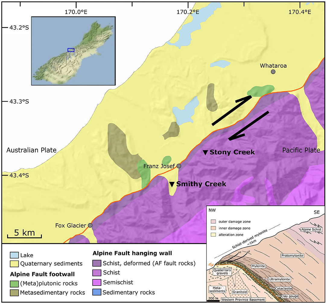
Figure 1. Simplified geological map of the study area and cross-section showing typical shallow-depth sequence of the Alpine Fault rocks (Norris and Cooper, 2007; Schuck et al., 2020). Alpine Fault trace shown in orange; Stony Creek and Smithy Creek are indicated by black triangles. Map is based on the geological map of New Zealand's South Island (Edbrooke et al., 2015) and the digital elevation model of Columbus et al. (2011).

Field passive and active source seismic data has been used to investigate the Alpine Fault geometry and rock physical properties. Such data show a low-velocity zone in the hanging wall that lies parallel to the Alpine Fault (Smith et al., 1995; Stern et al., 2001, 2007; Feenstra et al., 2016; Lay et al., 2016). Within the first 10 km depth, the P-wave velocity of the low-velocity zone is 5.5–6.0 km/s compared to the velocity outside the zone of 6.0–6.5 km/s. This low-velocity zone is commonly interpreted to be due to the presence of fluid-filled microfractures, but experimental and model data needed to validate such a claim are rare (Allen et al., 2017; Adam et al., 2020). The fault damage zone has been investigated using fault guided (trapped) seismic wave observation and modeling (Eccles et al., 2015; Kelly et al., 2017). However, these field studies that aim to characterize the fault geometry and physical properties do not account for seismic anisotropy. It is well-known that assuming isotropic seismic velocity models for anisotropic rocks will result in erroneous modeling and interpretations (Chapman and Pratt, 1992; Godfrey et al., 2002; Tsvankin et al., 2010). It is therefore critical to quantify how the physical properties of Alpine Fault rocks influence elastic wave anisotropy.

Previous studies using seismic data (Savage et al., 2007; Karalliyadda and Savage, 2013), core measurements (Okaya et al., 1995; Godfrey et al., 2000; Christensen and Okaya, 2007; Allen et al., 2017; Simpson et al., 2019; Adam et al., 2020; Jeppson and Tobin, 2020) and numerical modeling (Godfrey et al., 2002; Dempsey et al., 2011; Adam et al., 2020; Simpson et al., 2020) demonstrate that the rock in the vicinity of the Alpine Fault is strongly anisotropic. The anisotropy is attributed to many factors such as mineral crystallographic preferred orientation (CPO), grain shape preferred orientation (SPO), foliation and fractures. The Alpine Fault rocks contain significant (>15 vol%) mica with preferred orientation (Dempsey et al., 2011; Adam et al., 2020). Dempsey et al. (2011) has shown how the volume of aligned mica influences P-wave anisotropy in mylonite from the Alpine Fault. Moreover, grain size insensitive creep-accommodated ductile shear resulted in a CPO of quartz and plagioclase as well as their SPO (Toy et al., 2008). Velocity measurements under confining pressure also show directionally, non-uniform changes in P-wave velocities with depth which implies that aligned fractures are present (Adam et al., 2020; Simpson et al., 2020).

Fractures herein are described as flat-shaped pores. Fractures can form within the rock as intergranular spaces between flat-shaped grains in sedimentary rocks (Loucks et al., 2009), or can form as a secondary structures when the rocks are exposed to differential stress (e.g., Pischiutta et al., 2015). In many tectonic scenarios, fractures can develop as an aligned set. These aligned fractures affect the seismic anisotropy of rocks. The fractures can induce seismic anisotropy in an isotropic host rock, or further enhance pre-existing anisotropy (Kern et al., 2008; Novitsky et al., 2018). The degree of fracture-induced seismic anisotropy enhancement depends on many factors such as fracture volume (porosity), orientation, and shape (Hong-Bing et al., 2013; Vasin et al., 2013). These factors should be incorporated into seismic velocity modeling.

Adam et al. (2020) showed that open grain boundaries and microfractures can enhance the seismic wave anisotropy at all depths of the seismogenic zone in the Alpine Fault. Simpson et al. (2020) predict the P-wave anisotropy of shallow Alpine Fault rocks. However, those studies did not systematically consider the effect of mica CPO and shape/orientation of fractures on seismic anisotropy.

Here we quantify fracture shape, mineral phase, and crystal orientations from synchrotron X-ray microtomography data and electron back-scattered diffraction (EBSD) data. Based on these measurements, we model P-wave speeds and anisotropy for a range of Alpine Fault rocks. The effect of fractures on Alpine Fault rocks is modeled using two numerical methods: a wave propagation and a differential effective medium modeling approach. The methods differ in being dynamic and static respectively, as well as in the way that fractures are in 2D and 3D. Our study compares the models and their limitations for the inclusion of mica CPO and distribution, and fractures to predict seismic wave anisotropy.

2. Materials and Methods

2.1. Electron Back-Scattered Diffraction (EBSD)

Rock samples were collected from Central Alpine Fault outcrops which span shear zone mylonites and schist. The schist sample was collected at Smithy Creek and is part of the Alpine Schist tectonostratigraphic unit (Cooper and Palin, 2018). The protomylonite, mylonite and ultramylonite samples are from Stony Creek (Figure 1). Thin sections of 35 μm thickness are prepared for all samples and subjected to fine SYTON polish to be examined using EBSD. Thin sections for the samples are created for two angles to foliation: 90^o (perpendicular to foliation) and 30^o. No pores or fractures are visible in the specimens under optical microscope or in microphotographs.

EBSD experiments are performed to produce a phase map containing mineralogical and crystallographic orientation data. EBSD data were acquired on 2 by 2 mm areas on the thin sections using a Zeiss Sigma VP FE-SEM fitted with an Oxford Instruments HKL INCA Premium Synergy Inte30 grated ED/BSD system, located at the Otago Microscopy and Nano-Imaging (OMNI). The SEM is operated with an accelerating voltage of 30 keV, an aperture size of 300 μm, and a working distance of approximately 30 mm. The EBSD data were acquired at a 2 μm step size then used to quantify mineral phase composition and crystallographic preferred orientation (CPO).

The EBSD data were processed to reduce noise and fill any data gaps using the MTEX toolbox (Mainprice et al., 2015). First, grain boundaries were reconstructed by grouping same-phase mineral data with less than 10^o misorientation angle. Then, all isolated 1-pixel grains were deleted to eliminate wild pixels (i.e., noise). Grain boundaries were reconstructed again using the same criteria as the previous step. Grains with less than 30% indexed fraction were removed. The indexed fraction is a ratio between the area of the indexed pixel in the grain to the whole grain area. Grains smaller than 10 pixels were also removed. Lastly, in-grain pixels were smoothed and filled based on their surrounding pixels using a spline filter.

Fine-grained phyllosilicate minerals, dominant in mylonite rocks, are mostly unable to be indexed by EBSD and appear in the maps as non-indexed phase (Prior and Mariani, 2009; Dempsey et al., 2011; Adam et al., 2020). To improve indexing of mica, we performed EBSD on an additional cut to the samples at 30^o from foliation with the hope to gain surface area on the mica to improve indexing. Unfortunately, we had about the same volume of non-indexed phase as for the 90^o cut to foliation. Toy et al. (2008) and Dempsey et al. (2011) show the smallest phases in the Alpine Fault mylonites are dominantly mica. We therefore assign the non-indexed phases to mica. Moreover, based on photomicrographs and synchrotron micro-CT imaging, mica within Alpine Fault mylonite (Toy et al., 2008; Adam et al., 2020) is parallel and subparallel to foliation. We therefore, assume that most non-indexed phases (i.e., mica) are parallel to foliation and account for the sub-parallel mica in terms of randomly oriented mica. Microfractures and open grain boundaries would also show as non-indexed phases, however, these are mostly not resolved in the EBSD imaging. It is important to understand that the EBSD data does not have information regarding pores or fractures of these rocks. Since all non-indexed pixels are substituted with mica in our models, the effect of microfractures is later included separately in the finite difference and the wave propagation models.

It is clear that not all micas are perfectly parallel to foliation. To determine the mica orientation, we use the P-wave high pressure data from Adam et al. (2020) where most of the fractures are assumed to be closed with a 0.5% modeled porosity to estimate the volumetric contribution of parallel and randomly oriented mica basal plane orientation. We compare MTEX models of fast and slow P-wave velocities based on the combinations of perfectly and randomly aligned fractures volume to the laboratory data (Supplementary Figure 4). We show that model and experimental data match for a 80:20 volume of parallel:random fractures. We therefore, use this volumetric distribution of mica for all of our models.

2.2. Synchrotron X-Ray Micro-Tomography (Micro-CT)

Micro-CT is a non-destructive method used to investigate the 3D internal structure of an object. The shape of rock microfractures can be extracted and these can statistically be analyzed and converted into mathematical shapes. We use such information to model fracture effects on seismic anisotropy with the wave propagation and differential effective medium models.

Micro-CT data used in this study was collected using beamline 20XU at SPring-8, Japan on a 3 mm height and 1 mm diameter cylinder. The sample was mounted on a rotary stage. X-ray beam of 20 keV energy was shone through the sample onto the scintillator which converts X-ray to visible light. The image was then captured by the CMOS camera detector. The process was repeated over 180^o rotation with 0.1^o step size. The sample cross-sections were reconstructed using a convolution back-projection method, producing a stack of gray-scale which then re-scaled to 8-bit gray-scale images. The data resolution is 0.524 μm.

The micro-CT data were processed using the Avizo software. The gray-scale micro-CT images were cropped into an approximately 250-micron cube. The data were smoothed with a first-degree median filter to reduce noise and artifacts. The filter replaces the CT number in a voxel with the median of the 27 neighboring voxels (voxels within a 1-voxel radius of the center voxel). All pores which are smaller than 8 voxels were also removed, and a hole-filling algorithm was used. After that, pore segmentation was performed using a threshold method based on the CT number. Lastly, 3D pores were reconstructed, and the pore dimension and volume fraction were measured. EBSD and micro-CT data were used to model wave speeds in pore-free and fractured mylonites and schist. These data were combined to compare two modeling approaches: wave propagation and GassDEM modeling.

2.3. Wave Propagation Modeling (EWAVE)

Wave propagation modeling is performed using EWAVE Matlab code (Zhong and Frehner, 2018). The code simulates wave propagation through the EBSD data using an explicit finite-difference time-marching model. The model discretizes the input EBSD data into cells and an elastic stiffness tensor (Table 1) is assigned to each cell based on mineralogy and crystallographic orientation. A Ricker wavelet is digitally propagated across the sample by solving a momentum balance equation and Hooke's law. The wave travel time is recorded and the wave velocity is calculated from the width of the EBSD data and the travel time. The fast and slow velocities are determined by propagating waves parallel and perpendicular to rock foliation, respectively. A detailed explanation is provided in Zhong and Frehner (2018). A time snapshot of wave propagation through a medium is shown in Figure 2. The buffer length and wavelength used in this study are 300 and 100 μm, respectively. P-wave anisotropy is calculated as a ratio between the difference between fast and slow velocity, and the average of the two velocities.

TABLE 1

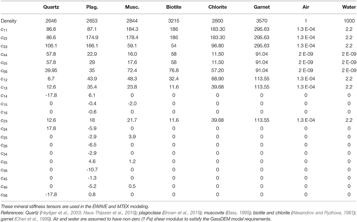
Table 1. Elasticity (in GPa) and density (in kg/m³) of mineral phases present in our samples.

FIGURE 2

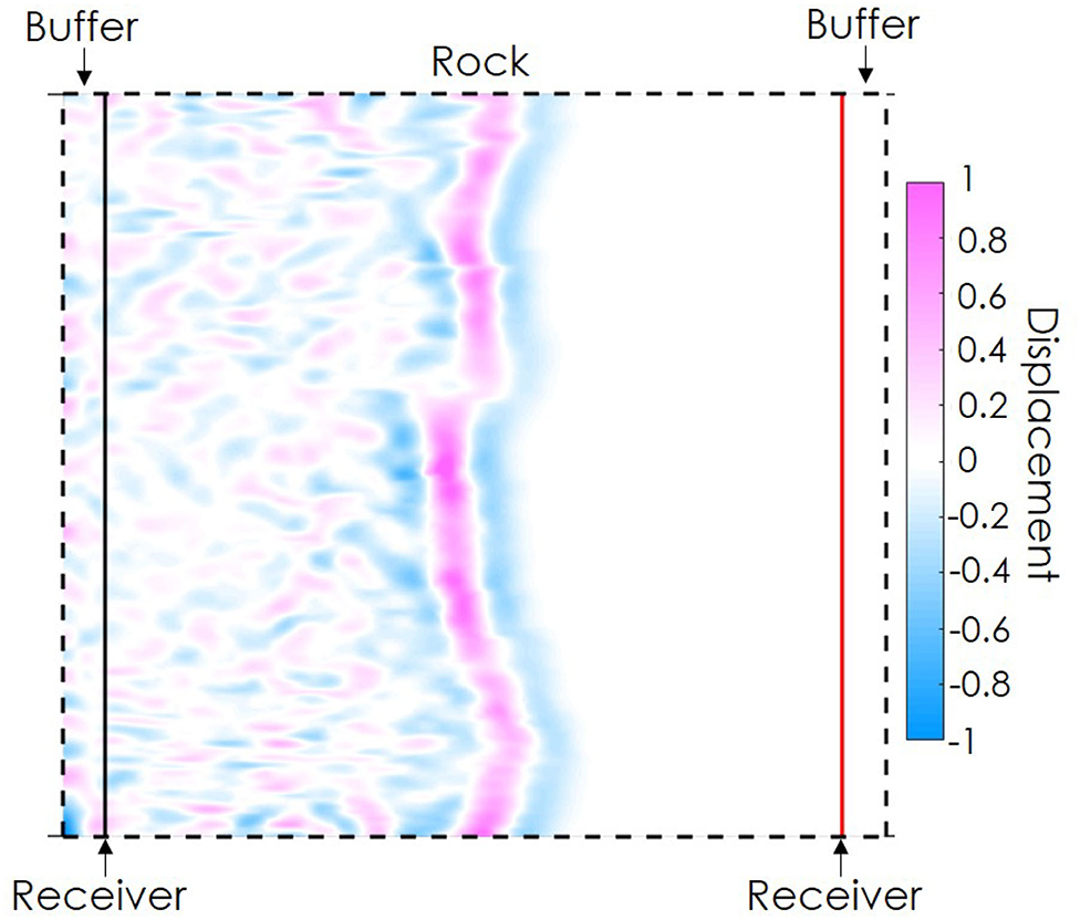
Figure 2. EWAVE model component: EBSD data (“Rock”) is placed between two buffers. A Ricker wave (pink and blue) is propagated from left to right of the model. Two receivers (left: black line, right: red line) are used to record the wave signal and calculate wave travel times. Displacement is dimensionless and does not affect the velocity.

Two types of modeling are performed: (1) a porosity-free EBSD model and (2) the same model but with added fractures defined by specific aspect ratios. EWAVE models EBSD data and could include imaged natural fractures (non-indexed phases) as it propagates a wave through the model (Zhong and Frehner, 2018). However, for our mylonitic rocks, natural fractures were not imaged via EBSD so are not immediately accounted for. We include pore information by extracting natural 3D fracture shapes from micro-CT data. This fracture set is statistically and mathematically simplified into 2D fractures which are deterministically included into the model. These pores are added randomly to the EBSD model at specific aspect ratios parallel to foliation.

2.4. Differential Effective Medium Modeling (MTEX and GassDEM)

A different approach to model the pore-free rock elasticity is by applying the Hill effective medium model implemented in the Matlab MTEX toolbox (Mainprice et al., 2015). The calculation uses the mineral volume fraction and CPO from the EBSD data, together with the single-crystal stiffness tensor of each mineral (Table 1) to predict the whole rock effective stiffness tensor from which wave speeds with direction can be estimated.

To model the effect of pores and fluids on the wave velocities, the pore-free effective stiffness tensor output from MTEX is set as a background rock for GassDEM (Gassmann and DEM) modeling (Kim et al., 2019; Simpson et al., 2020). GassDEM modeling adds fixed aspect ratio inclusions (3D fractures in this case) into the background medium. The process is iterative with additions of small volumes of pores until the target sample porosity is reached (Bruggeman, 1935). Gassmann's equation allows the effect of fluids on the elasticity of the rock to be modeled (Gassmann, 1951; Smith et al., 2003).

We study the effect of fractures on P-wave velocity and anisotropy in two ways: (1) fractures are aligned to foliation and porosity volume is varied and (2) the porosity volume is constant, but the contribution of the fracture orientation is changed for different combinations of aligned and randomly oriented fractures.

3. Results

3.1. Electron Back-Scattered Diffraction (EBSD)

EBSD data show that the shear-zone Alpine Fault rocks are composed of quartz, plagioclase, garnet and a considerable amount of non-indexed phase (Figure 3, Table 2), assumed to be biotite mica as the phyllosilicate minerals in the Alpine Fault mylonites are predominantly biotite (Toy et al., 2015). There is no significant mineralogical difference between the 90^o and 30^o sections nor an improvement of imaging the micas. 80% of the non-indexed mica is assumed to align with foliation and 20% of the non-indexed mica is assumed to be randomly oriented (see section 1.3 in Supplementary Material).

FIGURE 3

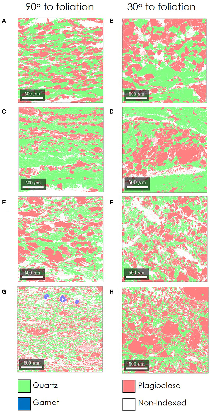
Figure 3. Processed EBSD data of mineral phases distribution of (A,B) schist, (C,D) protomylonite, (E,F) mylonite, and (G,H) ultramylonite cut 90^o and 30^o to foliation, respectively.

TABLE 2

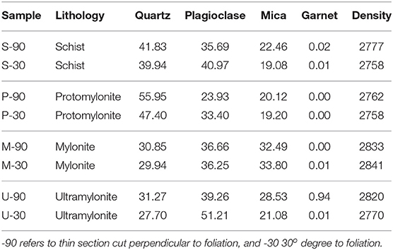
Table 2. Mineral composition (vol.%) and mineral density (kg/m³).

3.2. Synchrotron X-Ray Micro-Tomography (Micro-CT)

Micro-CT data of ultramylonite, mylonite, and protomylonite samples are analyzed to quantify porosity and pore aspect ratio. After pore segmentation is performed (Figure 4), the number of pore voxels is divided by the total number of voxels to calculate porosity. The calculated porosity of ultramylonite, mylonite, and protomylonite are 3.36, 2.08, and 4.88%, respectively. A 5% porosity will be used in the following velocity modeling as it covers all the calculated porosity from the micro-CT data. Pore aspect ratio is measured as a ratio of three orthogonal pore axis lengths (e.g., X:Y:Z where X≥Y≥Z). The three numbers represent the longest axis, the second-longest and the shortest axial length, respectively (Figure 5). Two axial ratios are extracted from the segmented pores: elongation and flatness (Figure 6). Elongation is a ratio between the second-longest and the longest axial length (i.e., Y/X) and flatness is a ratio between the shortest to the second-longest axial length (i.e., Z/Y).

FIGURE 4

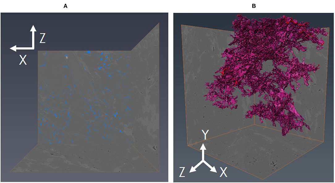
Figure 4. (A) An example of pore segmentation (blue) on a 2D micro-CT slice for a mylonite. (B) The connected 3D pore network (pink) in the sample. The size of the cubic sub-volume of the micro-CT data analyzed and shown here is 470 X 400 X 400 μm³.

FIGURE 5

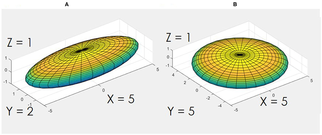
Figure 5. Ellipsoid examples representing fractures of (A) 5:2:1 and (B) 5:5:1 aspect ratio.

FIGURE 6

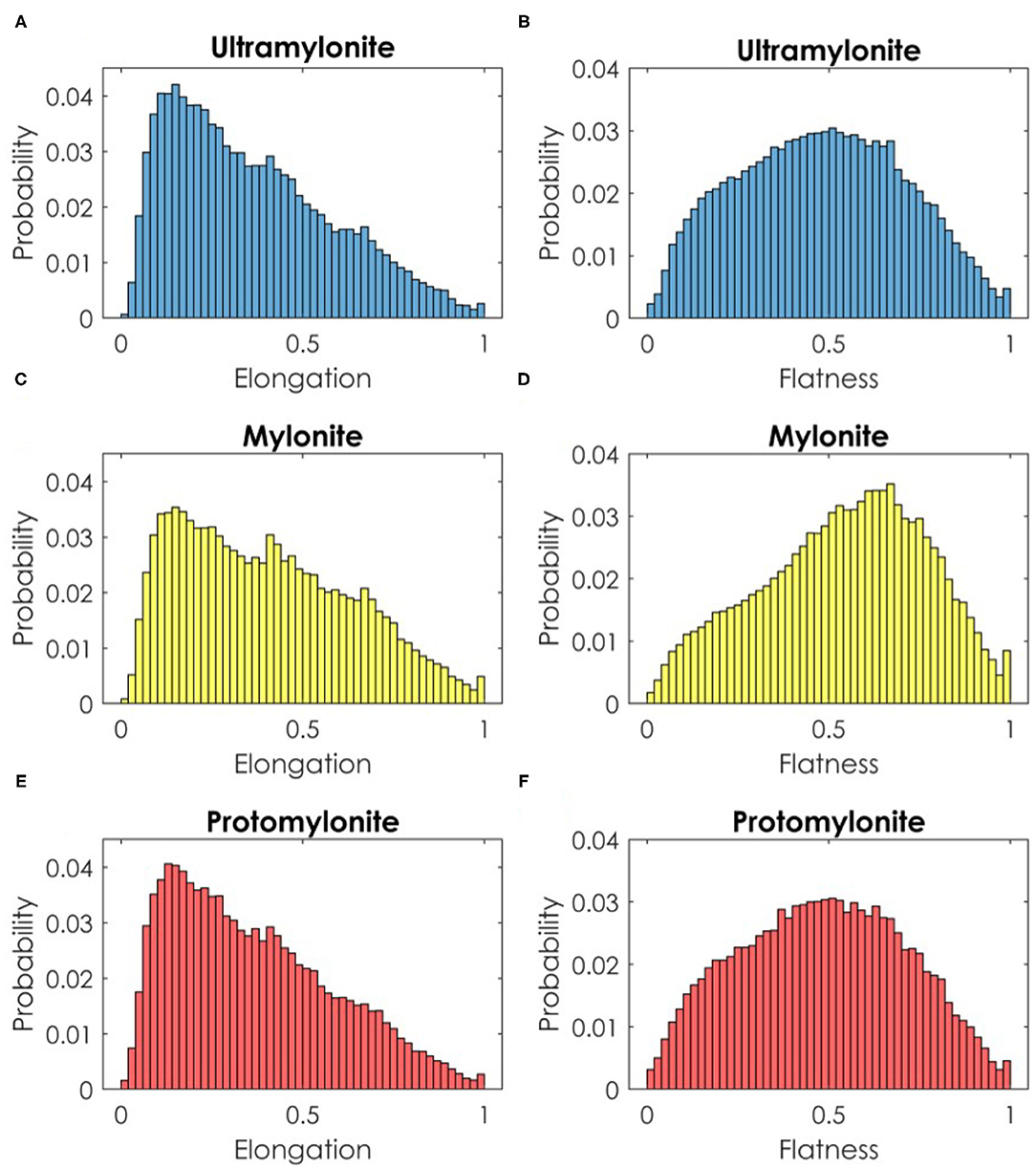
Figure 6. Histograms of pore elongation and flatness in (A,B) ultramylonite, (C,D) mylonite, and (E,F) protomylonite.

The elongation and flatness histogram plots of all three rocks are similar. Elongation plots are right-skewed with mode around 0.16 with the mean and median range from 0.36 to 0.40 and 0.32 to 0.38, respectively. The flatness for the ultramylonite and the protomylonite are almost symmetric with 0.48 mean and median. For the mylonite however, the flatness plot is slightly left-skewed. The mean and median of the mylonite flatness are 0.54 and 0.56, respectively. Pores with small elongation and flatness would represent low aspect ratio fractures, which are thin, long and narrow. Pores with elongation and flatness close to 1 represent close-to-spherical pores. Based on the histogram analysis, the average pore aspect ratio determined from the mean flatness and elongation is 5:2:1. This fracture shape is defined as a flat-shaped pore (fracture) and used for the following P-wave velocity modeling.

3.3. Wave Propagation Modeling (EWAVE)

Fast and slow P-wave velocities are modeled using the EWAVE code. Fracture porosity is added randomly as a 2D projection of the extracted micro-CT fractures of aspect ratio 5:2:1 (Figure 7). Fractures are added with their long-axis parallel to foliation as rectangles of aspect ratio 5:1. For this study, fractures are added by randomly replacing pixels in the EBSD data with air/water. The influence of fracture porosity volume is studied by adding fractures in 1% increments up to a total porosity of 5%. In this modeling, pores are dry (filled with air). For such low porosity, modeling air- or water-filled fractures results in a velocity difference of less than 2% of the air-filled fracture model. The pore-free fast velocities are similar for all rocks at 6.5 km/s, while the slow velocities range from 5.5 to 6.0 km/s depending on the lithology (Figure 8A). As porosity is added to the model, both fast and slow velocities decrease linearly. The fast velocities decrease slightly to 6.3 km/s at 5% porosity. The slow velocities however, decrease rapidly to 4.5 km/s. The P-wave anisotropy is also calculated (Figure 8C), ranging from 10 to 15% and increasing linearly to 30–35% for a 5 % fracture porosity.

FIGURE 7

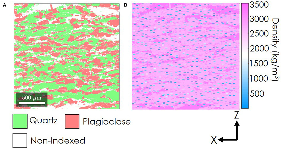
Figure 7. (A) Schist EBSD data cut perpendicular to foliation and (B) the EWAVE model of the schist data with 5% fractures included. The color represents the phase density. The air-filled fractures are shown in blue.

FIGURE 8

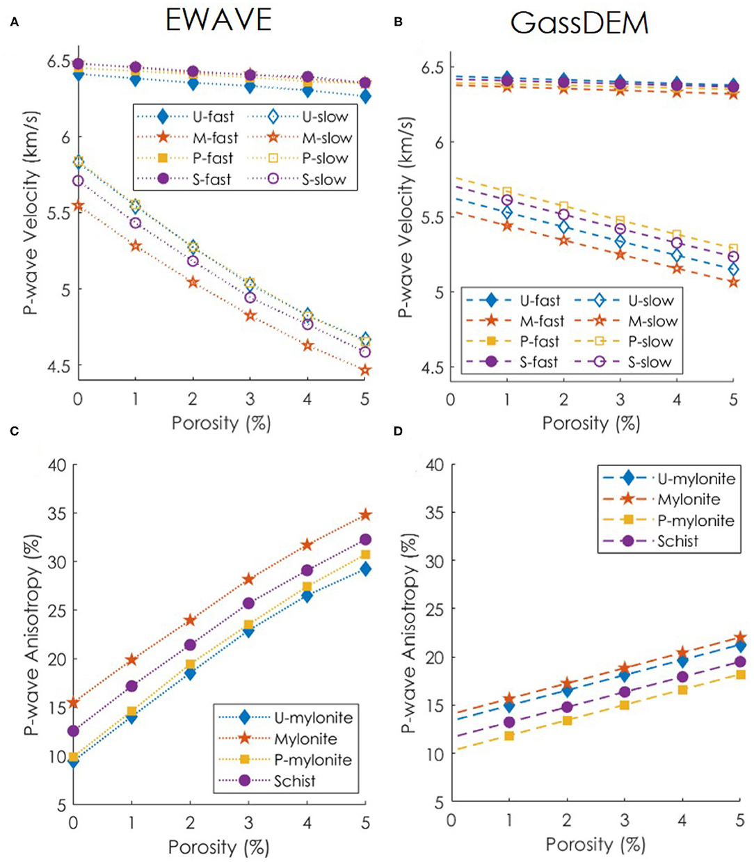
Figure 8. Modeled P-wave velocity and anisotropy with (A,C) EWAVE model (5:1 fracture aspect ratio) and (B,D) GassDEM model (5:2:1 fracture aspect ratio). U, M, P, S refer to ultramylonite, mylonite, protomylonite and schist, respectively. -fast and -slow refer to fast and slow velocity.

3.4. Differential Effective Medium Modeling (MTEX and GassDEM)

The fast and slow velocities estimated with MTEX have similar values to the EWAVE modeling at approximately 6.5 and 5.5–6.0 km/s, respectively. Foliation-parallel ellipsoidal fractures of aspect ratio 5:2:1 are added to the model for porosity volume from 0.1 to 5% at 0.1% increments. The fast velocities decrease from 6.5 to 6.3 km/s at 5% porosity (Figure 8B), while the slow velocities decrease from 5.5 to 5 km/s. The pore-free P-wave anisotropy ranges from 10 to 15% and increases to 15–20% for a 5% porosity. Although EWAVE and GassDEM/MTEX use the same fracture volume and orientation, slow velocities - and thus P-wave anisotropy—greatly differ between the models. The P-wave velocity and anisotropy results for the section cut at 30^o from foliation and water-filled samples are presented in the Supplementary Material.

The previous models assumed that all fractures are the same size and align with foliation. Fractures in real rocks however, vary in size and orient in different directions. For this, we use the modified GassDEM code (Simpson et al., 2020) to model how different combinations of foliation, parallel and randomly oriented fractures, as well as fracture size, affect P-wave velocities. Two fracture aspect ratios are used: a 5:2:1 aspect ratio which used in this study, and a 50:50:1 ratio as a representative of flat fractures. Eleven fracture orientation combinations are modeled from 0% aligned (random) fractures, to 100% aligned fractures, with combinations of these. Because all rocks show similar velocity and anisotropy trends, only the protomylonite data are used in this model. The P-wave velocities and anisotropy of all fracture models are calculated as a function of propagation angle to foliation. At 90^o the P-wave propagates parallel to foliation, and at 180^o perpendicular to it.

For the flat-shaped pore of 5:2:1 aspect ratio (Figure 9A), the fracture alignment can increase and decrease the fast and slow P-wave velocity, respectively, by approximately 0.4 km/s. Velocity changes become more prominent for the flatter aspect ratio fractures (50:50:1) resulting in overall slower velocities for all azimuthal directions compared to fractures of 5:2:1 aspect ratio (Figure 9B). The aligned fractures with a 50:50:1 aspect ratio increase the fast velocity by 3 km/s and decrease the slow velocity by 1.5 km/s. Fracture porosity has more influence on the P-wave anisotropy as more fractures are aligned (Figures 9C,D). However, when fracture alignment drops below 30% the anisotropy decreases with porosity instead.

FIGURE 9

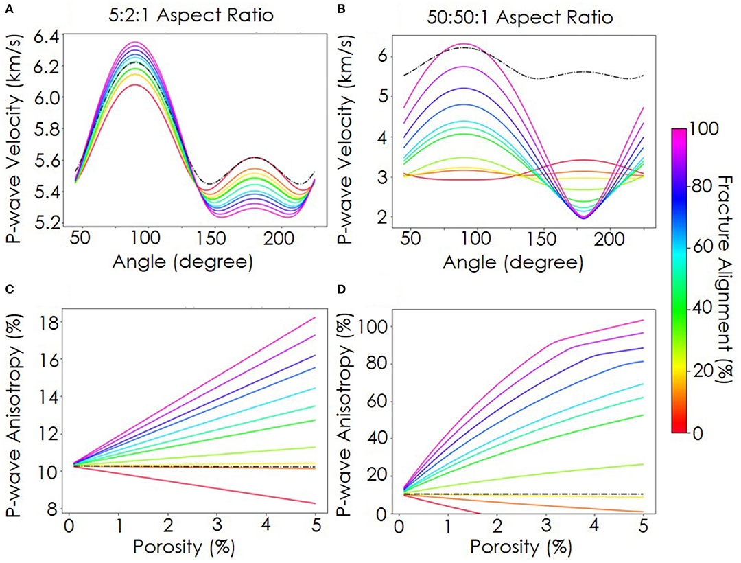
Figure 9. P-wave velocity and anisotropy with angles of propagation to foliation for a 5% porosity protomylonite from GassDEM modeling. Two aspect ratios are compared: (A,C) 5:2:1 and (B,D) 50:50:1. The color represents fracture alignment to foliation, from all fractures being randomly oriented (0%) to perfectly aligned fractures to foliation (100%), and combinations of these. The black dashed lines are results for a rock with 100% spherical pores (1:1:1 aspect ratio) for reference.

The modeled velocity using spherical pores (black dashed lines) is presented for comparison (Figure 9). The spherical pore model yields a similar fast velocity to the model including 30% aligned fractures of 5:2:1 aspect ratio. The slow velocity of the 100% randomly oriented fracture model coincides only with the model that only contains spherical pores. For the 50:50:1 models, the fast velocity from the spherical pore model is comparable to the perfectly aligned 50:50:1 pore aspect ratio model. However, the 50:50:1 pore model's slow velocity is significantly lower than that of the spherical pore model. The anisotropy of the spherical pore model remains almost constant and equal to the pore-free anisotropy because spherical pores reduce P-wave velocity equally, regardless of direction as opposed to fractures. If only 10–20% of the fractures align with foliation, then the P-wave anisotropy is equal to that of a rock with the same porosity but made up of spherical pores. This is observed for fractures of both aspect ratios investigated here.

4. Discussion

4.1. P-Wave Velocity: EWAVE vs. MTEX-DEM

Pore-free rock P-wave velocities and anisotropy were calculated using the wave propagation model (EWAVE) and the Hill average effective medium model (MTEX), for samples cut perpendicular to foliation. The pore-free EWAVE and Hill average MTEX modeled velocities (velocities at 0% porosity in Figure 8A) are consistent between both methods, which is similar to observations by Zhong et al. (2014). As mentioned above, the non-indexed phases by EBSD are assumed to be mica. Based on Toy et al. (2008) and Dempsey et al. (2011), we also assume that most mica basal planes are parallel to foliation (80:20 parallel:random to foliation). Nonetheless, future studies should perform analyses capable of quantifying mica CPO on these mylonites to conclude on the true extent of the influence of mineralogy on the Alpine Fault rock anisotropy.

EWAVE and MTEX-GassDEM models are used to calculate the fractured rock P-wave velocity. A key difference between the model is that the GassDEM models a 3D pore, while the EWAVE model uses either natural rock fractures (e.g., extracted from micro-imaging techniques) or simplified 2D fractures, as done in this study. The simplified 2D fracture shape misses one dimension of the aspect ratio. For example, fractures with a 5:2:1 and 5:5:1 ratio would be simplified to a 5:1 2D ratio.

Individually these two types of 3D fractures (5:2:1 and 5:5:1) result in different GassDEM wave velocities, which also differ even more from the EWAVE modeled velocities using a 5:1 2D pore shape (Figure 10). The effect of pore aspect ratio on the fast velocities is insignificant. However, the 5:1 aspect ratio slow velocity deviates from the 5:2:1 and 5:5:1 aspect ratio trends by 12% and 5.3% at 5% porosity, respectively. As a result, the 5:1 ratio yields almost double the anisotropy of the 5:2:1 ratio.

FIGURE 10

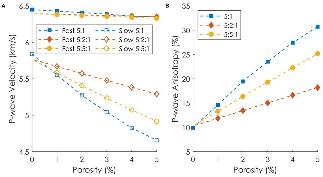
Figure 10. Comparison between (A) modeled P-wave velocities and (B) P-wave anisotropy of the three rock models with three different pore aspect ratios: 5:1 (2D), 5:2:1 (3D), and 5:5:1 (3D).

A discrepancy between the elastic modeling using 2D and 3D data and their relationship has been previously reported (e.g., Saxena and Mavko, 2016; Hooghvorst et al., 2020). Because the 2D EWAVE model assumes a plane wave perpendicular to the EBSD model (Zhong and Frehner, 2018), the pore or fracture length perpendicular to the EBSD 2D model is thus assumed to be infinitely long. This is in contrast with the finite shape of the fracture used in the 3D GassDEM model. In this study, a simplified 2D pore shape is determined by reducing the 3D aspect ratio X:Y:1 to X:1. Having an infinitely long Y-axis in such a way contradicts this pore dimension reduction assumption and such infinite fractures exaggerate the effect of pores on the P-wave velocity. This explains why the modeled slow velocities from the 2D EWAVE model are always lower than those of the 3D GassDEM model. A key conclusion is that both the 2D and 3D pore aspect ratios strongly affect the modeled P-wave velocity and anisotropy. While both EWAVE and GassDEM models provide similar velocity predictions for pore-free rocks, a well-constrained pore shape in 3D is needed to accurately model P-wave velocity and anisotropy in a porous medium.

4.2. Pore Aspect Ratio Assumption

This study makes three assumptions regarding the pore aspect ratio used in EWAVE and GassDEM velocity modeling. First, all pores in a rock are assumed to have the same shape based on the average aspect ratio extracted from the micro-CT data. The average aspect ratio used in our models (5:2:1) is different from that of other works. For example, Vasin et al. (2013) uses a pore aspect ratio of 100:100:1 and 50:50:1 to model shale elasticity. Microfractures in shales also form parallel to layering, in particular, between clay platelets. The pore aspect ratio used in GassDEM modeling is referred to as an effective pore aspect ratio (e.g., Hong-Bing et al., 2013). It is the aspect ratio that best predicts the elasticity from experimental/field measurements at a fixed given porosity. Given that rocks contain various pore shapes and orientations, assuming one aspect ratio is idealistic and would not match all the real pore shapes in a rock.

Figure 4 shows that a pore network is composed of several connected pores of different shapes, sizes and orientations. The pore aspect ratio used in this work (5:2:1) represents the average pore shape of the whole rock, not individual pores which have a wide range of shapes (Figure 6). Finding a representative pore aspect ratio is challenging, but predicting pore shapes and volumes from laboratory data (Adam et al., 2020; Simpson et al., 2020) can be aided by modeling constrained micro-CT analysis for variable shapes and volumes of pores.

Second, we assumed that all lithologies of the shear zone and metamorphic Alpine Fault rocks in this study have the same pore shape. This assumption results in the same velocity relationship with porosity for all lithologies. Figure 6 shows that a similar dominant pore shape is estimated from the micro-CT data for all rocks. However, the pore shape distributions are different, pointing at the fact that the shape of individual pores could be different. In particular, the mylonite has flatness and elongation distributions that slightly differ from the protomylonite and ultramylonite.

Third, while modeling aligned fractures, we assumed that all pores have their longest axis aligned parallel to the rock foliation. Although this is the dominant direction for many microfractures, it is not realistic because not all pores align in the same direction in real rocks. A previous study on serpentinite (Kim et al., 2019) shows that a fracture effect on P-wave velocity is directionally dependent on fracture alignment. In our study, the fracture effect on velocity reduction is minimized when fractures align with wave propagation direction, and maximized when fractures align normal to the propagation direction. This results in the slow velocity being more susceptible to a change on fracture porosity than the fast velocity.

4.3. Velocity Comparison With Previous Studies

The pore-free modeled velocities of this study are compared to previous Alpine Fault EBSD-based velocity modeling works. The fast and slow pore-free velocities from this study (6.4 km/s, 5.5–5.9 km/s) are slightly higher than the velocities (6.2 km/s, 5.5 km/s) reported by Dempsey et al. (2011) but lower than the velocities (6.8–7.0 km/s, 5.7 km/s) reported by Adam et al. (2020). We suspect two possible causes for this discrepancy: mica volume and orientation. The rock samples Dempsey et al. (2011) analyzed contain 15-20 vol.% mica and their mica orientation is extracted from the EBSD data. Adam et al. (2020) worked with samples with a mica content of 35–40 vol.% and the orientation is assumed to align parallel to the rock foliation. In our study however, the samples contain 20–30 vol.% mica and only 80% of micas are assumed to align with foliation. This shows that understanding and quantifying volumes and orientations of mica-dominated rocks are critical to the estimation of seismic wave anisotropy.

We now compare our modeled velocity with the velocity measurements of Alpine Fault rock samples reported in previous studies (Okaya et al., 1995; Allen et al., 2017; Simpson et al., 2019; Adam et al., 2020). The velocities were measured under high confining pressure, thus assumed to be pore-free. The reported experimental fast and slow velocities range between 6.2–6.7 and 5.0–5.7 km/s, respectively. The velocities from this study fall within these ranges. Okaya et al. (1995) reports an increase in P-wave anisotropy toward the Alpine Fault plane. They interpret this increase in anisotropy as a result of increasing mica alignment due to metamorphism. Although we were unable to image mica orientations, we note that a 12% difference in mica volume fraction with 80% of micas being aligned with foliation can result in almost 5% increase in P-wave anisotropy (Figure 8D, Table 2). We further show that even small volumes of microfractures can significantly affect anisotropy. Adam et al. (2020) show that such fractures can remain open at 4 km depths at the Alpine Fault.

Field seismic data show that the rock in the vicinity of the Alpine Fault has a fast velocity of 6.2-6.5 km/s and a slow velocity of 5.6–5.7 km/s (Godfrey et al., 2002; Stern et al., 2007), which agrees with the velocities in this study. Additionally, the fluid-interpreted low velocity zone of 5.5 km/s velocity is also reported (Stern and McBride, 1998; Stern et al., 2007). Our porosity and fracture orientation models (Figure 9) predict the field velocities in the following sense: the fracture aspect ratio is 5:2:1 and 80% of fractures align with foliation while the rest are randomly oriented. It is important to recall that GassDEM models are non-unique, and different combinations of porosity, pore aspect ratio and orientation can result in identical velocity predictions.

5. Conclusion

In this study, P-wave elastic wave speeds in Alpine Fault rocks are modeled with and without microfractures. The four lithologies represent the protolith and the shear zone of the Alpine Fault: schist, protomylonite, mylonite and ultramylonite. Although samples were cut at 30^o and 90^o angles to foliation, the tiny mica minerals were not indexed in the EBSD analysis for both orientations. Through numerical modeling and laboratory data, the orientation of the micas is assumed to be 80% aligned to foliation and 20% random. Because all lithologies have similar mica volumes, the pore-free wave velocities and anisotropies are similar among the samples. However, we were not able to quantify mica CPO because of limitations of EBSD imaging of such small crystals. Therefore, it remains inconclusive whether variable mica CPO between the Alpine Fault lithology can have any significant influence on P-wave anisotropy.

The effect of fractures on the P-wave anisotropy of fault zone mylonite is the most important result of our study. Three sets of micro-CT data of protomylonite, mylonite and ultramylonite are analyzed to quantitatively extract porosity and pore shape information with a resulting average pore aspect ratio of 5:2:1 across all lithologies. Pore-free wave velocities are similarly predicted by EWAVE and MTEX. However, significant differences arise in the slow P-wave velocity prediction (i.e., anisotropy) when fractures are included as 2D rectangles (EWAVE) or 3D ellipsoids (GassDEM). The type of method used to model fractures can double the P-wave anisotropy in these rocks for a constant porosity. It is thus critical to understand how each numerical model approaches microfractures and to constrain shapes and volumes of such fractures with quantitative microstructural analysis.

Data Availability Statement

The original contributions presented in the study are included in the article/Supplementary Material, further inquiries can be directed to the corresponding author/s.

Author Contributions

JC prepared the thin sections, acquired EBSD data and performed the numerical models for this manuscript. LA developed the idea, co-wrote the manuscript and advised JC. VT and MO helped with the design and acquisition of the EBDS data and thin section preparation and revised the manuscript. BS and VT provided the micro-CT data. JS provided a modified GassDEM code and helped via discussions on numerical modeling. XZ provided advice on the EWAVE code and ways to modify it to include fractures.

Funding

We thank the Royal Society of New Zealand, Marsden Contract #14-UOA-028. The Avizo software and workstation employed were supported by Nvidia Corporation who donated the Titan X Pascal GPU, the Royal Society of New Zealand Rutherford Discovery Fellowship (RDF) 16-UOO-1602 and a subcontract to GNS Science (GNS-MBIE00056). Synchrotron and electron microscopic data acquisition was supported by RDF 16-UOO-1602, and SPring8 Proposals No. 2017B1378 and 2018A1506.

Conflict of Interest

The authors declare that the research was conducted in the absence of any commercial or financial relationships that could be construed as a potential conflict of interest.

Acknowledgments

We would like to thank Marianne Negrini for helping with the EBSD experiments. We also thank Andres Arcila-Rivera and Brent Pooley for helping with the sample preparation. Analyzing of the micro-CT data was assisted by Francesco Cappuccio.

Supplementary Material

The Supplementary Material for this article can be found online at: https://www.frontiersin.org/articles/10.3389/feart.2021.645532/full#supplementary-material

References

Adam, L., Frehner, M., Sauer, K., Toy, V., and Guerin-Marthe, S. (2020). Seismic anisotropy and its impact on imaging the Alpine Fault: an experimental and modeling perspective. J. Geophys. Res. 125:e2019JB019029. doi: 10.1029/2019JB019029

CrossRef Full Text | Google Scholar

Alexandrov, K. S., and Ryzhova, T. V. (1961). Elastic properties of rock-forming minerals. II. Layered silicates. Izv. Acad. Sci. USSR Geophys.Ser. 12, 165–1168.

Google Scholar

Allen, M. J., Tatham, D., Faulkner, D. R., Mariani, E., and Boulton, C. (2017). Permeability and seismic velocity and their anisotropy across the Alpine Fault, New Zealand: an insight from laboratory measurements on core from the Deep Fault Drilling Project phase 1 (DFDP-1). J. Geophys. Res. Solid Earth 122, 6160–6179. doi: 10.1002/2017JB014355

CrossRef Full Text | Google Scholar

Bass, J. D. (1995). Elasticity of minerals, glasses, and melts. Miner. Phys. Crystallogr. 23, 45–63. doi: 10.1029/RF002p0045

CrossRef Full Text | Google Scholar

Boulton, C., Menzies, C. D., Toy, V. G., Townend, J., and Sutherland, R. (2017). Geochemical and microstructural evidence for interseismic changes in fault zone permeability and strength, Alpine Fault, New Zealand. Geochem. Geophys. Geosyst. 18, 238–265. doi: 10.1002/2016GC006588

CrossRef Full Text | Google Scholar

Brown, J. M., Angel, R. J., and Ross, N. L. (2016). Elasticity of plagioclase feldspars. J. Geophys. Res. Solid Earth 121, 663–675. doi: 10.1002/2015JB012736

CrossRef Full Text | Google Scholar

Bruggeman, D. (1935). Berechnung verschiedener konstanten von heterogenen substanzen: 1. dielektrizitatskonstanten und leitfahigkeiten der mischkorper aus isotropen substanzen. Ann. Phys. 24, 636–679. doi: 10.1002/andp.19354160705

CrossRef Full Text

Chapman, C. H., and Pratt, R. G. (1992). Traveltime tomography in anisotropic media—I. Theory. Geophys. J. Int. 109, 1–19. doi: 10.1111/j.1365-246X.1992.tb00075.x

CrossRef Full Text | Google Scholar

Chen, G., Cooke, J. A., Gwanmesia, G. D., and Liebermann, R. C. (1999). Elastic wave velocities of Mg₃Al₂2Si₃O₁2-pyrope garnet to 10 GPa. Am. Mineral. 84, 384–388. doi: 10.2138/am-1999-0322

CrossRef Full Text | Google Scholar

Christensen, N., and Okaya, D. (2007). Compressional and Shear Wave Velocities in South Island, New Zealand Rocks and Their Application to the Interpretation of Seismological Models of the New Zealand Crust. Washington, DC: American Geophysical Union Geophysical Monograph Series, 123–155.

Google Scholar

Columbus, J., Sirguey, P., and Tenzer, R. (2011). A free, fully assessed 15-m dem for New Zealand. Surv. Q. 66, 16–19.

Google Scholar

Cooper, A., and Palin, J. (2018). Two-sided accretion and polyphase metamorphism in the Haast Schist belt, New Zealand: constraints from detrital zircon geochronology. GSA Bull. 130, 1501–1518. doi: 10.1130/B31826.1

CrossRef Full Text | Google Scholar

Dempsey, E. D., Prior, D. J., Mariani, E., Toy, V. G., and Tatham, D. J. (2011). Mica-controlled anisotropy within mid-to-upper crustal mylonites: an EBSD study of mica fabrics in the Alpine Fault Zone, New Zealand. Geol. Soc. Lond. Spec. Publ. 360, 33–47. doi: 10.1144/SP360.3

CrossRef Full Text | Google Scholar

Eccles, J. D., Gulley, A. K., Malin, P. E., Boese, C. M., Townend, J., and Sutherland, R. (2015). Fault zone guided wave generation on the locked, late interseismic Alpine Fault, New Zealand. Geophys. Res. Lett. 42, 5736–5743. doi: 10.1002/2015GL064208

CrossRef Full Text | Google Scholar

Edbrooke, S. W., Heron, D. W., Forsyth, P. J., and Jongens, R. (2015). Geological map of New Zealand 1: 1,000,000, GNS Science Geological Map 2, 2 print maps. Lower Hut: GNS Science."

Feenstra, J., Thurber, C., Townend, J., Roecker, S., Bannister, S., Boese, C., et al. (2016). Microseismicity and P-wave tomography of the central Alpine Fault, New Zealand. N. Z. J. Geol. Geophys. 59, 483–495. doi: 10.1080/00288306.2016.1182561

CrossRef Full Text | Google Scholar

Gassmann, F. (1951). Uber die elastizitat poroser medien. Vierteljahrssch. Naturforsch. Gesellsch. Zurich 96, 1–23.

Google Scholar

Godfrey, N. J., Christensen, N. I., and Okaya, D. A. (2000). Anisotropy of schists: contribution of crustal anisotropy to active source seismic experiments and shear wave splitting observations. J. Geophys. Res. Solid Earth 105, 27991–28007. doi: 10.1029/2000JB900286

CrossRef Full Text | Google Scholar

Godfrey, N. J., Christensen, N. I., and Okaya, D. A. (2002). The effect of crustal anisotropy on reflector depth and velocity determination from wide-angle seismic data: a synthetic example based on South Island, New Zealand. Tectonophysics 355, 145–161. doi: 10.1016/S0040-1951(02)00138-5

CrossRef Full Text | Google Scholar

Grapes, R., and Watanabe, T. (1994). Mineral composition variation in Alpine Schist, Southern Alps, New Zealand: implications for recrystallization and exhumation. Island Arc 3, 163–181.

Google Scholar

Heyliger, P., Ledbetter, H., and Kim, S. (2003). Elastic constants of natural quartz. J. Acoust. Soc. Am. 114, 644–650. doi: 10.1121/1.1593063

CrossRef Full Text | Google Scholar

Hong-Bing, L., Jia-Jia, Z., and Feng-Chang, Y. (2013). Inversion of effective pore aspect ratios for porous rocks and its applications. Chinese J. Geophys. 56, 43–51. doi: 10.1002/cjg2.20004

CrossRef Full Text | Google Scholar

Hooghvorst, J. J., Harrold, T. W. D., Nikolinakou, M. A., Fernandez, O., and Marcuello, A. (2020). Comparison of stresses in 3D vs. 2D geomechanical modelling of salt structures in the Tarfaya Basin, West African coast. Petrol. Geosci. 26, 36–49. doi: 10.1144/petgeo2018-095

CrossRef Full Text | Google Scholar

Howarth, J. D., Cochran, U. A., Langridge, R. M., Clark, K., Fitzsimons, S. J., Berryman, K., et al. (2018). Past large earthquakes on the Alpine Fault: paleoseismological progress and future directions. N. Z. J. Geol. Geophys. 61, 309–328. doi: 10.1080/00288306.2018.1464658

CrossRef Full Text | Google Scholar

Jeppson, T. N., and Tobin, H. J. (2020). Elastic properties and seismic anisotropy across the Alpine Fault, new zealand. Geochem. Geophys. Geosyst. 21:e2020GC009073. doi: 10.1029/2020GC009073

CrossRef Full Text | Google Scholar

Karalliyadda, S. C., and Savage, M. K. (2013). Seismic anisotropy and lithospheric deformation of the plate-boundary zone in South Island, New Zealand: inferences from local S-wave splitting. Geophys. J. Int. 193, 507–530. doi: 10.1093/gji/ggt022

CrossRef Full Text | Google Scholar

Kelly, C. M., Faulkner, D. R., and Rietbrock, A. (2017). Seismically invisible fault zones : laboratory insights into imaging faults in anisotropic rocks. Geophys. Res. Lett. 44, 8205–8212. doi: 10.1002/2017GL073726

CrossRef Full Text | Google Scholar

Kern, H., Ivankina, T. I., Nikitin, A. N., Lokajíček, T., and Pros, Z. (2008). The effect of oriented microcracks and crystallographic and shape preferred orientation on bulk elastic anisotropy of a foliated biotite gneiss from Outokumpu. Tectonophysics 457, 143–149. doi: 10.1016/j.tecto.2008.06.015

CrossRef Full Text | Google Scholar

Kim, Y., Kim, E., and Mainprice, D. (2019). GassDem: a MATLAB program for modeling the anisotropic seismic properties of porous medium using differential effective medium theory and Gassmann's poroelastic relationship. Comput. Geosci. 126, 131–141. doi: 10.1016/j.cageo.2019.02.008

CrossRef Full Text | Google Scholar

Lay, V., Buske, S., Lukács, A., Gorman, A. R., Bannister, S., and Schmitt, D. R. (2016). Advanced seismic imaging techniques characterize the Alpine Fault at Whataroa (New Zealand). J. Geophys. Res. Solid Earth 121, 8792–8812. doi: 10.1002/2016JB013534

CrossRef Full Text | Google Scholar

Little, T. A., Holcombe, R. J., and Ilg, B. R. (2002). Kinematics of oblique collision and ramping inferred from microstructures and strain in middle crustal rocks, central Southern Alps, New Zealand. J. Struct. Geol. 24, 219–239. doi: 10.1016/S0191-8141(01)00060-8

CrossRef Full Text | Google Scholar

Loucks, R. G., Reed, R. M., Ruppel, S. C., and Jarvie, D. M. (2009). Morphology, genesis, and distribution of nanometer-scale pores in siliceous mudstones of the Mississippian Barnett Shale. J. Sediment. Res. 79, 848–861. doi: 10.2110/jsr.2009.092

CrossRef Full Text | Google Scholar

Mainprice, D., Bachmann, F., Hielscher, R., Schaeben, H., and Lloyd, G. E. (2015). Calculating anisotropic piezoelectric properties from texture data using the MTEX open source package. Geol. Soc. Lond. Spec. Publ. 409, 223–249. doi: 10.1144/SP409.2

CrossRef Full Text | Google Scholar

Naus-Thijssen, F. M. J., Johnson, S. E., and Koons, P. O. (2010). Numerical modeling of crenulation cleavage development: a polymineralic approach. J. Struct. Geol. 32, 330–341. doi: 10.1016/j.jsg.2010.01.004

CrossRef Full Text | Google Scholar

Norris, R. J., and Cooper, A. F. (1997). Erosional control on the structural evolution of a transpressional thrust complex on the Alpine fault, New Zealand. J. Struct. Geol. 19, 1323–1342. doi: 10.1016/S0191-8141(97)00036-9

CrossRef Full Text | Google Scholar

Norris, R. J., and Cooper, A. F. (2007). The Alpine Fault, New Zealand: Surface Geology and Field Relationships. American Geophysical Union (AGU), 157–175.

Google Scholar

Novitsky, C. G., Holbrook, W. S., Carr, B. J., Pasquet, S., Okaya, D., and Flinchum, B. A. (2018). Mapping inherited fractures in the critical zone using seismic anisotropy from circular surveys. Geophys. Res. Lett. 45, 3126–3135. doi: 10.1002/2017GL075976

CrossRef Full Text | Google Scholar

Okaya, D., Christensen, N., Stanley, D., Stern, T., and Group, S. I. G. T. S. W. (1995). Crustal anisotropy in the vicinity of the Alpine Fault Zone, South Island, New Zealand. N. Z. J. Geol. Geophys. 38, 579–583.

Google Scholar

Pischiutta, M., Savage, M. K., Holt, R. A., and Salvini, F. (2015). Fracture-related wavefield polarization and seismic anisotropy across the Greendale Fault. J. Geophys. Res. Solid Earth 120, 7048–7067. doi: 10.1002/2014JB011560

CrossRef Full Text | Google Scholar

Prior, D., and Mariani, E. (2009). EBSD in the Earth Sciences: Applications, Common Practice, and Challenges. Electron Backscatter Diffraction in Materials ScienceElectron Backscatter Diffraction in Materials Science. Boston, MA: Springer, 345–360.

Google Scholar

Savage, M. K., Duclos, M., and Marson-Pidgeon, K. (2007). Seismic Anisotropy in South Island, New Zealand. A Continental Plate Boundary: Tectonics at South Island, New Zealand. Washington, DC: American Geophysical Union, 95–114.

Google Scholar

Saxena, N., and Mavko, G. (2016). Estimating elastic moduli of rocks from thin sections: digital rock study of 3D properties from 2D images. Comput. Geosci. 88, 9–21. doi: 10.1016/j.cageo.2015.12.008

CrossRef Full Text | Google Scholar

Schuck, B., Schleicher, A. M., Janssen, C., Toy, V. G., and Dresen, G. (2020). Fault zone architecture of a large plate-bounding strike-slip fault: a case study from the Alpine Fault, New Zealand. Solid Earth 11, 95–124. doi: 10.5194/se-11-95-2020

CrossRef Full Text | Google Scholar

Simpson, J., Adam, L., van Wijk, K., and Charoensawan, J. (2020). Constraining microfractures in foliated Alpine Fault rocks with laser ultrasonics. Geophys. Res. Lett. 47:e2020GL087378. doi: 10.1029/2020GL087378

CrossRef Full Text | Google Scholar

Simpson, J., van Wijk, K., Adam, L., and Smith, C. (2019). Laser ultrasonic measurements to estimate the elastic properties of rock samples under in situ conditions. Rev. Sci. Instrum. 90:114503. doi: 10.1063/1.5120078

PubMed Abstract | CrossRef Full Text | Google Scholar

Smith, E. G. C., Stern, T., and O'Brien, B. (1995). A seismic velocity profile across the central South Island, New Zealand, from explosion data. N. Z. J. Geol. Geophys. 38, 565–570. doi: 10.1080/00288306.1995.9514684

CrossRef Full Text | Google Scholar

Smith, T. M., Sondergeld, C. H., and Rai, C. S. (2003). Gassmann fluid substitutions: a tutorial. Geophysics 68, 430–440. doi: 10.1190/1.1567211

CrossRef Full Text | Google Scholar

Stern, T., Kleffmann, S., Okaya, D., Scherwath, M., and Bannister, S. (2001). Low seismic-wave speeds and enhanced fluid pressure beneath the Southern Alps of New Zealand. Geology 29, 679–682. doi: 10.1130/0091-7613(2001)029<0679:LSWSAE>2.0.CO;2

CrossRef Full Text | Google Scholar

Stern, T., Okaya, D., Kleffmann, S., Scherwath, M., Henrys, S., and Davey, F. (2007). Geophysical Exploration and Dynamics of the Alpine Fault Zone. A Continental Plate Boundary: Tectonics at South Island, New Zealand. Washington, DC: American Geophysical Union, 207–233.

Google Scholar

Stern, T. A., and McBride, J. H. (1998). Seismic exploration of continental strike-slip zones. Tectonophysics 286, 63–78.

Google Scholar

Sutherland, R., Eberhart-Phillips, D., Harris, R. A., Stern, T., Beavan, J., Ellis, S., et al. (2007). Do Great Earthquakes Occur on the Alpine Fault in Central South Island, New Zealand? A Continental Plate Boundary: Tectonics at South Island, New Zealand. Washington, DC: American Geophysical Union, 235–251.

Toy, V. G., Boulton, C. J., Sutherland, R., Townend, J., Norris, R. J., Little, T. A., et al. (2015). Fault rock lithologies and architecture of the central Alpine fault, New Zealand, revealed by DFDP-1 drilling. Lithosphere 7, 155–173. doi: 10.1130/L395.1

CrossRef Full Text | Google Scholar

Toy, V. G., Prior, D. J., and Norris, R. J. (2008). Quartz fabrics in the Alpine Fault mylonites: Influence of pre-existing preferred orientations on fabric development during progressive uplift. J. Struct. Geol. 30, 602–621. doi: 10.1016/j.jsg.2008.01.001

CrossRef Full Text | Google Scholar

Tsvankin, I., Gaiser, J., Grechka, V., Van Der Baan, M., and Thomsen, L. (2010). Seismic anisotropy in exploration and reservoir characterization: an overview. Geophysics 75, 75A15–75A29. doi: 10.1190/1.3481775

CrossRef Full Text | Google Scholar

Vasin, R. N., Wenk, H., Kanitpanyacharoen, W., Matthies, S., and Wirth, R. (2013). Elastic anisotropy modeling of Kimmeridge shale. J. Geophys. Res. Solid Earth 118, 3931–3956. doi: 10.1002/jgrb.50259

CrossRef Full Text | Google Scholar

Zhong, X., and Frehner, M. (2018). E-Wave software: EBSD-based dynamic wave propagation model for studying seismic anisotropy. Comput. Geosci. 118, 100–108. doi: 10.1016/j.cageo.2018.05.015

CrossRef Full Text | Google Scholar

Zhong, X., Frehner, M., Kunze, K., and Zappone, A. (2014). A novel EBSD-based finite-element wave propagation model for investigating seismic anisotropy: application to Finero peridotite, ivrea-verbano zone, Northern Italy. Geophys. Res. Lett 41, 7105–7114. doi: 10.1002/2014GL060490

CrossRef Full Text | Google Scholar