 James J. Holmes
 Hector Perea
 Neal W. Driscoll1
 Graham M. Kent
- 1Scripps Institution of Oceanography, University of California, San Diego, La Jolla, CA, United States
- 2Faculty of Geological Sciences, Complutense University of Madrid, Madrid, Spain
- 3Nevada Seismological Laboratory, University of Nevada, Reno, Reno, NV, United States
Deformation observed along the San Mateo (SMT) and San Onofre trends (SOT) in southern California has been explained by two opposing structural models, which have very different hazard implications for the coastal region. One model predicts that the deformation is transpressional in a predominantly right lateral fault system with left lateral step-overs. Conversely in the alternative model, the deformation is predicted to be compressional associated with a regional blind thrust that reactivated detachment faults along the continental margin. State-of-the-art 3D P-Cable seismic data were acquired to characterize the geometry and linkage of faults in the SMT and SOT. The new observations provide evidence that deformation along the slope is more consistent with step-over geometry than a regional blind thrust model. For example, regions in the SOT exhibit small scale compressional structures that deflect canyons along jogs in the fault segments across the slope. The deformation observed in the SMT along northwesterly trending faults has a mounded, bulbous character in the swath bathymetry data with steep slopes ( ∼ 25°) separating the toe of the slope and the basin floor. The faulting and folding in the SMT are very localized and occur where the faults trend more northwesterly (average trend ∼ 285°) with the deformation dying away both towards the north and east. In comparison, the SOT faults trend more northerly (average trend ∼ 345°). The boundary between these fault systems is abrupt and characterized by shorter faults that appear to be recording right lateral displacement and possibly accommodating the deformation between the two larger fault systems. Onlapping undeformed turbidite layers reveal that the deformation associated with both major fault systems may be inactive and radiocarbon dating suggests deformation ceased in the middle to late Pleistocene (between 184 and 368 kyr). In summary, our preferred conceptual model for tectonic deformation along the SMT and SOT is best explained by left lateral step-overs along the predominantly right lateral strike-slip fault systems.
Introduction
Southern California’s complex tectonic evolution is recorded by the structural and stratigraphic deformation of the Inner California Borderland (ICB). From the late Oligocene/early Miocene, the cessation of Farallon plate subduction ushered in a tectonic sequence of block rotation and extension (Luyendyk et al., 1985; Scott Hornafius et al., 1986; Lonsdale, 1991; Crouch and Suppe, 1993; Nicholson et al., 1994; Bohannon and Parsons, 1995; Atwater and Stock, 1998). Since the late Miocene to early Pliocene the margin has been overprinted by right-lateral strike-slip motion, often along reactivated Mesozoic structures (Grant and Shearer, 2004; Hill, 1971). Geodetic data (UNAVCO Community, 2005) shows a northwestward trend in movement relative to interior North America (cyan arrows in Figure 1). The majority of the slip budget between North America and Pacific plates is accommodated by onshore faulting (primarily east of the Elsinore fault systems, EF; Figure 1); however, approximately 5–8 mm/yr, or nearly 15% of relative plate motion, is partitioned offshore between a network of northwest-trending strike-slip fault systems ranging from just east of San Clemente Island to the coastline (Bennett et al., 1996; Ryan et al., 2012; Sahakian et al., 2017).
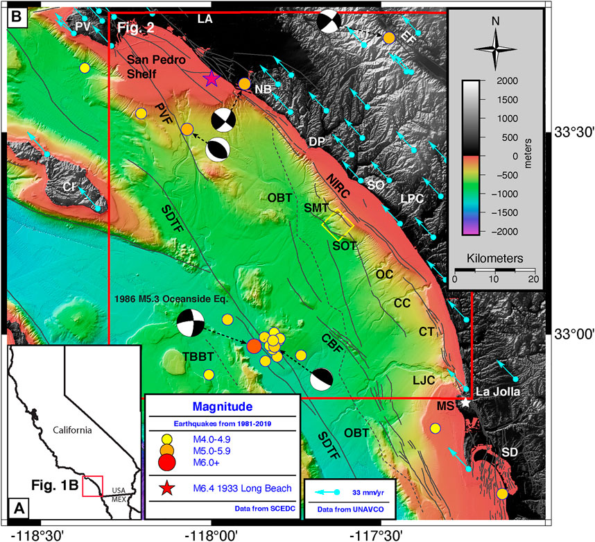
FIGURE 1. (A) Regional map of California State showing the location of Panel 1B (red box). (B) Area map of Inner California Borderland relative to the southern California coast. Red box outlines the area shown in Figure 2. Yellow rectangle outlines the survey area. Solid and dashed gray faults are from USGS Fault and Fold database (U.S. Geological Survey, 2006). Dashed faults denote the possible Oceanside blind thrust (OBT) and Thirtymile Bank blind thrust (TBBT). Colored dots represent epicenters of earthquakes with magnitudes 4+ between 1981 and 2019 (SCEDC, 2013). Focal mechanisms are downloaded from SCEDC for earthquakes from 1981 to 2019. Red star shows epicenter of M6.4 1933 Long Beach earthquake. White star shows location of Mount Soledad. Bathymetry from Dartnell et al. (2015). Cyan arrows show GPS plate velocity vectors with respect to a fixed interior North America reference frame (NAM14) (data from UNAVCO). Abbreviations: CBF, Coronado Bank Fault; CC, Carlsbad Canyon; CI, Catalina Island; CT, Carlsbad Trend; DP, Dana Point; LA, Los Angeles; LJC, La Jolla Canyon; LPC, Las Pulgas Canyon; MS, Mount Soledad; NIRC, Newport-Inglewood Rose Canyon Fault; NB, Newport Beach; OBT, Oceanside blind thrusts; OC, Oceanside Canyon; PV, Palos Verdes; PVF, Palos Verdes Fault; SCI, San Clemente Island; SD, San Diego; SDTF, San Diego Trough Fault; SMT, San Mateo Trend; SO, San Onofre State Beach; SOT, San Onofre Trend; TBBT, Thirtymile Bank blind thrust.
Legg and Kennedy (1979) divided the major strike-slip fault systems of the ICB into four distinct subparallel groups (from west to east): the Santa Cruz-San Clemente, the San Pedro-San Diego Trough, the Palos Verdes Hills-Coronado Banks and the Newport-Inglewood Rose Canyon fault zone. The Newport-Inglewood Rose Canyon system is located predominantly offshore of the southern California margin (Figure 1, labeled “NIRC”). The Newport-Inglewood Rose Canyon system is a steeply dipping right-lateral strike-slip system nearly 120 km long and is composed of several discontinuous splays and trends, characteristic of wrench faulting (Moody and Hill, 1956). The system runs onshore from downtown San Diego to La Jolla, then strikes roughly northwestward about 8–10 km off the coast until reemerging onshore at the San Joaquin Hills near the community of Newport Beach (Sahakian et al., 2017) (Figure 1, labeled “NB”). Paleoseismological work published by Lindvall and Rockwell (1995) reveals a Holocene slip rate of 1.5–2.0 mm/yr on the southern onshore segment. The slip rate for the northern onshore segment is 0.35–0.55 mm/yr based on cone penetration tests (Grant et al., 1997) and well data (Freeman et al., 1992).
Near-shore ICB fault systems are in close proximity to the California cities of Los Angeles, Orange, San Diego, and Tijuana, Mexico. With a combined population greater than 15 million people (Wilson and Fischetti, 2010), these communities together constitute some of the most densely populated coastline in North America. In recent years, high-resolution seismic data acquisition targeting specific fault systems has added considerable information to models of fault segmentation and kinematic constraints in the region (Ryan et al., 2012; Brothers et al., 2015; Sahakian et al., 2017; Conrad et al., 2018), but there are still fault systems in the ICB region that remain poorly characterized today, including systems located near populated areas.
Between Dana Point and Las Pulgas canyon (DP and LPC in Figures 1, 2), there are two fault trends approximately parallel to the Newport-Inglewood Rose Canyon fault system, the San Onofre (SOT) and San Mateo (SMT) trends (Figures 1, 2). It is important to note, the GPS plate velocity vectors have a more northerly trend then these two systems (Figure 1). Some studies propose that the systems are related to regional compression along low angle thrusts (Rivero et al., 2000; Rivero and Shaw, 2011); other works suggest that those systems are dominated by transpression along steeply dipping strike slip faults (Maloney et al., 2016). We conducted a high-resolution 3D multichannel seismic (MCS) survey of the San Onofre and San Mateo trends offshore southern California with the objective of revealing the fault system geometry and fault interaction on this complex structural system to test between the two alternative hypotheses.
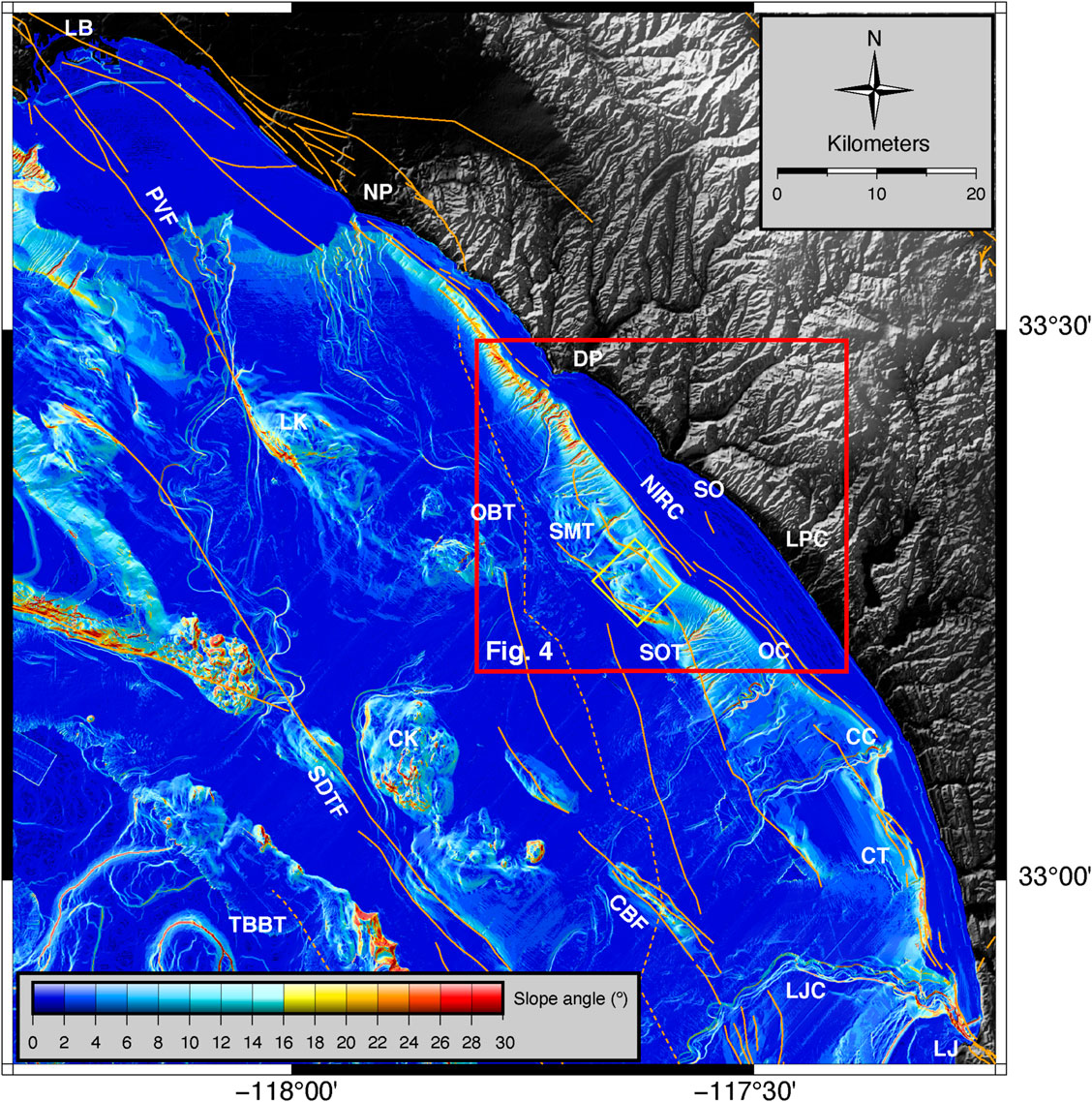
FIGURE 2. Slope map of the offshore southern Inner California Borderland. Warmer colors denote steeper slopes. Solid and dashed orange faults are from USGS Fault and Fold database (U.S. Geological Survey, 2006). Dashed faults denote the possible Oceanside blind thrust (OBT) and Thirtymile Bank blind thrust (TBBT). Red box outlines the area shown in Figure 4. See area location in Figure 1. Abbreviations: DP, Dana Point; LB, Long Beach; LJ, La Jolla; LPC, Las Pulgas Canyon; NP, Newport; SO, San Onofre State Beach.
Methods
3D Seismic Reflection Acquisition and Processing
3D multichannel seismic reflection (MCS) has been the main method of data acquisition of the oil and gas industry for several decades. The main advantage of the 3D data is that it permits a more complete visualization of fault geometry and fault interaction, as well as continuity of subsurface structures and sedimentary units. Recent technological advances allow for the development of portable state-of-the-art 3D MCS systems that can be deployed from ocean-class research vessels (Ebuna et al., 2013; Eriksen et al., 2015). These systems promise high-resolution data at lower costs than standard 3D MCS deployments (Planke et al., 2009a; Planke et al., 2009b).
One such portable high-resolution system, the P-Cable system developed by Geometrics, Inc. employs 14 short (50 m) streamers attached to a cross-cable (Figure 3) (Crutchley and Kopp, 2018). The cross-cable is kept under tension by two one-ton paravanes attached to the ends of the cross-cable on both the port and starboard side of the stern via tow cables. Attached to the cross-cable are the solid-core digital streamers, each containing eight hydrophones. At the head and end of each streamer are digital compasses with depth sensors. The target data horizontal resolution, based on bin size and fold, was 6.25 m. This was dictated by spacing between streamers and between hydrophones in each streamer (Ebuna et al., 2013).
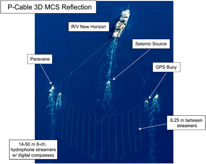
FIGURE 3. Aerial photo of Scripps Institution of Oceanography’s Research Vessel New Horizon towing the P-Cable 3D MCS array during NH1323 cruise in the eastern Gulf of Catalina, with major components of system labeled.
The use of short streamers in the P-Cable array allows for greater operational maneuverability during acquisition and reduces operation concerns, such as time spent in deployment and recovery. In post-processing, short streamers result in reduced aliasing artifacts and higher resolution due to smaller crossline spacing (Brookshire et al., 2016). Shorter streamers are insufficient for extracting rock acoustic velocities via processes such as seismic inversion (Ebuna et al., 2013).
Although we did not depth migrate our 3D volumes due to the lack of velocity data, we adopted the following velocity function described by Ryan et al. (2009) to calculate depth estimations:
Where V represents interval velocities in meters per second, and t is the two-way subsurface travel time (TWTT) in milliseconds. Interval velocities used to derive this function were measured from 2D MCS profiles during Jebco cruise J188SC (Mineral Management Service (MMS), 1997; Triezenberg et al., 2016). This velocity model used to convert travel time to depth was calculated using interval velocities from migrated MCS lines collected in our survey area.
Survey array geometry was tracked by using a set of GPS transmitters positioned at several points on the system: on the paravanes, on the ends of the cross cable, on the seismic source, and on the vessel itself. Tracked changes in system geometry were then corrected during processing.
Our focus was to investigate the different fault systems offshore the San Onofre margin (Figures 2, 4, 5). Prior to the 3D survey, we collected 2D seismic reflection data along the continental shelf and slope aboard the R/V New Horizon (survey NH1320 in 2013). These 2D data were processed and analyzed to select candidate locations for the first high-resolution 3D P-Cable data set (Figures 1, 2, 4, 5). The P-Cable array was towed from the stern of R/V New Horizon (survey NH1323 in 2013; Figure 3).
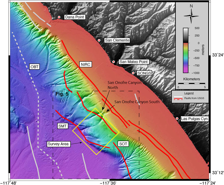
FIGURE 4. Bathymetric map of survey area off San Onofre. 3D seismic survey area bounds on slope is labeled and outlined with yellow rectangles. Red lines show segments of the Newport-Inglewood Rose Canyon (NIRC) fault system, San Mateo trend fault system (SMT), and San Onofre trend fault system (SOT). Light gray lines and dashed lines identify other faults in the area. All fault segments are from USGS Fault and Fold database (U.S. Geological Survey, 2006). Bathymetry from Dartnell et al. (2015). Black dashed line outlines area shown in Figure 5. Red circle with yellow outline denotes location of H4 core described in Covault et al. (2010). Location with respect to Inner California Borderland is shown in Figure 2. Abbreviations: OBT, Oceanside blind thrust; SONGS, San Onofre Nuclear Generation Station.
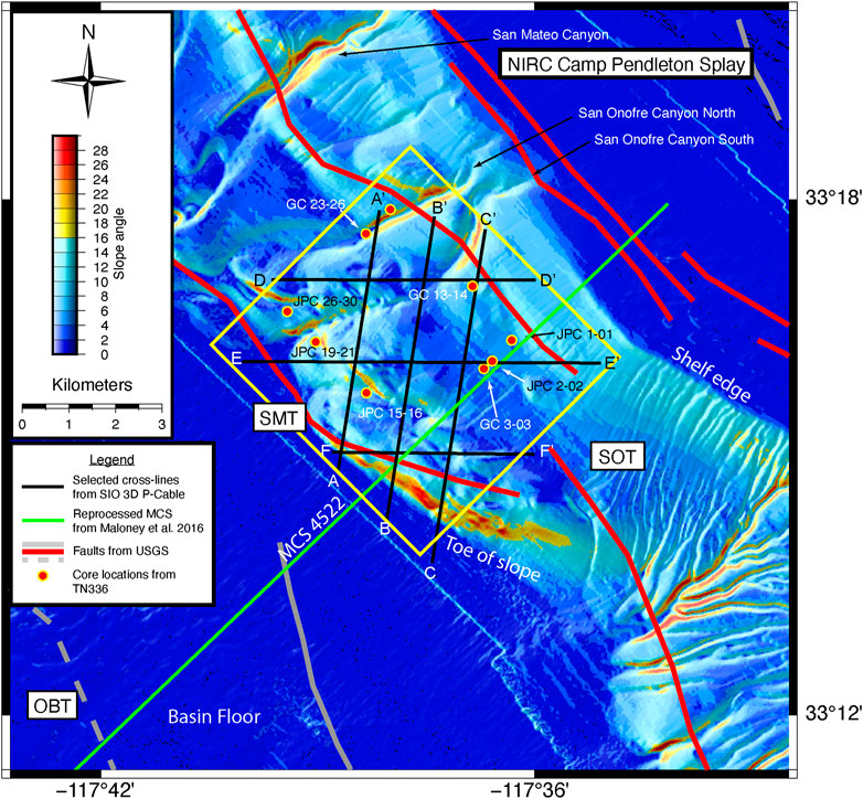
FIGURE 5. Slope map of survey area off San Onofre showing local offshore submarine canyons, and geomorphic features. Red solid lines represent segments of Newport-Inglewood Rose Canyon (NIRC), San Mateo trend (SMT), and San Onofre trend (SOT) fault systems. Solid and dashed gray lines are other faults in the area. All fault segments are from USGS Fault and Fold database (U.S. Geological Survey, 2006). 3D seismic survey is outlined with a yellow rectangle. Green solid line shows location of MCS 4522 (MCS 4522 profile is shown in Figure 11). Blue solid lines denote locations of the seismic arbitrary lines shown in Figures 8 and 9. Red circles with yellow bound show the sampled core locations from the TN336 cruise. Cores prefixed “GC” are gravity cores and “JPC” are jumbo piston cores. See area location in Figure 4. Abbreviation: OBT, Oceanside blind thrust.
We employed a sparker source to acquire data over a 39 km2 square grid, targeted to maximize imaging over the continental slope (Figures 1, 2, 4). Water depths ranged from 182 m to nearly 800 m in depth. Shot intervals constrained a bin size of 6.25 m. A 2,000 ms record length was digitized for the data volume, but much of the data analysis was performed between 0 and 1,600 ms TWTT, where data resolution and imaging were optimum. We measured a peak frequency of 125 Hz that allowed a minimum vertical resolution of 3 m. Shallow structure and deformation were overprinted and masked by the strong reflectors inherent in the seismic source signature.
The 3D data were processed by Geotrace Technologies, a petroleum services company, given the enormous size of the data volume (20 GB per seismic attribute volume) and their previous experience with processing 3D P-Cable data acquired in other surveys (Crutchley and Kopp, 2018). A detailed report outlining the seismic processing workflow is provided in Supplemental Material.
Processed data were compiled into amplitude and similarity-attribute volumes for interpretation. Amplitude volumes image reflectors based on the relative impedance contrast in a trace, while similarity attribute assigns a decimal value to a bin based on the correlation between waveform and amplitude of two or more different nearby traces (Bahorich and Farmer, 1995). In similarity data, a correlative value of 1 represents the state of “perfectly similar”, while a value of 0 represents the state of “completely dissimilar”. While amplitude volumes are useful for imaging and mapping stratigraphic offset within a vertical section, a similarity attribute dataset is valuable for imaging large-scale discontinuities, such as sharply dipping beds, faults, and paleochannels in an isochron (“time-slice”) view.
Additionally, a parameterized dip-steered median filter was applied to the amplitude volume using OpendTect Seismic Interpretation Suite, and following a workflow described by Kluesner and Brothers (2016). This filter increased reflector continuity and facilitated data interpretation (Supplementary Figure S1), which in turn, increased confidence in our interpretations.
We followed an iterative process for interpretation. Initial interpretations were performed on every 20–50 dipline and strikeline vertical profiles. We used lines with arbitrary azimuths on occasion to verify segment trends and picks. Next, we confirmed our initial interpretations in similarity attribute time-depth slices; finally we restarted the process to further constrain fault length and character. In some cases, fault smoothing and pick decimation was necessary in order to remove outliers.
The overarching goal of this manuscript is to characterize the deformational geometry and linkage of faults in the SMT and SOT. Faults imaged in the boomer survey on the continental shelf are discussed here only briefly and reported in more detail in Holmes et al. (2021).
Age Control
Historically, there has been a dearth of long cores along the shelf and slope near San Onofre, which has precluded the establishment of a chronostratigraphic framework for the region. Recently, Conrad et al. (2018) were able to map the Quaternary boundary in the region using unpublished Caldrill program well data acquired by industry in the 1970s and now held by the US Bureau of Safety and Environmental Enforcement. In addition to these datasets and at various locations along the San Onofre coast, in 2016 we collected four Gravity (GC) and five Jumbo-Piston Cores (JPC) localized in the area of the 3D sparker survey (Figure 5) as part of a regional study designed to provide age constraints on shelf/slope evolution, and recent faulting (survey TN336). Possible piercing points, such as faults and paleochannels were selected as coring targets using previously collected 2D multichannel seismic and CHIRP data. Trigger cores were also acquired and logged. In some cases, positional drift caused the cores to be slightly offset from the profiles, in which case the core locations were projected orthogonally onto the profile. Once on-board, intact cores were analyzed for magnetic susceptibility, gamma density, P-wave velocity, and resistivity using a GeoTek Core-logger. Cores were then split and observations of color, grain size, sediment structures and general lithology were recorded.
Forty samples were selected for radiocarbon dating to establish a chronostratigraphic framework for the region. The samples were analyzed at the National Ocean Sciences Accelerator Mass Spectrometry facility at the Woods Hole Oceanographic Institution (WHOI) and at the W.M. Keck Carbon Cycle Accelerator Mass Spectrometry facility at the University of California, Irvine (UCI). Ages were determined using the Libby half-life of 5568 years, based on the convention described by Stuiver and Pollach (1977). Non-fragmented planktonic foraminifera that had not undergone diagenesis were preferentially collected.
All 14C ages were calibrated using the CALIB software, version 7.0.4 (Stuiver and Reimer, 1993). Ages of planktonic foraminifera younger than 12000 years were calibrated with a reservoir age of 800 years. For planktonic foraminifera older than 12000 years a reservoir age of 1100 years was used (Southon et al., 1990; Kienast and McKay, 2001; Kovanen and Easterbrook, 2002) and 1750 years for a benthic reservoir age as also used by Covault et al. (2010). For cores containing more than two dates, age-depth models were generated using the Bacon age-modeling software package, version 2.3.3 (Blaauw and Christen, 2011) using these reservoirs as parameters. A more exhaustive description of measurements performed on these cores is documented by Wei et al. (2020).
Of the forty age samples, twelve are from a collection of short gravity cores and jumbo piston cores collected on the middle to upper continental slope, and the rest were jumbo piston cores acquired on the lower slope within the survey area. Two samples, both acquired on the slope below the widest part of the shelf, were greater than 52000 years old and thus eliminated as they were radiocarbon dead. Based on analysis of the remaining samples, sedimentation rates were calculated. The obtained sedimentation rates are highly variable, based on sample depth and core location. Cores sampled from the widest part of the upper continental slope revealed extremely low sedimentation rates (less than 0.02 mm/yr). On the other hand, the highest rates (greater than 0.25 mm/yr) were from cores that were acquired within drainage channels. Our calculations differ slightly from sedimentation rates presented in Covault et al. (2010). They reported a sedimentation rate of 0.33 mm/yr for their piston core “H4”, located at the toe of the continental slope approximately 10 km northwest of our survey area (location shown in Figure 4), at a sample depth of 374–384 cm. Using extrapolated sedimentation rates calculated from JPC 15–16 (Figure 5), located about 1.8 km from the slope-basin interface, we calculated a sedimentation rate of approximately 0.25 mm/yr at the toe of the continental slope within the survey area.
Results: Margin Morphology and Structure
The bathymetry data along the ICB reveal a complex pattern of structural troughs and highs that are predominantly bounded by fault systems (Figure 1). Toward the north, the shelf is wide offshore Palos Verdes/Long Beach with an abrupt narrowing south of Newport (Figures 1, 2). Continuing south, the shelf systematically widens from 2 km wide off Dana Point to 10 km wide offshore San Onofre, where its width diminishes progressively again towards Carlsbad Canyon. Farther south, the shelf once again widens south of the La Jolla Canyon (LJC in Figure 1). Along much of the margin the slope gradually grades into the basin floor (Figures 2, 4). Southwest of the broad shelf offshore San Onofre, the slope exhibits a steep gradient at the juncture with the basin floor, with dips up to 25° (Figures 2, 5). These steep dips are very localized and observed along features with a northwest trend. Also note the bulbous character of the seafloor just inboard of the toe of the slope; the bulbous morphology dies away quickly from this region with steep slopes (Figure 5). Furthermore, gullies in the region appear deflected away from this mounded seafloor.
Incised regions observed toward the northwest in the time slice at 1,000 ms (Figure 6) correlate with the San Onofre canyons North and South, imaged in the bathymetry data along the slope (Figures 4, 5). Fault architecture and intersections are imaged by the 3D data volume; they are identified based on reflector terminations and offset of acoustic packages and have been grouped according to their trends. This portion of the margin is dominated by the SOT and SMT (green and red faults, respectively, in Figure 6). The boundary between both systems is quite abrupt, with SMT mostly confined to the outer slope/toe of the slope with a more northwest orientation and SOT showing a northerly trend towards the continental shelf with many fault segments. In the central part, the dataset also shows the presence of another fault system mainly localized between the SOT and SMT and characterized by faults with a NE-SW trend and the fault lengths are usually shorter (turquoise faults in Figure 6). Deformation systematically increases with the greatest amount of deformation and folding at the intersection of toe of the slope and the basin floor, which in this manuscript corresponds to the flat-lying region at the toe of the slope (Figure 5).
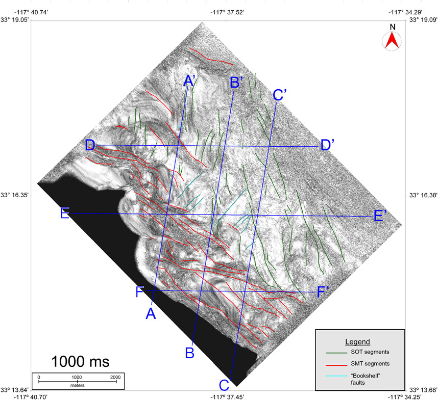
FIGURE 6. Time-slice view of sparker survey at 1,000 ms rendered using similarity attribute. White areas in the map show high similarity ( ∼ 1) and black areas low similarity ( ∼ 0). Interpreted fault segments are shown with solid lines and color-coded according to azimuth and character. Dark green faults trend northward, show steeply vertical dip and are within the San Onofre trend (SOT) fault zone. Red fault segments trend towards the northwest, exhibit transpressional features, and are within the San Mateo trend (SMT) fault zone. Light blue segments trend to the northeast and appear to accommodate rotation between the SOT and SMT fault zones. Dark blue lines with labels denote locations of the vertical seismic arbitrary lines shown in Figures 8 and 9. See location of the survey in Figures 4, 5.
Fault planes mapped by tracing the faults throughout the 3D seismic volume captures how the fault plane changes trends across the margin, along the margin, and with depth (Figure 7). Although in the time slice (Figure 6) SMT trends more to the northwest and SOT more northerly, the planes show that the trends exhibit minor variation with depth (Figure 7). In addition, the 3D geometry and distribution of the fault planes help image the different fault segments and how they structurally relate to adjacent faults. Strike slip faults with steep dips are usually not well imaged in 2D vertical sections; however, in 3D data volumes, fault terminations and changes in acoustic character are also imaged in time slices (e.g., map view; Figure 6). By examining faults in both vertical sections and in time slices, it further reduces the uncertainty of fault mapping, which increases the ability to define the fault architecture and the interaction between neighboring segments.
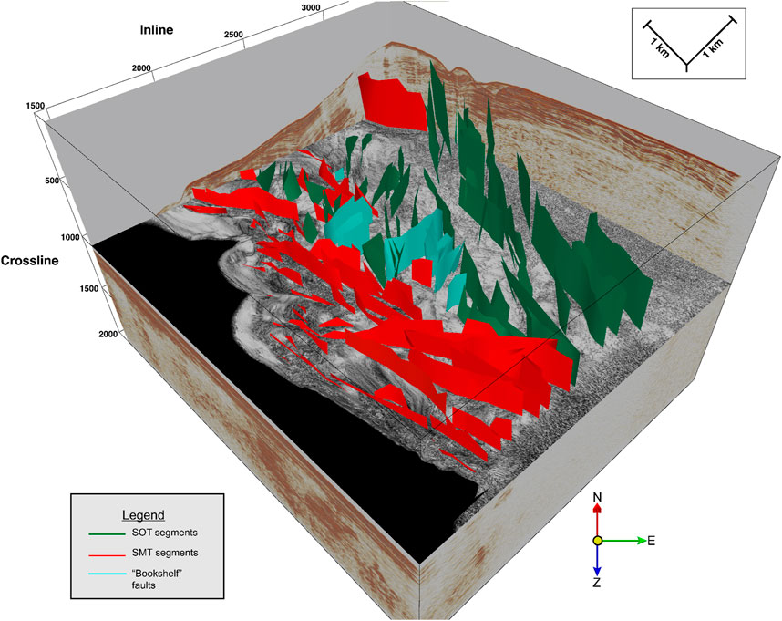
FIGURE 7. 3D chair view of sparker survey area. View is due north, oblique to the continental shelf. Dip line and strike line amplitude vertical profiles frame a timeslice at 1,000 ms rendered in similarity attribute. Green faults correspond to the San Onofre Trend (SOT) fault system and trend towards the continental shelf where they intersect with Newport-Inglewood Rose Canyon fault system. Red faults correspond to the San Mateo trend (SMT) fault system trending towards the northwest, subparallel to the continental margin. Light blue faults denote the bookshelf faults that trend to the northeast and appear to accommodate rotation between the SOT and SMT fault zones. See location of the survey in Figures 4, 5.
Arbitrary line transects were constructed from the 3D data volume approximately perpendicular to the SMT system (Figures 8A–C) and the SOT system (Figures 9A–C). In Figures 8A–C, 9A–C, there are differing vertical exaggerations in order to display the lines at the same widths despite varying seismic line lengths. We will first describe the dip sections from west to east. Arbitrary line A-A′ (Figures 5, 6, 8A) shows a change in the dip attitude of the imaged reflectors just to the northeast of cross-line D-D′. To the north of the profile the reflectors exhibit a slight dip to the southwest, show little signs of folding and the SOT faults do not reach the seafloor. In contrast, south of the northernmost SMT fault, the reflectors are folded and offset up to close to the seafloor. The line shows a broad antiform-synform pair and along the northeast limb of the anticline the reflectors are truncated at the seafloor. The north and south San Onofre Canyons are imaged on the northeast limb and crest of the anticline. The antiform-synform pair is bounded to the southwest by a fault system near cross-line E-E′. The entire survey area is characterized by zones of acoustic transparency possibly related to fluid content in the sedimentary units or fault shear (especially visible in Figure 9C). Reflector continuity increases toward the southwest, clearly showing that they are faulted and folded. At the boundary between the basin floor and the slope (Figures 8A–C, 9B,C), there is another fault system north of which the reflectors are also faulted and folded and show acoustically transparent zones. The larger SMT fault segments (mapped with thick red lines in Figures 8–10) show reverse vertical displacement.
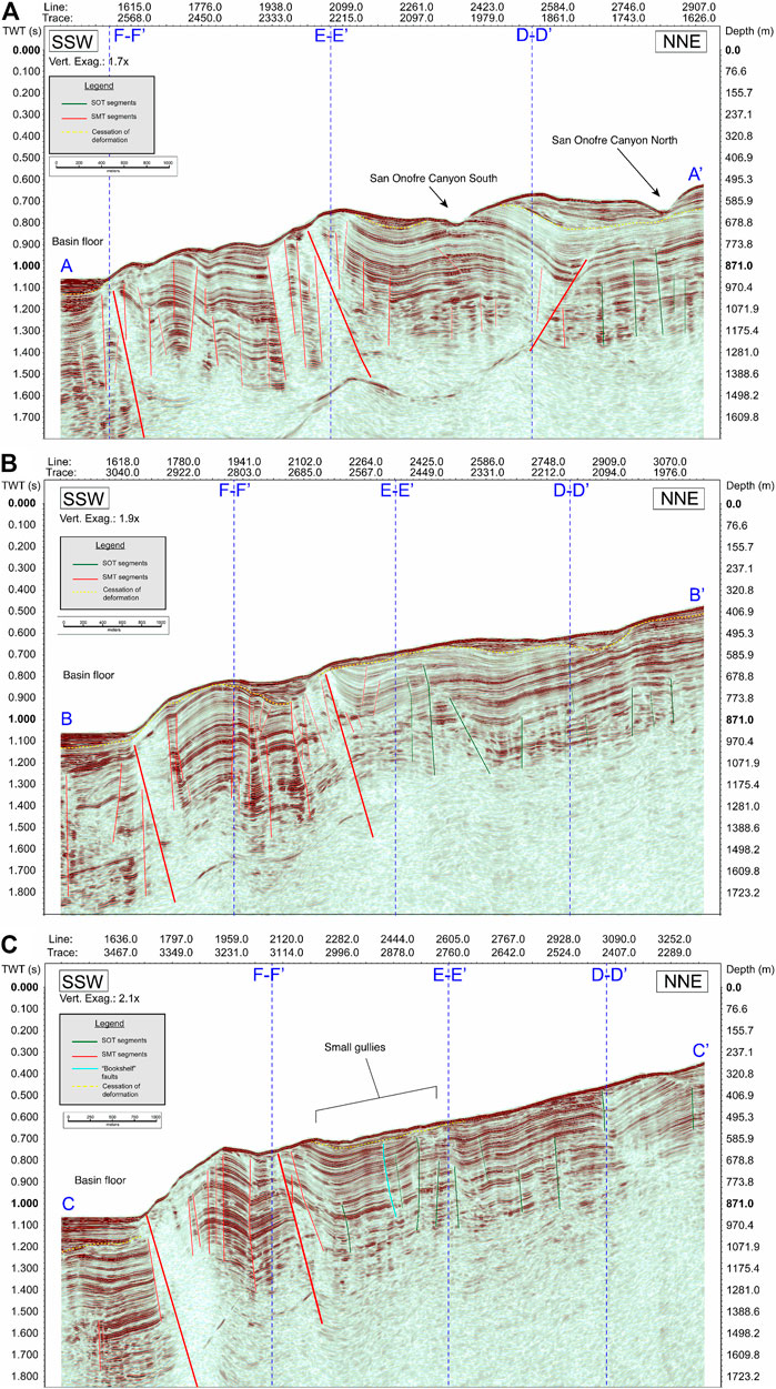
FIGURE 8. Vertical arbitrary seismic line sections rendered in amplitudes. Locations are shown in Figures 5, 6. (A) Dip line transect from A to A′, orthogonal to San Mateo Trend fault system (SMT). Vertical exaggeration is 1.7×. (B) Dip line transect from B to B′, orthogonal to SMT. Vertical exaggeration is 1.9×. (C) Dip line transect from C to C′, orthogonal to SMT. Vertical exaggeration is 2.1×. For all sections, faults are color-coded according to azimuth and character. Red faults correspond to SMT. Green faults correspond to the San Onofre Trend fault system (SOT). Minor fault segments (segments that cannot be mapped beyond 50 lines) shown with thin lines. Yellow dashed line marks base of sediment packages that represent cessation of deformation. Blue dashed lines show intersections with the vertical arbitrary seismic lines in Figures 9A–C.
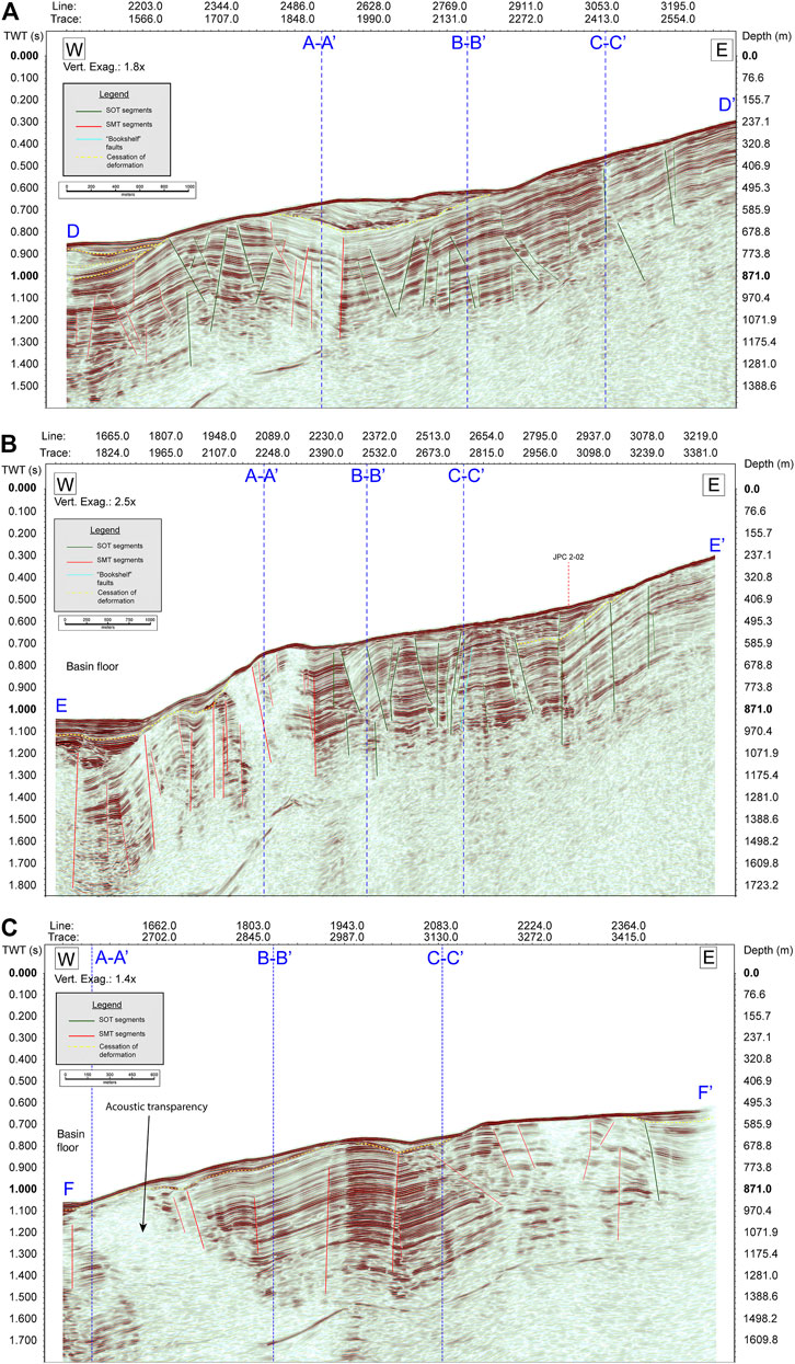
FIGURE 9. Vertical arbitrary seismic line sections rendered in amplitudes. Locations are shown in Figures 5, 6. (A) Dip line transect from D to D′, orthogonal to San Onofre Trend fault system (SOT). Vertical exaggeration is 1.8×. (B) Dip line transect from E to E′, orthogonal to SOT. Vertical exaggeration is 2.5×. (C) Dip line transect from F to F′, orthogonal to SOT. Vertical exaggeration is 1.4×. For all sections, faults are color-coded according to azimuth and character. Red faults correspond to San Mateo Trend fault system (SMT). Green faults correspond to the SOT. Minor fault segments (segments that cannot be mapped beyond 50 lines) shown with thin lines. Yellow dashed line marks base of sediment packages that represent cessation of deformation. Blue dashed lines show intersections with the vertical arbitrary seismic lines in Figures 8A–C. Short red dashed line in 9b denotes location of mid-slope jumbo piston core (JPC) 2–02.
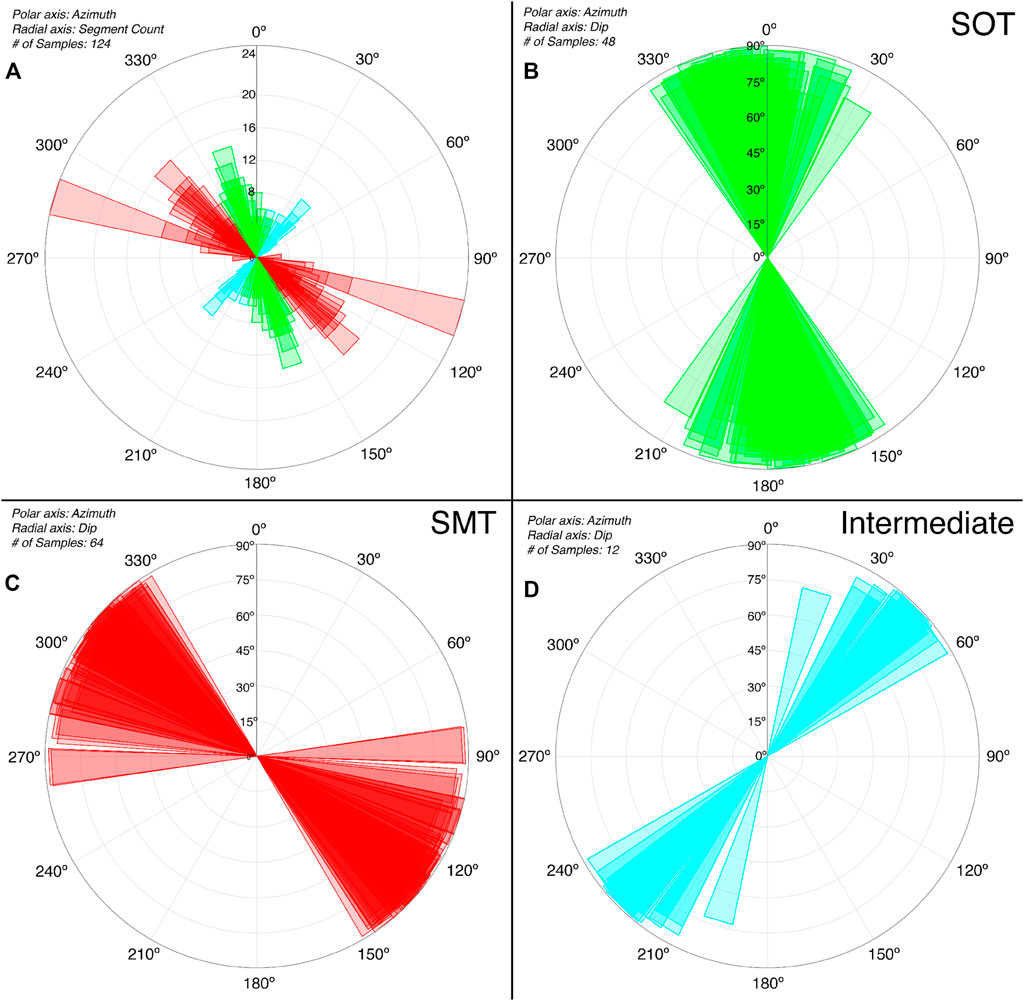
FIGURE 10. Rose diagrams of fault segments interpreted in the sparker survey data volume. (A) Azimuth vs. number of fault picks for all interpreted faults. Fault picks are on radial axis, azimuth is on polar axis. Picks were made every 50 lines, so unbroken fault length can be inferred on the radial axis. Fault segments were color-coded into three different categories depending on azimuth. Green faults correspond to the San Onofre trend (SOT). Red faults correspond to the San Mateo trend (SMT). Light blue faults denote the bookshelf faults that trend to the northeast and appear to accommodate rotation between the SOT and SMT fault zones. Fault segments lengths are largely consistent; however, SMT system contained the longest fault segments at the toe of slope. (B) Graph showing azimuth vs dip of segments categorized as belonging to the SOT. Measured fault dips ranged from 63.9° to 89.8° for 48 segments. (C) Graph showing azimuth vs. dip of segments categorized as belonging to the SMT. Measured fault dips ranged from 72.6° to 90° for 64 segments. (D) Graph showing azimuth vs. dip of segments categorized as belonging to the bookshelf faults. Measured fault dips ranged from 73° to 89.3° for 12 segments.
Arbitrary line B-B′ (Figures 5, 6, 8B), located to the east of line A-A′, shows again a change in reflectors dip attitude near crossline E-E′ (Figure 8B); however, the antiform-synform pair exhibits less amplitude than in line A-A′ (Figure 8A). Upturned reflectors are fault bounded to the southwest of the folded zone and appear truncated at the seafloor. Continuing southwest, a well-developed antiform is imaged with its crest near cross line F-F′. The northeastern limb is faulted and show smaller scale folds. Flat lying reflectors corresponding to the basin floor are separated from the southwestern limb of the antiform by a northeastward dipping fault mapped across an acoustically transparent zone (Figure 8B).
A change in the dip attitude of the reflectors is also imaged by arbitrary line C-C′ just to the northeast of cross-line F-F′ (Figure 8C). To the north the reflectors, even though they are faulted and folded, show a consistent dip towards the southwest. This dip trend ends in a zone characterized by a faulted synform-antiform-synform-antiform structure, from northeast to southwest; the folding is tighter toward the toe of the slope in this region than imaged on the arbitrary lines A-A′ and B-B′ (Figures 8A,B, respectively). An acoustically transparent zone separates the southernmost faulted anticline from the basin floor and the reflectors display a marked change in dip across this zone. We have mapped a northwest dipping fault across this zone considering the change in attitude of the reflectors on either side of an acoustically transparent zone and according to our interpretations on the other dip sections (Figures 8A,B).
The northernmost arbitrary line orthogonal to SOT (D-D’; Figure 9A) images two different zones with the change between them occurring east of cross-line A-A′. To the east of the line, the reflectors are more continuous, dip to the west and the faults accommodate short displacements; to the west, the line shows a large anticline with several faults in the axial zone that offset reflectors close to the seafloor. Onlapping reflectors are observed toward the west of the large anticline. A wedge-shaped unit of truncated reflectors infills the structural low where the deeper reflectors change the attitude of dip, just between crosslines A-A′ and B-B′. SOT fault segments imaged in this line display normal and reverse displacements.
Arbitrary line E-E′, to the south, shows that the deformation is spread over a broader area with reflectors mainly dipping to the west (Figure 9B); however, there is a decrease in reflector dip moving from the margin and west of the location of core JP 2–02 and then an increase from east of cross-line A-A′ and up to the basin floor, where also the bathymetric slope increases. This last zone of westward dipping reflectors also shows faulting and folding, and large acoustically transparent zones. On the basin floor area, there is a package of acoustically laminated reflectors that onlap the faulted and folded unit.
Finally, the southernmost arbitrary line F-F′ also shows the regional change in dip attitude (Figure 8B), but more subtle than in the previous sections. A broad antiform is imaged in the central portion of the profile, between crosslines B-B′ and C-C′. The antiform is bounded to the east by a SMT fault segment with little vertical reverse displacement. To the east and west of the anticline the line shows more acoustically transparent regions introducing uncertainty to the interpretation.
Rose diagrams were generated to display the fault trends and dips in the 3D seismic data volume (Figure 10). Three main fault trends emerge from the rose diagram analysis (Figure 10A), which is in agreement with the 3D seismic interpretation (Figures 6, 7). The SMT faults (Figures 10A,C) shows two predominant azimuths, the principal of ∼ 285° and the secondary of ∼ 310°, with an average around azimuth 300°. In contrast, the SOT faults (Figures 10A,B) trend more northerly with an average azimuth of ∼ 345°. Finally, the smaller intermediate faults (Figures 10A,D) also present a main trend direction with an average azimuth of ∼ 40°, approximately orthogonal to SMT and SOT systems. The analysis of the fault dips on the rose diagrams reveals that most of the faults mapped in the 3D volume are steep faults with dips ranging between 64° to 90°and clear predominance of faults dipping between 80 and 90° (Figures 10B–D). These steep dips observed in the 3D P-Cable data are also observed in MCS data along the margin (Figure 11).
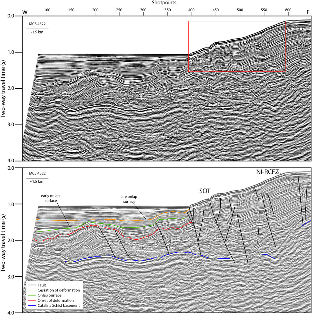
FIGURE 11. Un-interpreted (top) and interpreted (bottom), re-processed MCS line 4522 modified from Maloney et al., 2016. Much of the character of the San Onofre Trend (SOT) is shown here as steeply dipping faults to the east that terminate at or near a horizon interpreted as Catalina Schist basement. Red box in upper image shows lateral extent of the survey and vertical extent of interpretations presented in this paper. Profile location is shown in Figure 5. Abbreviations: SOT, San Onofre trend; NI-RCFZ, Newport Inglewood-Rose Canyon fault zone.
The high-resolution bathymetry computed from the amplitude of the 3D seismic data volumes show the influence of the SMT and SOT on the gullies and seafloor morphology (Figure 12). The area south of the San Onofre canyons is dominated by several small gullies trending ENE-WSW (Figures 8C, 12). These gullies are more subtle or even disappear in an area in between two locally uplifted regions and where two morphological scarps trending approximately N-S are observed (Figure 12). The trend of these scarps is consistent with the trend of the SOT faults and the uplifted regions are localized close to fault segments that show left lateral jogs (Figure 12B). At the toe of slope, there are large, deformed ridges with a mounded morphology, bounded by faults of the SMT system, but they appear to be oriented more toward the northwest in comparison to the bounding faults (Figure 12). The bathymetry also shows that the boundary between these mounded features and the basin floor is extremely steep dipping at almost 25° (Figure 4) and that there is rather abrupt change in the seafloor morphology between the SOT and SMT dominant areas (Figure 12). Finally, there are two subtle uplifted zones and a sigmoid gully in the boundary area between that SOT and SMT systems that appears to be controlled by the activity of one of the smaller intermediate faults (Figure 12).
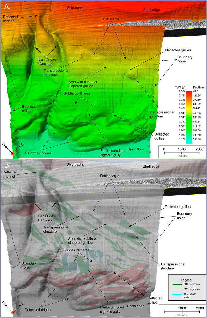
FIGURE 12. (A) Depth-colored map view of seafloor bathymetry computed from 3D seismic data amplitude volumes. Continental margin is towards the top of image (red colors). Toe of slope is largely deformed at the interface with the basin floor (green colors). Transpressional structures, gullies and canyons appear offset or diverted by fault scarps at the seafloor. (B) Map view of seafloor bathymetry colored in shades of gray and 20% transparent. 3D fault planes are plotted below seafloor and color-coded according to strike and character. Green faults correspond to the San Onofre trend (SOT). Red faults correspond to the San Mateo trend (SMT). Light blue faults denote the bookshelf faults that trend to the northeast and appear to accommodate rotation between the SOT and SMT fault zones. See location of the survey areas in Figures 4, 5.
Discussion
Deformation, Sediment Transport and Margin Morphology
The slope offshore San Onofre, where the 3D sparker data were acquired, appears to be less well incised by canyon systems than the slopes directly north and south of the area (Figure 4). In addition, the seafloor shows features with a mounded morphology close to the transition from the slope to the basin floor, which also presents high slope angles (25°) at the toe of the continental slope (Figures 4, 5, 12). In contrast, the slopes to the north and south along the margin exhibit more regular surfaces and a gradual transition from the toe of the slope to the basin floor (Figures 4, 5, 12). Previous studies have shown that the wide shelf offshore San Onofre (Figure 2) is spatially coincident with a large anticline related to a left lateral jog in the NIRC and suggest that this anticline may act as a barrier to sediment traversing the inner shelf up to the basin floor in this area (Sahakian et al., 2017; Wei et al., 2020; Holmes et al., 2021). The lack of sediments dispersal in this region of the slope may explain the almost absence of well-developed channels along the studied area. In addition, the activity on the SOT and SMT faults have produced small changes in slope and depressions where the few traversing sediments may be trapped and not reaching the lower parts of the continental slope (Figures 8A–C, 9A–C). Thus, the almost unavailability of sediments at the lower parts of the continental slope may explain the clear surface morphology of the mounded features and the high slope angles at the toe of the continental slope, both related to fault activity (Figure 11). In addition, this may also account for the differences between this area and the other areas along the margin (Figure 1). According to all the observations, the lateral superposition in the same area of the NIRC and the SOT and SMT systems seems to control the sediment supply and distribution from the continental shelf to the continental slope and the morphology of the slope.
The continental shelf along the southern California margin from Palos Verdes (“PV”) to La Jolla exhibits marked variability (Figures 1, 2). The wider portions of the shelf north of La Jolla Canyon (Hogarth et al., 2007; LeDantec et al., 2010), San Onofre (Sahakian et al., 2017; Holmes et al., 2021) and south of Palos Verdes are regions where left lateral jogs occur along the predominantly right lateral fault systems offshore (Figure 1). Left lateral jogs along right lateral strike slip faults engenders transpression, often referred to as restraining bends (Cunningham and Mann, 2007). In contrast, a right lateral jog along a right lateral strike slip fault system creates transtension. The wide shelf offshore San Onofre is spatially coincident with a large anticline formed in a left lateral jog in the NIRC in the area where this system coincides with the SOT and SMT. The littoral sediment transport along the southern California shelf is southwards (LeDantec et al., 2010). Thus, the widening of the self in the San Onofre margin may be related with the anticline formed in the NIRC impeding the sediment traversing the inner shelf and diverting the sediment transport to the south (Wei et al., 2020; Holmes et al., 2021). Southwards of San Onofre the sediments appear to be trapped and transferred to the deeper areas by the Oceanside and Carlsbad canyons (OC and CC in Figure 1). Both canyons exhibit a more sinuous nature than the more linear canyons to the north and their canyon heads intersect the shelf. From this point, the width of the shelf diminishes rapidly from north to south (Figures 1, 2). According to these observations, the absence of tectonically uplifted areas (i.e., restraining bends or anticlines) allows the sediment transported along-shore to intersect the shelf edge as the shelf width diminishes and this might explain the location and morphology of the Oceanside and Carlsbad canyons. In a similar manner, sediment is shunted offshore into La Jolla Canyon due to the uplift of Mount Soledad (MS in Figure 1), which acts as a natural jetty to southerly sediment transport. In addition, the sinuous morphology of these canyons (e.g., La Jolla, Carlsbad and Oceanside) appears to occur where along-shore transport intersects the shelf edge and spawn gravity flows that sculpt and shape the canyons.
Age of the Deformation
Constraining the relative age of deformation is difficult as the present-day seafloor exhibits erosional and structural truncation resulting from slumping, block rotation and downslope canyon erosion. Nevertheless, flat lying deposits on the basin floor appear to onlap the deformation structures and suggest the deformation there may have ceased (Figures 8A–C, 9B); an interpretation that is consistent with previous studies (Maloney et al., 2016). We measured the thickness of basin floor turbidites imaged on the arbitrary lines A-A′ (53.6 m at trace 2661), B-B′ (46.0 m at trace 3123) and C-C′ (91.9 m at trace 3473) (Figures 8A–C). Using the estimated sedimentation rate of 0.25 mm/yr, we obtain that the activity in the SMT fault system may have ended between 184 and 368 kyr ago. Establishing the cessation of activity in the SOT system is not possible since there is no information to determine the age of the non-offset reflectors. Comparing the depth of the reflectors offset by SMT and SOT fault systems, which is similar (Figures 8A–C, 9A–C), it seems plausible to consider that the deformation in the SOT may have ended around the same time range obtained for SMT. Nevertheless, the presence of possible fault-related scarps offsetting the seafloor and associated with the SMT faults (Figure 12) suggest that some of the faults could still be active, maybe as splays off the NIRC system.
Left Lateral Jog Deformation Versus Thrust Deformation
The San Mateo trend (SMT), San Onofre trend (SOT), are mapped west of the Newport-Inglewood-Rose Canyon fault zone, offshore from San Onofre, whereas the Carlsbad trend (CT) extends farther south and terminates offshore north of Del Mar (Figure 1). These trends have been identified as active structures that produce bathymetric relief on the seafloor (Rivero and Shaw, 2011; Maloney et al., 2016). Two alternative interpretations may explain the formation and evolution of SMT, SOT and CT. The first interpretation suggests that these faults could be forethrusts soling into the Oceanside blind thrust (OBT) at depth and the associated folding (anticlines and faulted anticlines) fault-related and fault-propagation folds (Rivero et al., 2000; Rivero and Shaw, 2011). The second interpretation proposes that these trends may accommodate transpression associated with jogs along the NIRC strike-slip fault zone (Crouch and Bachman, 1989; Fischer and Mills, 1991; Ryan et al., 2009; Maloney et al., 2016) with potential large block rotation bounded by strike-slip faults (Ryan et al., 2009; Ryan et al., 2012).
The arbitrary north-northeast strike lines, almost orthogonal to the SMT (i.e., A-A′, B-B′, and C-C′; Figures 5, 6, 8A–C), show that the main compressional faulting and folding structures are related to the activity in the SMT faults. These lines image an anticline-syncline pair near the toe of the slope with the width of the fold diminishing towards the east (Figure 8). Arbitrary east-west strike lines (i.e., D-D′, E-E′ and F-F′; Figures 5, 6, 9A–C) are more subparallel to the SMT faults and folds, thus the apparent wavelength of the deformation appears longer. Note that along the arbitrary north-northeast strike lines (Figure 8) there are large dominant northeast dipping faults that bound the regional deformation and subordinate faults that appear to accommodate the more localized deformation. These large faults extend close to the seafloor; however, there is no clear seafloor offset across the faults. We interpret the anticlines as related to shortening produced by different restraining step-overs or bends. The change in direction of a fault, or areas between faults, can experience shortening that results in the formation of anticlines and synclines (Mann, 2007; Dooley and Schreurs, 2012). Also, close to the toe of the slope there are the NW trending mounded features that measure 2–4 km in length and 1–2 km in width (Figures 4, 12). These features are very localized along the margin and occur where there is marked left lateral jogs along the SMT faults (Figures 6, 12). Accordingly, these observations appear to support the hypothesis that the faults in the area are accommodating transpression associated with strike-slip faulting instead of regional thrust faulting. In addition, although the area covered by the 3D seismic data volume is very localized with a lateral extent of approximately 12 km, it clearly shows the compressional features are localized. Interpretation of the new 3D P-Cable data reveals that the faults are quite segmented with clear step-overs between them (Figures 6, 7, 12).
The 3D seismic dataset images the upper few kilometers of the seismostratigraphic succession at very high resolution but does image the fault geometry at depth. Maloney et al. (2016) presented reprocessed multi-channel seismic (MCS) lines collected offshore of the southern California coast from Dana Point to Oceanside. MCS line 4522 (Figure 11) is a dip line that crosses through the southeastern third of our survey area (Figure 5) and crosses several splays of the SOT. High quality MCS provides deeper context for fault interpretations. In this case, faults are imaged down to 4 s TWTT. Interpreted faults are observed to be steeply dipping, generally towards the east, and terminate at or near a horizon interpreted as Catalina Schist basement rock. A possible offset in Catalina Schist is mapped at depth below the continental shelf to slope transition (Maloney et al., 2016). Accordingly, the steep vertical faults mapped in the 3D dataset appear to be steeply dipping at depth where they intersect the Catalina Schist. As pointed out by Maloney et al. (2016), an offset of the acoustic basement (i.e., Catalina Schist) is difficult to reconcile with the interpreted OBT.
Regionally, Global Navigation Satellite System (GNSS) data shows plate velocity vectors moving northwestward with respect to a fixed North America, with an average azimuth around 313° (Figure 1). This direction is slightly oblique to the strike of most of the strike-slip faults in the ICB, and almost parallel to both the Thirtymile Bank and the southern part of the Oceanside blind thrusts (TBBT and OBT in Figure 1). The focal mechanisms for earthquakes with magnitude above 4.5 show a mixture between strike-slip and reverse fault solutions. Both types of focal mechanism show at least one of the nodal planes trending parallel to the main fault systems in the ICB. In the case of the strike slip solutions, the other nodal plane tends to trend perpendicular to these fault systems. Even the focal mechanism of the 1986 M5.3 Oceanside earthquake corresponds to a reverse fault solution, the earthquake and aftershocks have been associated with the San Diego Trough strike-slip fault (Ryan et al., 2012) (Figure 1). The rose plot of segment count vs azimuth (Figure 10A) shows that SOT faults have a predominant strike around 345° whereas faults in the SMT show a main strike around 285° and a second family with strikes around 310°. The comparison of the GNSS velocity vectors with the azimuth of the faults in the SOT and SMT systems may also explain the different vertical displacement accommodated in both fault systems. As shown in the interpretation of the 3D dataset, the area where the SOT faults are localized shows less folding and vertical deformation than the area at the toe of the slope where the SMT faults are associated with mounded morphologies and anticline-syncline pairs (Figures 6, 8, 9, 12). In general, GNSS and focal mechanisms suggests that the ICB is subject to transpressional kinematics, with reverse kinematics associated mainly to step-overs between the main strike-slip fault systems. The observed change from transtension to transpression observed along slope may also be related to a large gravity slide but given the lack of extensional features on the shelf (Holmes et al., 2021), our preferred model for the deformation along the SMT and SOT is best explained by left lateral step-overs along the predominantly right lateral strike-slip fault systems.
The high-resolution bathymetry derived from the 3D seismic volume (Figure 12) shows the presence of two geomorphological scarps and two local highs, which appear to deflect gullies in the center of the area where the SOT faults are predominant. The comparison with the different identified SOT faults shows that the scarps are fault related and that the highs may correspond to compression pop-ups occurring along left lateral fault jogs (Figure 12B). Towards the north, the SOT faults appear to connect with faults related to the NIRC system and mapped along the shelf edge in the 3D boomer data (Holmes et al., 2021). According to these observations, we suggest that the SOT faults along the slope may mark the termination of the Camp Pendleton splay of the Newport-Inglewood Fault (Figure 5) as the deformation is deflected westward away from the zone of compression on the shelf. The lack of deformation and offset of the transgressive surface imaged in CHIRP seismic data acquired on the continental shelf in this region (Klotsko et al., 2015; Sahakian et al., 2017; Holmes et al., 2021) is also consistent with the strike-slip hypothesis.
In the transition zone between the SMT and SOT fault systems, short NE-SW trending faults have been mapped (Figures 6, 7, 12). Most of these faults show normal displacement, with the total vertical offset much less then that shown by the main faults in the SMT and SOT systems (Figures 8C, 9B). We suggest that these NE-SW faults may have accommodated the differential displacement between the two major fault systems by transtension. In general, northeast of the transition zone the reflectors dip towards the basin and are continuous and mainly plane-parallel, although show some minor folding mainly related to SOT faults. Rivero et al. (2000) interpreted that the dip of these reflectors may partially be the result of shortening above an underlying detachment. Any regional shortening in the area may result in tilting or generation of large amplitude folding. Regional folding is not observed in the dataset. Any tilting, however, would result in the formation of angular unconformities, onlap geometries, and growth strata towards the basin are not observed in the 3D dataset. There is no evidence for any tilting in the area and thus, we assume that the dip of the reflectors corresponds to sedimentary deposition. Some similar structures have been observed in analog modelling experiments as related to gravitational processes (Richard and Krantz, 1991), however the analysis of the dataset and the tectonic environment leads us to interpret the deformation in the slope as being related to active faulting, as seen in other areas of the ICB (Maloney et al., 2016; Sahakian et al., 2017).
To sum up, all the observations based on the analysis of the 3D sparker seismic data suggest that the fault systems along and across the San Onofre margin appear to be accommodating transpressional deformation, which is consistent with analysis of the GNSS data and the focal mechanisms. Thus, our results appear to support the hypothesis that the SMT and SOT systems along the ICB margin are accommodating transpression associated with jogs along NIRC fault zone.
Conclusion
Newly acquired 3D P-Cable MCS and bathymetry data along the slope offshore southern California place important constraints on the architecture of the SOT and SMT. Conceptual models to explain the offshore deformation need to consider the following observations:
1) Mounded, bulbous morphology with steep slopes ( ∼ 25°) are observed at the boundary between the toe of the slope and the basin floor; the deformation is very localized. The style and magnitude of the deformation is greatest along the SMT and dies away toward the north/northeast.
2) The steeply dipping faults in the SMT and the SOT exhibit markedly different trends and the boundary between the two trends is abrupt.
3) Localized compression in the SOT occurs as predicted at fault bends and step-overs (i.e., un-named faults). The transpressional features are observed in the swath bathymetry data and appear to deflect canyons/gullies along the slope.
4) The SOT faults on the slope appear to be splays off the Newport Inglewood fault mapped on the shelf.
5) Shorter faults recording right-lateral displacement with an average trend of ∼ 40° are observed in the boundary zone between the SMT and SOT. They may be acting to accommodate displacement between the larger fault systems.
6) The lack of deformation in the flat lying onlapping sequences suggest that the activity in the SMT and SOT systems may have ceased between 184 and 368 kyr ago.
In summary, the timing and style of deformation observed in the SOT and SMT are better explained by left lateral jogs along right lateral fault systems that engenders transpression than splays off a master regional detachment (i.e., OBT).
Data Availability Statement
The original contributions presented in the study are included in the article/Supplementary Materials, further inquiries can be directed to the corresponding author.
Author Contributions
JH wrote the manuscript and created figures. HP cowrote the manuscript and provided substantial edits. ND and GK provided guidance, manuscript edits, and project funding.
Funding
Funding for this research was provided by a grant from Southern California Edison funded through the California Public Utility Commission (CPUC), and the Maxwell J. Fenmore Memorial Fellowship. HP was supported by the European Union’s Horizon 2020 research and innovation program under grant H2020-MSCA-IF-2014 657769 and by the Madrid Community’s “Atracción de Talento Investigador” call 2018 program under the grant 2018-T1/AMB-11039.
Conflict of Interest
The authors declare that the research was conducted in the absence of any commercial or financial relationships that could be construed as a potential conflict of interest.
The reviewer JS declared a past co-authorship with several of the authors HP, ND, GK to the handling editor.
Publisher’s Note
All claims expressed in this article are solely those of the authors and do not necessarily represent those of their affiliated organizations, or those of the publisher, the editors and the reviewers. Any product that may be evaluated in this article, orclaim that may be made by its manufacturer, is not guaranteed or endorsed by the publisher.
Acknowledgments
The authors wish to acknowledge the assistance of Mike Barth of Subseas Systems, the sailing and science crews of the R/V New Horizon (NH1320, & NH1323) and R/V Thomas G. Thompson (TN336), Geotrace Technologies, and NCS Subsea, Inc. for their roles in data acquisition and processing. We would also like to thank Emily Wei for her assistance in core processing and analysis. Figures were generated using Generic Mapping Tools, version 5 (Wessel et al., 2013), Kingdom Suite 2019 (IHS Markit), and OpendTect 6.4.4 (dGB Earth Sciences). Cruise information for NH1320 (2D MCS; https://doi.org/10.7284/902996), NH1323 (3D P-Cable MCS; https://doi.org/10.7284/903024), and TN336 (Coring; https://doi.org/10.7284/906644) are accessible via the Rolling Deck to Repository (R2R) web interface. Seismic data are archived with Marine Geoscience Data System repository.
Supplementary Material
The Supplementary Material for this article can be found online at: https://www.frontiersin.org/articles/10.3389/feart.2021.653366/full#supplementary-material
Supplemental Figure S1 | (A) Example crossline from continental shelf survey shown after industry processing but before noise removal. The same procedure was employed on the continental slope survey described in this paper. (B) Vertical profile showing combined original seismic amplitudes and dip component at crossline. Dip in all directions was used as a steering parameter of the filter. Note that dip was automatically computed on low amplitude artifacts above the seafloor. These artifacts are due to ringing from the post-migration dip filtering process. (C) Profile of noise removed from crossline after applying a dip-steered median filter. Filter parameters were adjusted to minimize the amount of primary energy removed. (D) Crossline after application of filter. More continuous reflections are now observed.
References
Atwater, T., and Stock, J. (1998). Pacific-North America Plate Tectonics of the Neogene Southwestern United States: An Update. Int. Geology. Rev. 40 (5), 375–402. doi:10.1080/00206819809465216
Bahorich, M., and Farmer, S. (1995). 3-D Seismic Discontinuity for Faults and Stratigraphic Features: The Coherence Cube. The Leading Edge. 14 (10), 1053–1058. doi:10.1190/1.1437077
Bennett, R. A., Rodi, W., and Reilinger, R. E. (1996). Global Positioning System Constraints on Fault Slip Rates in Southern California and Northern Baja, Mexico. J. Geophys. Res. 101 (B10), 21943–21960. doi:10.1029/96JB02488
Blaauw, M., and Christen, J. A. (2011). Flexible Paleoclimate Age-Depth Models Using an Autoregressive Gamma Process. Bayesian Anal. 6, 457–474. doi:10.1214/11-BA61810.1214/ba/1339616472
Bohannon, R. G., and Parsons, T. (1995). Tectonic Implications of Post-30 Ma Pacific and North American Relative Plate Motions. Geol. Soc. America Bull. 107 (8), 937–0959. doi:10.1130/0016-7606(1995)107<0937:tiopmp>2.3.co;2
Brookshire, B. N., Lippus, C., Parish, A., Mattox, B., and Burks, A. (2016). Dense Arrays of Short Streamers for Ultrahigh-Resolution 3D Seismic Imaging. The Leading Edge. 35 (7), 594–599. doi:10.1190/tle35070594.1
Brothers, D. S., Conrad, J. E., Maier, K. L., Paull, C. K., McGann, M., and Caress, D. W. (2015). The Palos Verdes Fault Offshore Southern California: Late Pleistocene to Present Tectonic Geomorphology, Seascape Evolution, and Slip Rate Estimate Based on AUV and ROV Surveys. J. Geophys. Res. Solid Earth. 120, 4734–4758. doi:10.1002/2015JB011938
Conrad, J. E., Brothers, D. S., Maier, K. L., Ryan, H. F., Dartnell, P., and Sliter, R. W. (2019). Right‐Lateral Fault Motion Along the Slope‐Basin Transition, Gulf of Santa Catalina, Southern California. Mountains Abyss: Calif. Borderland as Archive South. Calif. Geologic Evol. Spec. Publ. 110, 256–272. doi:10.2110/sepmsp.110.07
Covault, J. A., Romans, B. W., Fildani, A., McGann, M., and Graham, S. A. (2010). Rapid Climatic Signal Propagation From Source to Sink in a Southern California Sediment‐Routing System. J. Geology. 118 (3), 247–259. doi:10.1086/651539
Crouch, J. K., and Bachman, S. B. (1989). Exploration Potential of the Offshore Newport-Inglewood Fault Zone. AAPG Bull. 73, 536. doi:10.1306/44b4a05f-170a-11d7-8645000102c1865d
Crouch, J. K., and Suppe, J. (1993). Late Cenozoic Tectonic Evolution of the Los Angeles Basin and Inner California Borderland: A Model for Core Complex-like Crustal Extension. Geol. Soc. America Bull. 105 (11), 1415–1434. doi:10.1130/0016-7606(1993)105<1415:lcteot>2.3.co;2
Crutchley, G. J., and Kopp, H. (2018). “Reflection and Refraction Seismic Methods,” in Submarine Geomorphology. Editors A. Micallef, S. Krastel, and A. Savini (Cham: Springer Geology. Springer). doi:10.1007/978-3-319-57852-1_4
Cunningham, W. D., and Mann, P. (2007). Tectonics of Strike-Slip Restraining and Releasing Bends. Geol. Soc. Lond. Spec. Publications. 290, 1–12. doi:10.1144/SP290.1
Dartnell, P., Driscoll, N. W., Brothers, D. S., Conrad, J. E., Kluesner, J., Kent, G., et al. (2015). Colored Shaded-Relief Bathymetry, Acoustic Backscatter, and Selected Perspective Views of the Inner Continental Borderland, Southern California. US Geol. Surv. Scientific Invest. Map. 3324 (3). doi:10.3133/sim3324
Dooley, T. P., and Schreurs, G. (2012). Analogue Modelling of Intraplate Strike-Slip Tectonics: A Review and New Experimental Results. Tectonophysics. 574-575, 1–71. doi:10.1016/j.tecto.2012.05.030
Ebuna, D. R., Mitchell, T. J., Hogan, P. J., Nishenko, S., and Greene, H. G. (2013). “March). High-Resolution Offshore 3D Seismic Geophysical Studies of Infrastructure Geohazards,” in Symposium on the Application of Geophysics to Engineering and Environmental Problems 2013 (Society of Exploration Geophysicists and Environment and Engineering Geophysical Society), 311–320.
Eriksen, F. N., Berndt, C., Karstens, J., and Crutchley, G. J. (2015). “P-Cable High Resolution 3D Seismic-Case Study and Recent Advances,” in Near-Surface Asia Pacific Conference, Waikoloa (Hawaii: Society of Exploration Geophysicists, Australian Society of Exploration Geophysicists, Chinese Geophysical Society, Korean Society of Earth and Exploration Geophysicists, and Society of Exploration Geophysicists of Japan), 116–119.
Fischer, P. J., and Mills, G. I. (1991). The Offshore Newport-Inglewood-Rose Canyon Fault Zone, California: Structure, Segmentation, and Tectonics. Environmental Perils. San Diego Region: San Diego Association of Geologists for Geologic Society of America Meeting, 17–36.
Freeman, S. T., Heath, E. G., Guptill, P. D., and Waggoner, J. T. (1992). “Seismic Hazard Assessment, Newport-Inglewood Fault Zone,” in Engineering Geology Practice in Southern California. Editors B. W. Pipkin, and R. J. Proctor (Belmont, CA: Association of Engineering Geologists Special Publication) 4, 211–229.
Grant, L. B., and Shearer, P. M. (2004). Activity of the Offshore Newport-Inglewood Rose Canyon Fault Zone, Coastal Southern California, From Relocated Microseismicity. Bull. Seismological Soc. America. 94 (2), 747–752. doi:10.1785/0120030149
Grant, L. B., Waggoner, J. T., Rockwell, T. K., and von Stein, C. (1997). Paleoseismicity of the North Branch of the Newport-Inglewood Fault Zone in Huntington Beach, California, From Cone Penetrometer Test Data. Bull. Seismological Soc. America. 87 (2), 277–293. doi:10.1785/BSSA0870020277
Hill, M. (1971). Newport-Inglewood Zone and Mesozoic Subduction, California. GSA Bull. 82 (10), 2957–2962. doi:10.1130/0016-7606(1971)82[2957:NZAMSC]2.0.CO;2
Hogarth, L. J., Babcock, J., Driscoll, N. W., Le Dantec, N., Haas, J. K., Inman, D. L., et al. (2007). Long-term Tectonic Control on Holocene Shelf Sedimentation Offshore La Jolla, California. Geology 35 (3), 275–278. doi:10.1130/G23234a.1
Holmes, J. J., Driscoll, N. W., and Kent, G. M. (2021). High-Resolution 3D Seismic Imaging of Fault Interaction and Deformation Offshore San Onofre, California. Front. Earth Sci. 9, 653672. doi:10.3389/feart.2021.653672
Kienast, S. S., and McKay, J. L. (2001). Sea Surface Temperatures in the Subarctic Northeast Pacific Reflect Millennial-Scale Climate Oscillations During the Last 16 Kyrs. Geophys. Res. Lett. 28, 1563–1566. doi:10.1029/2000GL012543
Klotsko, S., Driscoll, N., Kent, G., and Brothers, D. (2015). Continental Shelf Morphology and Stratigraphy Offshore San Onofre, California: The Interplay between Rates of Eustatic Change and Sediment Supply. Mar. Geology. 369, 116–126. doi:10.1016/j.margeo.2015.08.003
Kluesner, J. W., and Brothers, D. S. (2016). Seismic Attribute Detection of Faults and Fluid Pathways Within an Active Strike-Slip Shear Zone: New Insights from High-Resolution 3D P-Cable Seismic Data along the Hosgri Fault, Offshore California Seismic Data along the Hosgri Fault, Offshore California. Interpretation. 4 (1), SB131–SB148. doi:10.1190/INT-2015-0143.1
Kovanen, D. J., and Easterbrook, D. J. (2002). Paleodeviations of Radiocarbon Marine Reservoir Values for the Northeast Pacific. Geology. 30, 243–246. doi:10.1130/0091-7613(2002)030<0243:PORMRV>2.0.CO;2
Le Dantec, N., Hogarth, L. J., Driscoll, N. W., Babcock, J., Barnhardt, W. A., Schwab, W. C., et al. (2010). Tectonic Controls on Nearshore Sediment Accumulation and Submarine Canyon Morphology Offshore La Jolla, Southern California. Marine Geology 268 (1–4), 115–128. doi:10.1016/j.margeo.2009.10.026
Legg, M. R., and Kennedy, M. P. (1979). Faulting Offshore San Diego and Northern Baja California. Earthquakes and Other Perils, San Diego Region. San Diego, CA: San Diego Assoc. of Geologists, 29–46.
Lindvall, S. C., and Rockwell, T. K. (1995). Holocene Activity of the Rose Canyon Fault Zone in San Diego, California. J. Geophys. Res. 100 (B12), 24121–24132. doi:10.1029/95JB02627
Lonsdale, P. (1991). “Structural Patterns of the Pacific Floor Offshore of Peninsular California,” in Gulf and Peninsular Province of the Califor- Nias: American Association of Petroleum Geologists Memoir. Editors J. P. Dauphin, and B. R. T. Simoneit, 47, 87–143. doi:10.1306/m47542c7
Luyendyk, B. P., Kamerling, M. J., Terres, R. R., and Hornafius, J. S. (1985). Simple Shear of Southern California during Neogene Time Suggested by Paleomagnetic Declinations. J. Geophys. Res. 90 (B14), 12454–12466. doi:10.1029/jb090ib14p12454
Maloney, J. M., Driscoll, N. W., Kent, G. M., Bormann, J., Duke, S., and Freeman, T. (2016). “Segmentation and Step-Overs along Strike-Slip Fault Systems in the Inner California Borderlands: Implications for Fault Architecture and Basin Formation,” in Applied Geology in California. Editors R. Anderson, and H. Ferriz (New York, NY: Star Publishing), 655–677.
Mann, P. (2007). Global Catalogue, Classification and Tectonic Origins of Restraining-and Releasing Bends on Active and Ancient Strike-Slip Fault Systems. Geol. Soc. Lond. Spec. Publications. 290 (1), 13–142. doi:10.1144/SP290.2
Mineral Management Service (MMS) (1997). Oceanside Seismic Data Set. Washington, D.C.: U.S. Department of the Interior. Pacific Outer Continental Shelf CD97-01.
Moody, J. D., and Hill, M. J. (1956). Wrench-fault Tectonics. Geol. Soc. America Bull. 67 (9), 1207–1246. doi:10.1130/0016-7606(1956)67[1207:wt]2.0.co;2
Nicholson, C., Sorlien, C. C., Atwater, T., Crowell, J. C., and Luyendyk, B. P. (1994). Microplate Capture, Rotation of the Western Transverse Ranges, and Initiation of the San Andreas Transform as a Low-Angle Fault System. Geol. 22 (6), 491–495. doi:10.1130/0091-7613(1994)022<0491:mcrotw>2.3.co;2
Planke, S., Berndt, C., Mienert, J., and Bünz, S. (2009a). P-Cable: High-Resolution 3D Seismic Acquisition Technology. INVEST. 2009 Workshop. 23, 25.
Planke, S., Erikson, F. N., Berndt, C., Mienert, J., and Masson, D. (2009b). P-Cable High-Resolution Seismic. Oceanog. 22 (1), 85. doi:10.5670/oceanog.2009.09
Richard, P., and Krantz, R. W. (1991). Experiments on Fault Reactivation in Strike-Slip Mode. Tectonophysics. 188 (1-2), 117–131. doi:10.1016/0040-1951(91)90318-M
Rivero, C., and Shaw, J. H. (2011). “Active Folding and Blind Thrust Faulting Induced by basin Inversion Processes, Inner California Borderlands,”. Thrust Fault Related Folding. Editors J. H. Shaw, and J. Suppe (Tulsa, OK: AAPG Memoir), 94, 187–214. doi:10.1306/13251338M943432
Rivero, C., Shaw, J. H., and Mueller, K. (2000). Oceanside and Thirtymile Bank Blind Thrusts: Implications for Earthquake Hazards in Coastal Southern California. Geology. 28 (10), 891–894. doi:10.1130/0091-7613(2000)28<891:OATBBT>2.0.CO;2
Ryan, H. F., Conrad, J. E., Paull, C. K., and McGann, M. (2012). Slip Rate on the San Diego Trough Fault Zone, Inner California Borderland, and the 1986 Oceanside Earthquake Swarm Revisited. Bull. Seismological Soc. America. 102 (6), 2300–2312. doi:10.1785/0120110317
Ryan, H. F., Legg, M. R., Conrad, J. E., Sliter, R. W., Lee, H. J., and Normark, W. R. (2009). Recent Faulting in the Gulf of Santa Catalina: San Diego to Dana Point. Earth Sci. Urban ocean: South. Calif. Continental Borderland. 454, 291–315. doi:10.1130/2009.2454(4.5)
Sahakian, V., Bormann, J., Driscoll, N., Harding, A., Kent, G., and Wesnousky, S. (2017). Seismic Constraints on the Architecture of the Newport-Inglewood/Rose Canyon Fault: Implications for the Length and Magnitude of Future Earthquake Ruptures. J. Geophys. Res. Solid Earth. 122 (3), 2085–2105. doi:10.1002/2016JB013467
Scott Hornafius, J., Luyendyk, B. P., Terres, R. R., and Kamerling, M. J. (1986). Timing and Extent of Neogene Tectonic Rotation in the Western Transverse Ranges, California. Geol. Soc. America Bull. 97 (12), 1476–1487. doi:10.1130/0016-7606(1986)97<1476:taeont>2.0.co;2
Southon, J. R., Nelson, D. E., and Vogel, J. S. (1990). A Record of Past Ocean-Atmosphere Radiocarbon Differences From the Northeast Pacific. Paleoceanography. 5, 197–206. doi:10.1029/PA005i002p00197
Stuiver, M., and Polach, H. A. (1977). Discussion Reporting of 14C Data. Radiocarbon. 19, 355–363. doi:10.1017/s0033822200003672
Stuiver, M., and Reimer, P. J. (1993). Extended 14C Data Base and Revised CALIB 3.0 14C Age Calibration Program. Radiocarbon. 35, 215–230. doi:10.1017/S0033822200013904
Triezenberg, P. J., Hart, P. E., and Childs, J. R. (2016). National Archive of Marine Seismic Surveys (NAMSS): A USGS Data Website of marine Seismic Reflection Data within the U.S. Exclusive Economic Zone (EEZ): U.S. San Diego, CA: Geological Survey Data Release. doi:10.5066/F7930R7P
UNAVCO Community (2005). SCIGN-PBO Nucleus GPS Network - SCIA-Southern California Intl. Apt. P.S., the GAGE Facility Operated by UNAVCO, Inc. Boulder, CO: GPS/GNSS Observations Dataset. doi:10.7283/HB5B-W555
U.S. Geological Survey (USGS) and California Geological Survey (CGS) (2006). Quaternary Fault and Fold Database for the United States. rom USGS web site:Available at: http://earthquake.usgs.gov/hazards/qfaults/(Accessed September 12, 2019).
Wei, E. A., Holmes, J. J., and Driscoll, N. W. (2020). Strike-Slip Transpressional Uplift Offshore San Onofre, California Inhibits Sediment Delivery to the Deep Sea. Front. Earth Sci. 8, 51 doi:10.3389/feart.2020.00051
Wessel, P., Smith, W. H. F., Scharroo, R., Luis, J., and Wobbe, F. (2013). Generic Mapping Tools: Improved Version Released. Eos Trans. AGU. 94 (45), 409–410. doi:10.1002/2013EO450001
Keywords: tectonics, 3D seismic acquisition, piston coring, newport-inglewood-rose canyon fault system, P-cable, san onofre, san onofre trend, san mateo trend
Citation: Holmes J, Perea H, Driscoll N and Kent G (2021) Revealing Geometry and Fault Interaction on a Complex Structural System Based on 3D P-Cable Data: The San Mateo and San Onofre Trends, Offshore Southern California. Front. Earth Sci. 9:653366. doi: 10.3389/feart.2021.653366
Received: 14 January 2021; Accepted: 29 September 2021;
Published: 13 October 2021.
Edited by:
Ziyadin Cakir, Istanbul Technical University, TurkeyReviewed by:
Luca Gasperini, National Research Council (CNR), ItalyJohn Shaw, Harvard University, United States
Pierre Henry, UMR7330 Centre Européen de Recherche et d'enseignement de Géosciences de l'environnement (CEREGE), France
Celine Grall, UMR7266 Littoral, Environnement et Sociétés (LIENSs), France
Copyright © 2021 Holmes, Perea, Driscoll and Kent. This is an open-access article distributed under the terms of the Creative Commons Attribution License (CC BY). The use, distribution or reproduction in other forums is permitted, provided the original author(s) and the copyright owner(s) are credited and that the original publication in this journal is cited, in accordance with accepted academic practice. No use, distribution or reproduction is permitted which does not comply with these terms.
*Correspondence: James J. Holmes, ampob2xtZXNAdWNzZC5lZHU=