Quantifying Patterns of Supraglacial Debris Thickness and Their Glaciological Controls in High Mountain Asia

Mapping patterns of supraglacial debris thickness and understanding their controls are important for quantifying the energy balance and melt of debris-covered glaciers and building process understanding into predictive models. Here, we find empirical relationships between measured debris thickness and satellite-derived surface temperature in the form of a rational curve and a linear relationship consistently outperform two different exponential relationships, for five glaciers in High Mountain Asia (HMA). Across these five glaciers, we demonstrate the covariance of velocity and elevation, and of slope and aspect using principal component analysis, and we show that the former two variables provide stronger predictors of debris thickness distribution than the latter two. Although the relationship between debris thickness and slope/aspect varies between glaciers, thicker debris occurs at lower elevations, where ice flow is slower, in the majority of cases. We also find the first empirical evidence for a statistical correlation between curvature and debris thickness, with thicker debris on concave slopes in some settings and convex slopes in others. Finally, debris thickness and surface temperature data are collated for the five glaciers, and supplemented with data from one more, to produce an empirical relationship, which we apply to all glaciers across the entire HMA region. This rational curve: 1) for the six glaciers studied has a similar accuracy to but greater precision than that of an exponential relationship widely quoted in the literature; and 2) produces qualitatively similar debris thickness distributions to those that exist in the literature for three other glaciers. Despite the encouraging results, they should be treated with caution given our relationship is extrapolated using data from only six glaciers and validated only qualitatively. More (freely available) data on debris thickness distribution of HMA glaciers are required.

Introduction

Debris-covered glaciers (DCGs) respond differently to clean ice glaciers under the same climatic forcing (Nicholson and Benn, 2013). The empirical relationship between debris thickness and ablation rates is well established (Östrem, 1959; Nakawo and Young, 1981; Mattson et al., 1993; Nicholson and Benn, 2006). Thin debris enhances ablation because it lowers surface albedo compared to that of clean ice, increasing absorption of solar radiation and heat transfer to the ice (Vincent et al., 2016). Thick debris, however, attenuates melt because it reduces heat conduction to the underlying ice (Nakawo and Young, 1981; Mattson et al., 1993). The critical thickness marking the boundary between enhancing and inhibiting melt is commonly ∼2 cm but ranges from 2 to 10 cm depending on debris properties (Nakawo et al., 1993; Kayastha et al., 2000; Brock et al., 2010). Difficulty in obtaining high-quality debris thickness distribution is one of the principal limitations in applying melt models to DCGs (Nicholson and Benn, 2006; Zhang et al., 2011). Thus, it is important to quantify the spatial distribution of supraglacial debris thickness from the scale of glaciers to entire mountain ranges in order to understand and predict its impacts on glacial mass balance (Benn and Luhmkuhl, 2000; Mölg et al., 2020), glacier dynamics (Quincey et al., 2009a; Scherler et al., 2011a; Scherler et al., 2011b), meltwater runoff (Bajracharya and Mool, 2009; Harrison et al., 2018), local water resources (Immerzeel et al., 2010; Mark et al., 2015) and ultimately global sea level (Jacob et al., 2012; Gardner et al., 2013). This paper aims to build on previous work and contribute to improving the mapping of supraglacial debris thickness, at both a glacier and regional scale, and enhancing understanding of the glaciological controls on debris thickness distribution, at a glacier scale.

At the glacier scale, debris thickness distributions have been derived using both in situ (McCarthy et al., 2017; Nicholson and Mertes, 2017) and remote sensing methods. The latter rely on the strong positive relationship between debris thickness and surface temperature (Ranzi et al., 2004; Reid and Brock, 2010; Evatt et al., 2015), where debris thickness is calculated from surface temperature obtained from thermal band satellite imagery, using either an energy balance model (Foster et al., 2012; Rounce and McKinney, 2014; Schauwecker et al., 2015) or an empirically-derived relationship. Uncertainties remain regarding the best form of empirically-derived relationship to use, since different studies use different equations. A linear relationship performed best for data on Miage Glacier, Italy (Mihalcea et al., 2008a) whereas an exponential relationship was best for data collected on Baltoro Glacier, Pakistan (Mihalcea et al., 2008b). Kraaijenbrink et al. (2017) used a different form of exponential equation to derive debris thickness from satellite thermal imagery across the entire High Mountain Asia (HMA) region. McCarthy (2019) used a rational curve to calculate debris thickness from surface temperatures for Suldenferner Glacier, Italy. Therefore, the first aim of this study is to undertake a formal comparison of these four types of empirical relationship, using data from five glaciers across HMA.

Understanding how debris is distributed across glacier surfaces is important for understanding the processes by which debris arrives at the glacier surface and is subsequently redistributed. This process understanding is needed to build predictive models of how debris thickness may change across glaciers in the future. Previous studies have shown that debris thickness varies with glacier hypsometry (Anderson, 2000; Kellerer-Pirklbauer, 2008; Gibson et al., 2017), surface topography (Lawson, 1979; Moore, 2018; Nicholson et al., 2018) and ice velocity (Nakawo et al., 1986; Anderson and Anderson, 2016; Anderson and Anderson, 2018). Controls on the spatial distribution of debris thickness are numerous and complex in the way they interact but can be divided into primary and secondary debris dispersal mechanisms (Kirkbride and Deline, 2013). Primary dispersal refers to the supraglacial dispersal of debris across melting ice surfaces provided by mass movement processes from the valley sides (Scherler et al., 2011b; Dunning et al., 2015; Banerjee and Wani, 2018), englacial melt out (Evatt et al., 2015; Rowan et al., 2015), in addition to the extension/compression of debris by ice flow (Nakawo et al., 1986; Anderson and Anderson, 2016). Secondary dispersal refers to the gravitational processes that distribute debris locally, which are strongly influenced by terrain characteristics, such as slope, aspect and curvature (Lawson, 1979; Moore, 2018; Nicholson et al., 2018). Therefore, the second aim of this study is to understand the impacts of these mechanisms and the complex ways in which they interact to control glacier scale debris thickness distribution.

Regional scale knowledge of debris thickness distribution is required for modeling regional scale glacier mass balance and runoff. Calculating and predicting glacier runoff is particularly important in HMA because the region provides a net 36 ± 10 km³ of seasonally delayed meltwater each summer (Pritchard, 2019) and the region’s increased runoff in response to recent climate change comprises ∼10% of the global contribution of mountain glaciers to sea level rise (Vaughan et al., 2013). To the authors’ knowledge, the only published estimate of debris thickness distribution for all glaciers in the HMA region has been made by Kraaijenbrink et al. (2017). That study uses a scaling approach to derive an exponential relationship between surface temperature and debris thickness. There is a need to provide alternative estimates of glacier debris thickness distribution at a regional scale to compare with that made using the Kraaijenbrink et al. (2017) approach. The final aim of this study, therefore, is to develop the empirical extrapolation approach trialed for the five individual glaciers above and use it at a regional scale to compare with the Kraaijenbrink et al. (2017) study.

Thus, the overall aims here are threefold. First, to improve the mapping of debris thickness at a local scale by determining the most relevant form of empirical equation between surface temperature and debris thickness for use on five individual glaciers. Second, to investigate the controls on the spatial distribution of debris thickness on those glaciers through statistical analysis with topography and velocity. Third, to establish a suitable empirical equation between surface temperature and debris thickness to map the debris thickness distribution across all glaciers throughout HMA.

Materials and Methods

Study Area

HMA encompasses ∼25–45°N to 70–100°E. HMA was chosen for the study because its glaciated area is 100,693 ± 11.970 km² (Sakai et al., 2019), which comprises ∼16% of the glaciated area globally (RGI Consortium, 2017) and represents the greatest concentration of glaciers outside of the polar regions (Dyhrenfurth, 2011; Brun et al., 2017). The region also contains the largest ice volume outside of the polar regions, 7,000 ± 1,800 km³, ∼4.4% of the global total (Farinotti et al., 2019). There is a high proportion of DCGs in the region; ∼11% of its glaciers are debris-covered (Kraaijenbrink et al., 2017) and ∼18% of the total ice mass is stored under a debris mantle (Bolch et al., 2012; Nuimura et al., 2012). Thus, accurate estimates of debris thickness distributions across HMA glaciers are needed to improve the accuracy of current estimates and future predictions of the response of the world’s glaciers to climate (Kamp et al., 2011). This information is particularly important because glaciers in HMA provide water to more than 1.4 billion people (Immerzeel et al., 2010; Shukla and Qadir, 2016) and it is estimated they will contribute ∼15 ± 10 mm to sea level rise by 2100 under RCP6.0 (Radić et al., 2014).

Six HMA glaciers were initially chosen for the focus of this study (Figure 1). They were chosen according to the availability of in situ debris thickness measurements, but they are also well distributed across the region and so are representative of a range of climatic settings (Bookhagen and Burbank, 2010; Bolch et al., 2012; Kapnick et al., 2014; Rounce et al., 2019). The glaciers are Baltoro Glacier, Karakoram (35.73°N, 76.38°E), Satopanth Glacier, Central Himalaya (30.73°N, 79.32°E), Lirung Glacier, Langtang (28.25°N, 85.51°E), Ngozumpa Glacier, Everest region (27.93°N, 86.71°E), Changri Nup Glacier, Everest region (27.98°N, 86.78°E), and Hailuogou Glacier, Hengduan Mountains (29.59°N, 101.94°E).

FIGURE 1

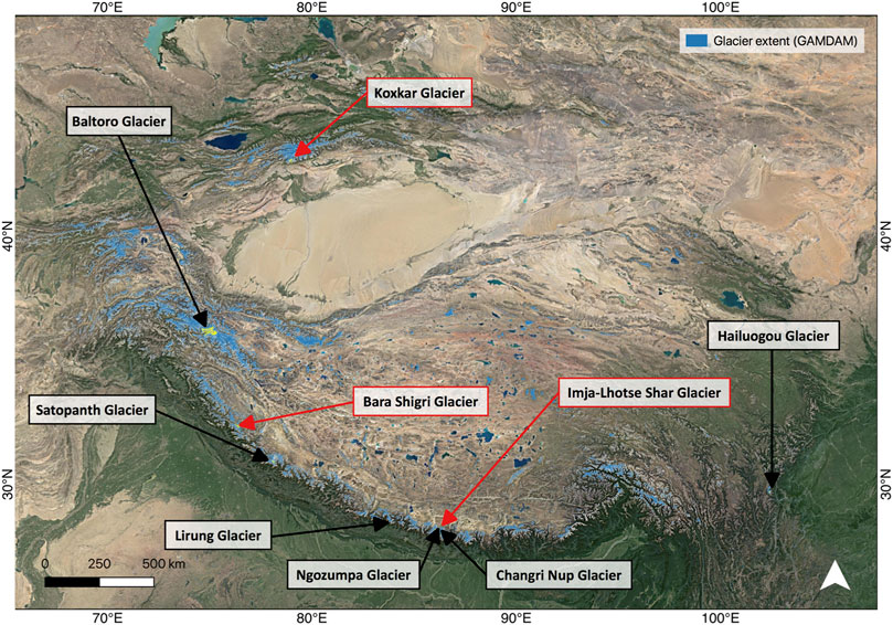
FIGURE 1. The six studied glaciers (black outline and arrow) and the three validation glaciers (red outline and arrow), in the context of the glaciated areas of High Mountain Asia, according to the Glacier Area Mapping for Discharge from the Asian Mountains (GAMDAM) inventory (Sakai, 2019). Base map: Google Satellite Maps.

Deriving Debris Thickness Distribution From Surface Temperature at the Glacier Scale

A systematic comparison of the application of four different forms of the relationship between debris thickness (DT) in cm and surface temperature (T_s) in °C was undertaken. The comparison was carried out on six individual glaciers to determine which form of the equation produces the most accurate debris thickness distribution on each. The four relationships are: linear (Mihalcea et al., 2008a) (Eq. 1), rational curve (McCarthy, 2019) (Eq. 2), an exponential curve from Mihalcea et al. (2008b) (Eq. 3) and an exponential curve from Kraaijenbrink et al. (2017) (Eq. 4).

$DT=c_1{T}_s+c_2(1)$

$DT=\frac{T_s}{c_1+c_2{T}_s}(2)$

$DT=e^{\left(c_1{T}_s-c_2\right)}(3)$

$DT=e^{\frac{\left(T_s-T_{\mathit{s\hspace{0.17em}min}}\right)\text{ln}\left({DT}_{\mathit{max}}\right)}{{\mathit{T}}_{\mathit{s}\hspace{0.17em}95}-T_{s\hspace{0.17em}\mathit{min}}}}(4)$

where c₁ and c₂ are empirically-derived coefficients, T_{s min} is the minimum surface temperature, T_{s 95} is the 95th percentile of surface temperature and DT_max is the assumed maximum debris thickness. The exponential relationships based on Mihalcea et al. (2008b) and Kraaijenbrink et al. (2017) will henceforth be referred to as “exponential (M)” and “exponential (K)”, respectively. The justification for the use of a rational curve to describe the relationship between the surface temperature and debris thickness depends on understanding the components of the surface energy balance model as multiples of either surface temperature or debris thickness. On this basis, the surface energy balance equation for a DCG surface can be rearranged by collecting the surface temperature terms to parameterise debris thickness in the form of a rational curve (Data Sheet S1: Supplementary Note S1).

The in situ debris thickness data were collected from published studies. Data collected using both manual excavation and Ground Penetrating Radar (GPR) were selected to ensure a wide range of debris thicknesses covering large areas of the glaciers. Data collected by manual excavation tended to cover a large proportion of the glaciers’ area with discrete measurements but may have been skewed towards thinner debris, whereas data collected by GPR included thicker debris and tended to cover a smaller proportion of the glaciers’ area but with dense measurements. Only data from the last decade were used, to align approximately with the availability of Landsat 8 thermal imagery (2013-present). Following these criteria, the six datasets selected were from: Baltoro Glacier (Groos et al., 2017), Satopanth Glacier (Shah et al., 2019), Lirung Glacier (McCarthy et al., 2017), Ngozumpa Glacier (Nicholson and Mertes, 2017; Nicholson, 2018), Changri Nup Glacier (Giese, 2019), and Hailuogou Glacier (Zhang et al., 2011) (Figure 2; Supplementary Table S1).

FIGURE 2

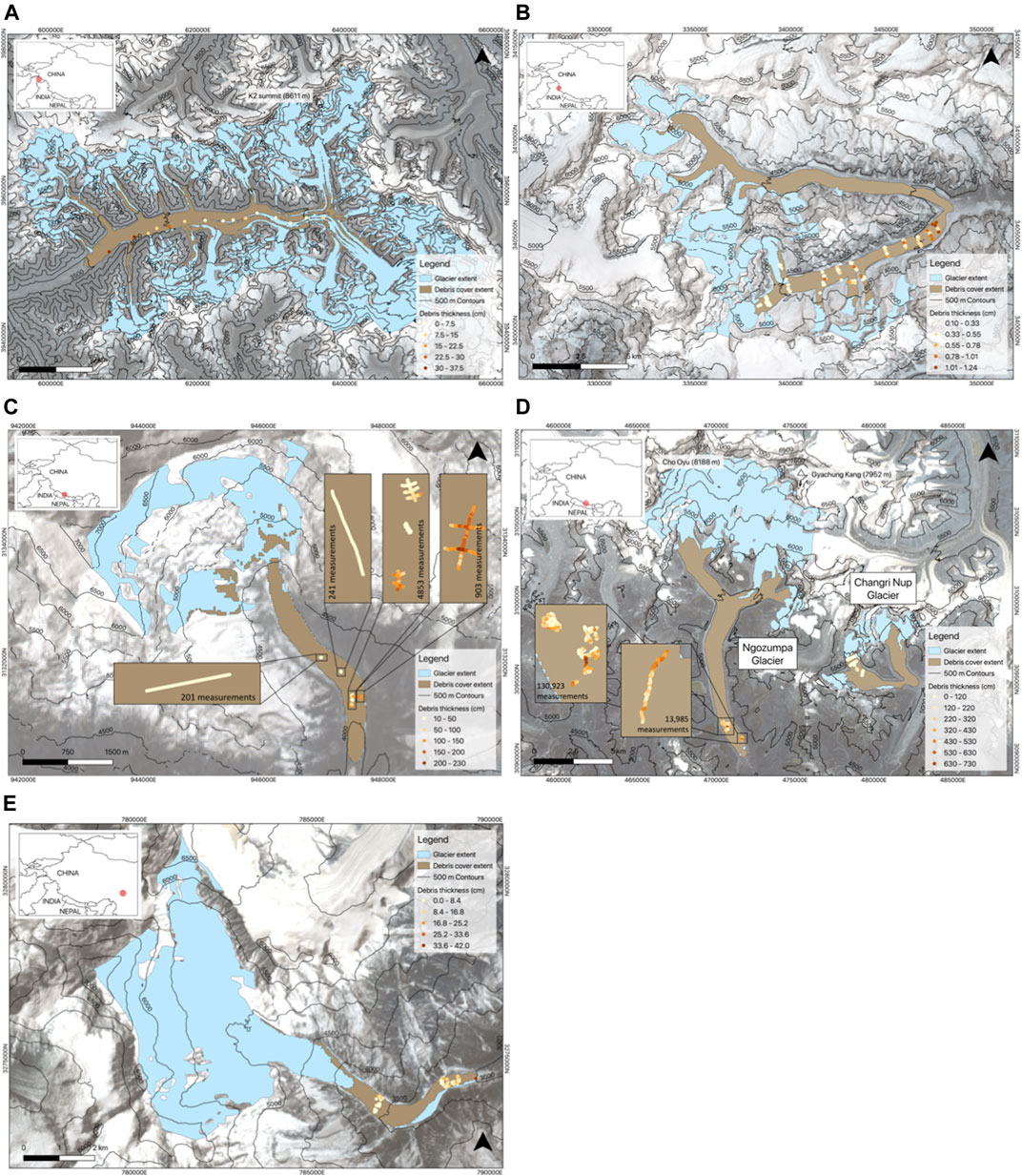
FIGURE 2. Maps to show the distribution of in situ debris thickness measurements for (A) Baltoro (UTM 43N), (B) Satopanth (UTM 44N), (C) Lirung (UTM 45N), (D) Ngozumpa and Changri Nup (UTM 45N), and (E) Hailuogou Glaciers (UTM 47N). Glacier outlines are provided by GAMDAM (Sakai, 2019) and debris cover outlines are provided by Scherler et al. (2018). Note: Giese (2019), consistent with Miles et al. (2018) and Giese et al. (2020), defines the extent of Changri Nup within the southern of the two lobes indicated in this figure and considers the northern lobe to be a separate glacier named Changri Shar. However, for the purposes of this study the outline provided by GAMDAM (Sakai, 2019) is used, which includes both the northern and southern lobe.

The cloud-computing platform, Google Earth Engine (GEE), was used to gather and process satellite thermal band imagery to calculate the land surface temperatures (Figure 3). Landsat 8 data were chosen because they have a sufficiently high temporal and spatial resolution (16-day repeat cycle, acquired at 100 m resolution, but resampled to 30 m in the distributed data products). Landsat 8 has two thermal bands (Band 10 and Band 11), both collected by the Thermal Infrared Sensor (TIRS). Band 10 was chosen because Band 11 has a greater stray light error, resulting in a greater difference between ground-based and TIRS results (Montanaro et al., 2014). A composite thermal image was produced for each glaciated area of interest. The composite image was calculated from multiple thermal images, filtered to account for the variation caused by the variable presence of clouds and shadows, in addition to the seasonal variability of surface temperature itself. The image collection consisted of images with less than 20% cloud cover that fell within the melt season (May–October) in the year the in situ data were acquired, and the 2 years prior. To calculate the composite image from the image collection, the mean Digital Number, excluding the top 20% and bottom 20% of data, was calculated to remove any remaining clouds and shadows that would have exceptionally high or low pixel values, respectively.

FIGURE 3

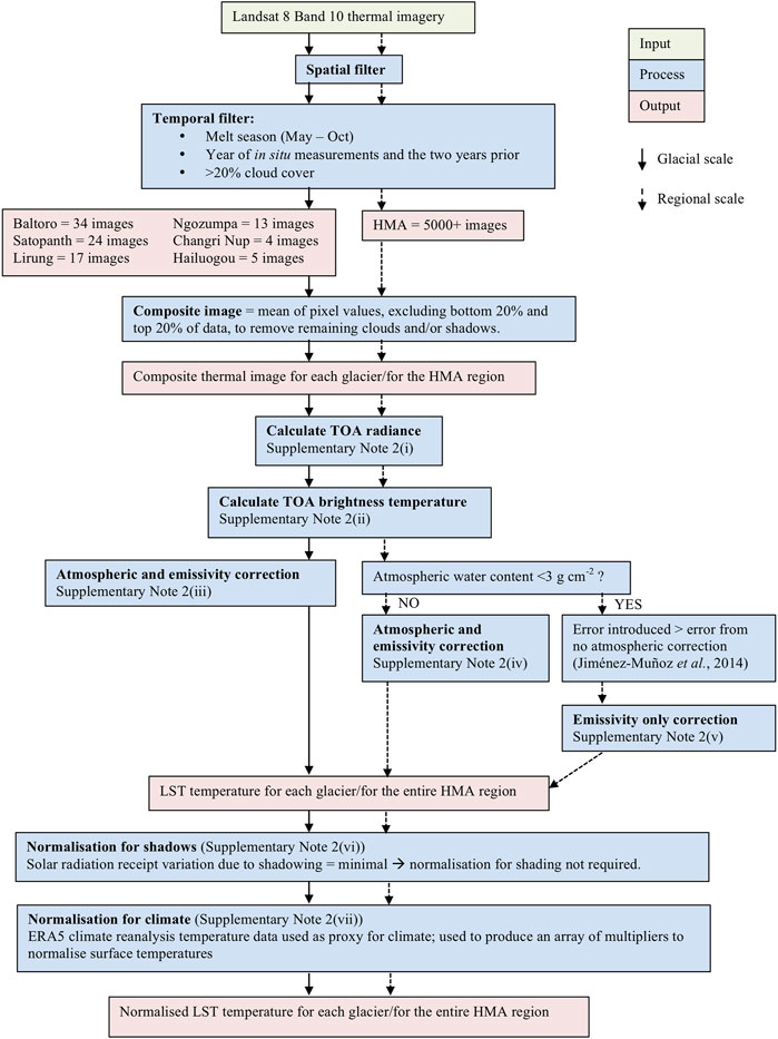
FIGURE 3. Flowchart of methodology to calculate and normalise Land Surface Temperature from Landsat 8 thermal band imagery, within Google Earth Engine.

After calculating the land surface temperature from the composite thermal imagery and correcting it for emissivity and atmospheric effects [Data Sheet S1: Supplementary Note S2(i)–(v)], the data were normalised for climate to account for differences in climate across the HMA region. To do this, a composite image of ERA5 climate reanalysis temperature data was produced for the HMA region, using all data within the melt season (May–October) over the time period in which in situ data were acquired (2013–2016). The average value of the composite image was calculated (287 K), and the percentage difference between the temperature of a pixel according to ERA5 composite and the average value was used to adjust the land surface temperature calculated from the thermal band imagery [Data Sheet S1: Supplementary Note S2(vii)].

Following Mihalcea et al. (2008b) and Kraaijenbrink et al. (2017), this study does not account for temperature change with elevation. The climate normalisation accounts for larger-scale spatial variations in temperature only, not for the changes in temperature with elevation at a glacier scale. Therefore, this should be acknowledged as an inherent limitation with the empirical temperature inversion method. Normalisation for shadows was also considered, but not applied because the effect was considered negligible [Data Sheet S1: Supplementary Note S2(vi)].

The normalised temperature was extracted from the relevant pixel for each debris thickness measurement to form the datasets used to derive the relationships. K-fold cross-validation was used to calculate the error associated with each relationship for each glacier dataset (Brenning et al., 2012). This involves randomly partitioning the dataset into k equal sized subsamples. One subsample is retained to later “test” the relationship, and the remaining subsamples are used as “training” data. The procedure is repeated k times, with each of the subsamples being used once as the “test” set. For our study, we used k = 10.

The median error (ME) and median absolute deviation (MAD) were calculated each time the relationship was trained and the mean of the ten ME values and of the ten MAD values were taken to produce two error values for each relationship. ME is an indicator of accuracy, while MAD is an indicator of precision. Statistics such as the root-mean-square error and the mean error were avoided because they are sensitive to the maximum debris thickness value. This is problematic because the non-linearity of three of the surface temperature/debris thickness equations results in small surface temperature errors having a much greater effect on the derived debris thickness estimates for higher surface temperatures (Evatt et al., 2015; Schauwecker et al., 2015). ME and MAD, however, are insensitive to the maximum debris thickness.

Quantifying the Relationship Between Glaciological Characteristics and Debris Thickness

Terrain characteristics that can influence the distribution of supraglacial debris include elevation, slope, aspect, and curvature (Lawson, 1979; Anderson and Anderson, 2018; Moore, 2018; Nicholson et al., 2018). Each can be extracted from Digital Elevation Models (DEMs). The preferred DEM source was the 8 m HMA DEM produced from high-resolution commercial optical satellite imagery (Shean et al., 2016; Shean et al., 2019). Its coverage is directly dependent on the availability of cloud-free optical imagery but as HMA receives 3,000 mm yr⁻¹ of precipitation, cloud cover is abundant and coverage is discontinuous (Bolch et al., 2012; Yao et al., 2012; Wagnon et al., 2013; Maussion et al., 2014; Salerno et al., 2017). Thus, complete 8 m HMA DEMs were unavailable for Hailuogou Glacier and Baltoro Glacier. For these glaciers, therefore, the 1 arc second (∼30 m) resolution Advanced Spaceborne Thermal Emission and Reflection Radiometer (ASTER) Global Digital Elevation Model Version 3 (GDEM 003) was used for the entire glacier, instead of the 8 m HMA DEM.

For each glacier, elevation values were extracted directly for each grid cell from the respective DEM. Slope, aspect and curvature of each grid cell were extracted using the r.slope.aspect tool in the GRASS QGIS toolbox. This tool compares the pixel value to the values of the adjacent pixels to calculate the slope of each pixel in degrees of inclination from horizontal and the aspect of the slopes in degrees counterclockwise from East. The cosine of aspect was taken subsequently to transform the measurements to a linear scale, from –1 (W) to 1 (E). The tool also calculates the profile curvature of the slope for each pixel, where a negative value represents a concave slope and a positive value represents a convex slope.

Glacier velocity has also been shown to influence the distribution of supraglacial debris (Rowan et al., 2015; Salerno et al., 2017; Bhushan et al., 2018). For each glacier, velocities were extracted from the NASA MEaSUREs ITS_LIVE project (Gardner et al., 2013). They are derived using the autonomous Repeat Image Feature Tracking (auto-RIFT v0.1) processing scheme applied to all Landsat 7 and 8 images acquired between August 2013 and May 2016 with 80% cloud cover or less (Gardner et al., 2018). Image pairs are searched for matching features, as defined by Normalised Cross Correlation maxima (Paragios et al., 2006). Both the terrain and velocity datasets were resampled to the grid size of the derived debris thickness datasets.

To determine statistically the relationship between debris thickness and these glaciological characteristics, two statistical tests were carried out on the dataset for each glacier. First, the non-parametric Spearman’s Rank Correlation Coefficient was calculated by correlating all the derived debris thickness pixel values with each glaciological characteristic (elevation, slope, aspect, curvature, and velocity) for the corresponding pixel, for each individual glacier. A non-parametric test was chosen because none of the individual datasets were normally distributed, as determined using the Kolmogorov–Smirnov test with 99% confidence. However, it should be noted that this technique does not account for spatial autocorrelation. Furthermore, the correlation coefficients between debris thickness and each of the five glaciological variables ignore the role of any correlations between the glaciological characteristics. This covariance is high in some cases (Supplementary Table S2), which reduces the reliability of some of the correlation coefficients. Principal Components Analysis (PCA) diagnoses correlations among the glaciological characteristics by detecting patterns of variability that are shared between them. Second, therefore, for each glacier an unrotated PCA was carried out on datasets consisting of only the elevation, slope, aspect, curvature, and velocity data. Principal Components (PCs) were found, which are linear combinations of the glaciological characteristics that explain the directions of maximum variance in each glacier’s dataset. The debris thickness data were excluded from the PCA because the glaciological characteristics describing the terrain and velocity of each glacier were treated as a priori controls on the spatial distribution of supraglacial debris thickness. The debris thickness data were later regressed against the PCs with an eigenvalue greater than or equal to 1, using forward stepwise regression. The regression equations were used to assess how much of the debris thickness variability could be explained by these PCs, in addition to the strength and direction of the contribution of each PC to debris thickness variability, for each glacier.

Deriving Debris Thickness Distribution at the Regional Scale

Debris thickness and surface temperature data from the six individual glaciers were collated and the four forms of empirical relationship (linear, rational, exponential (M), and exponential (K) were fitted to the combined dataset. Errors (ME and MAD) were calculated based on the results of a k-fold cross validation. The relationship with the smallest error was used to calculate debris thickness distribution from surface temperature over the entire HMA region.

The land surface temperature of the entire region was calculated from a composite thermal image produced for the HMA region in largely the same way as described for each glaciated area of interest (see Section Deriving Debris Thickness Distribution From Surface Temperature at the Glacier Scale). The only difference is the correction for the emissivity and atmospheric effects (Figure 3). The single-channel atmospheric correction algorithm implemented at the glacier scale [Data Sheet S1: Supplementary Note S2(iii)] could not be used at a regional scale because the parameter values vary significantly over space. The variation of these parameters can be approximated by water vapour [Data Sheet S1: Supplementary Note S2(iv)]. However, the atmospheric water content of the region is <3 g cm⁻², which introduces error greater than if no atmospheric correction was performed (Jiménez-Muńoz et al., 2014). Thus, an emissivity-only correction was performed [Data Sheet S1: Supplementary Note S2(v)]. The coverage of the composite thermal image was continuous over the entire HMA region due to the vast amount of Landsat imagery available over the region within the specified time period.

Results

Derivation of Debris Thickness at the Glacier Scale

Five of the six glacier debris thickness/surface temperature datasets show a positive correlation, while Lirung Glacier shows a negative correlation (Table 1). On closer inspection, the data for Lirung Glacier seem to comprise two samples, one of relatively high debris thickness values for low surface temperatures and one of relatively low thickness values for high temperatures. The two samples come from different parts of the glacier; the high thickness/low temperature group from close to the eastern margin and the low thickness/high temperature set from the central flowline and towards the western margin (Figure 2C). This could be a result of shading patterns, the presence of snow or interstitial ice or the unintentional bias of where debris thickness measurements were taken within the larger 30 m grids. We further note that the debris thickness measurements covered a relatively small area of the glacier compared to those on the other glaciers (the high temperature set represents just five 30 m pixels). Furthermore, the range of temperatures sampled is small (between 18 and 25°C) by comparison with the range measured across the whole glacier (0 and 29°C), whereas the range sampled on the other glaciers is more representative of their full range. For these reasons, the Lirung Glacier data set is excluded from further analysis at the glacier scale. The four forms of empirical relationship fitted to the data from the remaining five glaciers are shown in Figure 4 and the derived constants for the relationships are given in Table 2.

TABLE 1

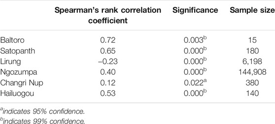
TABLE 1. Correlations between the debris thickness/surface temperature datasets, for each glacier.

FIGURE 4

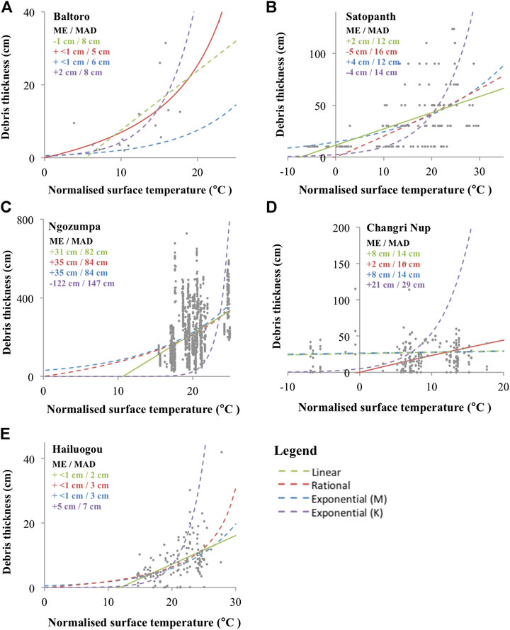
FIGURE 4. Comparison of the errors of the linear (green), rational curve (red), exponential (M) (blue), and exponential (K) (purple) forms of the relationship between debris thickness and surface temperature for (A) Baltoro Glacier, (B) Satopanth Glacier, (C) Ngozumpa Glacier, (D) Changri Nup Glacier, and (E) Hailuogou Glacier. Circles represent data points, solid line indicates chosen relationship, dashed lines represent remaining relationships.

TABLE 2

TABLE 2. Constants derived for each of the four forms of debris thickness/surface temperature relationship [linear, rational curve, exponential (M) and exponential (K)], for all six glaciers and for the HMA region.

For the five glaciers, the “best” relationship was taken to be that with the smallest ME (highest accuracy); for Baltoro and Hailuogou Glaciers, where two relationships had similarly high accuracies, the relationship with additionally the smallest MAD (highest precision) was chosen (Figure 4). Different forms of relationship perform best across the five glaciers. The linear relationship performs best for three (Satopanth, Ngozumpa and Hailuogou Glaciers) and the rational curve performs best for two (Baltoro and Changri Nup Glaciers). For each glacier, the best relationship was used to derive the debris thickness distribution across its entire surface from the surface temperature measurements (Figure 5).

FIGURE 5

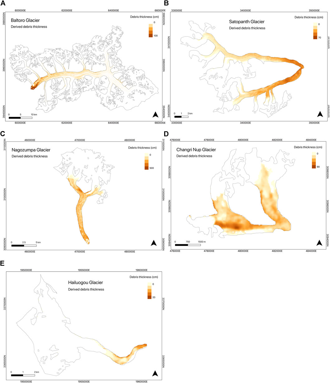
FIGURE 5. Derived debris thickness distributions for the debris-covered parts of (A) Baltoro Glacier, (B) Satopanth Glacier, (C) Ngozumpa Glacier, (D) Changri Nup Glacier, and (E) Hailuogou Glacier. Glacier outlines are provided by GAMDAM (Sakai, 2019). See note in caption for Figure 2 regarding Changri Nup Glacier outline. Note that debris thickness scales vary between glaciers.

In addition to the ME and MAD values of the debris thickness relationships, the descriptive statistics of the modeled and measured debris thickness values are compared to further assess their error (Table 3). The modeled mean and median debris thicknesses generally correspond well to their respective measured values, particularly for Baltoro, Satopanth, Changri Nup, and Hailuogou Glaciers where the modeled and measured mean debris thicknesses vary by less than ∼7 cm and the median values vary by less than ∼10 cm. The difference between the modeled and the measured mean debris thicknesses is understandably greater for Ngozumpa Glacier at ∼50 cm, where the ME of the surface temperature/debris thickness relationship is greater. However, the modeled and the measured median debris thicknesses correspond well for Ngozumpa Glacier. With respect to the standard deviation of the modeled and measured debris thicknesses, the values generally correspond well, particularly for Baltoro, Satopanth, Changri Nup, and Hailuogou Glaciers, but less so for Ngozumpa Glacier where the modeled standard deviation is significantly less than the measured. This is most likely a result of the model being less able to replicate the thick debris on Ngozumpa Glacier given the relationship between surface temperature and debris thickness decays with increasing debris thickness (Taschner and Ranzi, 2002).

TABLE 3

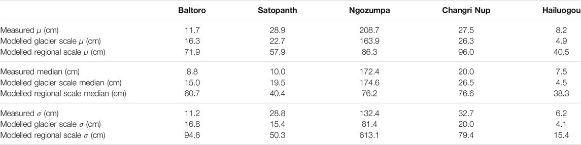
TABLE 3. Comparison of the measured and modeled mean (µ), median and standard deviation (σ) debris thicknesses, at a glacier scale and at a regional scale.

Overall, we have confidence that the derived debris thickness maps are realistic, albeit with a centimetre to decimetre scale error. The debris thickness distributions for the five glaciers are used for further analysis to assess the controls on the spatial distribution of debris cover.

Quantification of the Relationship Between Glaciological Characteristics and Debris Thickness

The Spearman’s Rank Correlation Coefficients between debris thickness and the glaciological characteristics are shown in Table 4. The strongest and most consistent correlation is the negative relationship between debris thickness and elevation, showing that thicker debris occurs at lower elevations. There is also a consistent negative relationship between debris thickness and velocity, suggesting that debris thickens as velocity decreases. There is a weak positive relationship between debris thickness and slope for all of the glaciers, except Baltoro. The relationship between debris thickness and aspect is mixed in both strength and direction, and the relationship with curvature is weak in most cases.

TABLE 4

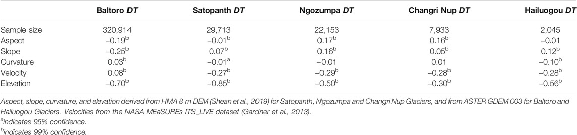
TABLE 4. Correlations between debris thicknesses derived at a glacier scale and selected glaciological characteristics (aspect, slope, curvature, velocity, and elevation).

The component loadings of each PC (i.e., the correlation of each PC with a given glaciological characteristic) with an eigenvalue equal to or greater than 1 are given in Table 5, alongside the regression of debris thickness (DT) with these PCs, for each glacier. In most cases, elevation and velocity have the largest component loadings in PC1. All the regression relationships have the strongest relationship between debris thickness and PC1. This suggests that a proportion of the variation in debris thickness (as determined by the R² value) is principally controlled by elevation and velocity. The negative value of the relationship suggests that thicker debris is more likely on ice at low elevations with slower velocities. Baltoro Glacier is an exception to this as the largest component loadings in PC1 are the large positive values for slope and elevation, and the large negative value for velocity. The negative value of the relationship between debris thickness and PC1 on Baltoro suggests that thicker debris is more likely on ice with flatter slopes at lower elevations but with higher velocities, although the proportion of debris thickness variation explained by the PCs is very low (R² = 0.010).

TABLE 5

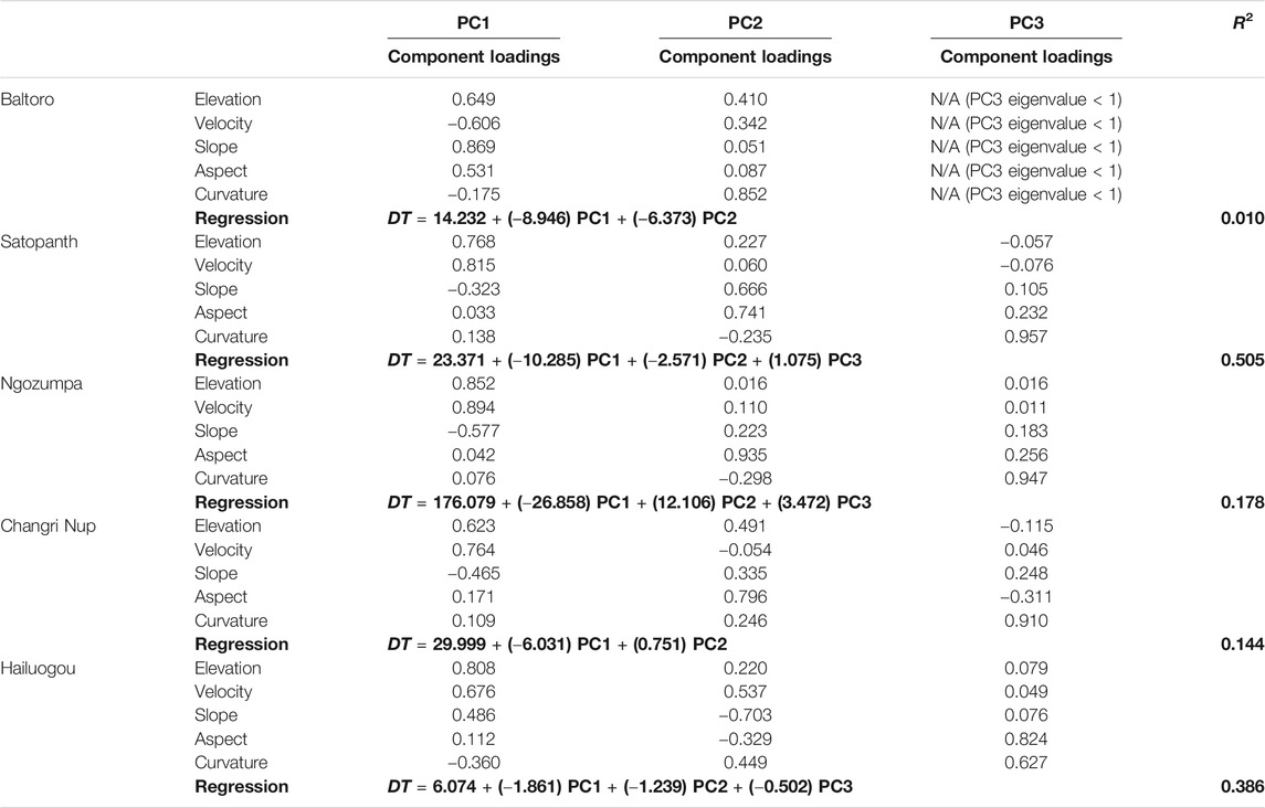
TABLE 5. Component loadings of the Principal Components (PCs) with an eigenvalue equal to or greater than 1, and the regression equations and R² values (bold) of debris thickness (DT) with PCs as independent variables, for each glacier.

The greatest component loadings in PC2 are slope and aspect in most cases, except for Baltoro and Hailuogou Glaciers. The relationship with PC2 is not consistent between the glaciers. Where PC2 has large, positive component loadings for slope and aspect, the relationship between PC2 and debris thickness is positive for Ngozumpa and Changri Nup, but negative for Satopanth. Therefore, on Satopanth, thicker debris is more likely on flatter, west-facing slopes, but on Ngozumpa and Changri Nup, thicker debris is more likely on steeper, east-facing slopes. Where PC2 has a large, positive component loading for curvature (Baltoro Glacier), the relationship with debris thickness is negative, suggesting that on this glacier, thicker debris is more likely on concave slopes.

The role of curvature also presides in the inclusion of PC3 in the regression relationships for Satopanth, Ngozumpa, and Hailuogou Glaciers. This suggests that thick debris is more likely on convex slopes on Satopanth and Ngozumpa Glaciers, but on concave slopes on Hailuogou Glacier. However, the contribution of curvature is not as dominant as the contribution of elevation, velocity, slope and aspect on these glaciers.

This analysis has quantified the interplay between five glaciological characteristics across five glaciers, highlighting dominant relationships between velocity and elevation, and between slope and aspect. Furthermore, it has quantified the ways in which the interaction of the characteristics explains a proportion of the variability in debris thickness across the five glaciers. In all cases, the relationship between debris thickness and PC1 is stronger than the relationship between debris thickness and PC2, suggesting that the contribution of velocity and elevation to debris thickness variability dominates over the contribution of slope and aspect for all the studied glaciers, except Baltoro where slope dominates. Moreover, this analysis reveals the small contribution of curvature on the distribution of debris thickness on four of the five glaciers.

Map of Debris Thickness Distribution at the Regional Scale

To calculate the pattern of debris thickness distribution across the entire HMA, it is important to use a robust empirical relation that has been derived using data from a wide range of climate and topographical settings. The combined surface temperature/debris thickness dataset from the six glaciers has a mean debris thickness of 2.02 m, a median of 1.64 m, a standard deviation of 1.33 m, and a range spanning 0–7.34 m. This would appear to be representative of the debris thickness distribution we might expect on DCGs in the HMA region (Nicholson and Benn, 2013; Juen et al., 2014; Rounce and McKinney, 2014; Rounce et al., 2015). For the collated dataset (n = 151,821), the non-parametric Spearman’s Rank Correlation Coefficient between surface temperature and debris thickness was 0.30 (99% confidence). The linear, rational curve, exponential (M) and exponential (K) relationships were fitted to this collated dataset and are graphed in Figure 6, with the derived constants given in Table 2. The Lirung Glacier data were included in this work because the possible sampling bias that was apparent at the glacier scale (Figure 2) was not apparent in the context of the entire dataset for all six glaciers (Figure 6).

FIGURE 6

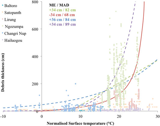
FIGURE 6. Comparison of the errors of the linear relationship (green), rational curve (red), exponential (M) (blue), and exponential (K) (purple) forms of the relationship between debris thickness and surface temperature for the collated dataset from all six glaciers. The solid line indicates the chosen form of the relationship.

The accuracies are the same for the linear relationship, the rational curve and the exponential (K) relationship, but the debris thickness is underestimated with the rational curve (ME = −34 cm) and overestimated with the linear and exponential (K) relationships (MEs = +34 cm). The rational curve has a smaller MAD (68 cm) than that for the linear and exponential (K) relationships (82 and 89 cm respectively) and is therefore the most precise. Although the MAD remains high for the rational curve, it is the best available with the given data for deriving debris thickness from surface temperature at the regional scale. We apply this relationship within the GEE platform to the debris-covered glaciated areas of the HMA region. The GEE code is available in the Data Sheets S2, S3.

Comparison of the debris thickness modeled using the regional scale relationship with the in situ debris thickness measurements available for the five glaciers analyzed above reveals that the regional scale relationship overestimates the mean and median debris thickness for glaciers with a relatively thin debris cover (Baltoro, Satopanth, Changri Nup, and Hailuogou Glaciers), but underestimates the mean and median debris thickness for glaciers with a relatively thick debris cover (Ngozumpa Glacier) (Table 3).

Due to the lack of in situ debris thickness data on other HMA glaciers, the accuracy of the relationship applied to other glaciers cannot be quantified. Thus, the method is validated by comparing qualitatively the debris thickness distributions produced by this relationship to maps of debris thickness produced using other remote sensing methods in the literature: Koxkar Glacier, Central Tien Shan (Juen et al., 2014); Imja-Lhotse Shar Glacier, Nepal Himalaya (Rounce and McKinney, 2014); and Bara Shigri Glacier, Indian Himalaya (Schauwecker et al., 2015). Their locations are in Figure 1 and their debris thickness distributions are in Figure 7.

FIGURE 7

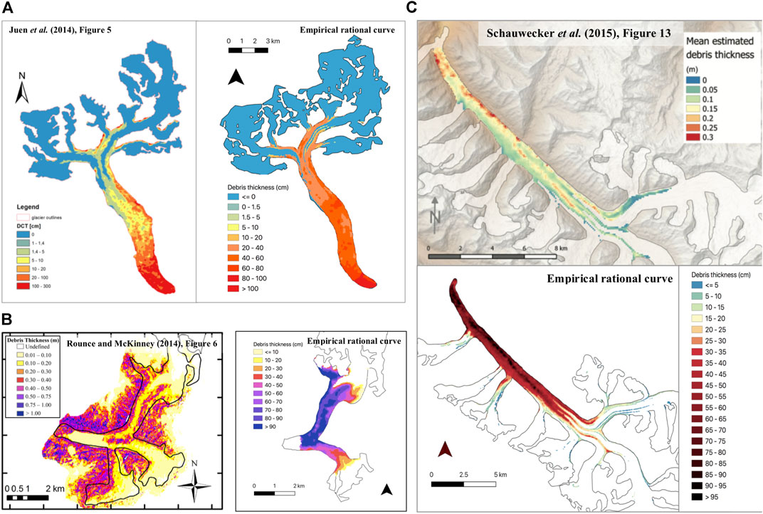
FIGURE 7. Derived debris thickness distributions for the debris-covered parts of (A) Koxkar Glacier (UTM 44N), (B) Imja-Lhotse Shar Glacier (UTM 45N), and (C) Bara Shigri Glacier (UTM 44N), in comparison to published maps of derived debris thickness.

The debris thickness distribution on Koxkar Glacier produced using our method is very similar to that produced by Juen et al. (2014) (Figure 7A). In both cases, the debris is thicker closer to the terminus and along the eastern margin, and thinner upglacier. However, compared to the distribution produced by Juen et al. (2014), our distribution overestimates the thin debris upglacier by up to 30 cm and underestimates the thick debris near the terminus by up to 150 cm in some places. According to both our method and Rounce and McKinney (2014), on Imja-Lhotse Shar, thicker debris is present on the northern limb, particularly on the western margin and along the central flowline, while thinner debris dominates on the southern limb. On both limbs, the debris thins upglacier according to both methods (Figure 7B). Similarly, on Bara Shigri, both our method and Schauwecker et al. (2015) show the debris is thickest at the terminus and along the north-eastern margin and thins upglacier (Figure 7C). For both Imja-Lhotse Shar and Bara Shigri, however, our method tends to overestimate debris thickness by up to 50 cm for Imja-Lhotse Shar and by up to 60 cm for Bara Shigri. Both Rounce and McKinney (2014) and Schauwecker et al. (2015) comment that their methods tend to underestimate debris thickness but do not state by how much. Their underestimation would at least partly explain the differences between their modeled debris thickness values and those produced by our method.

Overall, the regional relationship performs well with regards to replicating the values and patterns of debris across all eight glaciers compared, but the depth of thin debris cover tends to be overestimated while that of thick debris cover tends to be underestimated. This is an expected result given the large ME and MAD (−34 and 68 cm, respectively) in comparison to the mean debris thickness of the region (2.02 m). Furthermore, there is a lack of independent in situ debris thickness data with which to validate these results. Therefore, although the patterns of debris thickness distribution determined by alternative methods are qualitatively replicated using the regional application of this empirical rational curve, its performance cannot be validated quantitatively. Thus, despite this empirical relationship improving upon the precision of the empirical relationship of Kraaijenbrink et al. (2017), the results should be treated with caution.

Discussion

Debris Thickness at the Glacier Scale

For five out of the six glaciers, the derived surface temperature/debris thickness relationship produced glacier-scale debris thickness distributions with centimetre to decimetre scale errors. A rational curve was the most accurate for Baltoro and Changri Nup Glaciers, while a linear relationship was best for Satopanth, Ngozumpa and Hailuogou Glaciers. Over the range of input data, these two relationships perform similarly (Figure 4). The exponential (K) relationship consistently performs the worst and can be explained by the extent to which it responds to input data. The linear and rational curves are extrapolation approaches (Mihalcea et al., 2008a), whereas the exponential (K) relationship is a scaling approach (Kraaijenbrink et al., 2017). The extrapolation approaches use all input data to calculate parameters, whereas the scaling approach scales the relationship between 1 cm (assumed to be at the minimum surface temperature) and the maximum debris thickness (assumed to be at the 95th percentile of surface temperature). Thus, the extrapolation approaches are likely to produce more accurate debris thickness distributions because they are optimised using the entire dataset, whereas the scaling approach is optimised using only two data points.

For the extrapolation approaches to prove successful, the input data must be well distributed and represent the full range of debris thicknesses and surface temperatures across the glacier. This was why a realistic debris thickness/surface temperature relationship could not be derived for Lirung Glacier because its input surface temperature range was only 18–25°C, but the surface temperature of the debris-covered area reached 0°C upglacier. This represents a limitation with the distribution of the in situ dataset, which was focused near the glacier terminus and did not reflect the full range of surface temperatures present.

The success of the rational curve in producing the most accurate debris thickness distributions for Baltoro and Changri Nup Glaciers is important because the only non-linear relationships applied previously in published works have been exponential forms (Mihalcea et al., 2008b; Kraaijenbrink et al., 2017). The success of the rational curve could be because it passes through the origin and so calculates clean ice to be at 0°C. The surface temperature datasets used to derive the relationships are mean values over the melt seasons, so clean ice can be assumed to be at its melting point of 0°C. Therefore, the rational curve provides a physically accurate representation of the surface temperature/debris thickness relationship. However, the rational curve does not perform best for all glaciers. It is not clear which factors, if any, cause the linear relationship to perform better. Tentatively, we suggest that debris thickness may influence whether the linear relationship or rational curve provides a better fit to the data. Satopanth and Ngozumpa Glaciers, where a linear relationship is more accurate, have thicker debris covers than Baltoro and Changri Nup, where a rational curve is more accurate. The distribution of debris thickness data used to fit the relationship is also likely a controlling factor, in addition to the potential role of glacier-specific debris sources. Due to the limited number of glaciers studied, these suggestions are only tentative, and more research is required in this regard.

The Relationship Between Glaciological Characteristics and Debris Thickness

The percentage of debris thickness variability explained by the PCs varies between 1% for Baltoro Glacier and 50% for Satopanth Glacier. The PCs represent the combined influence of surface elevation, slope, aspect, curvature and velocity. Elevation and velocity represent primary controls on debris dispersal. Elevation is a proxy for mass movement, by representing the cumulative effects of mass movement processes from the valley sides (Dunning et al., 2015), and for ablation rate, which partially controls melt out rate of englacial debris (Rowan et al., 2015). Velocity represents the influence of ice flow on the concentration of debris through horizontal compression. Slope, aspect and curvature are surrogates for factors controlling the secondary mechanisms of debris dispersal. However, mass movement processes from the valley sides and the melt out of englacial debris cannot be explained by elevation alone. Therefore, it is possible that the unexplained debris thickness variance is explained by processes related to mass movement from the valley sides or the melt out of englacial debris, but which are not fully accounted for in the PCs, such as bedrock geology.

Of particular note is the minimal proportion of debris thickness variability explained on Baltoro Glacier, where just 1% is accounted for by the PCs. Figure 2A highlights the presence of multiple tributary glaciers feeding Baltoro Glacier. Thus, the emergence of englacial debris at the confluence of multiple ice sources is likely to be a dominant mechanism controlling the distribution of debris thickness here (Eyles and Rogerson, 1978; Deline, 2005). This mechanism is not accounted for in the selected glaciological characteristics and provides a potential explanation as to why only 1% of the debris thickness variability is explained. Given the negligible proportion of debris thickness variability explained, the relationship between glaciological characteristics and debris thickness on Baltoro Glacier is not discussed further.

On Satopanth, Ngozumpa, Changri Nup, and Hailuogou Glaciers, results show that thicker debris is more likely to be found where elevation and velocity are both low (Table 5). This is an expected finding given previous observations that debris thickness tends to increase towards the terminus (Kirkbride and Warren, 1999; Anderson, 2000; Kellerer-Pirklbauer, 2008; Mihalcea et al., 2008b; Gibson et al., 2017), where ice is lower lying and slower moving (Kirkbride, 2002; Quincey et al., 2009a; Quincey et al., 2009b; Scherler et al., 2011b). Lower elevations, and therefore warmer temperatures, initially encourage the melt out of englacial debris (Kirkbride and Deline, 2013) and encourage erosion (Heimsath and McGlynn, 2008; Banerjee and Wani, 2018). Once enough debris cover has built up to inhibit ablation, the zone of maximum velocity shifts upglacier due to the decreasing thickness and slope of the debris-covered portion, resulting in a slow-flowing debris-covered tongue (Scherler et al., 2011a). The negative velocity gradient causes debris thickness to increase further due to horizontal compression, as dictated by the law of mass conservation (Nakawo et al., 1986; Anderson and Anderson, 2016).

On Satopanth Glacier, the results indicate that thicker debris is found on flatter, west-facing slopes. This relationship agrees with the literature, which states that thicker debris is more likely on flatter slopes, where the chance of debris sliding is lower (Moore et al., 2018; Nicholson et al., 2018). The incidence of sliding is also reduced on slopes with a lower receipt of solar radiation, i.e., northwest-facing slopes in the Northern Hemisphere (Hock and Noetzli, 1997), because meltwater production is lower and therefore less able to act as a lubricant for sliding. Thus, debris is more likely to build up to greater thicknesses where meltwater production is less (Lawson, 1979; Nicholson et al., 2018). Satopanth Glacier is the only glacier to corroborate previous findings in the literature with regards to the way in which velocity/elevation and slope/aspect control debris thickness distribution.

On the remaining glaciers (Hailuogou, Ngozumpa, and Changri Nup), debris thickness variability is principally controlled by velocity and elevation (PC1) in the same way as on Satopanth Glacier. However, for these three glaciers, slope and aspect have unexpected relationships with debris thickness. On Hailuogou Glacier, thicker debris is more likely to be found on steeper slopes and on Ngozumpa and Changri Nup Glaciers thicker debris is more likely on steeper, east-facing slopes. This contrasts to the literature, which states sliding is more likely to occur on steeper, east-facing slopes (Lawson, 1979; Moore et al., 2018; Nicholson et al., 2018), causing thinner debris to dominate in these locations.

It is possible that a methodological bias caused this unexpected relationship. The Landsat satellite has a sun-synchronous orbit and so the images used to derive debris thicknesses were taken at 10:11 (±15 min) Mean Local Time (MLT). At the time the images are taken, the sun azimuth varies between 120° and 140° and so the southeast-facing slopes receive the most direct sunlight. This could result in a bias towards greater surface temperatures, and therefore calculated thicker debris, on southeast-facing slopes. Furthermore, the sun elevation angle, at the time the images are taken, varies between 55° and 65°. Thus, slopes at this angle would receive the sunlight most directly, compared to flatter slopes where the sunlight would be spread over a larger area. The slopes on the debris-covered surfaces have a maximum of 70°. Thus, the steeper slopes could be biased towards higher surface temperatures, and towards calculated thicker debris. Therefore, the occurrence of thicker debris on steeper, southeast-facing slopes on Hailuogou, Ngozumpa, and Changri Nup Glaciers could be due to this methodological bias.

However, because the thermal images used to calculate the land surface temperature are all acquired at the same time of day and the temperatures were normalised to take into account spatial variations in the climate of the region, this methodological bias would occur systematically, such that all steep and southeast-facing slopes would be affected. Such a bias does not seem to occur on Satopanth Glacier, where thicker debris occurs on flatter, west-facing slopes. Furthermore, when looking at the regional scale debris thickness distribution, there does not appear to be widespread evidence that glaciers with a predominantly easterly aspect have thicker debris cover than glaciers with different aspects. If the outlined bias had a notable impact, it would likely be evident on all debris thickness distributions, but it does not appear to be, so the likelihood of a methodological bias is small.

Therefore, it is suggested that the debris is, in fact, thicker on steep, east-facing slopes on Ngozumpa, Changri Nup, and Hailuogou Glaciers. However, local scale slope and aspect are not necessarily the factors controlling the prevalence of thick debris. Isolated areas of thick debris cover may result from the occurrence of localised supraglacial debris supply from mass movement from the valley sides (Dunning et al., 2015). On Ngozumpa, Changri Nup, and Hailuogou Glaciers, isolated patches of thick debris can be identified. On the southern of the two lobes comprising Changri Nup Glacier, there is a thick ridge of debris in the glacier’s midline (Figure 5D). The debris that emerges as part of this surface ridge is eroded from a large rocky spur that generates many rockfalls (Giese, 2019). On Ngozumpa Glacier, there is an isolated area of thick debris cover near the upglacier limit of debris cover, on the northern edge of the northwestern branch (Figure 5C). On Hailuogou Glacier, thick debris can be identified along the entire northern edge of the debris-covered tongue (Figure 5E). It is possible that these areas of thick debris cover on Ngozumpa and Hailuogou Glaciers are also caused by mass movement onto the glacier surface, rather than by the gravitational reworking of debris as a result of the local slope and aspect of the surface. Images in Data Sheet S1: Supplementary Note S3 show scars on the valley sides suggesting large scale mass movement onto these specific areas of Ngozumpa and Hailuogou Glaciers.

The role of valley side mass movement has not been comprehensively considered in this study; only implicitly with elevation as a proxy. To do so would involve consideration of the valley side slopes (Scherler et al., 2011b), temperatures (Nagai et al., 2013; Banerjee and Wani, 2018; Kuschel et al., 2020) and geologies (Fischer et al., 2012), all of which control the temporal and spatial occurrence of mass movement processes (Draebing and Krautblatter, 2019). The images in Data Sheet S1: Supplementary Note S3 take the first steps required to investigate whether the unexpected relationships between debris thickness and slope/aspect on Ngozumpa, Changri Nup, and Hailuogou Glaciers are caused by large scale mass movement processes rather than local scale debris transfer processes, but further research is needed.

The results on Satopanth, Ngozumpa and Hailuogou Glaciers are of particular interest because the regression relationships suggest a relationship between curvature and the distribution of debris thickness. The role of curvature is less than that of velocity/elevation and slope/aspect, but to the authors’ knowledge these are the first empirical relationships to have been found between curvature and debris thickness (cf. Nicholson et al., 2018). On Hailuogou Glacier, the debris is thicker where slopes have a concave profile. This agrees with the expectation that debris should become more stable in a downslope direction on concave slopes as the gradient of the slope decreases (Moore, 2018). However, on Satopanth and Ngozumpa Glaciers, the debris is thicker on slopes with a convex profile. The reasons for this are currently unknown and require further research.

Debris Thickness Distribution at the Regional Scale

To the authors’ knowledge, Kraaijenbrink et al. (2017) have produced the only published estimate of glacier debris thickness distribution for the entire HMA region. However, the present study suggests that a rational curve is equally, if not more, appropriate for deriving debris thickness from surface temperature over the HMA region. The ME of the rational curve (−34 cm) is equal in magnitude to the ME of the exponential (K) relationship (+34 cm), but the exponential (K) overestimates debris thickness, while the rational curve underestimates it. The MAD associated with the rational curve (68 cm) is smaller than that associated with the exponential (K) curve (89 cm). Therefore, the use of the rational curve rather than the exponential (K) curve has the potential to derive more precise glacier debris thickness distributions across HMA. Despite this improved precision, the results should be treated with caution given the ME and MAD remain high as a proportion of the mean debris thickness of 2.02 m, at 17 and 34%, respectively.

Figure 8 displays the difference between the debris thickness derived using the rational curve and that derived using the exponential (K) relationship. The greatest difference between the two distributions occurs at the glacier termini, where debris is thickest. The exponential (K) relationship calculates debris to be >3 m thicker than that calculated by the rational curve in some cases. However, for areas with thinner debris covers, such as upglacier locations, the two relationships produce comparable results. This is because the relationships are very similar until ∼10°C (∼30 cm), at which point the rational curve begins to underestimate debris thickness and the exponential (K) relationship begins to overestimate debris thickness for a given surface temperature (Figure 6).

FIGURE 8

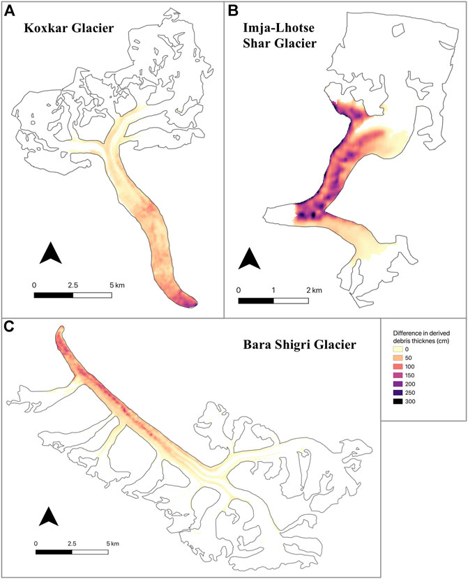
FIGURE 8. The difference between the debris thickness calculated using rational curve and the exponential (K) form of the regional scale empirical relationship, for (A) Koxkar Glacier, (B) Imja-Lhotse Shar Glacier, and (C) Bara Shigri Glacier (difference calculated by subtracting rational curve debris thickness from exponential (K) debris thickness).

The application of either empirical relationship to the entire HMA region is inevitably associated with some limitations, primarily as a result of the large spatial variations in temperature that exist in the HMA region (Bookhagen and Burbank, 2010; Bolch et al., 2012; Kapnick et al., 2014; Rounce et al., 2019). However, the impact of this limitation has been mitigated in this study, namely though the climate normalisation applied to the thermal imagery [Data Sheet S1: Supplementary Note S2(vii)]. Furthermore, there is seasonal variability in land surface temperature. The use of composite thermal images calculated from the mean of thermal imagery over the melt season addresses this issue (Figure 3). The reduction of climatic influence and seasonal variation in this way increases the proportion of surface temperature controlled by debris thickness, and thus increases our confidence in the regional application of the relationship.

Limitations

There are several limitations of our approach to calculating glacier debris thickness. First, calculating land surface temperature from thermal satellite imagery inevitably means that the calculated temperature represents at best a 30 m × 30 m area (resampled from a 100 m × 100 m area). Only a single debris thickness value can be derived for a pixel area represented by a single surface temperature value. However, debris thickness varies on a scale smaller than a 30 m × 30 m area (Nicholson and Benn, 2013). In the datasets used to derive the empirical relationships, there is often a range of debris thickness measurements associated with a single surface temperature (Figure 4). The details of this heterogeneity are not displayed in the derived debris thickness distributions, although it does contribute to our error calculations. Thus, there is a need for future research to quantify debris thickness variability within a 30 m × 30 m area. The acquisition of more detailed in situ datasets would contribute towards this and allow for statistical modeling (e.g., the construction of semi-variograms) or interpolation (e.g., kriging) at finer spatial scales than the resolution of the thermal imagery.

Second, the empirical relationship between surface temperature and debris thickness is less accurate at greater debris thicknesses. This is because as debris thickness increases, the influence of glacier ice on the surface temperature decreases, and eventually stops, due to the reduced effectiveness of heat conduction with depth (Taschner and Ranzi, 2002; Ranzi et al., 2004). Thus, a warmer surface temperature may represent a wider range of debris thicknesses than a cooler surface temperature. This exposes another limitation of this empirical method in that it performs best for thinner debris, where the relationship between surface temperature and debris thickness is stronger (Mihalcea et al., 2006; Mihalcea et al., 2008a; Mihalcea et al., 2008b). However, melt rates below a thick debris layer are generally low, and so the impact of this limitation will be negligable in the context of a melt model.

Third, the temperature inversion method does not account for variation in surface temperature with elevation. Following the work of Mihalcea et al. (2008b) and Kraaijenbrink et al. (2017), surface temperature is assumed to vary solely in response to debris thickness. Potential solutions to this problem include the derivation of empirical relationships for each elevation band of a glacier surface (Mihalcea et al., 2008a) or the use of an surface energy balance model to account for all the factors that contribute towards the surface temperature (Foster et al., 2012; Rounce and McKinney, 2014; Schauwecker et al., 2015).

Finally, limitations remain with the regional application of our empirical relationship due to the limited dataset from which the relationship was derived. There are 134,770 glaciers in the HMA region (according to GAMDAM; Sakai, 2019), and our relationship was derived using data from just six of them. The six glaciers differ in their debris thickness and distribution, incorporating some of the variation of debris thickness characteristics in the region, but our work would be improved by the inclusion of more in situ debris thickness datasets. More data would improve both the empirical relationship itself and provide more information for the uncertainity assessment. Our rational curve provides an alternative to the previously used exponential (K) relationship for calculating glacier debris thickness distribution across the whole of HMA but both empirically-based estimates should be treated with caution. Further work is required to compare both these estimates against other methods inverting for debris thickness using the energy balance model approach (Foster et al., 2012; Rounce and McKinney, 2014; Schauwecker et al., 2015), as well as other measurements of debris thickness using either in situ or airborne techniques.

Conclusion

The comparison of four different types of empirical relationship fitted to in situ debris thickness and remotely sensed surface temperature on six glaciers shows that a rational curve and a linear relationship consistently perform best. It is tentatively suggested that the linear relationship performs best for glaciers with a thicker debris cover, while the rational curve performs best for glaciers with a thinner debris cover. However, their success was dependent on the availability of well-distributed input data that represented the full range of debris thicknesses and surface temperatures.

This study also found consistently that debris thickness increases downglacier, as both elevation and velocity decrease. Debris thickness has a weaker and less consistent statistical correlation with slope and aspect: on Satopanth Glacier, thicker debris occurs on flatter, more west-facing slopes (where smaller gradients and less meltwater increase the stability of the debris at the local scale), whereas on Ngozumpa, Changri Nup, and Hailuogou Glaciers, thicker debris occurs on steeper, more east-facing slopes (possibly due to the influence of larger scale supraglacial debris supply from the valley sides). Furthermore, the first empirical evidence of a statistical correlation between debris thickness and curvature was found. On Hailuogou Glacier, thicker debris occurs on more concave slopes, but on Satopanth and Ngozumpa Glaciers, thicker debris occurs on more convex slopes. These findings will be useful in the context of modeling debris cover evolution, as the topography and dynamics of DCGs respond to climate-driven mass balance change.

Finally, a rational curve derived from the collated dataset of the six glaciers produces a debris thickness distribution over the HMA region which is as accurate as that produced using the exponential curve pioneered by Kraaijenbrink et al. (2017) and is more precise. Despite this, the MAD value remains high, so the acquisition and sharing of more in situ debris thickness measurements is required to further improve and validate the method.

This study contributes to a fuller understanding of the current distribution of debris thickness on DCGs in HMA, at both the glacier and the regional scale. It also points to some of the important glaciological controls on debris thickness distribution, which will be useful for training models of debris thickness evolution in response to changes in glacier surface topography and velocity. These findings should feed into future research predicting DCG response to climate change, and help improve the accuracy of future runoff projections. This is of particular importance in HMA where better estimations of local and regional water availability as well as global sea level rise will inform essential socio-economic and political decisions.

Data Availability Statement

The original contributions presented in the study are included in the article/Supplementary Material, further inquiries can be directed to the corresponding author.

Author Contributions

KB and IW designed the research. AG and QL provided in situ debris thickness data. KB analysed the data and results and wrote the initial version of the manuscript under the supervision of IW. All authors helped edit and improve the manuscript.

Funding

This research was undertaken while KB was in receipt of a United Kingdom Natural Environment Research Council PhD studentship awarded through University of Cambridge Doctoral Training Partnerships (grant number: NE/S007164/1). QL is funded by the National Science Foundation of China (NSFC 41871069). AG’s work on debris cover thickness supported by NSF GRF DGE-1313911 and NASA Space Grant NNX15AH79H.

Conflict of Interest

The authors declare that the research was conducted in the absence of any commercial or financial relationships that could be construed as a potential conflict of interest.

Acknowledgments

We acknowledge the use of the freely available Landsat imagery and ERA5 data, accessed through the Google Earth Engine cloud-computing platform. We also acknowledge the use of the freely available HMA 8 m DEM (Shean et al., 2016; Shean et al., 2019), the ASTER GDEM 003 (Hulley et al., 2015) and NASA MEaSUREs ITS_LIVE velocities (Gardner et al., 2018; Gardner et al., 2013). We also acknowledge the use of published debris thickness data: for Lirung Glacier (Supplementary Material, McCarthy et al., 2017); Ngozumpa Glacier (Nicholson and Mertes, 2017; Nicholson, 2018); Baltoro Glacier (Table 3, Groos et al., 2017); and Satopanth Glacier (digitised from Figure 1, Shah et al., 2019). We thank Neil Arnold for sharing the model developed by Arnold and Rees (2009) to calculate the potential solar radiation reaching glacier surfaces. Finally, we thank Mike McCarthy for his ideas and encouragement throughout the execution of this work. Figure 7C is reprinted from Figure 13 in Schauwecker et al. (2015), Journal of Glaciology, with permission of the International Glaciology Society and the original author. The content of this manuscript is based on the dissertation written by KB submitted for the degree of Master of Philosophy at the Scott Polar Research Institute, University of Cambridge, which is available at: https://doi.org/10.17863/CAM.58844. We are grateful to Tom Holt and Maria Shahgedanova for their detailed comments that significantly improved the quality of this paper.

Supplementary Material

The Supplementary Material for this article can be found online at: https://www.frontiersin.org/articles/10.3389/feart.2021.657440/full#supplementary-material

References

Anderson, L. S., and Anderson, R. S. (2018). Debris Thickness Patterns on Debris-Covered Glaciers. Geomorphology 311, 1–12. doi:10.1016/j.geomorph.2018.03.014

CrossRef Full Text | Google Scholar

Anderson, L. S., and Anderson, R. S. (2016). Modeling Debris-Covered Glaciers: Response to Steady Debris Deposition. The Cryosphere 10 (3), 1105–1124. doi:10.5194/tc-10-1105-2016

CrossRef Full Text | Google Scholar

Anderson, R. S. (2000). A Model of Ablation-Dominated Medial Moraines and the Generation of Debris-Mantled Glacier Snouts. J. Glaciol. 46 (154), 459–469. doi:10.3189/172756500781833025

CrossRef Full Text | Google Scholar

Bajracharya, S. R., and Mool, P. (2009). Glaciers, Glacial Lakes and Glacial lake Outburst Floods in the Mount Everest Region, Nepal. Ann. Glaciol. 50, 81–86. doi:10.3189/172756410790595895

CrossRef Full Text | Google Scholar

Banerjee, A., and Wani, B. A. (2018). Exponentially Decreasing Erosion Rates Protect the High-Elevation Crests of the Himalaya. Earth Planet. Sci. Lett. 497, 22–28. doi:10.1016/j.epsl.2018.06.001

CrossRef Full Text | Google Scholar

Benn, D. I., and Lehmkuhl, F. (2000). Mass Balance and Equilibrium-Line Altitudes of Glaciers in High-Mountain Environments. Quat. Int. 65, 15–29. doi:10.1016/S1040-6182(99)00034-8

CrossRef Full Text | Google Scholar

Bhushan, S., Syed, T. H., Arendt, A. A., Kulkarni, A. V., and Sinha, D. (2018). Assessing Controls on Mass Budget and Surface Velocity Variations of Glaciers in Western Himalaya. Sci. Rep. 8, 1–11. doi:10.1038/s41598-018-27014-y

CrossRef Full Text | Google Scholar

Bolch, T., Kulkarni, A., Kääb, A., Huggel, C., Paul, F., Cogley, J. G., et al. (2012). The State and Fate of Himalayan Glaciers. Science 336 (6079), 310–314. doi:10.1126/science.1215828

PubMed Abstract | CrossRef Full Text | Google Scholar

Bookhagen, B., and Burbank, D. W. (2010). Toward a Complete Himalayan Hydrological Budget: Spatiotemporal Distribution of Snowmelt and Rainfall and Their Impact on River Discharge. J. Geophys. Res. 115 (F3). doi:10.1029/2009JF001426

CrossRef Full Text | Google Scholar

Brenning, A., Long, S., and Fieguth, P. (2012). Detecting Rock Glacier Flow Structures Using Gabor Filters and IKONOS Imagery. Remote Sensing Environ. 125, 227–237. doi:10.1016/j.rse.2012.07.005

CrossRef Full Text | Google Scholar

Brock, B. W., Mihalcea, C., Kirkbride, M. P., Diolaiuti, G., Cutler, M. E. J., and Smiraglia, C. (2010). Meteorology and Surface Energy Fluxes in the 2005-2007 Ablation Seasons at the Miage Debris-Covered Glacier, Mont Blanc Massif, Italian Alps. J. Geophys. Res. 115 (D9). doi:10.1029/2009JD013224

CrossRef Full Text | Google Scholar

Brun, F., Berthier, E., Wagnon, P., Kääb, A., and Treichler, D. (2017). A Spatially Resolved Estimate of High Mountain Asia Glacier Mass Balances from 2000 to 2016. Nat. Geosci 10 (9), 668–673. doi:10.1038/ngeo2999

PubMed Abstract | CrossRef Full Text | Google Scholar

Deline, P. (2005) Change in Surface Debris Cover on Mont Blanc Massif Glaciers after the'Little Ice Age' Termination, The Holocene, 15, 302–309. doi:10.1191/0959683605hl809rr

PubMed Abstract | CrossRef Full Text | Google Scholar

Draebing, D., and Krautblatter, M. (2019). The Efficacy of Frost Weathering Processes in Alpine Rockwalls. Geophys. Res. Lett. 46, 6516–6524. doi:10.1029/2019GL081981

CrossRef Full Text | Google Scholar

Dunning, S. A., Rosser, N. J., McColl, S. T., and Reznichenko, N. V. (2015). Rapid Sequestration of Rock Avalanche Deposits within Glaciers. Nat. Commun. 6.(1), 1–7. doi:10.1038/ncomms8964

CrossRef Full Text | Google Scholar

Dyhrenfurth, G. O. (2011). To the Third Pole - The History of the High Himalaya. Nielsen Press.New York, USA,

Evatt, G. W., Abrahams, I. D., Heil, M., Mayer, C., Kingslake, J., Mitchell, S. L., et al. (2015). Glacial Melt under a Porous Debris Layer. J. Glaciol. 61 (229), 825–836. doi:10.3189/2015JoG14J235

CrossRef Full Text | Google Scholar

Eyles, N., and Rogerson, R. J. (1978). A Framework for the Investigation of Medial Moraine Formation: Austerdalsbreen, Norway, and Berendon Glacier, British Columbia, Canada. J. Glaciol. 20, 99–113. doi:10.3189/S0022143000021249

CrossRef Full Text | Google Scholar

Farinotti, D., Huss, M., Fürst, J. J., Landmann, J., Machguth, H., Maussion, F., et al. (2019). A Consensus Estimate for the Ice Thickness Distribution of All Glaciers on Earth. Nat. Geosci. 12, 168–173. doi:10.1038/s41561-019-0300-3

CrossRef Full Text | Google Scholar

Fischer, L., Purves, R. S., Huggel, C., Noetzli, J., and Haeberli, W. (2012). On the Influence of Topographic, Geological and Cryospheric Factors on Rock Avalanches and Rockfalls in High-Mountain Areas. Nat. Hazards Earth Syst. Sci. 12 (1), 241–254. doi:10.5167/uzh-6755610.5194/nhess-12-241-2012

CrossRef Full Text | Google Scholar

Foster, L. A., Brock, B. W., Cutler, M. E. J., and Diotri, F. (2012). A Physically Based Method for Estimating Supraglacial Debris Thickness from thermal Band Remote-Sensing Data. J. Glaciol. 58 (210), 677–691. doi:10.3189/2012JoG11J194

CrossRef Full Text | Google Scholar

Gardner, A. S., Moholdt, G., Cogley, J. G., Wouters, B., Arendt, A. A., and Wahr, J. (2013). A reconciled estimate of glacier contributions to sea level rise: 2003 to 2009. Science 340 (6134), 852–857.

Gardner, A. S., Moholdt, G., Cogley, J. G., Wouters, B., Arendt, A. A., Wahr, J., et al. (2013). A Reconciled Estimate of Glacier Contributions to Sea Level Rise: 2003 to 2009. Science 340, 852–857. doi:10.1126/science.1234532

PubMed Abstract | CrossRef Full Text | Google Scholar

Gardner, A. S., Moholdt, G., Scambos, T., Fahnstock, M., Ligtenberg, S., van den Broeke, M., et al. (2018). Increased West Antarctic and Unchanged East Antarctic Ice Discharge over the Last 7 Years. The Cryosphere 12 (2), 521–547. doi:10.5194/tc-12-521-2018

CrossRef Full Text | Google Scholar

Gibson, M. J., Glasser, N. F., Quincey, D. J., Mayer, C., Rowan, A. V., and Irvine-Fynn, T. D. L. (2017). Temporal Variations in Supraglacial Debris Distribution on Baltoro Glacier, Karakoram between 2001 and 2012. Geomorphology 295, 572–585. doi:10.1016/j.geomorph.2017.08.012

CrossRef Full Text | Google Scholar

Giese, A. (2019). Heat Flow, Energy Balance, and Radar Propagation: Porous media Studies Applied to the Melt of Changri Nup Glacier, Nepal Himalaya. Ph.D Thesis, Dartmouth College. Hanover, New Hampshire, USA,

Google Scholar

Giese, A., Boone, A., Wagnon, P., and Hawley, R. (2020). Incorporating Moisture Content in Surface Energy Balance Modeling of a Debris-Covered Glacier. The Cryosphere 14, 1555–1577. doi:10.5194/tc-14-1555-2020

CrossRef Full Text | Google Scholar

Groos, A. R., Mayer, C., Smiraglia, C., Diolaiuti, G., and Lambrecht, A. (2017). A First Attempt to Model Region-wide Glacier Surface Mass Balances in the Karakoram: Findings and Future Challenges. Geografia fisica e dinamica quaternaria 40 (2), 137–159. doi:10.4461/GFDQ

CrossRef Full Text | Google Scholar

Harrison, S., Kargel, J. S., Huggel, C., Reynolds, J., Shugar, D. H., Betts, R. A., et al. (2018). Climate Change and the Global Pattern of Moraine-Dammed Glacial lake Outburst Floods. The Cryosphere 12, 1195–1209. doi:10.5194/tc-12-1195-2018

CrossRef Full Text | Google Scholar

Heimsath, A. M., and McGlynn, R. (2008). Quantifying Periglacial Erosion in the Nepal High Himalaya. Geomorphology 97, 5–23. doi:10.1016/j.geomorph.2007.02.046

CrossRef Full Text | Google Scholar

Hock, R., and Noetzli, C. (1997). Areal Melt and Discharge Modelling of Storglaciären, Sweden. A. Glaciology. 24, 211–216. doi:10.3189/S026030550001219210.1017/s0260305500012192

CrossRef Full Text | Google Scholar

Hulley, G. C., Hook, S. J., Abbott, E., Malakar, N., Islam, T., and Abrams, M. (2015). The ASTER Global Emissivity Dataset ( ASTER GED ): Mapping Earth's Emissivity at 100 Meter Spatial Scale. Geophys. Res. Lett. 42, 7966–7976. doi:10.1002/2015GL065564

CrossRef Full Text | Google Scholar

Immerzeel, W. W., Van Beek, L. P. H., and Bierkens, M. F. P. (2010). Climate Change Will Affect the Asian Water Towers. Science 328, (5984), 1382–1385. doi:10.1126/science.1183188

PubMed Abstract | CrossRef Full Text | Google Scholar

Jacob, T., Wahr, J., Pfeffer, W. T., and Swenson, S. (2012). Recent Contributions of Glaciers and Ice Caps to Sea Level Rise. Nature 482 (7386), 514–518. doi:10.1038/nature10847

PubMed Abstract | CrossRef Full Text | Google Scholar

Jiménez-Muñoz, J. C., Sobrino, J. A., Skokovic, D., Mattar, C., and Cristóbal, J. (2014) Land Surface Temperature Retrieval Methods from Landsat-8 thermal Infrared Sensor Data. IEEE Geosci. Remote Sensing Lett., 11 (10), 1840–1843, doi:10.1109/lgrs.2014.2312032

CrossRef Full Text | Google Scholar

Juen, M., Mayer, C., Lambrecht, A., Han, H., and Liu, S. (2014). Impact of Varying Debris Cover Thickness on Ablation: a Case Study for Koxkar Glacier in the Tien Shan. The Cryosphere 8, 377–386. doi:10.5194/tc-8-377-2014

CrossRef Full Text | Google Scholar

Kamp, U., Byrne, M., and Bolch, T. (2011). Glacier Fluctuations between 1975 and 2008 in the Greater Himalaya Range of Zanskar, Southern Ladakh. J. Mt. Sci. 8 (3), 374–389. doi:10.1007/s11629-011-2007-9

CrossRef Full Text | Google Scholar

Kapnick, S. B., Delworth, T. L., Ashfaq, M., Malyshev, S., and Milly, P. C. D. (2014). Snowfall Less Sensitive to Warming in Karakoram Than in Himalayas Due to a Unique Seasonal Cycle. Nat. Geosci 7 (11), 834–840. doi:10.1038/ngeo2269

CrossRef Full Text | Google Scholar

Kayastha, R. B., Takeuchi, Y., Nakawo, M., and Ageta, Y. (2000). Practical Prediction of Ice Melting beneath Various Thickness of Debris Cover on Khumbu Glacier. Nepal, using a positive degree-day factor, IAHS-AISH P 264, 71–81.

Google Scholar

Kellerer-Pirklbauer, A. (2008). The Supraglacial Debris System at the Pasterze Glacier, Austria: Spatial Distribution, Characteristics and Transport of Debris. Zeit fur Geo Supp 52, 3–25. doi:10.1127/0372-8854/2008/0052S1-0003

CrossRef Full Text | Google Scholar

Kirkbride, M. P., and Deline, P. (2013). The Formation of Supraglacial Debris Covers by Primary Dispersal from Transverse Englacial Debris Bands. Earth Surf. Process. Landforms 38, 1779–1792. doi:10.1002/esp.3416

CrossRef Full Text | Google Scholar

Kirkbride, M. P. (2002). Icelandic Climate and Glacier Fluctuations through the Termination of the “Little Ice Age”. Polar Geogr. 26 (2), 116–133. doi:10.1080/789610134

CrossRef Full Text | Google Scholar

Kirkbride, M. P., and Warren, C. R. (1999). 20th-century Thinning and Predicted Calving Retreat. Glob. Planet. Change 22, 1–4. doi:10.1016/S0921-8181(99)00021-1

CrossRef Full Text | Google Scholar

Kraaijenbrink, P. D. A., Bierkens, M. F. P., Lutz, A. F., and Immerzeel, W. W. (2017). Impact of a Global Temperature Rise of 1.5 Degrees Celsius on Asia's Glaciers. Nature 549 (7671), 257–260. doi:10.1038/nature23878

PubMed Abstract | CrossRef Full Text | Google Scholar

Kuschel, E., Zangerl, C., Prokop, A., Bernard, E., Tolle, F., and Friedt, J.-M. (2020). “Paraglacial Adjustment of Sediment-Mantled Slopes through Landslide Processes in the Vicinity of the Austre Lovénbreen Glacier (Ny-Ålesund, Svalbard).” in Proceedings of EGU General Assembly 2020, Ny-Ålesund, Svalbard, May-2020, doi:10.5194/egusphere-egu2020-9509

CrossRef Full Text | Google Scholar

Lawson, D. (1979). Semdimentological Analysis of the Western Terminus Region of the Matanuska Glacier, Alaska, Cold Regions Research and Engineering Lab. Hanover, NH: CRREL report. 79–9. Available at: https://hdl.handle.net/11681/9016.

Google Scholar

Mark, B. G., Baraer, M., Fernandez, A., Immerzeel, W. W., Moore, R. D., and Weingartner, R. (2015). “Glaciers as Water Resources,” in The High-Mountain Cryosphere Environmental Changes and Risks. Editors C. Huggel, M. Carey, J. J. Clague, and A. Kääb (Cambridge, UK: Cambridge University Press), 184–203. doi:10.1017/CBO9781107588653.011

CrossRef Full Text | Google Scholar

Mattson, L. E., Gardner, J. S., and Young, G. J. (1993). Ablation on Debris Covered Glaciers: an Example from the Rakhiot Glacier, Punjab, Himalaya. IAHS Publ. 218, 289–296.

Google Scholar

Maussion, F., Scherer, D., Mölg, T., Collier, E., Curio, J., and Finkelnburg, R. (2014). Precipitation Seasonality and Variability over the Tibetan Plateau as Resolved by the High Asia Reanalysis*. J. Clim. 27 (5), 1910–1927. doi:10.1175/JCLI-D-13-00282.1

CrossRef Full Text | Google Scholar

McCarthy, M. (2019). Quantifying Supraglacial Debris Thickness at Local to Regional Scales, Ph.D. Thesis. Cambridge. UK: University of Cambridge,

Google Scholar

McCarthy, M., Pritchard, H., Willis, I., and King, E. (2017). Ground-penetrating Radar Measurements of Debris Thickness on Lirung Glacier, Nepal. J. Glaciol. 63, 543–555. doi:10.1017/jog.2017.18

CrossRef Full Text | Google Scholar

Mihalcea, C., Brock, B. W., Diolaiuti, G., D'Agata, C., Citterio, M., Kirkbride, M. P., et al. (2008a). Using ASTER Satellite and Ground-Based Surface Temperature Measurements to Derive Supraglacial Debris Cover and Thickness Patterns on Miage Glacier (Mont Blanc Massif, Italy). Cold Regions Sci. Tech. 52, 341–354. doi:10.1016/j.coldregions.2007.03.0043

CrossRef Full Text | Google Scholar

Mihalcea, C., Mayer, C., Diolaiuti, G., D’Agata, C., Smiraglia, C., Lambrecht, A., et al. (2008b). Spatial Distribution of Debris Thickness and Melting from Remote-Sensing and Meteorological Data, at Debris-Covered Baltoro Glacier, Karakoram, Pakistan. Ann. Glaciol. 48, 49–57. doi:10.3189/172756408784700680

CrossRef Full Text | Google Scholar

Mihalcea, C., Mayer, C., Diolaiuti, G., Lambrecht, A., Smiraglia, C., and Tartari, G. (2006). Ice Ablation and Meteorological Conditions on the Debris-Covered Area of Baltoro Glacier, Karakoram, Pakistan. Ann. Glaciol. 43, 292–300. doi:10.3189/172756406781812104

CrossRef Full Text | Google Scholar

Miles, E. S., Willis, I., Buri, P., Steiner, J. F., Arnold, N. S., and Pellicciotti, F. (2018). Surface Pond Energy Absorption across Four Himalayan Glaciers Accounts for 1/8 of Total Catchment Ice Loss. Geophys. Res. Lett. 45, 10–464. doi:10.1029/2018GL079678

CrossRef Full Text | Google Scholar

Mölg, N., Ferguson, J., Bolch, T., and Vieli, A. (2020). On the Influence of Debris Cover on Glacier Morphology: How High-Relief Structures Evolve from Smooth Surfaces. Geomorphology 357, doi:107092doi:10.1016/j.geomorph.2020.107092

CrossRef Full Text | Google Scholar

Montanaro, M., Gerace, A., Lunsford, A., and Reuter, D. (2014). Stray Light Artifacts in Imagery from the Landsat 8 Thermal Infrared Sensor. Remote Sensing 6 (11), 10435–10456. doi:10.3390/rs61110435

CrossRef Full Text | Google Scholar

Moore, P. L. (2018). Stability of Supraglacial Debris. Earth Surf. Process. Landforms 43 (1), 285–297. doi:10.1002/esp.4244

CrossRef Full Text | Google Scholar

Nagai, H., Fujita, K., Nuimura, T., and Sakai, A. (2013). Southwest-facing Slopes Control the Formation of Debris-Covered Glaciers in the Bhutan Himalaya. The Cryosphere 7, 1303–1314. doi:10.5194/tc-7-1303-2013

CrossRef Full Text | Google Scholar

Nakawo, M. (1993). Satellite Data Utilization for Estimating Ablation of Debris Covered Glaciers. Intern. Assoc. Hydrol. Sci. 218, 75–83.

Google Scholar

Nakawo, M., Iwata, S., Watanabe, O., and Yoshida, M. (1986). Processes Which Distribute Supraglacial Debris on the Khumbu Glacier, Nepal Himalaya. A. Glaciology. 8, 129–131. doi:10.3189/S026030550000129410.1017/s0260305500001294

CrossRef Full Text | Google Scholar

Nakawo, M., and Young, G. J. (1981). Field Experiments to Determine the Effect of a Debris Layer on Ablation of Glacier Ice. Ann. Glaciol. 2, 85–91. doi:10.3189/172756481794352432

CrossRef Full Text | Google Scholar

Nicholson, L. (2018). Supraglacial Debris Thickness Data from Ngozumpa Glacier, Nepal [Data Set]. Zenodo. doi:10.5281/zenodo.1451560

CrossRef Full Text | Google Scholar

Nicholson, L., and Benn, D. I. (2006). Calculating Ice Melt beneath a Debris Layer Using Meteorological Data. J. Glaciol. 52 (178), 463–470. doi:10.3189/172756506781828584

CrossRef Full Text | Google Scholar

Nicholson, L., and Benn, D. I. (2013). Properties of Natural Supraglacial Debris in Relation to Modelling Sub-debris Ice Ablation. Earth Surf. Process. Landforms 38 (5), 490–501. doi:10.1002/esp.3299

CrossRef Full Text | Google Scholar

Nicholson, L. I., McCarthy, M., Pritchard, H. D., and Willis, I. (2018). Supraglacial Debris Thickness Variability: Impact on Ablation and Relation to Terrain Properties. The Cryosphere 12, 3719–3734. doi:10.5194/tc-12-3719-2018

CrossRef Full Text | Google Scholar

Nicholson, L., and Mertes, J. (2017). Thickness Estimation of Supraglacial Debris above Ice Cliff Exposures Using a High-Resolution Digital Surface Model Derived from Terrestrial Photography. J. Glaciol. 63 (242), 989–998. doi:10.1017/jog.2017.68

CrossRef Full Text | Google Scholar

Springer Science & Business Media,”N. Paragios, Y. Chen, and O.D. Faugeras in Handbook of Mathematical Models in Computer Vision, New York, USA, Springer US, doi:10.1007/0-387-28831-7

CrossRef Full Text | Google Scholar

Nuimura, T., Fujita, K., Yamaguchi, S., and Sharma, R. R. (2012). Elevation Changes of Glaciers Revealed by Multitemporal Digital Elevation Models Calibrated by GPS Survey in the Khumbu Region, Nepal Himalaya, 1992-2008. J. Glaciol. 58 (210), 648–656. doi:10.3189/2012JoG11J061

CrossRef Full Text | Google Scholar

östrem, G. (1959). Ice Melting under a Thin Layer of Moraine, and the Existence of Ice Cores in Moraine Ridges. Geografiska Annaler 41 (4), 228–230. doi:10.1080/20014422.1959.11907953

CrossRef Full Text | Google Scholar

Pritchard, H. D. (2019). Asia's Shrinking Glaciers Protect Large Populations from Drought Stress. Nature 569 (7758), 649–654. doi:10.1038/s41586-019-1240-1

PubMed Abstract | CrossRef Full Text | Google Scholar

Quincey, D. J., Copland, L., Mayer, C., Bishop, M., Luckman, A., and Belò, M. (2009a). Ice Velocity and Climate Variations for Baltoro Glacier, Pakistan. J. Glaciol. 55, 1061–1071. doi:10.3189/002214309790794913

CrossRef Full Text | Google Scholar

Quincey, D. J., Luckman, A., and Benn, D. (2009b). Quantification of Everest Region Glacier Velocities between 1992 and 2002, Using Satellite Radar Interferometry and Feature Tracking. J. Glaciol. 55 (192), 596–606. doi:10.3189/002214309789470987

CrossRef Full Text | Google Scholar

Radić, V., Bliss, A., Beedlow, A. C., Hock, R., Miles, E., and Cogley, J. G. (2014). Regional and Global Projections of Twenty-First century Glacier Mass Changes in Response to Climate Scenarios from Global Climate Models. Clim. Dyn. 42, 1–2. doi:10.1007/s00382-013-1719-7

CrossRef Full Text | Google Scholar

Ranzi, R., Grossi, G., Iacovelli, L., and Taschner, S. (2004). Use of Multispectral ASTER Images for Mapping Debris-Covered Glaciers within the GLIMS Project, in IGARSS 2004.2004 IEEE International Geoscience and Remote Sensing Symposium. Vol. 2. IEEE, Anchorage, AK, USA, (2004, September), 1144–1147. doi:10.1109/IGARSS

CrossRef Full Text | Google Scholar

RGI. Consortium, (2017). Randolph Glacier Inventory (RGI) – A Dataset of Global Glacier Outlines: Version 6.0 Global Land Ice Measurements from Space, Technical Report, Boulder: Colorado. USA., Digital Media, doi:10.7265/N5-RGI-60

CrossRef Full Text | Google Scholar

Rounce, D. R., Hock, R., and Shean, D. E. (2019). Glacier Mass Change in High Mountain Asia through 2100 Using the Open-Source Python Glacier Evolution Model (PyGEM). Front. Earth Sci. 7. doi:10.3389/feart.2019.00331

CrossRef Full Text | Google Scholar

Rounce, D. R., and McKinney, D. C. (2014). Debris Thickness of Glaciers in the Everest Area (Nepal Himalaya) Derived from Satellite Imagery Using a Nonlinear Energy Balance Model. The Cryosphere 8, 1317–1329. doi:10.5194/tc-8-1317-2014

CrossRef Full Text | Google Scholar

Rounce, D. R., Quincey, D. J., and McKinney, D. C. (2015). Debris-covered Glacier Energy Balance Model for Imja-Lhotse Shar Glacier in the Everest Region of Nepal. The Cryosphere 9, 2295–2310. doi.org/doi:10.5194/tc-9-2295-2015

CrossRef Full Text | Google Scholar

Rowan, A. V., Egholm, D. L., Quincey, D. J., and Glasser, N. F. (2015). Modelling the Feedbacks between Mass Balance, Ice Flow and Debris Transport to Predict the Response to Climate Change of Debris-Covered Glaciers in the Himalaya. Earth Planet. Sci. Lett. 430, 427–438. doi:10.1016/j.epsl.2015.09.004

CrossRef Full Text | Google Scholar

Sakai, A. (2019). Brief Communication: Updated GAMDAM Glacier Inventory over High-Mountain Asia. The Cryosphere 13, 2043–2049. doi:10.5194/tc-13-2043-2019

CrossRef Full Text | Google Scholar

Salerno, F., Thakuri, S., Tartari, G., Nuimura, T., Sunako, S., Sakai, A., et al. (2017). Debris-covered Glacier Anomaly? Morphological Factors Controlling Changes in the Mass Balance, Surface Area, Terminus Position, and Snow Line Altitude of Himalayan Glaciers. Earth Planet. Sci. Lett. 471, 19–31. doi:10.1016/j.epsl.2017.04.039

CrossRef Full Text | Google Scholar

Schauwecker, S., Rohrer, M., Huggel, C., Kulkarni, A., Ramanathan, A., Salzmann, N., et al. (2015). Remotely Sensed Debris Thickness Mapping of Bara Shigri Glacier, Indian Himalaya. J. Glaciol. 61, 675–688. doi:10.3189/2015JoG14J102

CrossRef Full Text | Google Scholar

Scherler, D., Bookhagen, B., and Strecker, M. R. (2011b). Hillslope-glacier Coupling: The Interplay of Topography and Glacial Dynamics in High Asia. J. Geophys. Res. 116 (F2). doi:10.1029/2010JF001751

CrossRef Full Text | Google Scholar

Scherler, D., Bookhagen, B., and Strecker, M. R. (2011a). Spatially Variable Response of Himalayan Glaciers to Climate Change Affected by Debris Cover. Nat. Geosci 4, 156–159. doi:10.1038/ngeo1068

CrossRef Full Text | Google Scholar

Scherler, D., Wulf, H., and Gorelick, N. (2018). Global Assessment of Supraglacial Debris‐Cover Extents. Geophysical Research Letters 45 (21), 11–798.

Shah, S. S., Banerjee, A., Nainwal, H. C., and Shankar, R. (2019). Estimation of the Total Sub-debris Ablation from point-scale Ablation Data on a Debris-Covered Glacier. J. Glaciol. 65 (253), 759–769. doi:10.1017/jog.2019.48

CrossRef Full Text | Google Scholar

Shean, D. E., Alexandrov, O., Moratto, Z. M., Smith, B. E., Joughin, I. R., Porter, C., et al. (2016). An Automated, Open-Source Pipeline for Mass Production of Digital Elevation Models (DEMs) from Very-High-Resolution Commercial Stereo Satellite Imagery. ISPRS J. Photogrammetry Remote Sensing 116, 101–117. doi:10.1016/j.isprsjprs.2016.03.012

CrossRef Full Text | Google Scholar

Shean, D. E., Bhushan, S., Montesano, P. M., Rounce, D., Arendt, A., and Osmanoglu, B. (2019) A Systematic, Regional Assessment of High-Mountain Asia Glacier Mass Balance. Front. Earth Sci., 7, p.363.
 doi:10.3389/feart.2019.00363

CrossRef Full Text | Google Scholar

Shukla, A., and Qadir, J. (2016) Differential Response of Glaciers with Varying Debris Cover Extent: Evidence from Changing Glacier Parameters, Int. J. Remote Sensing, 37, 2453–2479. doi:10.1080/01431161.2016.1176272

CrossRef Full Text | Google Scholar

Taschner, S., and Ranzi, R. (2002). “Comparing the Opportunities of Landsat-TM and Aster Data for Monitoring a Debris Covered Glacier in the Italian Alps within the GLIMS Project,” in Proceedings of IEEE International Geoscience and Remote Sensing Symposium, Vol. 2. IEEE, Toronto, ON, Canada, (2002, June), 1044–1046. doi:10.1109/IGARSS

CrossRef Full Text | Google Scholar

Vaughan, D. G., Comiso, J. C., Allison, I., Carrasco, J., Kaser, G., Kwok, R., et al. (2013). “Observations of the Cryosphere,” in Climate Change 2013: The Physical Science Basis. Contribution of Working Group I to the Fifth Assessment Report of the Intergovernmental Panel on. Cambridge University Press, Cambridge, United Kingdom and New York, NY, USA., Editors IPCC, and W. G. I., 317–382. doi:10.5167/uzh-104510

CrossRef Full Text | Google Scholar

Vincent, C., Wagnon, P., Shea, J. M., Immerzeel, W. W., Kraaijenbrink, P., Shrestha, D., et al. (2016). Reduced Melt on Debris-Covered Glaciers: Investigations from Changri Nup Glacier, Nepal. The Cryosphere 10, 1845–1858. doi:10.5194/tc-10-1845-2016

CrossRef Full Text | Google Scholar

Wagnon, P., Vincent, C., Arnaud, Y., Berthier, E., Vuillermoz, E., Gruber, S., et al. (2013). Seasonal and Annual Mass Balances of Mera and Pokalde Glaciers (Nepal Himalaya) since 2007. The Cryosphere 7, 1769–1786. doi:10.5194/tc-7-1769-2013

CrossRef Full Text | Google Scholar

Yao, T., Thompson, L., Yang, W., Yu, W., Gao, Y., Guo, X., et al. (2012). Different Glacier Status with Atmospheric Circulations in Tibetan Plateau and Surroundings. Nat. Clim Change 2 (9), 663–667. doi:10.1038/nclimate1580

CrossRef Full Text | Google Scholar

Zhang, Y., Fujita, K., Liu, S., Liu, Q., and Nuimura, T. (2011). Distribution of Debris Thickness and its Effect on Ice Melt at Hailuogou Glacier, southeastern Tibetan Plateau, Using In Situ Surveys and ASTER Imagery. J. Glaciol. 57 (206), 1147–1157. doi:10.3189/002214311798843331

CrossRef Full Text | Google Scholar