 Shuai Yang
 Shuwen Li1
 Bin Chen
- 1Laboratory of Cloud-Precipitation Physics and Severe Storms, Institute of Atmospheric Physics, Chinese Academy of Sciences, Beijing, China
- 2State Key Laboratory of Severe Weather, Chinese Academy of Meteorological Sciences, Beijing, China
- 3Key Laboratory of Land Surface Process and Climate Change in Cold and Arid Regions, Northwest Institute of Eco-Environment and Resources, Chinese Academy of Sciences, Lanzhou, China
- 4University of Chinese Academy of Sciences, Beijing, China
- 5Key Laboratory of Regional Climate-Environment for Temperate East Asia, Institute of Atmospheric Physics, Chinese Academy of Sciences, Beijing, China
Due to global warming and human activities, heat stress (HS) has become a frequent extreme weather event around the world, especially in megacities. This study aims to quantify the responses of urban HS (UHS) to anthropogenic heat (AH) emission and its antrophogenic sensible heat (ASH)/anthropogenic latent heat (ALH) components and increase in the size of cities in the south and north China for the 2019 summer based on observations and numerical simulations. AH release could aggravate UHS drastically, producing maximal increment in moist entropy (an effective HS metric) above 1 and 2 K over the south and north high-density urban regions mainly through ALH. In contrast, future urban expansion leads to an increase in HS coverage, and it has a larger impact on UHS intensity change (6 and 2 K in south and north China) relative to AH. The city radius of 60 km is a possible threshold to plan to city sprawl. Above that city size, the HS intensity change due to urban expansion tends to slow down in the north and inhibit in the south, and about one-third of the urban regions might be hit by extreme heat stress (EHS), reaching maximal hit ratio. Furthermore, changes in warmest EHS events are more associated with high humidity change responses, irrespective of cities being in the north or south of China, which support the idea that humidity change is the primary driving factor of EHS occurrence. The results of this study serve for effective urban planning and future decision making.
Introduction
In the context of global warming, the probability, intensity, and duration of heat stress (HS) have been increasing around the world (Lee and Min, 2018; Wang et al., 2020), especially in megacities. Different from a common heat wave with high temperature, heat stress is characterized as being an extremely hot and humid environment, and it is known in China as “sauna weather”. It usually lasts for several days to a week, causing illness or even death. In addition, stable atmospheric circulation and sinking motion prevent the dispersal of pollutants during an HS period. Therefore, health problems associated with HS have attracted widespread attention (Weatherly and Rosenbaum, 2017; Napoli et al., 2019; Zander et al., 2019).
Heat stress, especially an extreme heat stress (EHS) event, usually occurs locally. The driving factors [e.g., natural factors, such as high temperatures, humidity, and solar radiation, and human activities, such as urban heat island (UHI) effect, anthropogenic heat (AH), etc.] and physical mechanisms are very different among regions (Seneviratne et al., 2012; Fischer and Knutti, 2013; Ohashi et al., 2014; Steinweg and Gutowski, 2015; Lee and Min, 2018; Lorenz et al., 2019). Furthermore, the commonly used heat stress metrics (Steadman, 1994; Willett and Sherwood, 2012; Buzan et al., 2015), such as apparent temperature and wet bulb globe temperature (WBGT), are functions of both temperature and humidity. Thus, HS change is determined by the coaction of temperature and humidity changes, which further increases the complexity of HS variation. Therefore, region-scale studies are fundamentally required to project future changes in extreme events and to assess the dependence of HS or EHS on temperature and humidity changes (Napoli et al., 2019; Lutsko, 2021).
As typically vulnerable regions in the south and north China, Pearl River Delta (PRD) and Beijing–TianJin–Heibei (JJJ) city clusters have experienced an increase in the number of heat stress events, leading to negative social influences, economic loss, and great risk in human health (Ohashi et al., 2014; Hass et al., 2016; Xie et al., 2016, 2017; Wang et al., 2020). Rapid urbanization and economic development bring about land use changes and explosive growth in both population and overloaded energy expenditures. The frequent HS events might be associated with the UHI effect because of urban expansion and excessive AH emission from human activities (Sun et al., 2016; Yang W. et al., 2017; Yang X. et al., 2017; Luo and Lau, 2018; Ye et al., 2018; Wang et al., 2019).
The UHI effect and its relationship with heatwave have been identified from a climatological perspective by previous research studies (Feng et al., 2012; Yang L. et al., 2014; Chen et al., 2016; Xie et al., 2016, 2017; Ramamurthy and Bou-Zeid, 2017), but for region-scale HS events, the UHI effect generated by urban sprawl tends to be accompanied with urban dry island (UDI). They play the opposite roles on HS change by increasing temperature but decreasing humidity. So in the future, how does continuous urban expansion impact HS change after neutralization of the positive and negative contributions of rise in temperature and decrease in humidity to HS? In the south and north China, to which factor is the occurrence of extreme urban heat stress events more sensitive, temperature change or humidity change?
In addition, the extent of AH emission is synchronously increasing because of the excessive release of waste heat from human activities. Waste heat is released to an urban canopy mainly by means of transportation and industries in the form of anthropogenic sensible heat (ASH), or through sprinkling on roads and in parks, irrigations, etc., as anthropogenic latent heat (ALH) (Sugawara and Narita, 2008; Allen et al., 2011; Yang et al., 2015). As an important heat source for urban surface energy balance (Offerle et al., 2005; Smith et al., 2009; Iamarino et al., 2012), AH could impact HS through varied urban thermal environments (Yang S. et al., 2014; Nie et al., 2017). For instance, based on numerical simulation conducted from December 1, 2006 to December 31, 2008, AH release produced 0.66°C warming in summer over the Yangtze River Delta (Feng et al., 2012), so as to be a powerful inducing factor of UHI (e.g., Chen et al., 2008, 2016; Feng et al., 2012; Nie et al., 2017; Zhang et al., 2016, 2017a). The daily average contribution ratio of AH to UHI intensity in Hangzhou city of Zhejiang province in China is 43.6 and 54.5% in summer and winter, respectively (Chen et al., 2009). In the PRD region, the proportion is even higher for certain cases, reaching up to 74% of total UHI intensity estimated by an averaged 2-m temperature difference from an 8-day numerical simulation (Zhang et al., 2016). Thus, it follows that AH and HS might change urban meteorology by aggravating UHI via directly enhanced upward heat flux (Ichinose et al., 1999; Narumi et al., 2009; Feng et al., 2012; Nie et al., 2017). Over two target regions in the south and north China, how are the responses of HS to temperature and humidity changes due to anthropogenic heat and its components (ASH and ALH) quantified?
Therefore, the goals of this study are as follows: (1) to determine the impacts of AH and its components on the pattern and diurnal variation feature of heat stress; (2) to evaluate the future HS evolution with an increase in the size of south and north cities of China; and (3) by separating the contributions of temperature and humidity changes to EHS change, to evaluate their relative significance on EHS occurrence. To address these goals, this study is arranged as follows: in Section “Model, Data, Experiment Design, and Methodology,” the models, data, and experiment design will be introduced. By invoking high-resolution numerical simulations and performing sensitive experiments, the influences of AH and increase in city size on HS over south and north cities will be explored in Section “Results.” Then, we will focus on EHS to determine the primary driving factor for its occurrence by weighting temperature change and humidity change more heavily. A summary will be given in the last section.
Model, Data, Experiment Design, and Methodology
Model
In this study, the WRF model (V4.1.5) with an embedded single-layer urban canopy model (SLUCM) was used to conduct numerical simulations (Skamarock et al., 2019). The coupled model was able to capture the complex interaction between urban land surface characteristics and atmospheric processes. Thus, we took the urban canopy effect into full consideration, and the coupled SLUCM-WRF model system was employed during the simulation.
The main run parameters of the WRF numerical model and UCM parameters are listed in Tables 1, 2, where the parameters refer to the geometric features of Chinese cities (Zhang et al., 2017b). Five nested domains are shown in Figure 1a. The vertical grid contains 51 non-uniformed full sigma levels from the surface to 50 hPa, with 16 of these levels below 1 km. Thus, we obtained a fine vertical resolution within the planetary boundary layer (PBL). The integration started at 00UTC 23 and lasted for 6 days. The first 24 h was used as a spin-up time and was not included in subsequent analyses. The model outputs with 1 h interval from the innermost D04 and D05 domains (covering PRD and JJJ, respectively, typical of south and north city clusters) were utilized as two target regions for comparative analyses.
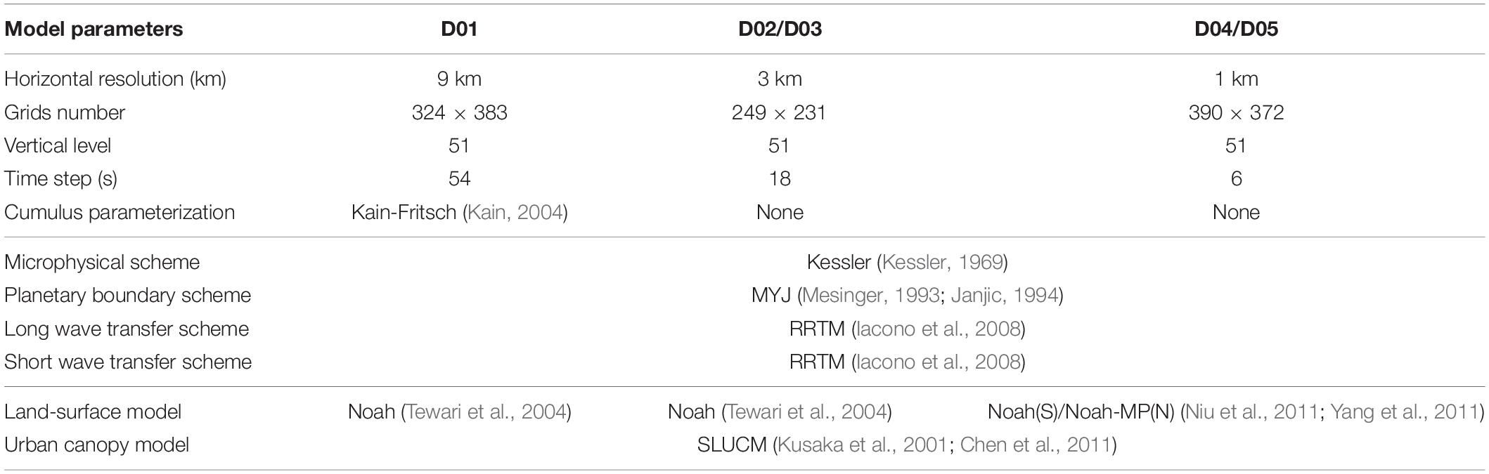
Table 1. The main parameters used in the WRF model setup.

Table 2. Urban canopy parameters used in this study.

Figure 1. (a) The nested simulation domains; (b) land cover for JJJ, and (c) PRD city cluster regions (red) in 2019, Beijing (BJ), Tianjin (TJ), Guangzhou (GZ), and Shenzhen (SZ) cities are marked; (d,e) the impervious surface ratio maps; (f,g), the high-, medium-, and low-density cities retrieved from impervious surface ratio for PRD (left) and JJJ (right). In panels (b,c), the black shaded regions show the terrain north of PRD and northwest of JJJ, while red, blue, and gray indicate urban, water body and other land uses. In panels (f-g), red, yellow, and blue denote high-, medium-, and low-density cities. The diurnal cycle coefficients of panels (h) ASH and (i) ALH in high-, medium-, and low-density cities. By acting on AH values in Table 3, these coefficients are used to produce gridded ASH and ALH (W m–2) values in high-, medium-, and low-density cities, characterized by diurnal variation, to be added into the model.
Data
Metrological Data
In this study, multi-metrological data support observation analysis and numerical simulation were performed. The European Center for Medium-Range Weather Forecast (ECMWF) ERA5 hourly reanalysis data, with a spatial resolution of 0.25 degrees and 37 pressure levels vertically extending from 1,000 to 1 hPa, were used to drive the WRF simulation as initial and boundary conditions. Also, from the ERA5 data, we described the general synoptic situation during a heat stress episode. The humidity and temperature profiles of the PRD and JJJ target regions were depicted from upper-air sounding observation. Surface automatic weather station (AWS) observations were performed to implement model verifications.
Land Use Data and Impervious Surface Map
We adopted the Moderate-resolution Imaging Spectroradiometer (MODIS) land use/land cover data from 2019 (Figures 1b,c). In addition, taking the heterogeneity of urban land cover into account, we further classified urban land use (Figures 1b,c) into high-/medium-/low-density types (Figures 1f,g), retrieved according to the percentage of impervious area. Herein, we took the percentage thresholds of 80 and 50% to identify high-/medium-/low- density urban areas and referred to Tewari et al. (2007) and Zhang et al. (2017b). To test inversion validity, global 30m impervious surface maps, amplified in the PRD and JJJ regions (Figures 1d,e), were also plotted. They were derived from multisource and multitemporal remote sensing datasets with the Google Earth Engine platform developed by Zhang et al. (2020). By contrast, the high-intensity urban areas, as shown in Figures 1f,g, matched well with impervious surface-dominant regions (Figures 1d,e).
Anthropogenic Heat Emission
The importance of AH in changing the near-ground energy balance as a heat source has been recognized (Oke, 1988; Grimmond, 1992; Sailor, 2011; Sailor et al., 2015; Chrysoulakis et al., 2016). AH is wasted heat in the form of sensible and latent heat due to human activities, and is released to an urban canopy (Yang et al., 2015; Yang W. et al., 2017). However, most studies have assumed that anthropogenic heat is sensible in nature without accounting for the latent heat component. Several studies have suggested that water vapor emission by cooling systems constitutes a substantial portion of latent heat flux in urban areas (Sailor et al., 2007; Miao and Chen, 2014), and this flux was shown to exceed 500 W m–2over central Tokyo in summer (Moriwaki et al., 2008).
In the current WRF-SLUCM system, both the ASH and ALH components of AH are considered. We adopted local AH releases (Table 3) over Chinese cities (Miao and Chen, 2014; Yang et al., 2015; Chew et al., 2021; Peng et al., 2021), replacing the default value modeled in WRF to improve HS simulation. The diurnal cycles of ASH and ALH (W m–2) in high-, medium- and low-density cities were added into the model by diurnal profiles coefficient (shown in Figures 1g,i) acting on the AH values shown in Table 3. Two peaks of ASH have coincided with local rush hours (8–9 and 17–18 LST), consistent with the default profile in the model and the bimodal mode of diurnal ASH profiles over the south and north Chinese cities (Wang and Wang, 2011; Wang et al., 2016). While the ALH profile was derived by combining Beijing-325 m weather tower observation analysis with land surface model (Miao and Chen, 2014), the diurnal variation of ALH flux followed the schedule of human activity and was relatively independent of season (Moriwaki et al., 2008). Both ASH and ALH were gradually strengthened on the heels of an increase in city density. Thereinto, the ASH flux in south cities exceeded the maximal value in Guangzhou (approximately 50 W⋅m–2), which has been recently estimated by Zhu et al. (2017).

Table 3. ASH and ALH releases in high-/medium-/low-density urban areas used in this study. The diurnal cycles of ASH and ALH (W m–2) profiles in high-, medium- and low-density cities refer to Figures 1g,i.
Experiment Design
We conducted numerical experiments in two groups (Table 4) to quantify how heat stress responds to AH release and increases in city size. By evaluating the contributions of temperature and humidity changes to HS change, the attribution to HS change was further dissected.
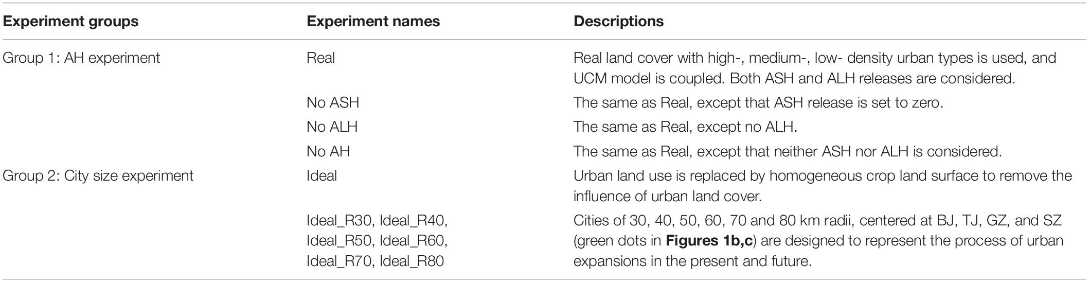
Table 4. Experiment design and description in section “Experiment Design.”
In the first group, we conducted four sets of experiments, which were named as Real, no ASH, no ALH, and no AH. All runs took the high-/medium-/low-density urban types of the current land cover into account. Meanwhile, reasonable AH ejections (including both ASH and ALH releases) were coupled into WRF by the SLUCM for the Real run. Then ASH run, ALH run, or both (i.e., total AH) were set to zero in turn to perform other simulations. By contrasting each run with Real run, we quantified the response of HS to each contributor. Additionally, the occurrence probabilities of EHSs in various-type urban regions were explored under different AH release scenarios.
We conducted the second group experiment to focus on how a gradual increase in city size influences heat stress intensity by utilizing the Real atmosphere idealized land-surface (RAIL) method (Schmid and Niyogi, 2013). We also probe into that, the varied HS with urban expansion is mainly determined by which driving factor, temperature change or humidity change. For the two target regions, Guangzhou (GZ) and Shenzhen (SZ) in the PRD region and Beijing (BJ) and Tianjin (TJ) in the JJJ region were selected to represent inland and coastal cities in south and north China (Figures 1b,c). In the Ideal run, urban land uses are replaced by the homogeneous crop land surface (i.e., the nearby rural land cover type), to remove the influence of urban land cover. Then, cities of 30, 40, 50, 60, 70, and 80 km radii (centered by green dots in Figures 1b,c) are designed to represent the process of urban expansions in the present and future. Refer to Schmid and Niyogi (2013) in which cities of different radii with the simplified, homogeneous land surface are designed to represent current and future city scenarios. The experiment results were used to perform comparative HS studies among inland and coastal cities in the south and north China.
Methods to Evaluate Temperature–Humidity Dependence for Heat Stress
Moist Enthalpy and Moist Entropy
Due to the high-temperature and high-humidity features of heat stress weather, two moisture-thermal energy metrics (Lutsko, 2021), moist enthalpy (H = CpT + Lqv) and moist entropy (S = Cplnθe) were introduced to differentiate the different characteristics during a heat stress episode in the PRD and JJJ city clusters. They included both temperature and humidity factors. And we are easily to separate temperature change from humidity change based on moist entropy or moist enthalpy formula, to evaluate their respective contributions to heat stress variation.
Moist entropy and moist enthalpy are classic thermodynamic variables in meteorology. Despite not being frequently used for heat stress compared to other several commonly used metrics, their application potentials as HS metrics and clear advantages in dynamics attract us to use them as indicators to discuss HS in this study. Note that in this study we did not attempt to determine the best way to measure heat stress. Rather, we examined whether moist enthalpy and entropy could be evaluative metrics to demonstrate an HS episode besides the three other widely used HS metrics. (1) By contrast between them and other commonly used HS indicators, we will evaluate the validities of moist entropy and moist enthalpy as metrics to characterize HS evolution to further prove their application potentials for HS weather. (2) They are classic thermodynamic and dynamic variables in meteorology. Taking moist entropy as an example, it has conservation property for a moistly adiabatic and frictionless atmosphere. Thus, it could be used as a mass surface or a tracer to demonstrate the convergence and dispersion of high-temperature and high-humidity atmosphere, so as to illustrate the genesis and diffusion of HS weather. In this regard, it is convenient to extend dynamically to further give mechanism responsible for HS weather and as a predicative factor in our follow-up study. (3) It is easy to separate the contributions of humidity change from temperature change by taking the differential operator on the moist entropy formula. Thus, by calculating and comparing the magnitudes of temperature and humidity changes, which one is the primary driver of the moist entropy fractional change will be judged. The entire separation and comparison do not depend on some subjective and empirical parameters, such as clothing index, exposure index, medical discomfort index, etc. This is easy to implement based on observations and numerical model. In terms of these, in this study, we mainly used moist enthalpy and especially moist entropy as indicators to discuss heat stress:
Where T and qv are absolute temperatures and specific humidity, Cp is the specific heat of dry air at constant pressure p. L is latent heat of vaporization and is equivalent potential temperature (Holton and Hakim, 2013). Herein, TL is the temperature at the lifting condensation level.
Methods to Separate Temperature–Humidity Contribution to Heat Stress
By taking the differential operator on the θe formula, we have [Eq. (1)], wherein the relation is used after analyzing the order of magnitude (Yang S. et al., 2014). In the near-surface level, surface pressure change is small, therefore fractional change in potential temperature (Δθ) is roughly equal to fractional change in temperature (L/CpΔqv) in Eq. (1). Thus, by calculating and comparing the magnitudes of Δθ and L/CpΔqv, which one (temperature or humidity change) is the primary driver of the θe fractional change will be judged.
Other Metrics to Evaluate Heat Stress Weather
Furthermore, additional several commonly used heat stress metrics (Steadman, 1994; Willett and Sherwood, 2012; Buzan et al., 2015), such as Humidex to compute the “feels-like” temperature for humans (), apparent temperature (AT, where AT = Tc + 0.33e−0.7u10m−4), simplified SWBGT, where (SWBGT = 0.56Tc + 0.393e + 3.94), were adopted to strengthen the validity of moist enthalpy and moist entropy as metrics to characterize heat stress events, where Tc and e are air temperature and vapor pressure in units of degrees Celsius and hPa, u10m is the 10-m speed wind, and e is calculated by relative humidity and saturated vapor pressure.
Results
Model Validation
Figures 2A–H compare the simulated (red) 2-m air temperature (Figures 2A–D) and relative humidity (Figures 2E–H) with observations (blue) derived from multi-stations over the region of the four cities. All these observations are from the national surface AWSs system network, with station locations shown in Figure 3.
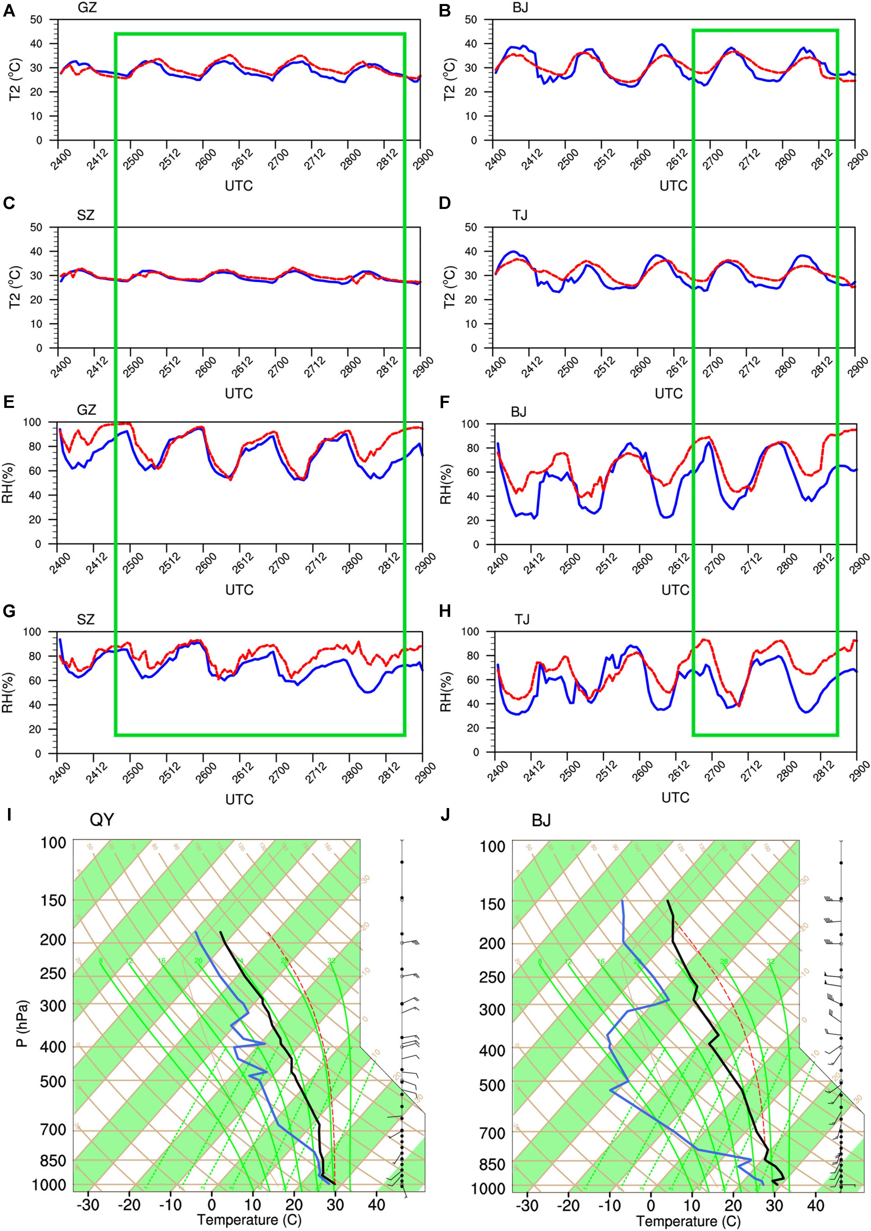
Figure 2. (A–H) Observed (red) and simulated (blue) 2-m air temperature (°C) and relative humidity (%). The green frames show the heat stress episodes in south and north cities. Sounding plots in panels (I) Qingyuan (QY) and (J) Beijing (BJ) stations, denote observations in south and north, with black and blue curves representing temperature and dew point, respectively.
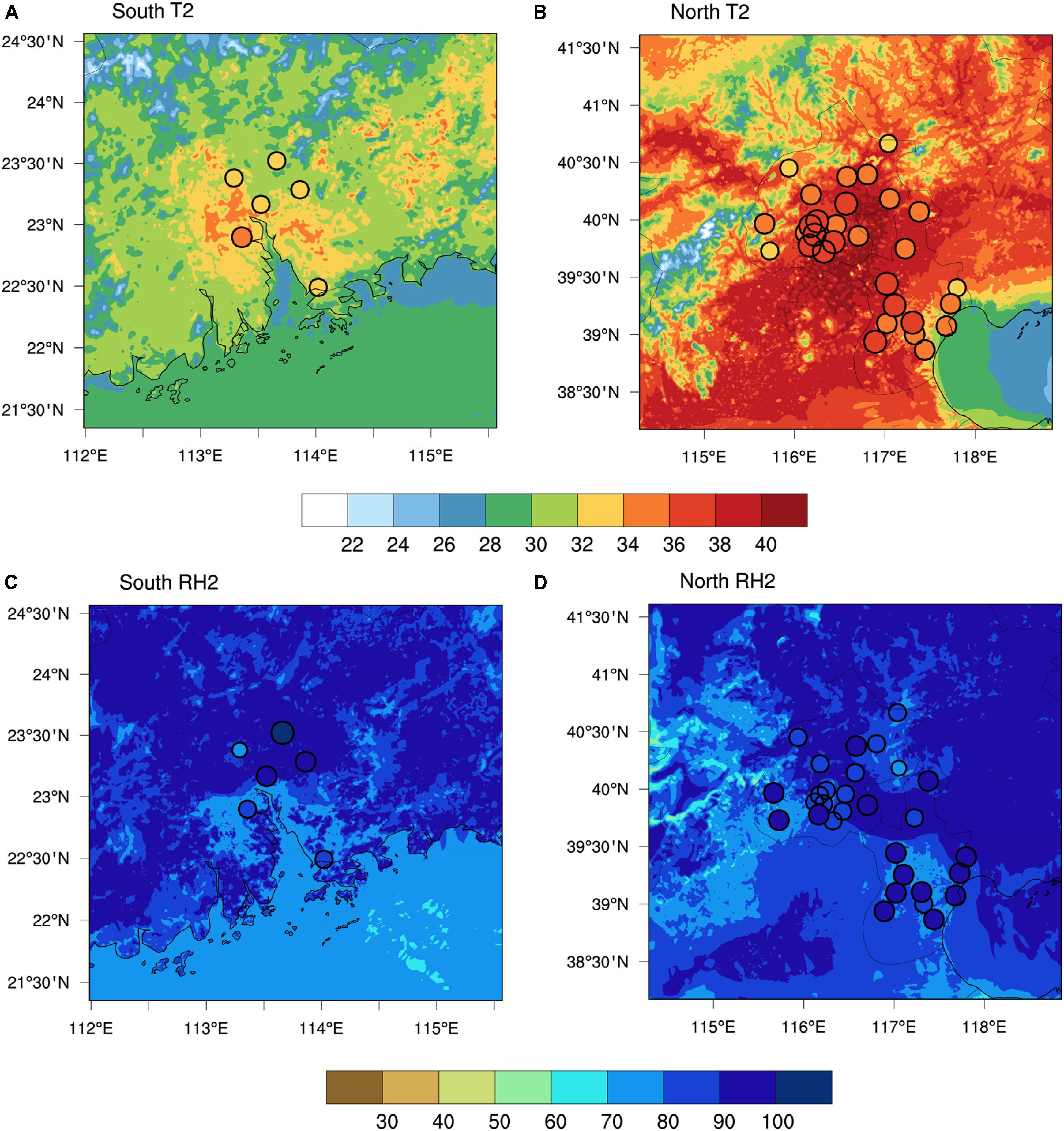
Figure 3. (A–D) The spatial charts of observed (shaded circles) and simulated (shaded) 2-m air temperature (°C) at 05 UTC and relative humidity (%) at 21 UTC 27. All these observations are from the national surface AWS system network, with station locations shown by circles. Where the shaded circles have sizes proportional to temperature and humidity (cf. the color scales below A-D).
According to the criterion of heat stress weather issued by China Meteorological Administration, a 4-day episode in PRD (01 LST 25-00 LST 29, i.e., 17 UTC 24-16 UTC 28) and a 2-day episode (01 LST 27-00 LST 29, i.e., 17 UTC 26-16 UTC 28) in JJJ are selected (framed by green boxes in Figures 2A–H) as examples to perform a comparative study for typical summer urban heat stress between the south and north cities of China. They generally satisfy the HS criterion that daily maximum temperature is more than 32°C. Meanwhile, the mean daily relative humidity (RH) is not less than 60%, and the weather process lasts at least 2 days.
The model performs well in reproducing the diurnal cycles (Figure 2) and spatial distributions (Figure 3) of near-surface air temperature and humidity during heat stress episodes (within green boxes), two key factors to evaluate heat stress intensity. It is remarkable that the simulated and observed diurnal peaks of temperature and humidity show a good agreement, despite slightly lower humidity simulations (Figures 2E-H). By comparing the observations between south and north cities (Figures 2, 3), higher humidity (e.g., nearly 100% in GZ) and relatively lower temperature (∼about 2–4°C difference) present in south (e.g., temperatures of GZ and SZ exceed 36 and 34°C, while maximal temperatures of BJ and TJ reach up to 38 and 37°C, respectively). From simulations, the comparative results among south and north cities are also reasonable, which have similar tendency with observations.
The root-mean-square error for all stations over the GZ, SZ, BJ, and TJ city regions are shown in Table 5. Overall, the simulation is improved by adding AH release (cf. Real and no AH runs in Table 5) and is comparable with previous studies (Meir et al., 2013; Ramamurthy and Bou-Zeid, 2017), which is directly attributable to the upward AH flux into UCM model. A certain degree of improvement presents, as ASH or ALH is considered alone (by comparing no AH with no ASH or no ALH run), but the improvement is most pronounced when both factors are considered.

Table 5. Root-mean-square errors of simulated air temperature (oC) for all stations over various city regions.
The general synoptic situation during the heat stress episode is briefly described. In the near-surface level, weak southerly (with region-mean intensity of wind speed less than 2 ms–1) prevails in PRD, bringing moisture from the ocean to the target region (not shown). In the JJJ region, southerly dominates Beijing, leading to positive temperature advection from south China; while easterly presents in coastal Tianjin, convenient to moisture transport from eastern ocean to JJJ. We also address the synoptic chart extending upward into the troposphere. A deep-layer high-pressure system caused by the in-phase superposition of middle-level subtropical high and low-level ridges, sinking motion, and weak southerly or easterly near surface, coacton HS weather. From the observed sounding plots (Figures 2I,J), stable stratification (black curve, denoted by temperature) inhibits vertical mixing under the boundary layer, which plays a key role in the formation of HS. High dew point (blue curve) indicates high humidity, especially in the south (Figure 2I), and a high-humidity pattern stretches up toward the whole troposphere, manifesting as approached temperature and dew point profiles. In the north (Figure 2J), large humidity presents in a low level. It decreases swiftly above 800 hPa, characterized by abruptly depressed dew point. All these provide favorable environments to HS weather.
Heat Stress Metrics
Several metrics are utilized to demonstrate the heat stress evolution, as shown in Figure 4. First, three commonly used heat stress metrics (Steadman, 1994; Willett and Sherwood, 2012; Buzan et al., 2015), AT, Humidex, and SWBGT (blue, green, and black curves in Figure 4), could effectively define the heat stress periods in the south and north cities (see the green boxes as shown in Figure 2) and reflect the HS characteristics of high temperature and high humidity. Second, moist enthalpy and moist entropy (H and S, purple and red curves in Figure 4), recently utilized by Lutsko (2021), are evaluative metrics to heat stress, since their evolution follow similar tendencies with other three metrics, except that they have larger value (∼370 K of moist entropy) in magnitude relative to AT, Humidex, and SWBGT (∼50°C below). In addition, consistent with SWBGM and AT, moist entropy and moist enthalpy over BJ and TJ in north China (Figures 4B,D) show more obvious diurnal variations compared with HS over GZ and SZ in south China (Figures 4A,C). Note that albeit there are strong HS signals in BJ for the 3rd day (01 LST 26-00 LST 27, i.e., 17UTC 25-16UTC 26), which is derived from little higher simulations for T2 and RH (Figures 2B,F). Since the observed daily mean humidity does not reach the HS criterion, we mainly concern the latter 2 days as HS episode in northern cities. The peak of HS present in the afternoon and early midnight (about 370 K for moist entropy, at about 06-12UTC) in north, while it takes on generally hot and moist in the south. For instance, the curves of moist entropy in GZ and SZ (Figures 4A,C) have less fluctuation than those in north cities (Figures 4B,D), maintaining a mean value above 360 K, which accords with our common sense and physical feelings.
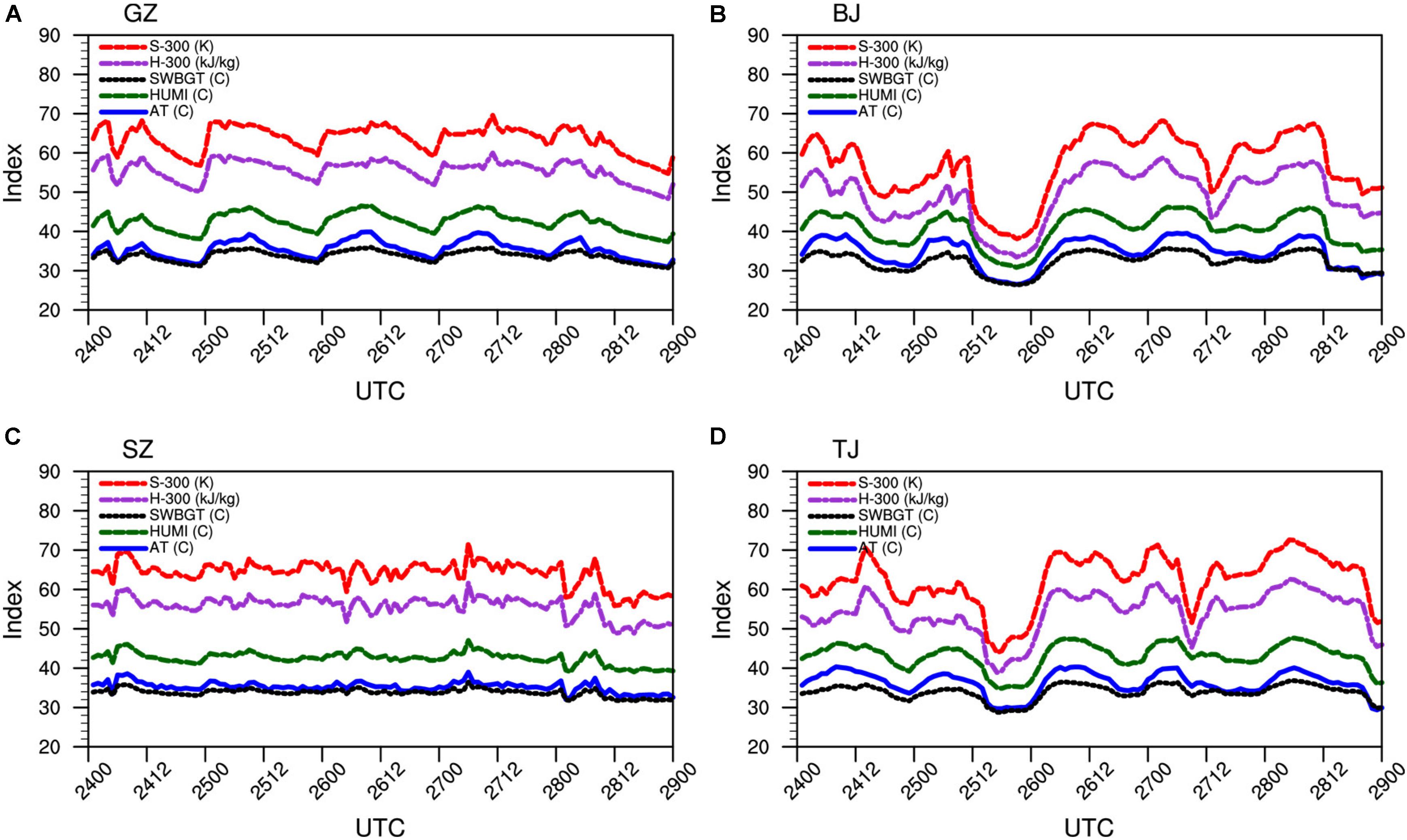
Figure 4. (A–D) Curves of five metrics to evaluate heat stress intensity evolution over GZ, SZ, BJ, and TJ city regions based on multi-station observations. Five metrics are apparent temperature (blue), Humidex (green), and simplified wet bulb globe temperature (black) (°C), moist enthalpy (H, purple) (K J/kg), and moist entropy (S, red) (K), respectively, where H and S minus 300 K in magnitude, to be comparable with other metrics.
Note that we do not attempt to determine the best way to measure heat stress here. Rather, we examine whether moist enthalpy and entropy could be evaluative metrics to demonstrate an HS episode, besides the other three widely used HS metrics. By contrast among metrics, we strengthen the validities of moist entropy and moist enthalpy as metrics to characterize HS evolution. The heat stress illustrates more extreme intensity and diurnal cycle in the north than in the south, for inland than for coastal cities. Of more importance is that it is easy to separate the key factors from each other (temperature and humidity herein) to drive heat stress change based on the moist entropy or moist enthalpy formula themselves. Therefore, we mainly utilize moist entropy or moist enthalpy as metrics to investigate the response of heat stress to AH and increase in city size, and to explain the attribution to HS change by separating the contributions of temperature and humidity changes in the subsequent analyses.
Impact of AH on HS
Pattern
Figure 5 shows the spatial distributions of moist entropy and moist enthalpy changes (ΔH and ΔS) due to AH and its components, and their pattern correlations with temperature and humidity changes (ΔT and ΔQ) for the group 1 experiment (Table 4). Variable R at the top of each panel denotes the correlation coefficient between its two subscript variables. By taking the difference between Real run and the other three runs, we quantify the sole influence of ASH (Real-no ASH), ALH (Real-no ALH), and AH (Real-no AH) in the south (Figures 5A–D) and north (Figures 5E–H), where gridding by slash line represents the urban region.
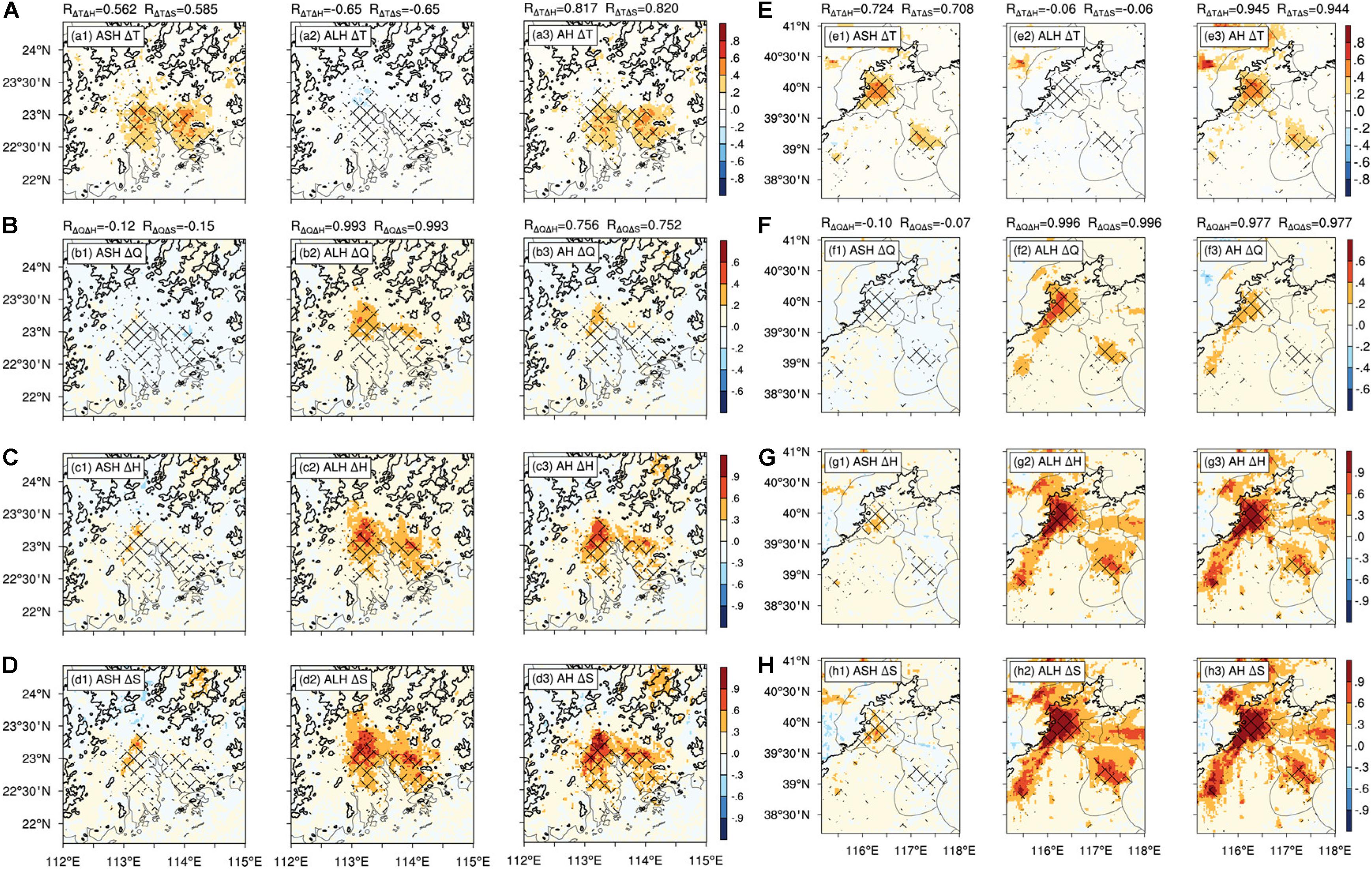
Figure 5. The spatial distribution of moist enthalpy and moist entropy changes (ΔH and ΔS) and their pattern correlations with temperature and humidity change (ΔT and ΔQ) for group 1 experiment (Table 2), taking account of the impact of AH and its components, and R at the top of each panel denotes the correlation coefficient between its two subscript variables. By taking the difference between Real run and the other three runs, we quantify the sole influence of ASH (Real–no ASH), ALH (Real–no ALH), and AH (Real–no AH) in south (A–D) and north (E–H), where gridding by slash line represents urban region.
From Figures 5a1–d1, the ASH effect leads to UHI (Figure 5a1) and UDI (Figure 5b1). However, their combination produces intensified urban heat stress (Figures 5c1,d1). In contrast to ASH, ALH (Figures 5a2–d2) has cooling (Figure 5a2) and humidifying (Figure 5b2) roles over the urban regions, which even produces more intense HS (Figures 5c2,d2) relative to the ASH effect (Figures 5c1,d1). Considering both components of AH (Figures 5a3–d3), AH makes the air over the urban region become hot (Figure 5a3) and moist (Figure 5b3) after neutralizing the contrary contributions of ASH (Figures 5a1,a2) and ALH (Figures 5b1,b2) effects on ΔT and ΔQ, which largely exacerbates heat stress (Figures 5c3,d3). This kind of aggravation of HS is particularly evident over the urban region (Figures 5c3,d3). The strong signals of positive ΔH and ΔS nearly outline the urban region. Comparing ASH (Figures 5c1,d1), ALH (Figures 5c2,d2), and AH effects (Figures 5c3,d3), the ALH accounts for larger proportion of total AH to strengthening HS.
In north cities (Figures 5E–H), the case is similar to that in south cities (Figures 5A–D), except for enhanced HS induced by stronger ASH effect (cf. Figures 5c1,d1,g1,h1), which produces stronger UHI in north than in south (cf. Figures 5a3,e3). In short, compared with the ASH component (Figures 5c1,d1,g1,h1) among total AH (Figures 5c3,d3,g3,h3), ALH (Figures 5c2,d2,g2,h2) has more significant impact on HS change. However, the contribution of ASH to HS change increases in north (Figures 5g1,h1), relative to that in south cities (Figures 5c1,d1).
As for spatial distribution, moist entropy and moist enthalpy present similar patterns of HS growth due to the AH effect over the urban regions (cf. Figures 5c3,d3,g3,h3). Both temperature and humidity changes have better pattern correlation with HS change in the north. For example, the correlation coefficients RΔTΔS (/RΔQΔS) between ΔT(/ΔQ) and moist entropy change (ΔS) reaches up to 0.944(/0.977) for the AH effect experiment (Figures 5e3,f3), indicative of strong dependence of HS change on both temperature and humidity change in the north. While in the south, the spatial pattern of HS change due to AH release is determined mostly by the coverage of UHI (RΔTΔS = 0.820), relative to humidity change distribution (RΔQΔS = 0.752).
Diurnal Variation Features
In consideration of clear diurnal cycles of ASH and ALH profiles (Figures 1h,i), diurnal variation features of how heat stress intensity responds to AH and its components are also demonstrated (Figures 6A–I), indicated by both heat stress metrics (Figures 6G–I) and temperature–humidity meteorological variables (Figures 6A–F). From Figure 5, the spatial patterns of ΔH and ΔS give strong signals in GZ and BJ (Figures 5c3,d3,g3,h3), indicative of a remarkable HS response to the AH effect. Thus, as typical cities in the south and north, GZ and BJ are chosen to illustrate the diurnal variation features of HS response to AH release.
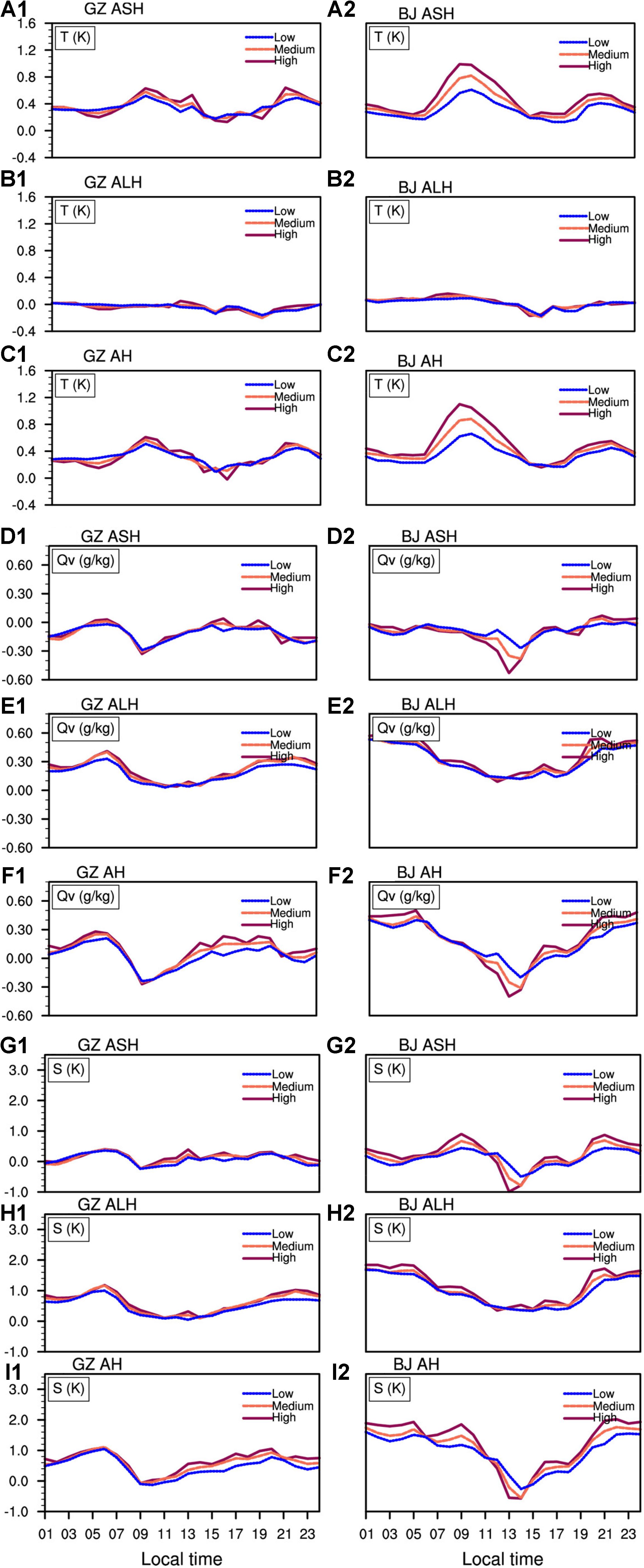
Figure 6. (A-I) The diurnal variations of temperature (K), humidity (g/kg), moist entropy (K) in high-/medium-/low-density urban areas (dark red/light red/blue) due to ASH, ALH, AH release. The curves denote the difference fields between Real run and other experiments (refer to Group 1 experiment in Table 4). Left and right panels are GZ and BJ, respectively.
Impacts of AH on meteorological variables are investigated first. Near-surface air temperature and humidity changes are plotted, as shown in Figures 6A–F, to explain the attributions to HS change (Figures 6G–I). Consistent with previous studies (e.g., Nie et al., 2017; Li et al., 2018), ASH heats the atmosphere by 0.2–1.2°C (Figures 6A1,A2), more pronounced in BJ than in GZ, with two peaks matching the ASH profile, as shown in Figure 1h, while ALH slightly cools T over the urban regions during daytime (Figures 6B1,B2), associated with human activities. Irrigated parks, greenbelt, highway sprinkling operation generate cooling but comparatively little (0.2°C). After partly offsetting between ASH and the ALH effect, ASH among total AH contributes most of urban heating. Consequently, UHI is determined mainly by ASH rather than ALH. Its peak reaches 0.6°C in south and 1.1°C in north cities (Figures 6C1,C2), with increased heating as the density of urbanization increases (e.g., mean ΔT>0.5°C between high- and low-density cities in BJ).
As for humidity change due to AH and its components (Figures 6D-F), UDI from ASH through decreased ΔQv (Figures 6D1,D2) is partly neutralized by the humidifying effect from ALH (Figures 6E1,E2). The ASH dries air, responsible for ΔQv < 0, as shown in Figures 6D1,D2; while the ALH moistens air, directly leading to ΔQv > 0, as shown in Figures 6E1,E2, which is consistent with the spatial pattern, as shown in Figures 5b1,b2,f1,f2. The changes in ΔQv as shown in Figures 6F1,F2, can be explained via a combination of ASH and ALH effects on humidity change. In brief, the ΔQv > 0 tendency maintains for the diurnal cycle in GZ, and the curve has two peaks (Figure 6F1). One happens during nighttime because of decreased evaporation loss, and then humidity decreases with sunrise. The other presents in the afternoon because of ALH from irrigation and watering park, etc. However, the ΔQv > 0 trend is broken down in the afternoon in BJ (Figure 6F2), even if the ALH peak synchronously presents in the afternoon (Figure 1i). Under higher-temperature conditions in the north, dramatic evaporation dries down the near-surface moisture, responsible for the afternoon humidity deficit (Figure 6F2).
The impact of AH on heat stress metrics are analyzed and shown in Figures 6G–I. Since the impact of three AH releases’ strategies on the pattern (cf. Figures 4C,D, or cf. Figures 4G,H) and diurnal cycle of moist enthalpy (not shown) resemble those of moist entropy (Figures 6G–I), we examine moist entropy as an example (Figures 6G–I).
The AH effect has a substantial impact on the heat stress index. Both ASH and ALH (Figures 6G,H) could aggravate the HS (Figure 6I), with a maximal increment of moist entropy about 1 K at 06/20 LST in GZ and 09/21 LST in BJ. Furthermore, the magnitude of the HS index increases with the density of urbanization. In contrast of south and north HS, there is a larger diurnal variation in BJ (Figure 6I2), even decreased HS between 12 and 16LST. It means that sprinkling water on the road under high-temperature conditions (Figure 6C2) might alleviate HS in north cities. The additional irrigation increases the amount of moisture in the air. A large amount of evaporation takes away excessive heat, reducing near-surface temperature and therefore alleviating HS. In contrast, it does not work to sprinkle water on roads or gardens in southern cities, from the positive contributions of both ASH and ALH (Figures 6G1,H1) to HS aggravation (Figure 6I1).
Impact of City Size on HS
Pattern
Figure 7 shows the spatial distributions of HS changes (ΔH and ΔS) due to an increase in city size and their pattern correlations (R) with temperature and humidity changes (ΔT and ΔQ) for the group 2 experiment in Table 4. By taking the difference between Ideal run and the other six simulations with varied city radii from 30 to 80 km, we evaluate HS scenarios in present and future in south (Figures 7A–D) and north (Figures 7E–H), wherein slash line regions indicate urban coverage.
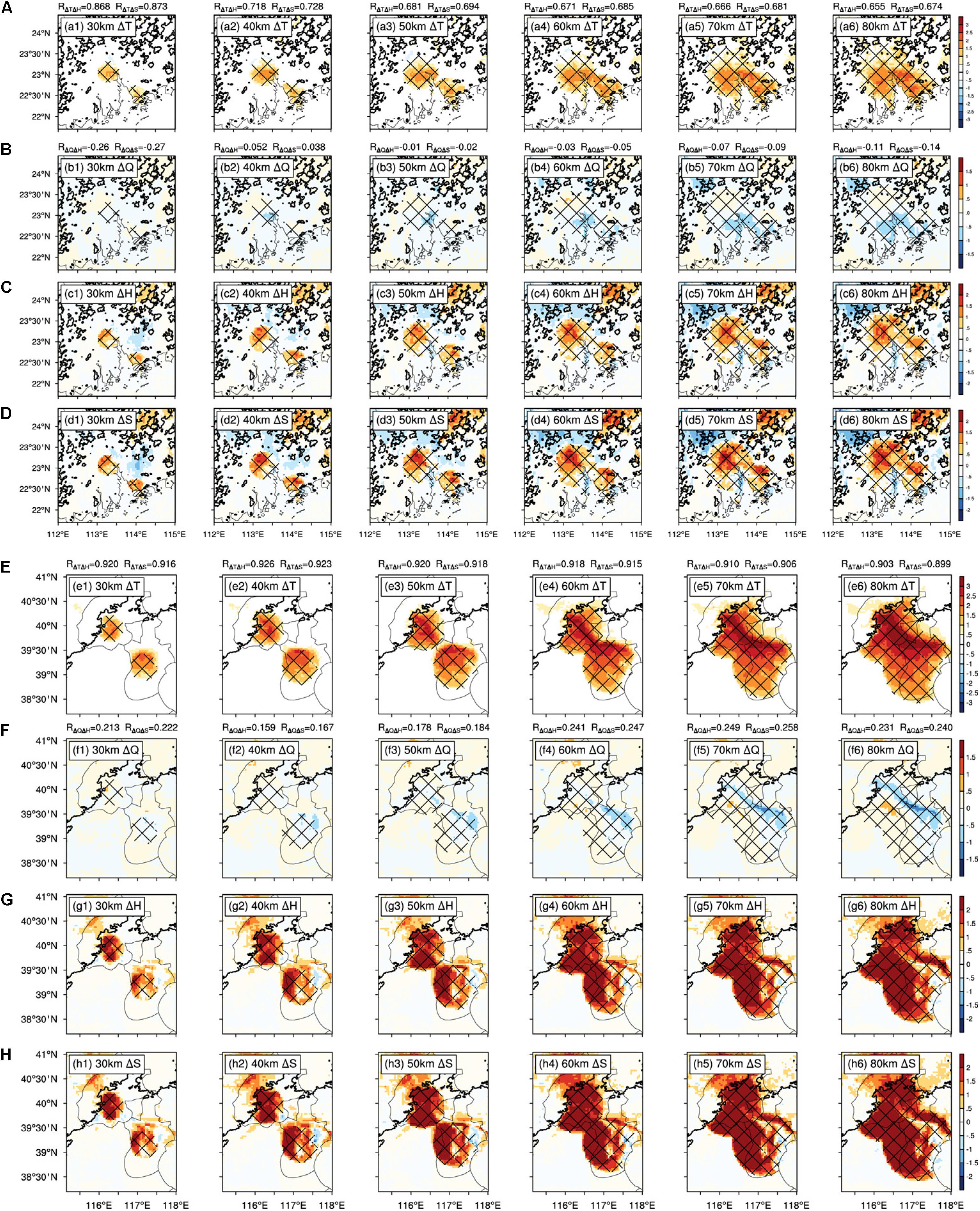
Figure 7. (A-H) The same as Figure 5 but for group 2 experiment in Table 4 by taking account of the impact of increasing city size from R = 30 to 80 km.
From Figures 7A–D, UHI and UDI are remarkable over the urban regions. ΔT and ΔQ are almost in opposite-phase distributions. The coverage of UHI and UDI presents a dramatic extension with the expansion of the city, as shown in Figures 7a1–a6, b1–b6. After neutralizing the contrary contributions of UHI (Figures 7a1–a6) and UDI (Figures 7b1–b6) effects, we depict the HS evolution with urban sprawl (Figures 7c1–c6,d1–d6). It can be seen that the extension of HS coverage is also pronounced as an urban area grows. Strong HS covers an urban region well, except to the northeast of the PRD region, because of downwind heat accumulation by thermal advection originating from upstream urban. However, the enhancement of HS intensity is not as significant as that of UHI because of anti-phase synchronous growths of positive/negative contribution of UHI/UDI to HS. In contrast, the case in north cities (Figures 7E–H) is similar to that in the south (Figures 7A–D), except for intensified HS induced by stronger UHI (cf. Figures 7A,E) and weaker UDI (cf. Figures 7B,F) in the north.
Also, from the spatial distribution, temperature change has a large pattern correlation coefficient with HS change, about 0.9 for ΔT and ΔS in the north (Figure 7E) and >0.6 in the south (Figure 7A). However, the correlation coefficients between humidity change and moist entropy change RΔQΔS is small (<0.3) (Figures 7B,F). It indicates strong dependence of the HS pattern on temperature change due to urban expansion. If we build megacities, the temperature change will be the primary control on the spatial pattern of HS.
Intensity Change
The histograms in Figure 8 show intensity changes in UHI (yellow histogram), UDI (blue histogram), and UHS (grown curve) under R1–R6 city size scenarios in BJ, TJ, GZ, and SZ. Thereinto, we take the daily maximum of urban region averaged temperature rise and moisture depict relative to Ideal run without the city as UHI and UDI, and the maximal equivalent potential temperature change is adopted to estimate the UHS change.
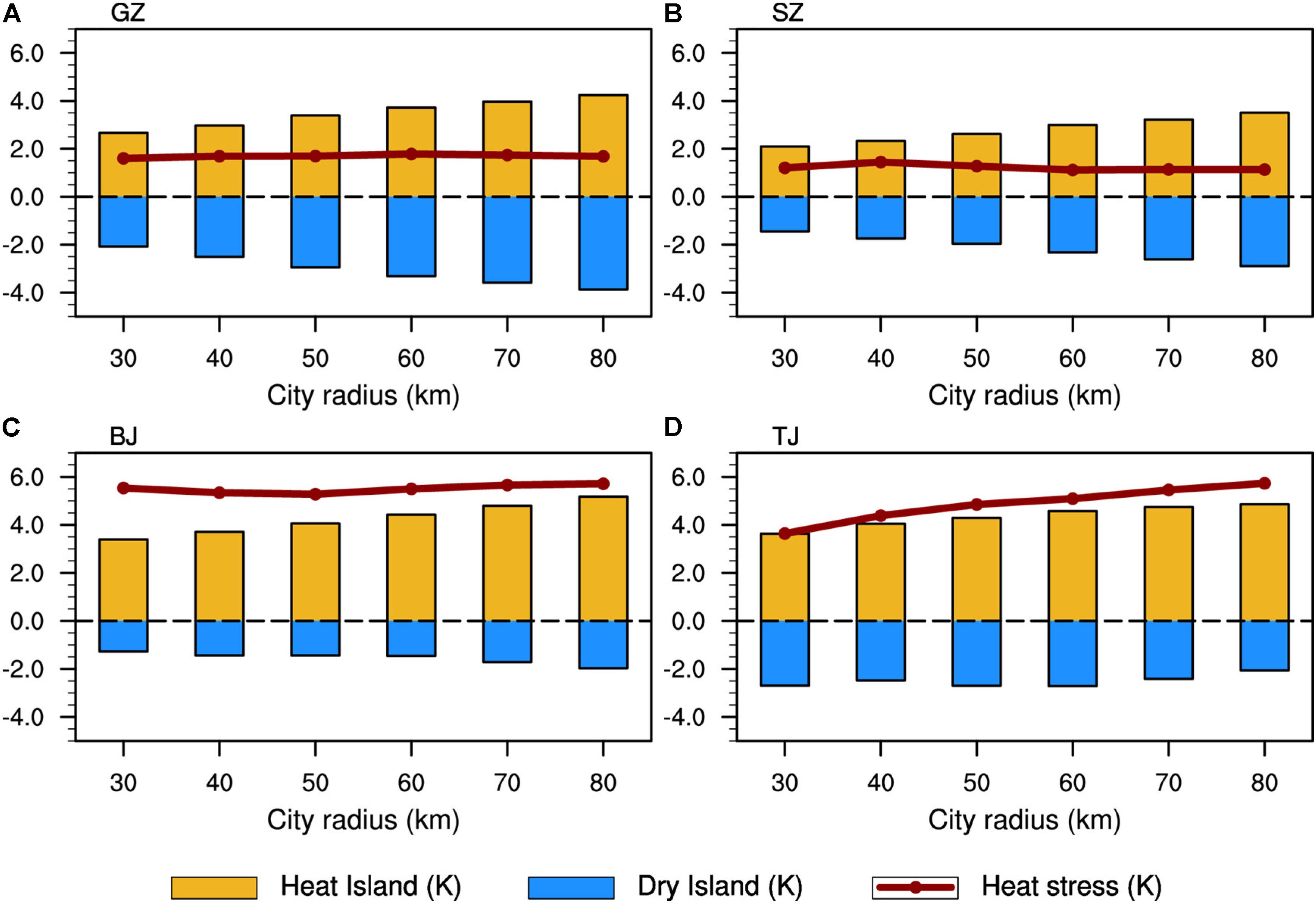
Figure 8. (A-D) Daily maximum of region-averaged urban heat island effect (Δθ, K, yellow histogram), urban dry island effect (moisture depict in K, L/CpΔqv, blue histogram), and urban heat stress change (Δθe, K, grown curve) under R1–R6 (R = 30–80 km) city size scenarios in BJ, TJ, GZ, and SZ city regions. The fractional changes (Δθ, L/CpΔqv, Δθe) are taken as difference between the R1–R6 experiment and Ideal run without city (refer to Group 2 experiment in Table 4).
We use the temperature-humidity separation method introduced in section “Methods to Separate Temperature–Humidity Contribution to Heat Stress” to assess the relative significance of temperature and humidity changes (UHI and UDI effects) on UHS change, by weighting Δθ and L/CpΔqv more heavily (Figures 8A–D). Note that the coefficient L/Cp is added into the moisture change factor, so as to produce comparable order of magnitude and equivalent unit to temperature change.
The heat stress change in south and north cities becomes complex via the combined effects of temperature and humidity changes due to urban sprawl. The UHS maintains less variation in the south in the progress of urban expansion, because of nearly simultaneous growth of the out-of-phase contributions due to UHI and UDI effects (Figures 8A,B). However, UHS experiences slow enhancements with the increase in city sizes in north cities (Figures 8C,D), mostly driven by the UHI effect. Thus, temperature change dominates the HS change due to urban expansion in north, but both temperature and humidity changes contribute equivalently to HS in the south. As expected, the contrast of environmental conditions between south and north China supports the above conclusion. It is generally wet and hot in the south, which produces large contributions of both temperature and humidity to the HS weather: while in the north, it is hotter but not as wet as in the south (Figure 2), so the temperature change dominates intensity evolution of HS. In contrast, stronger UHS change on account of increased urban area happens in the north, with a larger peak (∼6 K) relative to that in the south (∼2 K), and stronger HS presents over inland BJ/GZ than in coastal TJ/SZ. Also, note that the intensified HS over TJ (Figure 8D) and a little weakened HS over SZ (Figure 8B) due to growing city radius are associated with the urban sprawl toward inland and coastal areas. Therefore, it is more prone to severe UHS risk if we build megacities in the north in the future.
Extreme Heat Stress
Threshold of Extreme Heat Stress
To explore the EHS events, we try to derive a local threshold based on the statistical distribution mode of extreme heat stress metric, equivalent potential temperature herein. Referring to the CFAD (contoured frequency by altitude diagram) method widely applied to convective burst definition (Yuter and Houze Jr., 1995; Rogers, 2010; Heng et al., 2020), we examine the distribution pattern of equivalent potential temperature by using contoured frequency by latitude diagram (CFLD) (Figure 9).
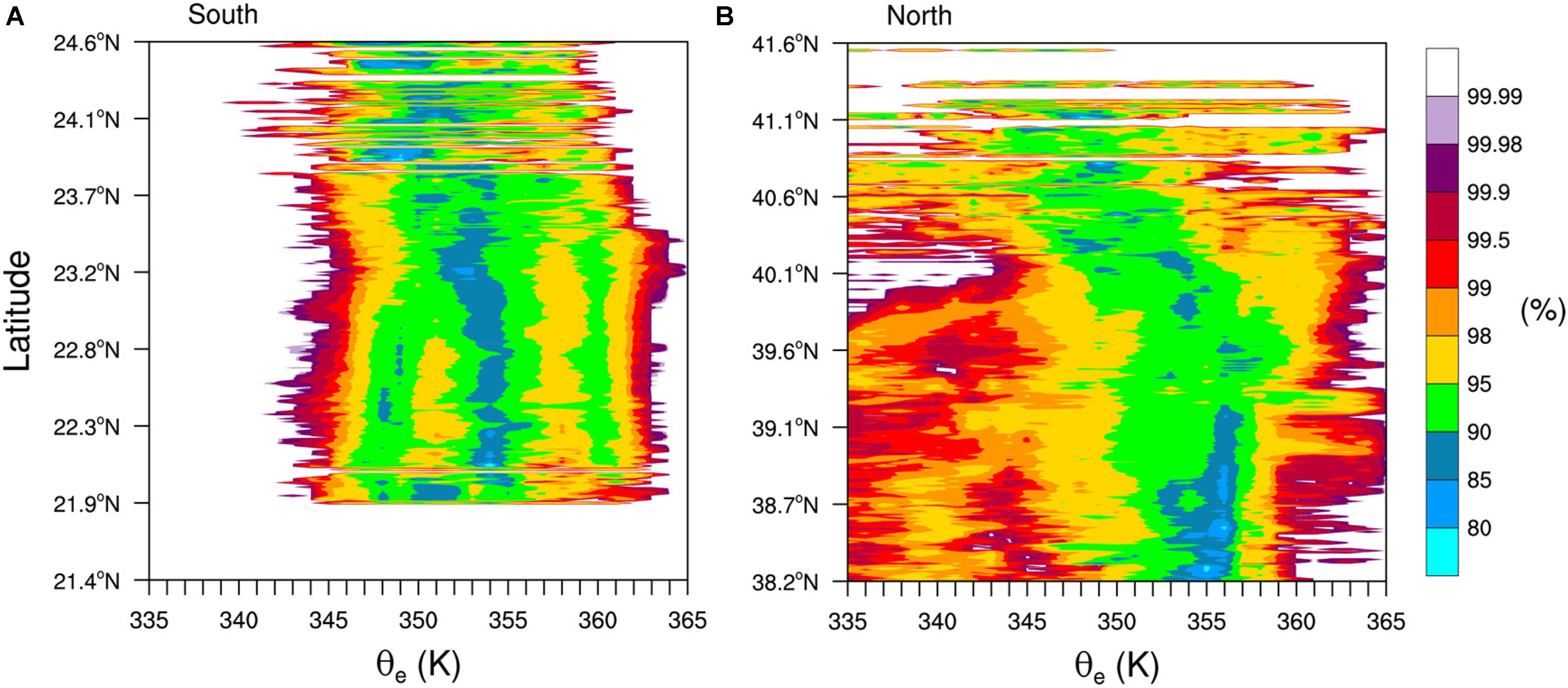
Figure 9. The contoured frequency by latitude diagram distribution of equivalent potential temperature (K) (A) in south and (B) in north.
It shows the CFLDs of the simulated equivalent potential temperature binned every 1 K at various latitudes within the PRD (Figure 9A) and JJJ (Figure 9B) regions based on Real run, where blank area represents sea or other non-urban land covers. By comparative analyses of the south and north cities (Figures 9A,B), the frequency distribution of equivalent potential temperature is relatively spatially homogeneous in the whole PRD region (21.9–23.7°N). All θe values concentrate within 343–363 K irrespective of varied latitude (Figure 9A), with peak θe (98th percentile, refer to Lutsko, 2021) of 362 K, while the frequency distribution of θe experiences dramatic amplification and is characterized by a broader mode (varied between 335 and 365 K) in JJJ, with peak θe (still 98th percentile) growing mainly from 359 to 362 K with latitude (Figure 9B). To be convenient to perform comparisons among various cities, we need to develop a common, unified standard to feature an EHS episode based on the statistical distribution of equivalent potential temperature in our target regions. It seems that 362 K is suitable to the extreme heat stress definition derived from θe statistics. Therefore, this criterion is attempted to analyze the EHS episode in the following section.
Temperature–Humidity Dependence
Figures 10, 11 are the scatter plots of Δθ (abscissa) and L/CpΔqv (ordinate) associated with EHS, which is used to study the relative importance of fractional changes in temperature and humidity on EHS occurrence under various AH release (Figure 10) and city size scenarios (Figure 11). By weighting Δθ and L/CpΔqv more heavily, we estimate which factor is the primary driver of EHS occurrence. Also shown is the θe value in high-/medium-/low-density urban regions (color triangle, star, dot in Figure 10) and cities with increasing size (color dot in Figure 11). It provides another way to estimate the sensitivity of EHS dependence on temperature–humidity change due to AH and increased city size by comparing whether the relative spread degree of EHS points is towards the abscissa or ordinate variables. The R value inset in each panel represents the hit ratio of EHS among total grids over the urban regions, with subscripts L, M, and H denoting low-/medium-/high-density city types.
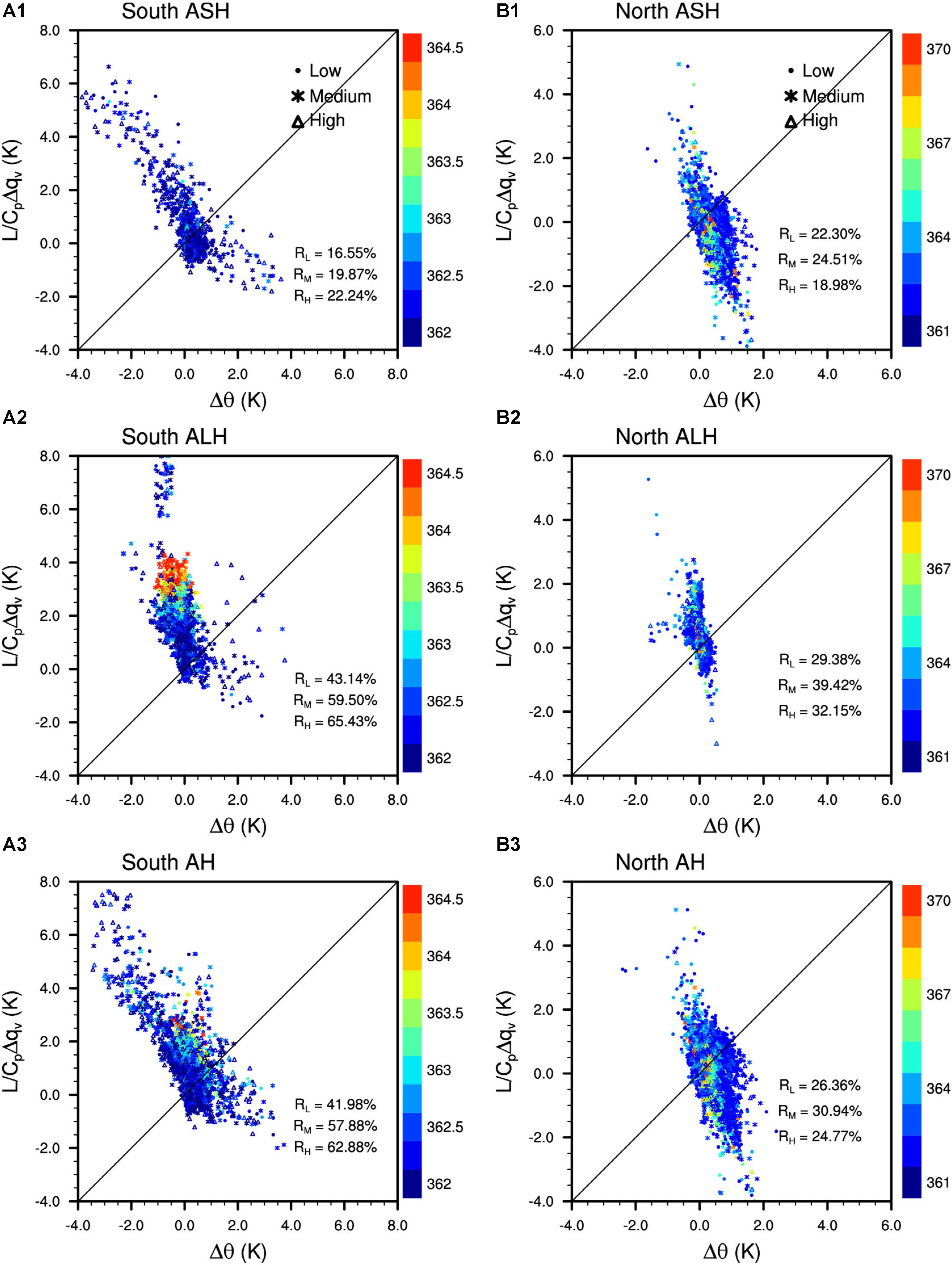
Figure 10. (A,B) Scatter plots of changes in humidity (L/CpΔqv, K) versus changes in temperature (Δθ, K) associated with extreme heat stress (98th percentile θe) events for the ASH, ALH, and AH runs. The triangle, star, and dot represent high-/medium-/low- density urban areas, colored by their associated θe value. Left and right panels denote south and north urban regions, respectively.
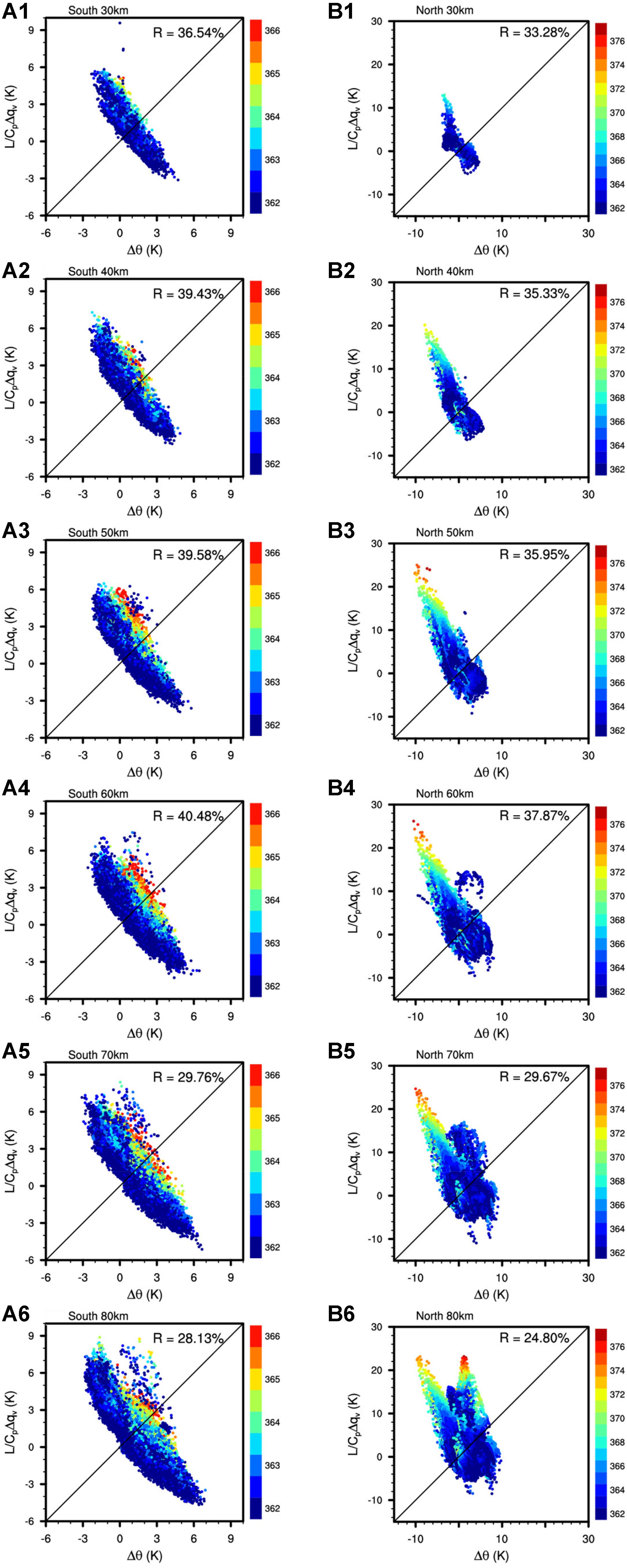
Figure 11. (A,B) The same as Figure 10 but for different city size (R1–R6) runs.
From Figure 10, the spread in humidity changes is larger than the spread in temperature changes in southern cities, irrespective of ALH, ASH, or AH run (Figures 10A1–A3), which signifies humidity change is the primary driving factor of EHS events in the south. In the north, the spread in humidity changes is larger/less than the spread in temperature changes in ALH/ASH run (Figures 10B1,B2), which implies humidity/temperature change is the primary driving factor of EHS events under an ALH/ASH release scenario. For AH simulation (Figure 10B3), the spread degrees in both factors are comparable, which means the occurrence of EHS is sensitive to both temperature and humidity increase over the north cities. In contrast, the hit ratios of EHS in high-/medium-/low-density urban are different. For the present urban land cover, considering various urban types and AH emission, above 50% (/a quarter of) south (/north) urban region is hit by EHS (Figures 10A3,B3), and EHS tends to occur in high-density urban regions in south, followed by medium-density urban regions (e.g., for AH run, as shown in Figure 10A3, RH = 62.88%, RM = 57.88%, and RL = 41.98%, indicating that 62.88% of the high-density urban regions is hit by EHS). However, EHS is more easily to happen in medium-density urban regions in all of the simulation experiments for north cities (e.g., for ASH, ALH, and AH runs, RM = 24.51, 39.42, and 30.94%, respectively).
As a city will expand dramatically in the future (Figure 11, and for group 2 experiment in Table 4), about one-third of the urban regions might be hit by EHS, with a wider scope of influence in the south than in the north (R = 28.13–40.48% in the south from Figures 11A1–A6, R = 24.80–37.87% in the north from Figures 11B1–B6). In addition, a larger extremum (with θe > 376 K) happens in northern cities, relative to that in the south (θe∼ 366 K). Furthermore, changes in the very warmest θe events are associated with large Δqv responses in north cities (Figures 11B1–B6). In the south (Figures 11A1–A6), EHS is sensitive to both temperature and humidity changes for smaller cities (Figures 11A1,A2), but the shift is to be determined by larger Δqv in the larger cities of the future (Figures 11A3–A6). For the EHS events in megacities in the south (Figures 11A3–A6), the specific humidity response is again the leading factor driving EHS occurrence in response to city size change. Therefore, constraining the probability of occurrence and regional distribution of EHS events largely comes down to constraining the humidity change associated with these events, particularly in a megalopolis or a city cluster in the future.
Conclusion and Discussion
The impacts of anthropogenic heat emission and increase in city size on urban heat stress and extreme heat stress are investigated based on numerical simulation by utilizing the coupled SLUCM-WRF model system. As effective HS metrics, moist enthalpy and moist entropy are used to evaluate the HS response to AH and urban expansion and explain the attribution to HS change by separating the contributions of temperature change from humidity change. Several main conclusions are summarized as follows.
Anthropogenic heat release could aggravate UHS drastically. It produces a maximal increment of moist entropy (an effective HS metric), above 1 and 2 K over south and north high-density urban regions, mainly through ALH. HS change shows a more prominent diurnal variation in the north than in the south, in high-density than in low-density urban regions. Despite the diurnal cycle of temperature/humidity rise due to ASH/ALH generally matching the ASH/ALH profile, HS change does not strictly obey the diurnal variation rule of any one single factor. It depends on the combined effect of both, indicative of the complexity of HS research. Note that there are slightly decreased HS between 12 and 16LST in the north in AH run, mainly by the ALH effect. It means that sprinkling water on roads under high-temperature conditions might alleviate HS in north cities. In contrast, it does not work to sprinkle water on roads or gardens in south cities, because of the positive contributions of both ASH and ALH to HS aggravation.
Urban expansion leads to an increase in HS coverage, and it has a larger impact on UHS intensity change (6 and 2 K in south and north) relative to AH. The city radius of 60 km is a possible threshold to plan to city sprawl. Above that city size, the HS intensity change due to urban expansion tends to slow down in the north and inhibit in the south (Figure 8), and about one-third of the urban regions might be hit by extreme heat stress (EHS), reaching maximal hit ratio (Figure 11). Stronger intensities of HS present over inland than in coastal cities. Therefore, it is more prone to severe UHS risk if we build megacities in the north in the future.
Furthermore, changes in warmest EHS events are more associated with high humidity change responses, irrespective of cities being in north or south of China, which supports the idea that humidity change is the primary driving factor of EHS occurrence. Therefore, constraining the occurrence probability and regional distribution of EHS events largely comes down to constraining the humidity change associated with these events, particularly in a megalopolis or a city cluster in the future.
In comparison to previous studies, Ramamurthy and Bou-Zeid (2017) performed a comparative analysis of heat waves over multiple cities. They found that UHI intensity is proportional to the physical size of the city. Based on this study, we quantify how the increase in city size impacts a heat stress episode and derive the threshold mentioned above in which this kind of influence will be slowed down. Yang et al. (2019) pointed out that urbanization increases thermal discomfort hours by 27% during summer over the urban areas of the Yangtze River Delta in East China, and that the contribution of AH to the increase in total discomfort hours is almost equal to that due to urban land use change. Our results reveal a stronger response of HS to urban expansion relative to AH in south and north cities in China. Furthermore, we demonstrate the influence path of AH on HS, mainly via its latent component but not the traditional anthropogenic sensible component. Certainly, updated numerical model setup, local UCM parameter, and densely gridded ASH and ALH data are expected to further simulate HS, and more thermodynamic and dynamic aspects based on conserved moist entropy are needed in the next study to reveal the mechanism responsible for the genesis and dispersion of HS.
Data Availability Statement
The original contributions presented in the study are included in the article/supplementary material, further inquiries can be directed to the corresponding author/s.
Author Contributions
SY and BC designed the research and led the writing of the manuscript. SL prepared all figures. ZX and JP performed the part data analysis. All authors discussed the results and commented on the manuscript.
Funding
The authors were supported by the National Natural Science Foundation of China (Grant Nos. 41875079 and 91937301), the Open Research Program of the State Key Laboratory of Severe Weather, Chinese Academy of Meteorological Sciences (2019LASW-A04), the National Key Research and Development Program on Monitoring, Early Warning and Prevention of Major Natural Disaster (2018YFC1506001), the Second Tibetan Plateau Comprehensive Scientific Expedition and Research Program (2019QZKK0105), and the S&T Development Fund of CAMS (2020KJ017).
Conflict of Interest
The authors declare that the research was conducted in the absence of any commercial or financial relationships that could be construed as a potential conflict of interest.
References
Allen, L., Lindberg, F., and Grimmond, C. S. B. (2011). Global to city scale urban anthropogenic heat flux: model and variability. Int. J. Climatol. 31, 1990–2005. doi: 10.1002/joc.2210
Buzan, J. R., Oleson, K., and Huber, M. (2015). Implementation and comparison of a suite of heat stress metrics within the Community Land Model version 4.5. Geosci. Model Dev. 8, 151–170. doi: 10.5194/gmd-8-151-2015
Chen, F., Kusaka, H., Bornstain, R., Ching, J., Grimmond, C. S. B., Grossman-Clarke, S., et al. (2011). The integrated WRF/urban modeling system: development, evaluation, and applications to urban environmental problems. Int. J. Climatol. 31, 273–288. doi: 10.1002/joc.2158
Chen, F., Yang, X., and Wu, J. (2016). Simulation of the urban climate in a Chinese megacity with spatially heterogeneous anthropogenic heat data. J. Geophys. Res. Atmosph. 121, 5193–5212. doi: 10.1002/2015jd024642
Chen, Y., Jiang, W. M., Zhang, N., He, X. F., and Zhou, R. W. (2008). Numerical simulation of the anthropogenic heat effect on urban boundary layer structure. Theoret. Appl. Climatol. 97, 123–134. doi: 10.1007/s00704-008-0054-0
Chen, Y., Jiang, W. M., Zhang, N., He, X. F., and Zhou, R. W. (2009). Numerical simulation of the anthropogenic heat effect on urban boundary layer structure. Theor. Appl. Climatol. 97, 123–134.
Chew, L. W., Liu, X., Li, X. X., and Norford, L. K. (2021). Interaction between heat wave and urban heat island: a case study in a tropical coastal city, Singapore. Atmosph. Res. 247:105134.
Chrysoulakis, N., Heldens, W., Gastellu-Etchegorry, J. P., Grimmond, S., Feigenwinter, C., Lindberg, F., et al. (2016). A novel approach for anthropogenic heat flux estimation from space IEEE International Geoscience & Remote Sensing Symposium. IEEE 2016, 6774–6777.
Feng, J.-M., Wang, Y.-L., Ma, Z.-G., and Liu, Y.-H. (2012). Simulating the regional impacts of urbanization and anthropogenic heat release on climate across China. J. Clim. 25, 7187–7203. doi: 10.1175/jcli-d-11-00333.1
Fischer, E. M., and Knutti, R. (2013). Robust projections of combined humidity and temperature extremes. Nat. Climate Change 3, 126–130. doi: 10.1038/nclimate1682
Grimmond, C. S. B. (1992). The suburban energy balance: methodological considerations and results for a midlatitude west coast city under winter and spring conditions. Int. J. Climatol. 12, 481–497.
Hass, A. L., Ellis, K. N., Mason, L. R., Hathaway, J. M., and Howe, D. A. (2016). Heat and humidity in the city: Neighborhood heat index variability in a mid-sized city in the southeastern United States. Int. J. Environ. Res. Public Health 13, 1–19. doi: 10.3390/ijerph1301010117
Heng, J., Yang, S., Gong, Y. F., Gu, J. F., and Liu, H. W. (2020). Characteristics of the convective bursts and their relationship with the rapid intensification of Super Typhoon Maria (2018). Atmosph. Ocean. Sci. Lett. 13, 146–154. doi: 10.1080/16742834.2020.1719009
Holton, J. R., and Hakim, G. J. (2013). An Introduction to Dynamic Meteorology, 5th Edn. Cambridge, MA: Academic Press.
Iacono, M. J., Delamere, J. S., Mlawer, E. J., Shephard, M. W., Clough, S. A., and Collins, W. D. (2008). Radiative forcing by long–lived greenhouse gases: calculations with the AER radiative transfer models. J. Geophys. Res. 113, D13103. doi: 10.1029/2008JD009944
Iamarino, M., Beevers, S., and Grimmond, C. S. B. (2012). High-resolution (space, time) anthropogenic heat emissions: London 1970–2025. Int. J. Climatol. 32, 1754–1767. doi: 10.1002/Joc.2390
Ichinose, T., Shimodozono, K., and Hanaki, K. (1999). Impact of anthropogenic heat on urban climate in Tokyo. Atmos. Environ. 33, 3897–3909. doi: 10.1016/S1352-2310(99)00132-6
Janjic, Z. I. (1994). The step-mountain eta coordinate model: further developments of the convection, viscous sublayer, and turbulence closure schemes. Month. Weather Rev. 122, 927–945.
Kain, J. S. (2004). The Kain-Fritsch convective parameterization: an update. J. Appl. Meteor. 43, 170–181. doi: 10.1175/1520-0450
Kessler, E. (1969). On the distribution and continuity of water substance in atmoshperic circulations. Meteor.Monogr 32:84. doi: 10.1007/978-1-935704-36-2_1
Kusaka, H., Kondo, H., Kikegawa, Y., and Kimura, F. (2001). A simple single-layer urban canopy model for atmospheric models: comparison with multi-layer and slab models. Bound. Layer Meteorol. 101, 329–358.
Lee, S. M., and Min, S. K. (2018). Heat stress changes over East Asia under 1.5° and 2.0°C global warming targets. J. Clim. 31, 2819–2831. doi: 10.1175/JCLI-D-17-0449.1
Li, S. W., Yang, S., and Liu, H. W. (2018). Sensitivity of warm-sector heavy precipitation to the impact of anthropogenic heating in South China. Atmos. Oceanic. Sci. Lett. 11, 236–245. doi: 10.1080/16742834.2018.1469952
Lorenz, R., Stalhandske, Z., and Fischer, E. M. (2019). Detection of a climate change signal in extreme heat, heat stress, and cold in Europe from observations. Geophys. Res. Lett. 46, 8363–8374. doi: 10.1029/2019GL082062
Luo, M., and Lau, N. C. (2018). Increasing heat stress in urban areas of eastern China: acceleration by urbanization. Geophys. Res. Lett. 45, 1360–1369. doi: 10.1029/2018GL080306
Lutsko, N. J. (2021). The relative contributions of temperature and moisture to heat stress changes under warming. J. Clim. 34, 901–917. doi: 10.1175/JCLI-D-20-0262.1
Meir, T., Orton, P., Pullen, J., Holt, T., Thompson, W., and Arend, M. (2013). Forecasting the New York City urban heat island and sea breeze during extreme heat events. Weather Forecast. 28, 1460–1477.
Mesinger, F. (1993). Forecasting Upper Tropospheric Turbulence Within the Framework of the Mellor-Yamada 2.5 Closure. Research Activities in Atmospheric and Oceanic Modelling. CAS/JSC WGNE Reper No. 18, Geneva: WMO, 28–24.
Miao, S. G., and Chen, F. (2014). Enhanced modeling of latent heat flux from urban surfaces in the Noah/single-layer urban canopy coupled model. Sci. China Earth Sci. 57, 2408–2416. doi: 10.1007/s11430-014-4829-0
Moriwaki, R., Kanda, M., Senoo, H., Hagishima, A., and Kinouchi, T. (2008). Anthropogenic water vapor emissions in Tokyo. Water Resour Res. 44, W11424.
Napoli, C. D., Pappenberger, F., and Cloke, H. (2019). Verfication of heat stress thresholds for a helth-based heat wave definition. J. Appl. Meteorol. Climatol. 58, 1177–1194.
Narumi, D., Kondo, A., and Shimoda, Y. (2009). Effects of anthropogenic heat release upon the urban climate in a Japanese megacity. Environ. Res. 109, 421–431. doi: 10.1016/j.envres.2009.02.013
Nie, W., Zaitchik, B. F., Ni, G., and Sun, T. (2017). Impacts of anthropogenic heat on summertime rainfall in Beijing. J. Hydrometeorol. 18, 693–712. doi: 10.1175/JHM-D-16-0173.1
Niu, G. Y., Yang, Z. L., Mitchell, K. E., Chen, F., Michael, B., Barlage, M., et al. (2011). The community Noah land surface model with multiparameterization options (Noah–MP): 1. Model description and evaluation with local–scale measurements. J. Geophys. Res. 116:D12109. doi: 10.1029/2010JD015139
Offerle, B., Grimmond, C. S. B., and Fortuniak, K. (2005). Heat storage and anthropogenic heat flux in relation to the energy balance of a central European city centre. Int. J. Climatol. 25, 1405–1419. doi: 10.1002/Joc.1198
Ohashi, Y., Kikegawa, Y., Ihara, T., and Sugiyama, N. (2014). Numerical simulations of outdoor heat stress index and heat disorder risk in the 23 wards of Tokyo. J. Appl. Meteorol. Climatol. 53, 583–597. doi: 10.1175/JAMC-D-13-0127.1
Peng, T., Sun, C., Feng, S., Zhang, Y., and Fan, F. (2021). Temporal and spatial variation of anthropogenic heat in the central urban area: a case study of Guangzhou, China. ISPRS Int. J. Geo Inf. 10:160. doi: 10.3390/ijgi10030160
Ramamurthy, P., and Bou-Zeid, E. (2017). Heatwaves and urban heat islands: a comparative analysis of multiple cities. J.Geophys.Res.Atmos. 122, 168–178. doi: 10.1002/2016JD025357
Rogers, R. (2010). Convective-scale structure and evolution during a high-resolution simulation of tropical cyclone rapid intensification. J. Atmosph. Sci. 67, 44–70. doi: 10.1175/2009jas3122.1
Sailor, D. J. (2011). A review of methods for estimating anthropogenic heat and moisture emissions in the urban environment. Int. J. Climatol. 31, 189–199. doi: 10.1002/joc.2106
Sailor, D. J., Brooks, A., Hart, M., and Heiple, S. (2007). “A bottom-up approach for estimating latent and sensible heat emissions from anthropogenic sources,” in Seventh Symposium on the Urban Environment, San Diego, California, 10-13 September 2007, Yokohama.
Sailor, D. J., Georgescu, M., Milne, J. M., and Hart, M. A. (2015). Development of a national anthropogenic heating database with an extrapolation for international cities. Atmos. Environ. 118, 7–18. doi: 10.1016/j.atmosenv.2015.07.016
Schmid, P. E., and Niyogi, D. (2013). Impact of city size on precipitation-modifying potential. Geophys. Res. Lett. 40, 5263–5267. doi: 10.1002/grl.50656
Seneviratne, S. I., Nicholls, N., Easterling, D., Goodess, C. M., Kanae, S., Kossin, J., et al. (2012). “Changes in climate extremes and their impacts on the natural physical environment,” in Managing the Risks of Extreme Events and Disasters to Advance Climate Change Adaptation. A Special Report of Working Groups I and II of the Intergovernmental Panel on Climate Change (IPCC), eds C. B. Field, V. Barros, T. F. Stocker, D. Qin, D. J. Dokken, K. L. Ebi, et al. (Cambridge: Cambridge University Press), 109–230.
Skamarock, W. C., Klemp, J. B., Dudhia, J., Gill, D. O., Liu, Z. W., Berner, J., et al. (2019). A Description of the Advanced Research WRF Version 4. NCAR Tech. Note NCAR/TN-556+STR. Boulder, CO: University Corporation for Atmospheric Research, 145. doi: 10.5065/1dfh-6p97
Smith, C., Lindley, S., and Levermore, G. (2009). Estimating spatial and temporal patterns of urban anthropogenic heat fluxes for UK cities: the case of Manchester. Theor. Appl. Climatol. 98, 19–35. doi: 10.1007/s00704-008-0086-5
Steinweg, C., and Gutowski, W. (2015). Projected changes in Greater St.Louis summer heat stress in NARCCAP simulations. Weather Climate Soc. 7, 159–168. doi: 10.1175/WCAS-D-14-00041.1
Sugawara, H., and Narita, K.-I. (2008). Roughness length for heat over an urban canopy. Theoret. Appl. Climatol. 95, 291–299. doi: 10.1007/s00704-008-0007-7
Sun, Y., Zhang, X., Ren, G., Zwiers, F. W., and Hu, T. (2016). Contribution of urbanization to warming in China. Nat. Clim. Change 6, 706–709. doi: 10.1038/nclimate2956
Tewari, M., Chen, F., Wang, W., Dudhia, J., LeMone, M. A., Mitchell, K., et al. (2004). “Implementation and verification of the unified NOAH land surface model in the WRF model,” in Proceedings of the 20th Conference on Weather Analysis and Forecasting/16th Conference on Numerical Weather Prediction, Seattle, WA, 11–15.
Tewari, M., Chen, F., Kusaka, H., and Miao, S. (2007). Coupled WRF/Unified Noah/Urban-Canopy Modeling System.
Wang, J., Chen, Y., Tett, S., Yan, Z. W., Zhai, P. M., Feng, J. M., et al. (2020). Anthropogenically-driven increases in the risks of summertime compound hot extremes. Nat. Commun. 11:528. doi: 10.1038/s41467-019-14233-8
Wang, Y. N., Chen, T. T., and Sun, R. H. (2016). Assessing the spatiotemporal characteristics of anthropogenic heat in Beijing. China Environ. Sci. (in Chinese) 36, 2178–2185.
Wang, Y., Chen, L., Song, Z., Huang, Z., Ge, E., Lin, L., et al. (2019). Human-perceived temperature changes over South China: long-term trends and urbanization effects. Atmosph. Res. 215, 116–127. doi: 10.1016/j.atmosres.2018.09.006
Wang, Z. M., and Wang, X. M. (2011). Estimation and sensitivity test of anthropogenic heat flux in Guangzhou. J. Meteorol. Sci. 31, 422–430.
Weatherly, M., and Rosenbaum, J. W. (2017). Future projections of fire-risk indices for the continuous United States. J. Appl. Meteorol. Climatol. 56, 863–876. doi: 10.1175/JAMC-D-16-0068.1
Willett, K. M., and Sherwood, S. (2012). Exceedance of heat index thresholds for 15 regions under a warming climate using the wet-bulb globe temperature. Int. J. Climatol. 32, 161–177. doi: 10.1002/joc.2257
Xie, M., Shu, L., Wang, T. J., Liu, Q., Gao, D., Li, S., et al. (2017). Natural emissions under future climate condition and their effects on surface ozone in the Yangtze River Delta region China Atmosph. Environ. 150, 162–180. doi: 10.1016/j.atmosenv.2016.11.053
Xie, M., Zhu, K. G., Wang, T. J., Feng, W., Gao, D., Li, M. M., et al. (2016). Changes in regional meteorology induced by anthropogenic heat and their impacts on air quality in South China. Atmos. Chem. Phys 16, 15011–15031. doi: 10.5194/acp-16-15011-2016
Yang, J. C., Wang, Z. H., Chen, F., Miao, S. G., Tewari, M., Voogt, J. A., et al. (2015). Enhancing hydrologic modelling in the coupled weather research and forecasting–urban modelling system. Bound. Layer Meteorol. 155, 87–109. doi: 10.1007/s10546-014-9991-6
Yang, L., Tian, F., Smith, J. A., and Hu, H. (2014). Urban signatures in the spatial clustering of summer heavy rainfall events over the Beijing metropolitan region. J. Geophys. Res. Atmosph. 119, 1203–1217. doi: 10.1002/2013jd020762
Yang, S., Gao, S. T., and Lu, C. G. (2014). A generalized frontogenesis function and its application. Adv. Atmos. Sci. 31, 1065–1078. doi: 10.1007/s00376-014-3228-y
Yang, W., Luan, Y., Liu, X., Yu, X., Miao, L., and Cui, X. (2017). A new global anthropogenic heat estimation based on high-resolution nighttime light data. Sci. Data. 4:170116. doi: 10.1038/sdata.2017.116
Yang, X., Leung, L. R., Zhong, S., Qian, Y., Zhao, C., et al. (2019). Modeling the impacts of urbanization on summer thermal comfort: the role of urban land use and anthropogenic heat. J. Geophys. Res. Atmosph. 124, 6681–6697. doi: 10.1029/2018JD029829
Yang, X., Leung, R. L., Zhao, N., Zhao, C., Qian, Y., Hu, K., et al. (2017). Contribution of urbanization to the increase of extreme heat events in an urban agglomeration in East China. Geophys. Res. Lett. 44, 6940–6950. doi: 10.1002/2017GL074084
Yang, Z. L., Niu, G. Y., Mitchell, K. E., Chen, F., Ek, M. B., Barlage, M., et al. (2011). The community Noah land surface model with multiparameterization options (Noah–MP): 2. Evaluation over global river basins. J. Geophys. Res. 116:D12110. doi: 10.1029/2010JD015140
Ye, H., Huang, Z., Huang, L., Lin, L., and Luo, M. (2018). Effects of urbanization on increasing heat risks in South China. Int. J. Climatol. 38, 5551–5562. doi: 10.1002/joc.5747
Yuter, S. E., and Houze, R. A. Jr. (1995). Three-dimensional kinematic and microphysical evolution of Florida Cumulonimbus. Part II: frequency distributions of vertical velocity, reflectivity, and differential reflectivity. Monthly Weath. Rev. 123, 1941–1963.
Zander, K. K., Moss, S., and Garnett, S. T. (2019). Climate change-related heat stress and subjective well-being in Australia. Weather Clim. Soc. 11, 505–520. doi: 10.1175/18-WCAS-D-0074.1
Zhang, N., Wang, X., Chen, Y., Dai, W., and Wang, X. (2016). Numerical simulations on influence of urban land cover expansion and anthropogenic heat release on urban meteorological environment in Pearl River Delta. Theoret. Appl. Climatol. 126, 469–479. doi: 10.1007/s00704-015-1601-0
Zhang, X., Liu, L., Wu, C., Chen, X., Gao, Y., Xie, S., et al. (2020). Development of a global 30m impervious surface map using multisource and multitemporal remote sensing datasets with the Google Earth Engine platform. Earth Syst. Sci. Data 12, 1625–1648. doi: 10.5194/essd-12-1625-2020
Zhang, Y. Z., Miao, S. G., Dai, Y. J., and Bornstein, R. (2017a). Numerical simulation of urban land surface effects on summer convective rainfall under different UHI intensity in Beijing. J. Geophys. Res. Atmos 122, 7851–7868. doi: 10.1002/2017JD026614
Zhang, Y. Z., Miao, S. G., Li, Q. C., and Dai, Y. J. (2017b). Numerical simulation of the impact of urban underlying surface on fog in Beijing. Chinese J. Geophys. (in Chinese) 60, 22–36. doi: 10.6038/cjp20170103
Keywords: heat stress, anthropogenic heating, urban expansion, temperature change, humidity change
Citation: Yang S, Li S, Chen B, Xie Z and Peng J (2021) Responses of Heat Stress to Temperature and Humidity Changes Due to Anthropogenic Heating and Urban Expansion in South and North China. Front. Earth Sci. 9:673943. doi: 10.3389/feart.2021.673943
Received: 28 February 2021; Accepted: 14 April 2021;
Published: 19 May 2021.
Edited by:
Ming Luo, Sun Yat-sen University, ChinaReviewed by:
Jianping Tang, Nanjing University, ChinaJiachuan Yang, Hong Kong University of Science and Technology, Hong Kong
Copyright © 2021 Yang, Li, Chen, Xie and Peng. This is an open-access article distributed under the terms of the Creative Commons Attribution License (CC BY). The use, distribution or reproduction in other forums is permitted, provided the original author(s) and the copyright owner(s) are credited and that the original publication in this journal is cited, in accordance with accepted academic practice. No use, distribution or reproduction is permitted which does not comply with these terms.
*Correspondence: Shuai Yang, eXNfeXNAMTI2LmNvbQ==; Bin Chen, Y2hlbmJpbkBjbWEuZ292LmNu