 Lucia Zaccarelli1*
 Mario Anselmi2
 Maurizio Vassallo3
 Irene Munafò3
 Licia Faenza1,2
 Laura Sandri1
 Alexander Garcia1
 Marco Polcari2
 Giuseppe Pezzo2Enrico Serpelloni1,2
 Letizia Anderlini1Maddalena Errico1
 Irene Molinari1Giampaolo Zerbinato1
 Andrea Morelli1
- 1Istituto Nazionale di Geofisica e Vulcanologia, Sezione di Bologna, Bologna, Italy
- 2Istituto Nazionale di Geofisica e Vulcanologia, Osservatorio Nazionale Terremoti, Roma, Italy
- 3Istituto Nazionale di Geofisica e Vulcanologia, Sezione Roma 1, Roma, Italy
In this paper we describe the results of an experimental implementation of the recent guidelines issued by the Italian regulatory body for monitoring hydrocarbon production activities. In particular, we report about the pilot study on seismic, deformation, and pore pressure monitoring of the Mirandola hydrocarbon cultivation facility in Northern Italy. This site hosts the Cavone oil field that was speculated of possibly influencing the 2012 ML 5.8 Mirandola earthquake source. According to the guidelines, the monitoring center should analyse geophysical measurements related to seismicity, crustal deformation and pore pressure in quasi real-time (within 24–48 h). A traffic light system would then be used to regulate underground operations in case of detecting significant earthquakes (i.e., events with size and location included in critical ranges). For these 2-year period of guidelines experimentation, we analysed all different kinds of available data, and we tested the existence of possible relationship between their temporal trends. Despite the short time window and the scarce quantity of data collected, we performed the required analysis and extracted as much meaningful and statistically reliable information from the data. We discuss here the most important observations drawn from the monitoring results, and highlight the lessons learned by describing practical issues and limitations that we have encountered in carrying out the tasks as defined in the guidelines. Our main goal is to contribute to the discussion about how to better monitor the geophysical impact of this kind of anthropogenic activity. We point out the importance of a wider seismic network but, mostly, of borehole sensors to improve microseismic detection capabilities. Moreover, the lack of an assessment of background seismicity in an unperturbed situation -due to long life extraction activities- makes it difficult to get a proper picture of natural background seismic activity, which would be instead an essential reference information for a tectonically-active regions, such as Northern Italy.
1 Introduction
On May 20, 2012 a ML 5.9 earthquake struck the Po plain in northern Italy, and 9 days after, a ML 5.8 seismic event occurred at a distance of about 16 km. These two mainshocks triggered a strong aftershock sequence (the Emilia seismic sequence) that lasted several months (Malagnini et al., 2012; Govoni et al., 2014). Due to the epicentral proximity of a few kilometres of the second major seismic event to the Mirandola-Cavone hydrocarbon cultivation field (see also Figure 1), a scientific commission (named ICHESE) was charged with investigating a possible relationship between anthropic and seismic activities. In fact, at that time, injection of production water was already underway in this oil field. The conclusions of the ICHESE commission suggested that “it is highly unlikely that the activities of hydrocarbon exploitation at Mirandola have produced sufficient stress change to induce a seismic event in the source area of the 2012 mainshocks”; still, they stated that “the current state of knowledge and all the processed and interpreted information does not allow the ruling out of the possibility that the actions involved in hydrocarbon exploitation in the Mirandola field may have contributed to trigger the Emilia seismic activity”. Since then, an extensive debate has started both inside the scientific community and among the governmental authorities. Among activities carried on within a joint initiative among industrial operator and regulator authorities (Cavone Laboratory, www.labcavone.it), Juanes et al. (2016) indicated—by means of coupled geomechanic and fluidodynamic modelling of the pressure changes caused by extraction and injection operation at the ML 5.8 fault—that the industrial activity did not appear able to provoke significant stress change on the earthquake source. Other scientists have tested the low probability that human activity could have triggered the second mainshock of the sequence (Cesca et al., 2013; Pezzo et al., 2018). At the same time the governmental authorities have instituted a working group of experts that could list the guidelines for monitoring seismicity, deformation and pore pressure changes in exploitation areas (Dialuce et al., 2014). The new guidelines highlighted a double action. On the one hand, they have indicated the need to identify an external institution not directly or indirectly involved in hydrocarbon cultivation, gas storage, or geothermal activity, taking on industrial activity monitoring. The second action concerns industries and the need to update and improve their monitoring networks. The INGV has been charged with monitoring three areas of industrial activity (the Minerbio gas storage and the oil fields of Cavone and Val d’Agri: Braun et al., 2020; Carannante et al., 2020) during a 2-year experimental phase. Many other authors reported about the monitoring of industrial activity around the world (Mordret et al., 2014; Priolo et al., 2015, describe analysis of data from very dense ad-hoc networks), some of them reporting about clear episodes of induced seismicity (Maury et al., 1992; Keranen et al., 2013; van Thienen-Visser and Breunese, 2015, respectively for the Groningen gas field in the Nederlands, the Wilzetta oil field in Oklahoma, United States, and the Lacq gas field in France, among the others), some others developing models for computing stress changes due to well operations on the nearby faults (Zhao and Jha, 2019). This paper describes the work done in the first attempt of guidelines’ application at the Cavone oil field during 2018 and 2019. The first year of guidelines’ experimental phase has been devoted to the meetings between the different party representatives and to set the basis of the monitoring work in practice: writing the agreement, defining the terms for data exchange, deciding the monitoring network improvement. At that time, in fact, the seismic stations operating around the Cavone oil center were four 3-component velocimeters, working in triggering mode with DCF synchronisation. Moreover, no GPS stations were installed in the area. In light of this conditions, the first action towards reliably monitoring the Cavone oil field was establishing an appropriate seismic and GPS network. Thus the operator decided to upgrade the existing seismic network to get continuous recordings synchronised via GPS, and to install a GPS station on December 18, 2018. These two improvements do not fully satisfy the seismic and geodetic monitoring network requirements, as detailed in the guidelines. Still, they represented the first step in that direction, following the gradual improvement and the enhancement of the available instrumentation principles, as defined in the same document (Dialuce et al., 2014).
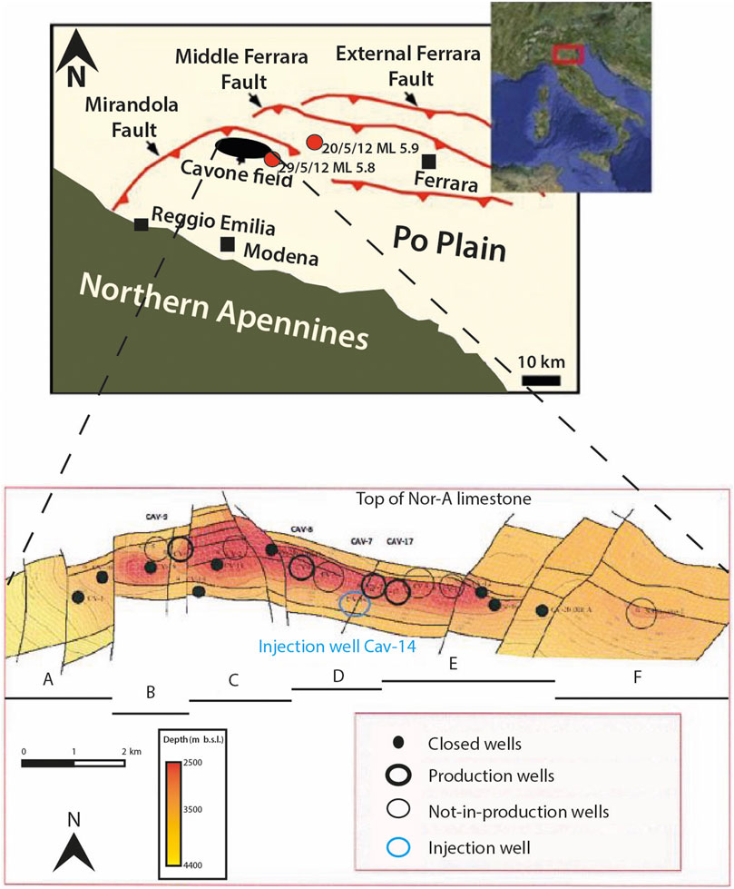
FIGURE 1. Top panel: regional map showing location of the Cavone oil field (the inset highlights the area of interest along the Italian peninsula), epicentral locations of the two 2012 Emilia mainshocks (red circles), and principal thrust faults from Pieri (1983). Bottom panel (Società Padana Energia personal communication, 2019): letters (A–F) indicate the different blocks of the oil field, identified by both the tear faults (have an almost N-S strike) and the topography of the Top of Noriglio-A (Nor-A) formation.
In presenting the 2-year pilot application of the Italian guidelines to the Cavone case, we structure the paper describing the oil field firstly, and then separately outlining the monitoring networks and the specific analysis on microseismicity, ground deformation, and pore pressure data. Finally, we will devote a section to further discussion regarding the tasks assumed by a research institution in monitoring a hydrocarbon deposit. We will highlight strengths and achievements and possible improvements that could be applied both to the general guidelines and their specific implementation, as in the Cavone area of analysis. We aim to contribute to the general discussion on the monitoring of underground energy technologies, drawing from our experience.
2 The Cavone Oil Field
The NE-verging Apennines belt developed during Neogene and Quaternary in the framework of the collision between the European continental margin and the Adria microplate. The fold-and-thrust system is buried by thick Quaternary sediments of the Po plain (Malinverno and Ryan, 1986; Doglioni et al., 1999). The Mirandola anticline belongs to the Ferrara arc (Scrocca et al., 2007; Carminati et al., 2010; Govoni et al., 2014) and is located in the Apennines foreland. In the Mirandola area correspondence, the Apennines belt front has a roughly E-W trending (Pieri, 1983; Burrato et al., 2003; Figure 1). The Cavone oil field is set in correspondence of a “structural high” of the Mirandola anticline. Tectonic structures in this area are dominated by deep-seated reverse faults or blind thrusts (Ciaccio and Chiarabba, 2002). This structural style is evident in the Cavone oilfield area: in this segment the Mirandola thrust (that hosted the 29 May ML 5.8 s main-shock of the 2012 Emilia sequence) has a roughly WE strike, is south dipping, and superimposed by a north-vergent fault-propagation fold (Suppe and Medwedeff, 1990; Carminati and Vadacca, 2010). The main structural lineaments are sketched in the map included in the top panel of the Figure 1. The Cavone oil field is placed 25 km north of Modena (Northern Italy), in the exploitation permit named “Mirandola”. Its area is about 15 km2, and the productive reservoir datum is 2,900 m at depth, mainly hosted inside a carbonatic sequence. The discovering of the oil field happened in 1973 after a deep exploration of the Ferrara arc’s more internal front and the positive feedback obtained by the Cavone1 well. The oil field is segmented by a set of N-S tear faults that divided the anticline, perpendicularly to its strike, in different domains (defined blocks A,B,C,D,E, and F on Figure 1). The fluid extracted from the reservoir is a mixture of oil, methane gas, and water. Two nonproductive wells (Cavone5 e Cavone14) were dedicated to re-injection of the produced waters, even though in practice only the Cavone14 (placed at the boundary between D and E block) is used at this scope since January 1993. The injection is performed at a depth range from 3,302 to 3,367 m, deeper than the “water-oil contact” (3,130 m deep) starting level in the Noriglio-B limestone formation, beneath the Noriglio-A limestone formation (ICHESE, 2014).
3 Seismic Monitoring
The guidelines define two volumes of interest around the reservoir where the monitoring efforts have to be addressed: an Internal Domain (ID) where it is plausible that induced seismicity may occur, and an Extended Domain (ED), surrounding the ID, useful for better contextualisation of the observed seismicity. In the case of hydrocarbon cultivation with re-injection of the produced water inside the reservoir (the Cavone case) the ID is the volume that includes the mineralised zone, reaches the surface, and extends for further 5 km from the border and bottom of the reservoir; while the ED is the volume range that extends from the ID for further 5 km in all directions (Dialuce et al., 2014; see Figure 2).
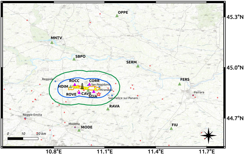
FIGURE 2. Map of the Cavone oil field with local VO seismic stations (purple triangles) and Italian Seismic Network IV station (green triangles) locations. The yellow circles indicate the approximate positions of the extraction wells, while the injection one is sketched in black. The orange line delineates the reservoir projection on the surface. The blue and green lines are contouring the domains of interest ID and ED respectively (see text for more details). The red stars show the locations of the historical earthquakes with MW ≥ 4.5, occurred in the area, with the bigger one highlighting that on the 29 May, 2012, as from Rovida et al. (2020).
The Cavone seismic network in the current configuration has been installed in November, 1990, it consists of four stations, whose name and coordinates are listed in Supplementary Table S1 and mapped in Figure 2 (purple triangles). All stations are equipped with 3-component Lennartz Le-3D/1s sensors, and were firstly coupled with Lennartz MARS88 (Lennartz Electronic GmbH), they were working in triggering mode and synchronised through DCF-77 radio signal until December 18, 2018. Subsequently, the MARS88 have been substituted with Dymas24 by Sara Electronic Instruments S.r.l., which allows a continuous acquisition and a GPS synchronisation, thus reaching the current standard level for a seismic network. To ensure a unique data flux the local network have been registered at the International Federation of the Digital Seismic Networks as VO, with station names CORR, ROCC, ROVE e SGIA that have been registered at the International Registry of Seismograph Stations. The sampling frequency is now (since the network improvement of December 2018) 200 Hz, that allows a signal band of 1–80 Hz. In the guidelines’ experimental period, the local seismic network has been enhanced with the 10 stations of the Italian Seismic Network (network code IV) in a radius of 50 km from San Possidonio (the village with a central location with respect to the reservoir elongation), shown as green triangles in the map of Figure 2 and listed in Supplementary Table S2. INGV manages these latter stations, and all technical information are reported in the network webpage (INGV Seismological Data Centre, 2006). The integrated seismic network includes thus 14 stations, six of them are located close to each other inside the reservoir projection at the surface, one (RAVA) is just outside all detection domains, while the other seven are quite far away.
3.1 Seismic Network Performance Evaluation
Before starting the monitoring phase, we evaluate the seismic network’s theoretical performance in terms of detection threshold, i.e., the minimum magnitude event that has a 90% probability of being identified and accurately localized using the data acquired by the network stations (Ringdal, 1975). For estimating the network detection threshold we followed a mixed indirect approach based on the comparison of the real noise level recorded at the seismic stations with the theoretical spectra associated to the rupture models for small earthquakes (McNamara et al., 2004; Marzorati and Bindi, 2006; Vassallo et al., 2012).
The Cavone oil field area’s noise level, has been evaluated on the basis of 15 days of seismic signal acquired between 1 and 15 September, 2018 at NDIM and CAVE stations. These two IV stations (INGV Seismological Data Centre, 2006), are the closest to the Cavone oil field (a few kilometres away from the reservoir, Figure 2), and are equipped with broad band velocimeters. Unlike the monitoring stations of the local VO network, they were continuously recording at that time. We extended the results of the noise analysis produced for NDIM and CAVE to the local VO seismic stations for the above mentioned reasons, and only afterwards, with the continuous data from the VO stations, we could verify that the seismic noise recordings of all these stations are very similar (see Supplementary Figures S1, S2 for comparison). We analysed the three components continuous recordings for characterising their noise levels in terms of Power Spectral Density (PSD, Peterson, 1993). We computed the PSD on all 1-h segments, sliding half an hour, composing the continuous recording of each station component, thus enhancing the noise sources’ spectral characteristics (Peterson, 1993). Figure 3 shows the spectrograms obtained starting from the PSDs calculated for the two stations. Seismic noise shows a clear day-night variation with noise levels that increase during the day and decrease at night. This characteristic appears clearly at low periods (less than 1 s, see panel c in Figure 3) for both stations at all components. Figure 4 shows the temporal variations of the seismic noise calculated in three different period ranges: 0.07 ÷ 0.15 s; 0.7 ÷ 1.4 s; 7.2 ÷ 14 s. The seismic noise recorded at CAVE at low period (0.07÷0.15 s) decreases by about 20–25 dB during night compared to the daytime levels. Similar variations are also observed for the NDIM station where a decrease in noise levels by about 25–30 dB is observed during the nights for all components. Also in the intermediate period band (0.7÷1.4 s) there is an important but more contained day-night variation compared to the previous band. In effect, in the latter band, the noise level decreases by about 10–15 dB at night for both CAVE and NDIM stations. Finally, at high periods, between 7.2÷14 s, there are no important variations attributable to the day-night transition. Furthermore, the spectrograms and the PSD temporal variations (Figures 3, 4) highlight a decrease of noise level in the two period bands 0.07 ÷ 0.15 s and 0.7÷1.4 s during the weekends (days 1, 2, 8, 9, and 15 of September, 2018). Both the observed day-night variations and the noise decrease during the weekends suggest that anthropogenic noise is among the main source of low period/high frequency noise (periods less than 1.4 s, frequencies higher than 0.7 Hz) recorded at these stations. Through a statistical analysis carried out on all the PSD curves computed for the different hours, we determined the PSD curves relating to the 90-th percentile for each component. These curves were considered as reference levels of towing to the stations to derive the entire network’s detection thresholds. For the local VO network (CORR, ROC, ROVE, SGIA), we adopted the 90-th percentile curves of the CAVE station as representative. This station was chosen as a reference since, similarly to the Cavone oil field stations, it is positioned further away from anthropogenic noise sources compared to NDIM (which is located in the urban area of the municipality of Novi di Modena, Modena province).
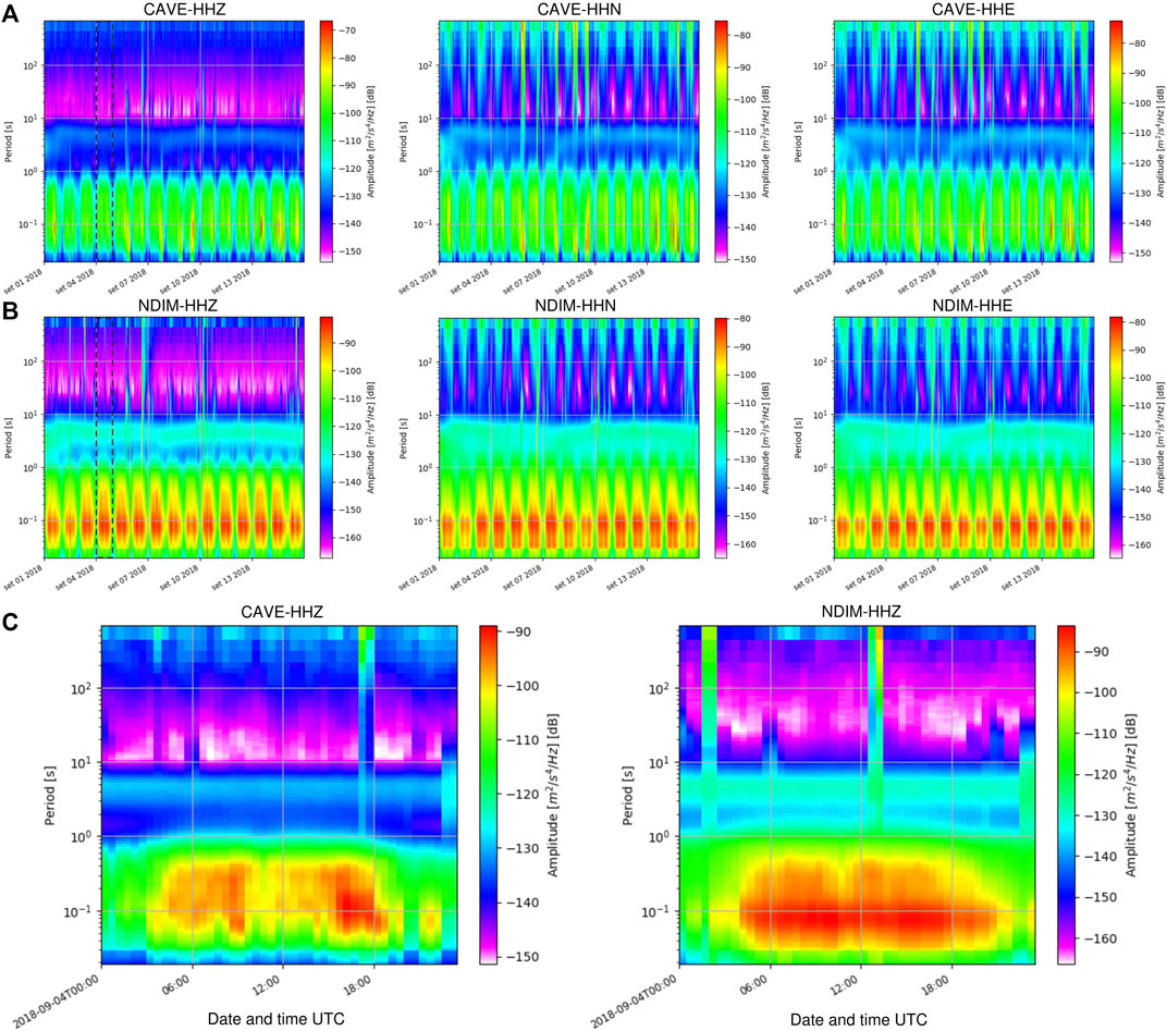
FIGURE 3. Spectrograms for the three components of CAVE (A) and NDIM (B) stations using the data acquired from 1 to 15 September, 2018. In (C) is a zoom on the day of 4 September for both stations vertical components, to emphasise the daytime increase in seismic noise levels at periods less than 1 s. The selected day is indicated by the dashed vertical lines in the HHZ spectrograms of panels (A) and (B). The color scale represents the PSD value in dB with respect to 1 m/s and is optimised for each sub-figure.
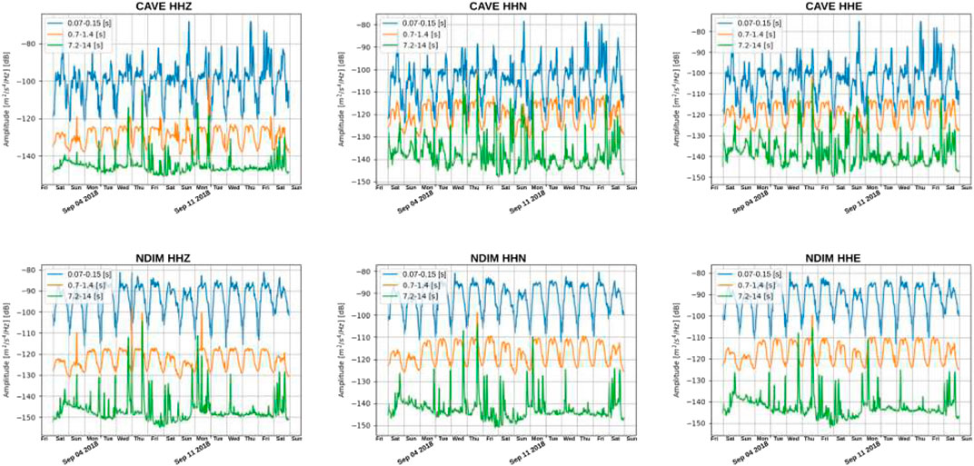
FIGURE 4. Time variability of the noise levels (PSD in dB) averaged in three different period bands (0.07 ÷ 0.15 s; 0.7 ÷ 1.4 s; 7.2 ÷ 14 s) for the three components of CAVE and NDIM stations using the data recorded between 1 and 15 September, 2018. In each sub-plot, the corresponding days of the week are shown on the abscissa axis in order to emphasise the diurnal variations of the noise level and the variations during the weekends.
We used the Brune source model in a homogeneous medium to represent the P and S amplitude spectra of the recorded velocity associated to an earthquake of fixed seismic moment and recorded at a fixed hypocentral distance. The Brune spectrum is computed after defining the seismic source and propagation medium parameters such as stress-drop, density, P and S waves velocities, anelastic attenuation. For the investigated area, we used: stress-drop Δσ = 1.0 MPa, attenuation t* = 0.08 s (reduced time) (Carannante et al., 2020), Vp = 4,400 m/s, Vs = 2,500 m/s, density ρ = 2.4 g/cm3 (Malagnini et al., 2012; Milana et al., 2014). We also need to set the average depth of the seismic events recorded in this area, from the seismicity analysis results reported in the following Section 3.2, we fixed this value to 6 km. In this way, for a single station the P and S waves’ theoretical amplitude depends on the hypocentral distance, i.e., on the earthquake location. To investigate the areal dependence of the source signal, we defined a regular grid with cell size of 1 × 1 km2, then we moved the epicentral location along each node of the grid, by setting its depth at 6 km. For each node, we then computed the smallest amplitude associated with a seismic event recorded by at least five stations with a signal-to-noise ratio higher than 5, and from that amplitude value we could then retrieve the seismic moment that could generate it, i.e., the Mw associated to the smallest detectable event. The 90-th percentile curves in 1–30 Hz band for vertical and horizontals components are used for computing the signal-to-noise ratio and for determining the detection threshold map for P and S waves. The thresholds that were chosen for the signal-to-noise ratio and for the number of stations ensure an accurate estimation of both location and magnitude (Vassallo et al., 2012). Figures 5A,B show the detection thresholds maps determined for the Cavone oil field for P and S waves. The smallest magnitudes detectable at all points inside both ID and ED are 2.1 for P waves and 1.6 for S waves. However, the maps show significant spatial variations of about 0.2–0.3 units in MW which are mainly attributable to the network geometry since for threshold evaluation we used noise levels equals for all the involved stations except for NDIM. Beyond the scientific interest in testing the seismic network’s possible performance, the guidelines (Dialuce et al., 2014) require minimum requisite in terms of seismic network performance. In particular, the seismic network should “in the internal detection domain, detect and locate earthquakes starting from local magnitude ML between 0 and 1 (0 ≤ ML ≤ 1)”. The detection thresholds obtained from the proposed analysis show minimum magnitudes in the ID greater than those required by the guidelines, considering the ML − MW relationship for small earthquakes (Munafò et al., 2016). This may be due either to the high seismic noise present in the Cavone oil field area at high frequency (
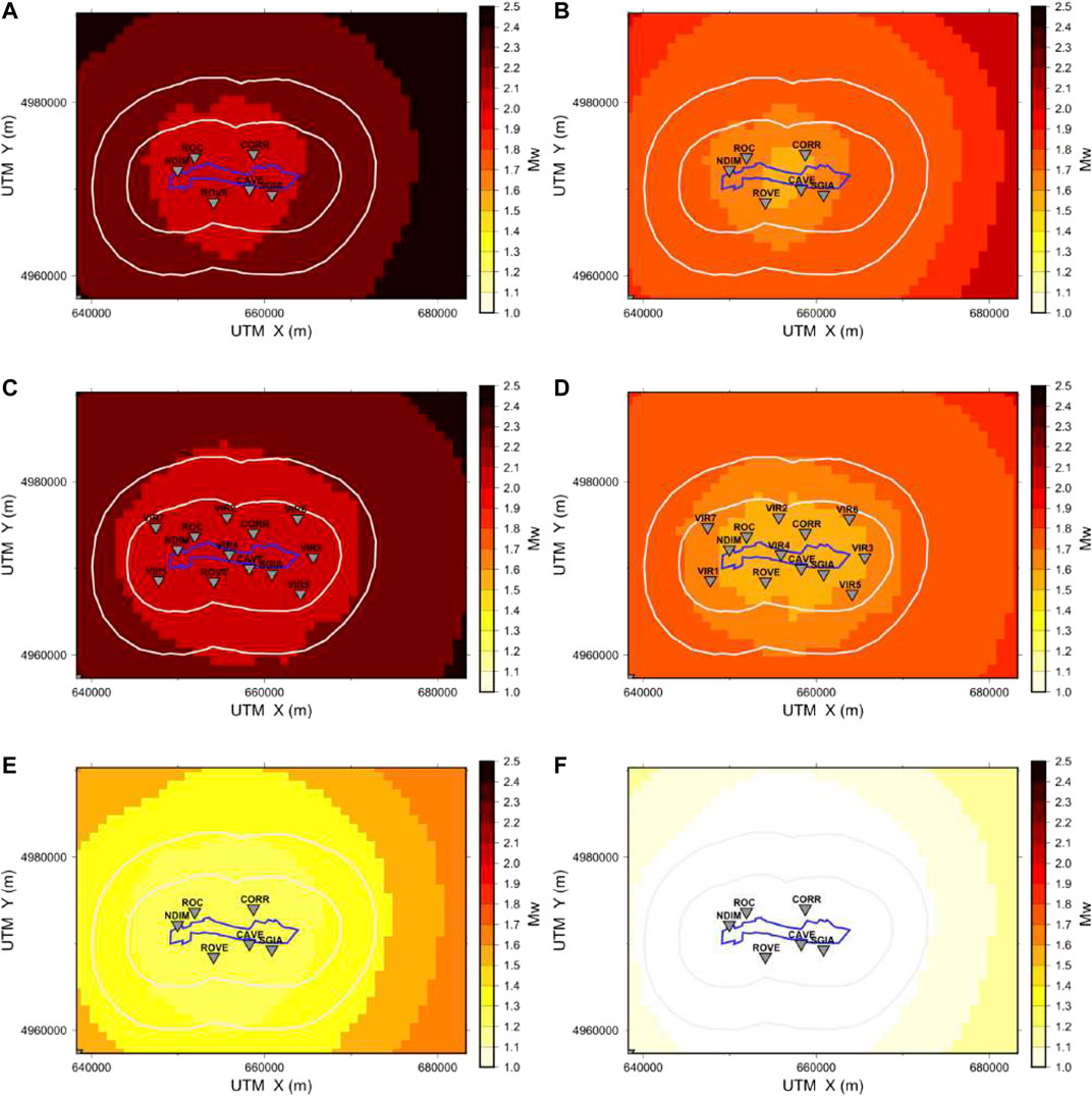
FIGURE 5. Detection threshold maps for the Cavone oil field area for P and S waves (left and right columns respectively). Panels (A) and (B) report the results for the actual network composed by four VO and two IV stations. The detection thresholds in (C) and (D) are computed for the improved network composed by the six actual stations and seven virtual stations (VIR). The maps in (E) and (F) show the detection thresholds obtained assuming the actual six seismic stations as placed in boreholes at a depth of about 120 m, and considering a reduction in PSD levels (in 1–30 Hz range) equal to 25 dB for each station and component.
3.2 Cavone Seismicity
During the 2018–2019 period of guidelines’ experimentation we detected, located and analysed 49 events (listed in Table 1). In the first year the seismic network was operating in triggering mode, therefore this list of events does not constitute a homogeneous catalog (and in fact events falling far away from the reservoir are detected only in 2019, as specified in the following). We could not work in real-time because in the second year we just started setting up the entire monitoring structure (hardware and software), hence the data were transferred by the operator every 3 months and we reported our analysis during the sporadic operational committee meetings. Nevertheless, even without a real-time response to the event detection, we could profit from this experimentation period for setting the basis for hydrocarbon cultivation seismic monitoring, understanding the local background seismicity and the real performances of the integrated seismic networks. After picking the P and S phases we localised each event using the Hypoellipse software by Lahr (1989) and a 1-D model built ad-hoc for the Cavone oil field by the operator and provided to us in the framework of the experimental monitoring (Società Padana Energia, personal communication, 2018; and Supplementary Table S3). We preliminarily performed a comparison for testing the performance of this local velocity model (“Cavone-model”) with respect to the one built by (Govoni et al., 2014) for the 2012 Emilia sequence. We located thousand of earthquakes occurred during the seismic sequence in 2012 in the ID area. The location errors computed with the two different velocity models are reported in the Supplementary Figure S3, and show lower values for the Cavone-model, thus supporting its use in locating the 2018–2019 events. Some of the IV stations demonstrated to be too far away for being sensitive to this kind of low energetic seismicity in a noisy (both in high frequencies due to the human activity, and in the low frequencies due to the superficial soft sediments) alluvial plain: FERS, MNTV, and OPPE stations do not detect any of the events, while FIU only one. Still, the six remaining stations were very helpful in locating this seismicity especially by adding useful picks to those events occurred inside the network, allowing minor RMS, and errors on the locations (see Supplementary Table S4). Although we are aware about the variability of the location procedure, which depends on the input parameters and on the personal choices of the analyst (for time picks definition), and of the epistemic uncertainty (Garcia-Aristizabal et al., 2020), we operate as these locations were reliable enough. This is a first approximation: we leave for a future monitoring period to determine the probabilistic locations able to take into accounts all different sources of uncertainties. More than half out of these 49 events (32, i.e., 65% of the total), fall inside the ID, 10 are located in the ED, and seven are out of both domains (see Figure 6). We observe that the epicenters mainly follow the E-W elongated reservoir projection on the surface, but this may be also an effect of the seismic network configuration with six stations installed well inside the ID or even along the borders of the same reservoir projection (Figure 2). The locations of course suffer by variable error measurements that are reported in the Supplementary Table S4, depending mainly on the number of available picks. Then we computed the moment magnitude MW for all events. In case of small earthquakes (MW < 3, i.e., our case) the MW estimate does not yet rely on a routine procedure due to technical difficulties and the only viable option for the quantification of accurate MW is the spectral correction. Therefore, we followed the technique defined by Munafò et al. (2016): we maximized the signal-to-noise-ratio (SNR) through a procedure based on the analysis of peak values of bandpass-filtered time histories by relying on a tool called Random Vibration Theory (RVT, Cartwright and Longuet-Higgins, 1956). We then computed the seismic moments after spectral correction for the regional attenuation parameters (Malagnini and Munafò, 2017), and calculating the RMS values of the low frequency spectral plateaus on the Fourier amplitudes; on the peak amplitudes we use previous results to compute all moments by spectral ratio. By looping through all events, we obtain averages and standard deviations for the seismic moments of all earthquakes in the data set. Our approach provides the utmost accuracy, the measurement errors on our MW estimates are of the order of 0.05, therefore, in a conservative way, we truncated their values at the first decimal digit.
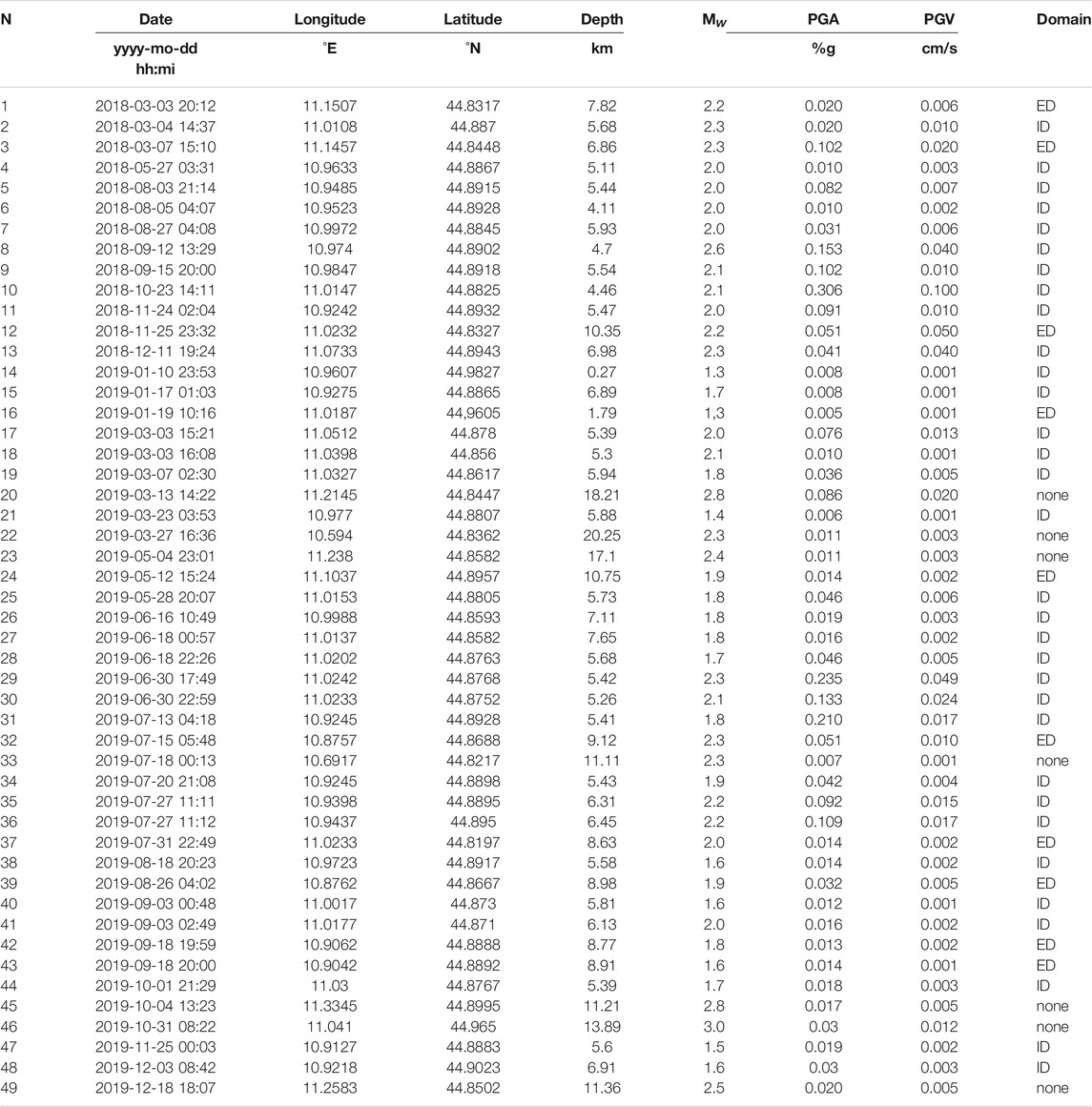
TABLE 1. List of the 49 earthquakes analysed in during 2018–2019. The date is expressed in year-month-day, then we report location estimates (longitude, latitude and depths in km), MW, PGA in g percentages and PGV in cm/s. The last column report the domain where the hypocenter location falls (ID, ED, or none of the two).
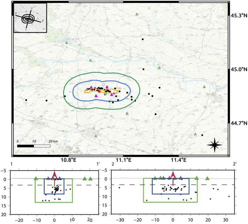
FIGURE 6. Map of the seismicity (black dots) recorded and localised during 2018–2019 monitoring period. The local seismic station (VO network) and Italian Seismic Network station (IV network) locations are also showed as purple and green triangles respectively. The red dot in the map corresponds to the red arrow in the sections below and indicates the position of the Cavone14 injection well. The blue and green contour lines sketch the two internal and extended domains of interest. The yellow polygon shows the reservoir projection at the surface, whose depth is approximately on the dashed line in the two vertical sections, while the solid line marks the topography profile.
Peak Ground Velocity and Acceleration (PGV and PGA respectively) have been computed as the maximum values observed in the recordings (velocity) and their derivatives (acceleration) at any stations and all horizontal components. All these estimates are listed in Table 1. Even though the catalog is undoubtedly too short for statistical analysis, we estimated the completeness magnitude that is required by the guidelines to be less than one in the ID, just to get a rough idea of what we could expect from our data. A plot of the number of events versus magnitude is reported as Supplementary Figure S4, the completeness magnitude results Mc = 2, in agreement with the theoretical estimates reported in Section 3.1.
4 Crustal Deformation Monitoring
Hydrocarbon production activity involving underground extraction, injection or storage of fluids can induce ground displacements, even of considerable entity of the order of centimeter per year (e.g., Vasco et al., 2000; Teatini et al., 2011; Qu et al., 2015; Deng et al., 2020). An appropriate geodetic monitoring system aims to provide information on both the temporal and spatial evolution of ground deformation (Dialuce et al., 2014), highlighting any variations in space and time with respect to a condition not perturbed by the hydrocarbon production activity. For this purpose in the guidelines the deformation monitoring is recommended to be performed using satellite geodetic techniques, acquiring mainly Global Navigation Satellite System (GNSS), and Interferometric Synthetic Aperture Radar (InSAR) measurements of the superficial projection of the survey domains (internal and extended). The two geodetic techniques are complementary (Montuori et al., 2018) since GNSS data allows to obtain a daily (or sub-daily) evolution of the three-components (E, N, Vertical) position of a GNSS station with millimeter precision, while InSAR measurements can provide spatially-dense information of ground displacement along the satellite line of sight (LOS) direction with a temporal sampling spanning from few days to almost a month, depending on the specific satellite sensor used/available.
A time series of ground displacement obtained from a GNSS station contains signals of different nature, deriving from processes acting on different spatial and temporal scales. The linear term (or displacement velocity), for example, describes the rate at which the station moves in the planar components (east and north) and in the vertical component in a given reference system mainly due to tectonic and geodynamic processes, although the vertical rate is much more sensitive to local, non-tectonic processes, than the horizontal ones (e.g., Devoti et al., 2011; Serpelloni et al., 2013). The accuracy and precision of this measurement depends on the quality of the data recorded by the station, the length of the time series analyzed and the presence and amplitude of other seasonal and non-seasonal signals. Seasonal signals, primarily of annual and semi-annual period, mainly come from loading processes acting at continental and regional scales (e.g., surface hydrology, atmospheric loading). Subsurface hydrology, also, may be responsible for non-seasonal or multi-annual ground displacements (e.g., Silverii et al., 2016; Serpelloni et al., 2018). The same deformation signals are recorded also by InSAR measurements whose temporal sampling allows to extract displacement and related rates along the satellite LOS direction. In order to obtain a more complete 3D picture of the spatial and temporal evolution of ground displacements, it is recommended to integrate the two geodetic measurements when long enough records allow to compare them in terms of velocities and displacement time series.
4.1 GNSS Monitoring
The GNSS monitoring infrastructure of the Cavone hydrocarbon concession consists of one GNSS station (CAVO) installed on December 18, 2018, which is equipped by a geodetic-class receiver, for which only Global Positioning System (GPS) observations are available, and a choke-ring type antenna, with an adequate monumentation suitable for geophysical purposes (as indicated in the guidelines), the latter being co-located with a radar corner reflector. It is the only station located above the oil field (Figure 7) and in around 20 km away there are two active GNSS stations, both located to the north, that are: CONC (Concordia sul Secchia) managed by a private company and part of the NetGeo network, and SBPO (San Benedetto Po), part of the INGV RING network. Given the extension of the field (about 15 km) mainly along the EW direction, the current geodetic network requires significant improvements in order to allow the proper monitoring of crustal deformation signals associated with the hydrocarbon cultivation activities at Cavone. Following the indications of the guidelines, in fact, “the local GPS network of permanent precision stations must be installed, appropriately distributed according to the extension and characteristics of the area to be monitored […] it is required that the stations have inter-distances of less than 10–15 km” (Dialuce et al., 2014). Therefore it would be necessary to install at least three additional monitoring sites, two at the east and west edges and one to the south, allowing to accurately measure the local deformation signals both along the NS direction and along the direction of extension of the reservoir.
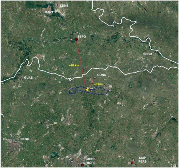
FIGURE 7. Location of the Cavone GNSS station (CAVO) and distance from the nearest active GNSS stations, with the OWC extension projected on the surface shown in blue. Red circles: active RING stations, white circles with names: other active GNSS stations; white circles with no names: other inactive GNSS stations.
During this experimental phase, the available daily raw GPS data, in Receiver INdependent EXchange (RINEX) format of the CAVO station are available form 18 December, 2018 to 31 December, 2019. We have performed a pre-processing step to evaluate the raw observables’ quality by using the TEQC software. The indices considered in this analysis are MP1, i.e., root mean square residual given by multipaths on L1 phase, due to reflections of the radio signal sent by the satellites which affect the correct calculation of the satellite-receiver distance, and MP2, the same as MP1 but for the L2 phase. Supplementary Figure S5 shows the daily MP1 and MP2 values obtained for the CAVO station, and, considering as a reference the IGS network of the International GNSS Service, for which 50% of IGS stations have RMS values for MP1 and MP2 less than 0.4 and 0.6 m respectively, the results indicate that the station records high-quality data.
Subsequently, daily RINEX data have been processed with scientific geodetic software with the aim of estimating the positions of this station in the same, global, international reference frame used for standard INGV processing of the Euro-Mediterranean GNSS stations (e.g., Devoti et al., 2017). We have followed a procedure based on three steps, as described in Serpelloni et al. (2006), Serpelloni et al.(2013), Serpelloni et al.(2018), which consists of: 1) phase analysis, i.e., the observations recorded by the GPS stations of a sub-network that includes CAVO plus other active permanent GPS stations belonging to the EUREF and IGS network (later used to combine the solutions of this sub-network with those of the other sub-networks elaborated at INGV and to align the solutions to a global international reference frame) producing weakly constrained network solutions (positions, orbits, etc…); 2) combination of the daily solutions of the sub-network with the solutions of other subnets processed at INGV and simultaneous alignment of the solutions to the IGS14 reference frame that is the GPS realization of the ITRF2014 reference system (Altamimi et al., 2016); 3) analysis of the time series for the estimation of displacement rates, seasonal signals and uncertainties. For the first two steps, we have used the GAMIT/GLOBK software (version 10.70) obtaining the three-dimensional daily positions and uncertainties for all the stations considered.
The position time series have been analysed in the third step for estimating the linear term of displacement rate in the three components, east, north ,and vertical, by using the analyze_tseri module of the QOCA software. Due to the short time-span available, we do not estimate the seasonal terms. It is worth to note that the scientific literature agrees in defining in 2.5 years the minimum length of a GPS time series for a velocity estimate not influenced by seasonal signals (Blewitt and Lavallée, 2002), and since GNSS time series can be influenced by several other transient signals of tectonic and non-tectonic nature (e.g., Serpelloni et al., 2018), even longer time series may be required (e.g., Masson et al., 2019). Figure 8 shows the displacement time series (with respect to the coordinates calculated at first epoch) of the CAVO station in the east, north and vertical directions, in the IGS14 reference frame. Although the time interval (∼ 1 year) does not allow an evaluation of the seasonal components and an accurate estimate of the displacement rate in the three directions, the data continuity and the low level of noise (NRMS values
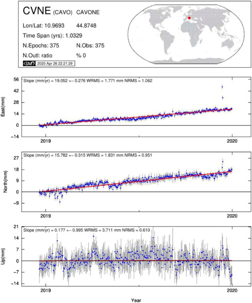
FIGURE 8. Displacement time series of the CAVO station in the IGS14 global reference frame. The gray lines indicate the error bars (1σ) and the red line represents the estimated linear trend.
4.2 InSar Data Analysis
The guidelines for hydrocarbon cultivation activity’s monitoring in the remote sensing domain recommend the use of Synthetic Aperture Radar Interferometry (InSAR) data in a time window of at least 10 years. In this first attempt, we exploit SAR acquisitions from Sentinel-1 mission of the European Space Agency (ESA) since they are free and easily accessible. Moreover, they offer an unprecedented revisit time of 6 days which is an essential condition for the future performing of a quasi-real-time InSAR-based monitoring service. However, the first satellite, i.e., Sentinel-1 A, was launched in 2014 thus reducing the temporal window available for the analysis. In particular, the SAR dataset exploited here consists of 103 images acquired along descending orbit from March 2015 to July 2018. The geometry of view is characterised by incidence and azimuth angle of about 39° and 14°. InSAR analysis was performed by Interferometric Point Target Analysis (IPTA, Werner et al., 2003). We first multi-looked the data by 24 looks along range and six looks along azimuth obtaining a pixel spacing of about 90 m, the same size of the Digital Elevation Model (DEM) of the SRTM mission exploited for removing the topographic contribution in the phase signal. We estimated the interferometric pairs by setting the perpendicular and temporal baseline thresholds to 200 m e 90 days, respectively, obtaining a well connected network of 757 interferograms. We then filtered (Goldstein and Werner, 1998) and unwrapped (Costantini, 1998) all the interferograms and retrieved the InSAR time series by Singular Value Decomposition (SVD) analysis. The results of InSAR analysis in terms of ground velocity are shown in Figure 9. In the Mirandola hydrocarbon cultivation area (the red polygon in the figure), there are no significant deformation patterns associated with the Cavone oil field. Some subsidence phenomena are observed SW the concession area with values peaking at about 2.5 mm/yr. They are probably due to local water pumping activity not connected with the Cavone industrial activity. Such outcome is also shown by InSAR time series extracted from point targets in the proximity of some wells of Cavone field highlighted in Figure 10, top panel. Indeed, quite scattered behaviours are observed along the time series, likely due to seasonal effects or tropospheric artefacts (Figure 10). However, the linear trend along the analysed time window is very close to zero further confirming the absence of any ground deformation phenomena associated with the extraction activity. In conclusion, for the analysed time interval spanning from 2015 to 2018, ground deformations induced by the activity of the Cavone field, detectable within the limit of accuracy of the technique (Casu et al., 2006) are not taking place.
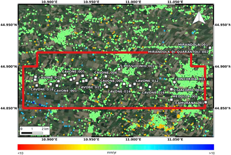
FIGURE 9. Sentinel-1 InSAR Line-of-Sight (LoS) velocity map. The red polygon represents the Mirandola concession area as it was in 2018–2019. The white squares indicate the oil wells.
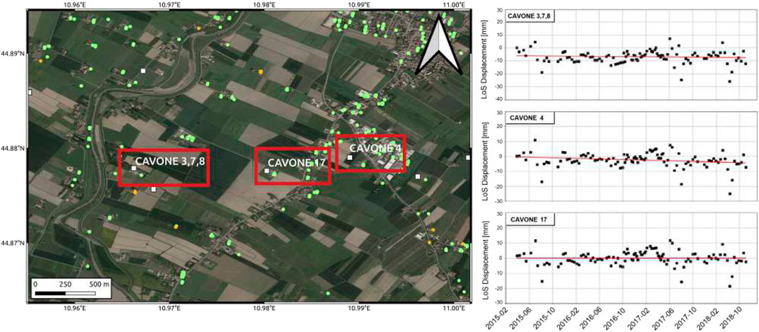
FIGURE 10. Focus on some wells of the Cavone oil field: InSAR time series extracted from point targets in proximity of the wells shown on top.
5 Pore Pressure Monitoring
One of the main interests in seismically monitoring underground industrial activities is understanding whether stress perturbations caused by such activities influence the local seismicity. Nevertheless, discriminating natural from induced seismicity in seismically active regions is a particularly complex task. Early attempts to discriminate induced from natural seismicity were performed, for fluid injection operations, by Davis and Frohlich (1993), and for fluid withdrawal by Davis and Nyffenegger (1995); however, these approaches were mainly based on qualitative assessments. More quantitative approaches, based on physical and/or stochastic features of recorded seismicity also have been proposed in literature (a review can be found, e.g., in Dahm et al., 2015; Schoenball et al., 2015; Grigoli et al., 2017; Garcia et al., 2021). In principle, evaluating possible interactions between seismicity and hydrocarbon production should rely on multidisciplinary analyses such as detailed physically-based modelling and stochastic methods. These latter may provide probabilistic assessments and take uncertainties into account (Segall, 1989; Segall et al., 1994; Gishig and Wiemer, 2013; Dahm et al., 2015; Schoenball et al., 2015; Grigoli et al., 2017; Garcia-Aristizabal, 2018, among others). Even though, the ways in which the interactions may occur are complex, and their identification in a context characterised by naturally-occurring seismicity is not straightforward (Garcia et al., 2021). These reasons stimulate the implementation of alternative statistical methods to track measurable phenomena, as changes in seismicity rates. That rate variations could occur if notable interactions between underground human operations and nearby seismicity sources arise in a given area. In fact, spatial and temporal correlation between human activity and event rates are usually considered key parameters to suspect possible relationships between seismicity and underground anthropic activity (e.g., Shapiro et al., 2007; Cesca et al., 2014; Leptokaropoulos et al., 2017; McClure et al., 2017; Garcia-Aristizabal, 2018; Schultz and Telesca, 2018; Skoumal et al., 2018; Molina et al., 2020).
Among the duties prescribed by the Italian guidelines for geophysical monitoring of underground operations, analyses of the temporal evolution of seismicity, deformation and pore pressure are expected aiming at spotting any possible causal relationships between the industrial activity and the natural observations (Dialuce et al., 2014). With this scope. The daily measurements of the well head pressure were transmitted directly by the operator together with the information on daily volumes of the extracted oil, extracted water, and injected water. Analysing the deformation time series we were unable to discriminate any significant temporal variation (mainly due to the short time span of the data, see section 4). Moreover, considering the limited duration of the experimentation and the relatively low level of seismic activity observed in this area, statistical analyses of possible seismicity rate changes are particularly challenging because of the low number of recorded events. The production in the oil center are carried out at a reasonably constant rate, in particular for the 2018–2019 testing period, apart from a shutdown of the entire plant due to routine maintenance from 16 July to 16 November, 2018. This feature can be seen in Figure 11, where the daily oil and water volumes produced from this field (Figure 11A) and the daily volume and pressure of re-injected water into the Cavone14 well (Figure 11B) present a roughly constant trend, interrupted by the industrial activity stop mentioned before. Figure 12 shows the temporal occurrence of 32 events recorded and located within the internal monitoring domain, plotted against the MW magnitudes (12a), with the shadowed area indicating the shutdown period for reference. Considering the completeness magnitude determined for the MW in this data set (Mc = 2.0), only 10 events above Mc are identified (red circled asterisks in Figure 12). Such a low number of seismic events in the complete catalog makes the statistical analysis application a particularly challenging task that may produce not informative results. For this reason, in this work we only set up a possible analysis procedure to check for possible significant changes in seismicity rates correlated with changes in the industrial activity (i.e., before and after the shutdown period occurred during 4 months in 2018). To perform this task we implement the binomial test (e.g., Wonnacott and Wonnacott, 1977) proposed by Leptokaropoulos et al. (2017), because it is suitable also for few samples. For completeness we show the details of its application on our data in the Supplementary Section 1.
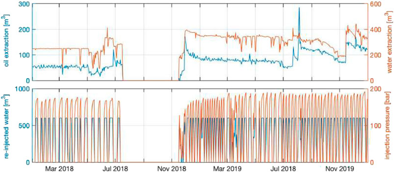
FIGURE 11. (A) Time series of oil and water produced form the Cavone field (m3/day). (B) volume (in m3/day) and pressure (bar) of produced water re-injected through the Cavone14 well.
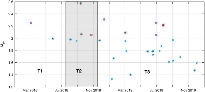
FIGURE 12. Temporal occurrence of the 32 events recorded and located within the internal monitoring domain versus magnitudes MW. The red circles indicate the 10 events for which MW overcomes the completeness magnitude. The shadowed area indicates the industrial activity shutdown period, and the time periods T1, T2, and T3, defined for testing the seismic rate variations are indicated at the bottom.
6 Discussion
The seismic monitoring operated during these 2 years period in the Cavone oil field allowed us to detect and locate 49 events mainly clustered along the reservoir projection on the surface. Nevertheless, the location distribution may be biased by the geometry of the seismic stations (see discussion in Sections 3.1,3.2 and the maps of Figures 2, 6). Even though this seismic catalog is not statistically highly populated, we attempted to estimate the completeness magnitude, finding a value of MW = 2 compatible with the theoretical estimates based on the typical seismic noise recorded at two seismic stations centrally located within the network. This completeness magnitude value would not be in agreement with the guidelines’ requirements, which prescribe the detection and location of events with magnitude less than 1. Possible reasons for such a high value could be ascribed primarily to the high seismic noise of this area due to the resonance of the Po plain sediments, and only secondarily to the seismic network configuration since there are no stations in the ED. From our simulations, in fact, we could show how the main factor in decreasing the detection threshold seems to be the removal of the sedimentary basin resonances by installing borehole stations (as from results in Figure 5). While an even large increase in seismic station number on the surface would not change much the detection threshold, helping only in extending the detection area. This result is not so surprising if we think that the Po plain sedimentary layer may deepen some km from the surface (8.5 km at most, Pieri, 1983). This unfavourable geological condition coupled with a multitude of anthropogenic noise sources (the Po plain is the area with the highest concentration of inhabitants and economic activities in Italy) cause very high seismic noise levels observed thorough the plain (Margheriti et al., 2000; Cocco et al., 2001; Pesaresi et al., 2014; Laurenzano et al., 2017). And the presence of seismic noise generates a low number of detected events and a high completeness magnitude. Anyway, we would need a much longer monitoring period for collecting many more events, necessary to find a stable and reliable value of completeness magnitude. This information would also help in determining the magnitude threshold for passing the color code in the traffic light system (e.g., Bommer et al., 2006) tuned for this specific oil field. The deformation monitoring (mainly from InSAR analysis) did not highilght any significant trend on the surface displacements that may be related to the Cavone industrial activity. We highlight that 1 year of data is too few for a correct GPS analysis. Furthermore, the only GNSS station installed in the area is not enough to thoroughly monitor the possible deformations due to the industrial activities. Even though the Cavone reservoir is surrounded by carbonatic rocks, we strongly recommend as a best practice for this type of study, to implement a monitoring network capable of recording the entire deformation field due to the hydrocarbon production activity, which usually generates the maximum of the vertical displacements at the center of the reservoir, and the maximum of the horizontal ones at the edges. For these reasons in this case we suggest the installation of three more stations (with the same technical characteristics as the one already installed) to the east, west, and south of the reservoir allowing to identify the main surface deformation patterns along the three displacement components.
7 Conclusion
In this paper we report the main outcomes of a 2-year pilot application of the Italian guidelines for monitoring seismicity, ground deformation, and pore pressure in the Cavone hydrocarbon cultivation field, in Northern Italy. We acknowledge that this experiment has been limited in scope by the too-short time period and by the weakness of the geophysical instrument network. In fact, in the monitoring domain only four seismic stations run by the industrial operator, integrated with three stations from INGV’s national network (all located in the highly anthropised and noisy Po plain sedimentary basin) and 1 GNSS receiver station are available for the analysis. In spite of these limitations, helpful considerations may be drawn. The first evident conclusion is that a more extended observation period is needed for a better assessment. In fact the Cavone oil field lies in a seismic territory, but we could not ascertain the background microseismic activity for lack of a detailed survey preceding the oil extraction. Beside, we notice that, given the high natural seismic noise of the environment (Po plain sediments), the magnitude of detection is relatively high compared to the standpoint of the national-scale seismic network, despite the presence of local VO stations in the area. This fact lead us to stress the importance of a seismic monitoring network installed and maintained both before and during extraction and production water re-injection activities. Also, it should consist of borehole installations to reduce the seismic resonance of the plain soft sediments and, consequently, improve the detection capability. All these strategies will extend the magnitude threshold to (much) less energetic seismic events, reaching a crucial point also highlighted by the guidelines. We note also that the operational application of a traffic light system (e.g., Bommer et al., 2006) would require detection of lower-magnitude seismic events. Ground deformation monitoring would also require more than one GNSS station in the area, and a longer observation time. With these limitations, no significant crustal deformation was observed. The seismic events we detected and located are too few for being meaningful on possible significant contribution from the produced water injection on the crustal stress field. However an explicit fluid-geo-mechanical study (outside the scope of the test application of the national guidelines, and of this paper) would be necessary to quantify this effect. Studies of perturbations of the crustal stress field may be particularly important in tectonically active regions, where critically stressed faults are present. A study of this type in the region has been performed by Juanes et al. (2016), who modeled geomechanics and coupled flows for resolving stresses inside and outside the reservoir, assessing the impact of both pressure and effective stress changes on the Mirandola fault. Their results indicate very small stress changes in the region near the May 29, 2012 hypocenter, which drive the authors to conclude that the very minor -if any- effects of production and injection calculated at the hypocenter area may indicate that the combined effects of fluid production and injection from the Cavone oil field were not a driver for the seismicity observed in 2012. To perform a similar modelling, but applied to the microseismicity recorded during this experimental period, a more detailed set of fault planes in and around the reservoir would be required. Therefore a complete 3D maps of the local fault system would be desirable for better understanding the nature of the seismic occurrences.
Data Availability Statement
The data analyzed in this study is subject to the following licenses/restrictions: The Cavone seismic and GNSS network are subject to the third party restrictions: Data are available from the authors with the permission of Società Padana Energia S. p.a. Requests to access these datasets should be directed to TWFzc2ltb0NhcGVsbGV0dGlAZ2FzcGx1cy5pdA==.
Author Contributions
LZ summarised the results in the present paper, co-ordinated the research and monitoring activities, and managed the agreement with the San Possidonio municipality. MA provided the geological information and has performed the P and S phase pickings for the seismic events, and has located them. MV analysed the seismic network detection capability. IMu evaluated the moment magnitude for all seismic events. LF computed the PGA and PGV values. LS estimated the completeness magnitude for the seismic event catalog. AG statistically tested the relationship between seismic rate and industrial activity in time. MP and GP analysed the InSAR data. ES and LA analysed the GPS data. ME produced the maps of the Cavone oil field. IMo and GZ computed and produced the maps for the PPSD at the local VO stations. AM supervised the Cavone experimental application of the guidelines for monitoring industrial activities. All authors participated in writing this article.
Funding
This research was financed by the “Convenzione tra il comune di San Possidonio e l’Istituto Nazionale di Geofisica e Vulcanologia -I.N.G.V.- per l’attuazione del monitoraggio nella concessione di coltivazione idrocarburi “Mirandola” finalizzata alla messa in opera di attività di monitoraggio di sperimentazione degli indirizzi e linee guida per i monitoraggi ILG ed assunzione funzioni di Struttura Preposta al Monitoraggio di cui all’art. 6 del Protocollo Operativo”.
Conflict of Interest
The authors declare that the research was conducted in the absence of any commercial or financial relationships that could be construed as a potential conflict of interest.
Publisher’s Note
All claims expressed in this article are solely those of the authors and do not necessarily represent those of their affiliated organizations, or those of the publisher, the editors and the reviewers. Any product that may be evaluated in this article, or claim that may be made by its manufacturer, is not guaranteed or endorsed by the publisher.
Acknowledgments
We thank the MiSE and Società Padana Energia S.p.a. staff, in particular M. Capelletti and C. Triunfo for the fruitful collaboration. We profit by the discussion with L. Martelli, D. Susanni, and M. Mileti, and more generally all participants to the operational committee meetings. We thank Leica-Geosystem and Topcon Positioning Italy for providing GPS data of the SmartNet and NetGeo GNSS networks, respectively, and the European Space Agency for providing Sentinel-1 SAR data. We greatly thank two reviewers that helped us in deeply improving the article.
Supplementary Material
The Supplementary Material for this article can be found online at: https://www.frontiersin.org/articles/10.3389/feart.2021.685300/full#supplementary-material
References
Altamimi, Z., Rebischung, P., Métivier, L., and Collilieux, X. (2016). ITRF2014: A New Release of the International Terrestrial Reference Frame Modeling Nonlinear Station Motions. J. Geophys. Res. Solid Earth 121, 6109–6131. doi:10.1002/2016jb013098
Blewitt, G., and Lavallée, D. (2002). Effect of Annual Signals on Geodetic Velocity. J. Geophys. Res. 107, B7. doi:10.1029/2001jb000570
Bommer, J. J., Oates, S., Cepeda, J. M., Lindholm, C., Bird, J., Torres, R., et al. (2006). Control of hazard Due to Seismicity Induced by a Hot Fractured Rock Geothermal Project. Eng. Geol. 83, 287–306. doi:10.1016/j.enggeo.2005.11.002
Braun, T., Danesi, S., and Morelli, A. (2020). Application of Monitoring Guidelines to Induced Seismicity in italy. J. Seismol. 24, 1015–1028. doi:10.1007/s10950-019-09901-7
Carannante, S., D’Alema, E., Augliera, P., and Franceschina, G. (2020). Improvement of Microseismic Monitoring at the Gas Storage Concession “Minerbio Stoccaggio” (Bologna, Northern Italy). J. Seismol. 24, 967–977. doi:10.1007/s10950-019-09879-2
Carminati, E., Scrocca, D., and Doglioni, C. (2010). Compaction-induced Stress Variations with Depth in an Active Anticline: Northern Apennines, Italy. J. Geophys. Res. 115, 17p. doi:10.1029/2009JB006395
Carminati, E., and Vadacca, L. (2010). Two- and Three-Dimensional Numerical Simulations of the Stress Field at the Thrust Front of the Northern Apennines, Italy. J. Geophys. Res. 115, 21p. doi:10.1029/2010JB007870
Cartwright, D. E., and Longuet-Higgins, M. S. (1956). The Statistical Distribution of the Maxima of a Random Function. Proc. Math. Phys. Sci. 237, 212–232.
Casu, F., Manzo, M., and Lanari, R. (2006). A Quantitative Assessment of the Sbas Algorithm Performance for Surface Deformation Retrieval from Dinsar Data. Remote Sensing Environ. 102, 195–210. doi:10.1016/j.rse.2006.01.023
Cesca, S., Braun, T., Maccaferri, F., Passarelli, L., Rivalta, E., and Dahm, T. (2013). Source Modelling of the M5-6 Emilia-Romagna, Italy, Earthquakes (2012 May 20-29). Geophys. J. Int. 193, 1658–1672. doi:10.1093/gji/ggt069
Cesca, S., Grigoli, F., Heimann, S., González, Á., Buforn, E., Maghsoudi, S., et al. (2014). The 2013 September-October Seismic Sequence Offshore Spain: a Case of Seismicity Triggered by Gas Injection? Geophys. J. Int. 198, 941–953. doi:10.1093/gji/ggu172
Ciaccio, M. G., and Chiarabba, C. (2002). Tomographic Models and Seismotectonics of the Reggio Emilia Region, Italy. Tectonophysics 344, 261–276. doi:10.1016/S0040-1951(01)00275-X
Cocco, M., Ardizzoni, F., Azzara, R. M., Dall’Olio, L., Delladio, A., Di Bona, M., et al. (2001). Broadband Waveforms and Site Effects at a Borehole Seismometer in the Po Alluvial basin (Italy). Ann. Geophys. 44, 137–154. doi:10.4401/ag-3611
Costantini, M. (1998). A Novel Phase Unwrapping Method Based on Network Programming. IEEE Trans. Geosci. Remote Sensing 36, 813–821. doi:10.1109/36.673674
Dahm, T., Cesca, S., Hainzl, S., Braun, T., and Krüger, F. (2015). Discrimination between Induced, Triggered, and Natural Earthquakes Close to Hydrocarbon Reservoirs: A Probabilistic Approach Based on the Modeling of Depletion-Induced Stress Changes and Seismological Source Parameters. J. Geophys. Res. Solid Earth 120, 2491–2509. doi:10.1002/2014jb011778
Davis, S. D., and Frohlich, C. (1993). Did (Or Will) Fluid Injection Cause Earthquakes? - Criteria for a Rational Assessment. Seismol. Res. Lett. 64, 207–224. doi:10.1785/gssrl.64.3-4.207
Davis, S. D., and Nyffenegger, P. A. (1995). The 9 April 1993 Earthquake in South-central Texas: Was it Induced by Fluid Withdrawal? Bull. Seismol. Soc. Am. 85, 1888–1895.
Deng, F., Dixon, T. H., and Xie, S. (2020). Surface Deformation and Induced Seismicity Due to Fluid Injection and Oil and Gas Extraction in Western Texas. J. Geophys. Res. Solid Earth 125, e2019JB018962. doi:10.1029/2019JB018962
Devoti, R., D'Agostino, N., Serpelloni, E., Pietrantonio, G., Riguzzi, F., Avallone, A., et al. (2017). A Combined Velocity Field of the Mediterranean Region. Ann. Geophys. 60, 0215. doi:10.4401/ag-7059
Devoti, R., Esposito, A., Pietrantonio, G., Pisani, A. R., and Riguzzi, F. (2011). Evidence of Large Scale Deformation Patterns from GPS Data in the Italian Subduction Boundary. Earth Planet. Sci. Lett. 311, 230–241. doi:10.1016/j.epsl.2011.09.034
Dialuce, G., Chiarabba, C., Bucci, D. D., Doglioni, C., Gasparini, P., Lanari, R., et al. (2014). Indirizzi e linee guida per il monitoraggio della sismicità, delle deformazioni del suolo e delle pressioni di poro nell’ambito delle attività antropiche. Available at: https://unmig.mise.gov.it/images/docs/151_238.pdf (Last Accessed November 04, 2021).
Doglioni, C., Harabaglia, P., Merlini, S., Mongelli, F., Peccerillo, A., and Piromallo, C. (1999). Orogens and Slabs vs. Their Direction of Subduction. Earth Sci. Rev. 45, 167–208. doi:10.1016/s0012-8252(98)00045-2
Enrico Serpelloni, E., Marco Anzidei, M., Paolo Baldi, P., Giuseppe Casula, G., and Alessandro Galvani, A. (2012). GPS Measurement of Active Strains across the Apennines. Ann. Geophys. 49, 319–329. doi:10.4401/ag-5756
Garcia, A., Faenza, L., Morelli, A., and Antoncecchi, I. (2021). Can Hydrocarbon Extraction From the Crust Enhance or Inhibit Seismicity in Tectonically Active Regions? A Statistical Study in Italy. Front. Earth Sci. 9:673124. doi:10.3389/feart.2021.673124
Garcia-Aristizabal, A., Danesi, S., Braun, T., Anselmi, M., Zaccarelli, L., Famiani, D., et al. (2020). Epistemic Uncertainties in Local Earthquake Locations and Implications for Managing Induced Seismicity. Bull. Seismol. Soc. Am. 110, 2423–2440. doi:10.1785/0120200100
Garcia-Aristizabal, A. (2018). Modelling Fluid-Induced Seismicity Rates Associated with Fluid Injections: Examples Related to Fracture Stimulations in Geothermal Areas. Geophys. J. Int. 215, 471–493. doi:10.1093/gji/ggy284
Garofalo, F., Foti, S., Hollender, F., Bard, P. Y., Cornou, C., Cox, B. R., et al. (2016). InterPACIFIC Project: Comparison of Invasive and Non-invasive Methods for Seismic Site Characterization. Part II: Inter-comparison between Surface-Wave and Borehole Methods. Soil Dyn. Earthquake Eng. 82, 241–254. doi:10.1016/j.soildyn.2015.12.009
Gishig, V., and Wiemer, S. (2013). A Stochastic Model for Induced Seismicity Based on Nonlinear Pressure Diffusion and Irreversible Permeability Enhancement. Geophys. J. Int. 194, 1229–1249. doi:10.1093/gji/ggt164
Goldstein, R. M., and Werner, C. L. (1998). Radar Interferogram Filtering for Geophysical Applications. Geophys. Res. Lett. 25, 4035–4038. doi:10.1029/1998GL900033
Govoni, A., Marchetti, A., De Gori, P., Di Bona, M., Lucente, F. P., Improta, L., et al. (2014). The 2012 Emilia Seismic Sequence (Northern Italy): Imaging the Thrust Fault System by Accurate Aftershock Location. Tectonophysics 622, 44–55. doi:10.1016/j.tecto.2014.02.013
Grigoli, F., Cesca, S., Priolo, E., Rinaldi, A. P., Clinton, J. F., Stabile, T. A., et al. (2017). Current Challenges in Monitoring, Discrimination, and Management of Induced Seismicity Related to Underground Industrial Activities: A European Perspective. Rev. Geophys. 55, 310–340. doi:10.1002/2016RG000542
ICHESE (2014). Report on the Hydrocarbon Exploration and Seismicity in Emilia Region. Paper Presented at International Commission on Hydrocarbon Exploration and Seismicity in the Emilia Region. Available at: http://mappegis.regione.emilia-romagna.it/gstatico/documenti/ICHESE/ICHESE_Report.pdf.
INGV Seismological Data Centre (2006). Rete Sismica Nazionale. Italy: Istituto Nazionale di Geofisica e Vulcanologia (INGV). doi:10.13127/SD/X0FXNH7QFY
Juanes, R., Jha, B., Hager, B. H., Shaw, J. H., Plesch, A., Astiz, L., et al. (2016). Were the May 2012 Emilia-Romagna Earthquakes Induced? a Coupled Flow-Geomechanics Modeling Assessment. Geophys. Res. Lett. 43, 6891–6897. doi:10.1002/2016gl069284
Keranen, K. M., Savage, H. M., Abers, G. A., and Cochran, E. S. (2013). Potentially Induced Earthquakes in oklahoma, usa: Links between Wastewater Injection and the 2011 Mw 5.7 Earthquake Sequence. Geology 41, 699–702. doi:10.1130/g34045.1
Lahr, J. C. (1989). Hypoellipse/version 2.0: A Computer Program for Determining Local Earthquake Hydrocentral Parameters, Magnitude, and First Motion Pattern: Open-File Report. Menlo Park, California: U.S. Geological Survey, 89–116. doi:10.3133/ofr89116
Laurenzano, G., Priolo, E., Mucciarelli, M., Martelli, L., and Romanelli, M. (2017). Site Response Estimation at Mirandola by Virtual Reference Station. Bull. Earthquake Eng. 15, 2393–2409. doi:10.1007/s10518-016-0037-y
Leptokaropoulos, K., Staszek, M., Lasocki, S., Martínez-Garzón, P., and Kwiatek, G. (2017). Evolution of Seismicity in Relation to Fluid Injection in the North-Western Part of the Geysers Geothermal Field. Geophys. J. Int. 212, 1157–1166. doi:10.1093/gji/ggx481
Luca Minarelli, L., Sara Amoroso, S., Gabriele Tarabusi, G., Marco Stefani, M., and Gabriele Pulelli, G. (2016). Down-hole Geophysical Characterization of Middle-Upper Quaternary Sequences in the Apennine Foredeep, Mirabello, Italy. Ann. Geophys. 59, S0543. doi:10.4401/ag-7114
Maesano, F. E., D'Ambrogi, C., Burrato, P., and Toscani, G. (2015). Slip-rates of Blind Thrusts in Slow Deforming Areas: Examples from the Po Plain (Italy). Tectonophysics 643, 8–25. doi:10.1016/j.tecto.2014.12.007
Malagnini, L., Herrmann, R. B., Munafò, I., Buttinelli, M., Anselmi, M., Akinci, A., et al. (2012). The 2012 Ferrara Seismic Sequence: Regional Crustal Structure, Earthquake Sources, and Seismic hazard. Geophys. Res. Lett. 39, a–n. doi:10.1029/2012GL053214
Malagnini, L., and Munafò, I. (2017). Mws of Seismic Sources under Thick Sediments. Bull. Seismol. Soc. Am. 107, 1413–1420. doi:10.1785/0120160243
Malinverno, A., and Ryan, W. B. F. (1986). Extension in the Tyrrhenian Sea and Shortening in the Apennines as Result of Arc Migration Driven by Sinking of the Lithosphere. Tectonics 5, 227–245. doi:10.1029/TC005i002p00227
Margheriti, L., Azzara, R. M., Cocco, M., Delladio, A., and Nardi, A. (2000). Analysis of Borehole Broadband Recordings: Test Site in the Po Basin, Northern Italy. Bull. Seismol. Soc. Am. 90, 1454–1463. doi:10.1785/01199900616
Martelli, L., Calabrese, L., Ercolessi, G., Molinari, F. C., Severi, P., Bonini, M., et al. (2017). “The New Seismotectonic Map of the Emilia-Romagna Region and Surrounding Areas,” in Atti Del. 36° Convegno Nazionale GNTS, Trieste, Italy, November 14–16, 2017, 47–53.
Marzorati, S., and Bindi, D. (2006). Ambient Noise Levels in north central italy. Geochem. Geophys. Geosyst. 7, Q09010. doi:10.1029/2006GC001256
Masson, C., Mazzotti, S., Vernant, P., and Doerflinger, E. (2019). Extracting Small Deformation beyond Individual Station Precision from Dense Global Navigation Satellite System (GNSS) Networks in France and Western Europe. Solid Earth 10, 1905–1920. doi:10.5194/se-10-1905-2019
Maury, V. M. R., Grassob, J.-R., and Wittlinger, G. (1992). Monitoring of Subsidence and Induced Seismicity in the Lacq Gas Field (france): the Consequences on Gas Production and Field Operation. Eng. Geol. 32, 123–135. doi:10.1016/0013-7952(92)90041-v
McClure, M., Gibson, R., Chiu, K. K., and Ranganath, R. (2017). Identifying Potentially Induced Seismicity and Assessing Statistical Significance in oklahoma and california. J. Geophys. Res. 122, 2153–2172. doi:10.1002/2016jb013711
McNamara, D. P. B. R., Buland, R. P., Benz, H., and Leith, W. (2004). Earthquake Detection and Location Capabilities of the Advanced National Seismic System. American Geophysical Union, Fall Meeting, San Francisco, CA, December 13–17, 2004. abstract id. S21A-0264. Bibcode: 2004AGUFM.S21A0264M.
Milana, G., Bordoni, P., Cara, F., Di Giulio, G., Hailemikael, S., and Rovelli, A. (2014). 1D Velocity Structure of the Po River plain (Northern Italy) Assessed by Combining strong Motion and Ambient Noise Data. Bull. Earthquake Eng. 12, 2195–2209. doi:10.1007/s10518-013-9483-y
Molina, I., Velásquez, J. S., Rubinstein, J. L., Garcia-Aristizabal, A., and Dionicio, V. (2020). Seismicity Induced by Massive Wastewater Injection Near Puerto Gaitán, Colombia. Geophys. J. Int. 223, 777–791. doi:10.1093/gji/ggaa326
Montuori, A., Anderlini, L., Palano, M., Albano, M., Pezzo, G., Antoncecchi, I., et al. (2018). Application and Analysis of Geodetic Protocols for Monitoring Subsidence Phenomena along On-Shore Hydrocarbon Reservoirs. Int. J. Appl. Earth Obs. Geoinf. 69, 13–26. doi:10.1016/j.jag.2018.02.011
Mordret, A., Shapiro, N. M., and Singh, S. (2014). Seismic Noise-Based Time-Lapse Monitoring of the Valhall Overburden. Geophys. Res. Lett. 41, 4945–4952. doi:10.1002/2014gl060602
Munafò, I., Malagnini, L., and Chiaraluce, L. (2016). On the Relationship betweenMwandMLfor Small Earthquakes. Bull. Seismol. Soc. Am. 106, 2402–2408. doi:10.1785/0120160130
P. Burrato, P., F. Ciucci, F., and G. Valensise, G. (2003). An Inventory of River Anomalies in the Po Plain, Northern Italy: Evidence for Active Blind Thrust Faulting. Ann. Geophys. 46, 865–882. doi:10.4401/ag-3459
Pesaresi, D., Romanelli, M., Barnaba, C., Bragato, P. L., and Durì, G. (2014). OGS Improvements in 2012 in Running the North-eastern Italy Seismic Network: the Ferrara VBB Borehole Seismic Station. Adv. Geosci. 36, 61–67. doi:10.5194/adgeo-36-61-2014
Peterson, J. (1993). Observation and Modeling of Seismic Background Noise. U.S. Geol. Surv. Open-file Rept 93, 94.
Pezzo, G., De Gori, P., Lucente, F. P., and Chiarabba, C. (2018). Pore Pressure Pulse Drove the 2012 Emilia (Italy) Series of Earthquakes. Geophys. Res. Lett. 45, 682–690. doi:10.1002/2017GL076110
Pieri, M. (1983). “Three Seismic Profiles through the Po Plain,” in Seismic Expression of Structural Styles. A Picture and Work Atlas. Editor A. W. Bally (Tulsa: American Association of Petroleum Geologists).
Priolo, E., Romanelli, M., Plasencia Linares, M. P., Garbin, M., Peruzza, L., Romano, M. A., et al. (2015). Seismic Monitoring of an Underground Natural Gas Storage Facility: the Collalto Seismic Network. Seismol. Res. Lett. 86, 109–123. doi:10.1785/0220140087
Qu, F., Lu, Z., Zhang, Q., Bawden, G. W., Kim, J.-W., Zhao, C., et al. (2015). Mapping Ground Deformation over Houston-Galveston, Texas Using Multi-Temporal InSAR. Remote Sensing Environ. 169, 290–306. doi:10.1016/j.rse.2015.08.027
Ringdal, F. (1975). On the Estimation of Seismic Detection Thresholds. Bull. Seismol. Soc. Am. 65, 1631–1642. doi:10.1785/bssa0650061631
Rovida, A., Locati, M., Camassi, R., Lolli, B., and Gasperini, P. (2020). The Italian Earthquake Catalogue Cpti15. Bull. Earthquake Eng. 18, 2953–2984. doi:10.1007/s10518-020-00818-y
Schoenball, M., Davatzes, N. C., and Glen, J. M. G. (2015). Differentiating Induced and Natural Seismicity Using Space-Time-Magnitude Statistics Applied to the Coso Geothermal Field. Geophys. Res. Lett. 42, 6221–6228. doi:10.1002/2015gl064772
Schultz, R., and Telesca, L. (2018). The Cross-Correlation and Reshuffling Tests in Discerning Induced Seismicity. Pure Appl. Geophys. 175, 3395–3401. doi:10.1007/s00024-018-1890-1
Scrocca, D., Carminati, E., Doglioni, C., and Marcantoni, D. (2007). “Slab Retreat and Active Shortening along the central-northern Apennines,” in Thrust Belts and Foreland Basins. Editors O. Lacombe, F. Roure, J. Lavé, and J. Vergés (Berlin, Heidelberg: Springer Berlin Heidelberg), 471–487. doi:10.1007/978-3-540-69426-7_25
Segall, P. (1989). Earthquakes Triggered by Fluid Extraction. Geol 17, 942–946. doi:10.1130/0091-7613(1989)017<0942:etbfe>2.3.co;2
Segall, P., Grasso, J.-R., and Mossop, A. (1994). Poroelastic Stressing and Induced Seismicity Near the Lacq Gas Field, Southwestern france. J. Geophys. Res. 99, 15423–15438. doi:10.1029/94jb00989
Serpelloni, E., Faccenna, C., Spada, G., Dong, D., and Williams, S. D. P. (2013). Vertical GPS Ground Motion Rates in the Euro-Mediterranean Region: New Evidence of Velocity Gradients at Different Spatial Scales along the Nubia-Eurasia Plate Boundary. J. Geophys. Res. Solid Earth 118, 6003–6024. doi:10.1002/2013JB010102
Serpelloni, E., Pintori, F., Gualandi, A., Scoccimarro, E., Cavaliere, A., Anderlini, L., et al. (2018). Hydrologically Induced Karst Deformation: Insights from GPS Measurements in the Adria‐Eurasia Plate Boundary Zone. J. Geophys. Res. Solid Earth 123, 4413–4430. doi:10.1002/2017JB015252
Shapiro, S. A., Dinske, C., and Kummerow, J. (2007). Probability of a Given-Magnitude Earthquake Induced by a Fluid Injection. Geophys. Res. Lett. 34, L22314. doi:10.1029/2007GL031615
Silverii, F., D'Agostino, N., Métois, M., Fiorillo, F., and Ventafridda, G. (2016). Transient Deformation of Karst Aquifers Due to Seasonal and Multiyear Groundwater Variations Observed by GPS in Southern Apennines (Italy). J. Geophys. Res. Solid Earth 121, 8315–8337. doi:10.1002/2016JB013361
Skoumal, R. J., Ries, R., Brudzinski, M. R., Barbour, A. J., and Currie, B. S. (2018). Earthquake Induced by Hydraulic Fracturing Are Pervasive in oklahoma. J. Geophys. Res. 123, 10,918–10,935. doi:10.1029/2018jb016790
Suppe, J., and Medwedeff, D. A. (1990). Geometry and Kinematics of Fault-Propagation Folding. Eclogae Geologicae Helvatiae 83, 409–454.
Teatini, P., Castelletto, N., Ferronato, M., Gambolati, G., Janna, C., Cairo, E., et al. (2011). Geomechanical Response to Seasonal Gas Storage in Depleted Reservoirs: A Case Study in the Po River basin, Italy. J. Geophys. Res. 116, F02002. doi:10.1029/2010JF001793
van Thienen-Visser, K., and Breunese, J. N. (2015). Induced Seismicity of the Groningen Gas Field: History and Recent Developments. Leading Edge 34, 602–728. doi:10.1190/tle34060664.1
Vasco, D. W., Karasaki, K., and Doughty, C. (2000). Using Surface Deformation to Image Reservoir Dynamics. Geophysics 65, 132–147. doi:10.1190/1.1444704
Vassallo, M., Festa, G., and Bobbio, A. (2012). Seismic Ambient Noise Analysis in Southern Italy. Bull. Seismol. Soc. Am. 102, 574–586. doi:10.1785/0120110018
Werner, C., Wegmuller, U., Strozzi, T., and Wiesmann, A. (2003). “Interferometric point Target Analysis for Deformation Mapping,” in IEEE International Geoscience and Remote Sensing Symposium, Toulouse, France, July 21–25, 2003 (Piscataway, NJ, USA: IEEE), 4362–4364.
Keywords: Italian guidelines for monitoring industrial activities, induced seismicity, pore pressure monitoring, deformation monitoring, seismic monitoring
Citation: Zaccarelli L, Anselmi M, Vassallo M, Munafò I, Faenza L, Sandri L, Garcia A, Polcari M, Pezzo G, Serpelloni E, Anderlini L, Errico M, Molinari I, Zerbinato G and Morelli A (2021) Practical Issues in Monitoring a Hydrocarbon Cultivation Activity in Italy: The Pilot Project at the Cavone Oil Field. Front. Earth Sci. 9:685300. doi: 10.3389/feart.2021.685300
Received: 24 March 2021; Accepted: 21 October 2021;
Published: 11 November 2021.
Edited by:
Rebecca M. Harrington, Ruhr University Bochum, GermanyReviewed by:
Birendra Jha, University of Southern California, United StatesMaria Mesimeri, ETH Zurich, Switzerland
Copyright © 2021 Zaccarelli, Anselmi, Vassallo, Munafò, Faenza, Sandri, Garcia, Polcari, Pezzo, Serpelloni, Anderlini, Errico, Molinari, Zerbinato and Morelli. This is an open-access article distributed under the terms of the Creative Commons Attribution License (CC BY). The use, distribution or reproduction in other forums is permitted, provided the original author(s) and the copyright owner(s) are credited and that the original publication in this journal is cited, in accordance with accepted academic practice. No use, distribution or reproduction is permitted which does not comply with these terms.
*Correspondence: Lucia Zaccarelli, bHVjaWEuemFjY2FyZWxsaUBpbmd2Lml0