 Zhixuan Cao
 Marcus Bursik
 Qingyuan Yang
 Abani Patra
- 1Mechanical and Aerospace Engineering Department, SUNY Buffalo, Buffalo, NY, United States
- 2Fluids Business Unit, ANSYS Inc, Lebanon, NH, United States
- 3Center for Geohazards Studies, SUNY Buffalo, Buffalo, NY, United States
- 4Earth Observatory of Singapore, Singapore, Singapore
- 5The Asian School of the Environment, Nanyang Technological University, Singapore, Singapore
- 6Data Intensive Studies Center, Tufts University, Medford, MA, United States
Volcanic ash transport and dispersion (VATD) models simulate atmospheric transport of ash from a volcanic source represented by parameterized concentration of ash with height. Most VATD models represent the volcanic plume source as a simple line with a parameterized ash emission rate as a function of height, constrained only by a total mass eruption rate (MER) for a given total rise height. However, the actual vertical ash distribution in volcanic plumes varies from case to case, having complex dependencies on eruption source parameters, such as grain size, speed at the vent, vent size, buoyancy flux, and atmospheric conditions. We present here for the first time the use of a three-dimensional (3D) plume model based on conservation laws to represent the ash cloud source without any prior assumption or simplification regarding plume geometry. By eliminating assumed behavior associated with a parameterized plume geometry, the predictive skill of VATD simulations is improved. We use our recently developed volcanic plume model based on a 3D smoothed-particle hydrodynamic Lagrangian method and couple the output to a standard Lagrangian VATD model. We apply the coupled model to the Pinatubo eruption in 1991 to illustrate the effectiveness of the approach. Our investigation reveals that initial particle distribution in the vertical direction, including within the umbrella cloud, has more impact on the long-range transport of ash clouds than does the horizontal distribution. Comparison with satellite data indicates that the 3D model-based distribution of ash particles through the depth of the volcanic umbrella cloud, which is much lower than the observed maximum plume height, produces improved long-range VATD simulations. We thus show that initial conditions have a significant impact on VATD, and it is possible to obtain a better estimate of initial conditions for VATD simulations with deterministic, 3D forward modeling of the volcanic plume. Such modeling may therefore provide a path to better forecasts lessening the need for user intervention, or attempts to observe details of an eruption that are beyond the resolution of any potential satellite or ground-based technique, or a posteriori creating a history of ash emission height via inversion.
1 Introduction
Volcanic ash, the fine-grained fraction of tephra, can be widely dispersed to synoptic and global scales and can lead to a degradation of air quality and pose threats to aviation (Tupper et al., 2007). Identification, tracking, and modeling the future movement of volcanic ash help route and schedule flights to avoid ash clouds. Numerical estimation of ash distribution using known and forecast wind fields is necessary if we are to accurately predict ash cloud propagation and spread. Numerous volcanic ash transport and dispersion (VATD) forecast models have been developed by both civil and military aviation, and meteorological agencies, to provide forecasts of ash cloud motion (Witham et al., 2007), such as Puff (Tanaka, 1991; Searcy et al., 1998), NAME (Jones et al., 2007), HYSPLIT (Stein et al., 2015; Rolph et al., 2017), and Ash3d (Schwaiger et al., 2012). New techniques have been integrated into VATDs to satisfy increasing demands for different types of output, model accuracy, and forecast reliability. This contribution explores a forward modeling method for creating initial conditions for VATD simulations, which promises to reduce the need for inversion or user intervention and improve forecasting.
Fero et al. (2009) and Stohl et al. (2011) showed that initial source conditions have significant effects on the simulation of volcanic ash transport. Constantinescu et al. (2021) proved that an enhanced initial condition provides an overall better fit of the tephra deposit generated from an ash cloud than do models without a disk-like source, demonstrating the significant impact of initial condition on ash dispersion. Besides location of the eruption vent and timing of the release, traditional VATD simulation requires key global descriptors of the volcanic plume, especially plume height, grain size, eruption duration and mass loading, or alternatively, a mass eruption rate (MER). No matter how these global descriptors are obtained, they are used to furnish the initial conditions for VATDs in the form of a line-source term of a spatio-temporal distribution of particle mass. It is a common practice to pick values for these global descriptors using an empirical expression for the height-MER relation. The values for the descriptors can also be found by parameter calibration or inversion (e.g. Fero et al., 2008, 2009; Stohl et al., 2011; Zidikheri et al., 2017). One-dimensional (1D) plume models serve as an alternative option to provide these values. For example, Bursik et al. (2012) used the 1D model puffin (Bursik, 2001) to generate estimates of mass eruption rate and grain size. In some cases, an extra step is adopted to spread ash particles from the line source horizontally, resulting in an initial ash cloud in 3D space. The horizontal spreading depends on an empirical expression as well. For example, the VATD model Puff spreads particles from the line source uniformly in the horizontal direction within a given radius. Considering the complexities of volcanic eruptions, the actual ash distribution in the initial cloud should vary from case to case and with time, making it difficult to find one general expression that is suitable for all cases. It is useful therefore to investigate alternative ways for creating initial ash clouds without assumptions regarding plume geometry, or numerical inversion. This provides the major motivation for this study.
VATD models can be categorized into Lagrangian particle tracking and Eulerian advection/diffusion types. Among several available particle tracking models, such as, Hypact (Walko et al., 1995), Puff (Searcy et al., 1998), CANERM (D’amours, 1998), and HYSPLIT (Draxler and Hess, 1998) and advection/diffusion models, such as Fall3D (Folch et al., 2009), and Ash3D (Schwaiger et al., 2012), we adopt a particle tracking model, Puff, as the primary VATD model. Puff can accept a 3D point cloud description of the starting ash cloud as an initial condition, which makes it technically easier to couple with a 3D Lagrangian plume model. Puff initializes a discrete number of tracers that represent a sample of the eruption cloud and calculates transport, turbulent dispersion, and fallout for each representative tracer. A cylinder extending vertically from the volcano summit to a specified plume height is the standard approach to provide a simple model of the geometry of a typical ash column. Puff minimally requires horizontal wind field data. The “restart” feature of Puff makes it feasible to accommodate the hand-off between a plume simulation and the Puff simulation in terms of time and length scales. We use the hybrid single-particle Lagrangian integrated trajectory (HYSPLIT) model (Stein et al., 2015; Rolph et al., 2017) to better understand simulation results from Puff in this study.
Besides parameter calibration, 1D plume models have been used to obtain global descriptors of volcanic plumes. 1D plume models (e.g. Woods, 1988; Bursik, 2001; Mastin, 2007; de’Michieli Vitturi et al., 2015; Folch et al., 2016; Pouget et al., 2016b) solve the equations of motion in 1D using simplifying assumptions and hence depend on the estimation of certain parameters, especially those related to the entrainment of air, which is evaluated based on two coefficients: a coefficient due to turbulence in the rising buoyant jet and one due to the crosswind field. Different 1D models adopt different entrainment coefficients based on a specific formulation or calibration against well-documented case studies. The feedback from plume to atmosphere is usually ignored in 1D models. While these 1D models generate well-matched results with 3D models for plumes that are dominated by wind (often called weak plumes), much greater variability is observed for strong plume scenarios (Bursik et al., 2009; Costa et al., 2016). On the other hand, 3D numerical models for volcanic plumes based on first principles and having few parameterized coefficients (Oberhuber et al., 1998; Neri et al., 2003; Suzuki et al., 2005; Cerminara et al., 2016a; Cao et al., 2018) naturally create a 3D ash cloud, which could serve directly as an initial state of the volcanic material for VATDs. However, there is no VATD simulation using such 3D ash clouds as initial conditions. In this study, we will carry out VATD simulations using an initial state for the ash cloud based on 3D plume simulations, generated with Plume-SPH (Cao et al., 2018, 2017). The implementation techniques described in this study can be applied to any combination of VATD model and 3D plume model even though our investigation is based on a specific VATD model and plume model.
The 1991 eruption of Pinatubo volcano (Philippines) is used as a case study. Pinatubo erupted between June 12 and 16, 1991, after weeks of precursory activity. The climactic phase started on June 15 at 0441 UTC and ended around 1341 UTC (Holasek et al., 1996a). The climactic phase generated voluminous pyroclastic flows and sent Plinian and co-ignimbrite ash and gas columns to great altitudes (Scott et al., 1996). The evolution of the Pinatubo ash and SO2 clouds was tracked using visible (Holasek et al., 1996a), ultraviolet (Total Ozone Mapping Spectrometer; TOMS) (Guo et al., 2004a), and infrared sensors, including the advanced very high-resolution radiometer (AVHRR) (Guo et al., 2004b). There are sufficient observational data to estimate the eruption conditions for the climactic phase of the eruption (Suzuki and Koyaguchi, 2009). The availability of calibrated eruption conditions and extensive observational data regarding ash cloud transport make the Pinatubo eruption an ideal case study.
2 Materials and Methods
2.1 Plume-SPH Model
Plume-SPH (Cao et al., 2018) is designed to describe an injection of well-mixed solid and volcanic gas from a circular vent above a flat surface into a stratified stationary atmosphere. The basic assumptions of the model are as follows:
1) Molecular viscosity and heat conduction are neglected since turbulent energy and momentum exchange are dominant;
2) Erupted material consisting of solid with different sizes and the mixture of gases is assumed to be well-mixed and behaves like a single-phase fluid (phase 2) which is valid for eruptions with fine particles and ash;
3) Air, which is assumed to be a well-mixed mixture of different gases, is assumed to be another phase (phase 1);
4) Assume thermodynamic equilibrium and dynamic equilibrium between the two phases. As a result, both phases share the common energy equation and momentum equations;
5) All other microphysical processes (such as the phase changes of H2O, aggregation, disaggregation, absorption of gas on the surface of solids, solution of gas into a liquid) and chemical processes are not considered in this model;
6) The effect of wind is also not currently considered in this model.
Based on above assumptions, the governing equations of our model are given as:
where ρ is the density, v is the velocity, ξ is the mass fraction of ejected material, g is the gravitational acceleration, I is a unit tensor. E = e + K is the total energy which is a summation of kinetic energy K and internal energy e. An additional equation is required to close the system. In this model, the equation for closing the system is the following equation of state (EOS).
where
where Cv is the specific heat with constant volume, R is the gas constant. ξ is the mass fraction of erupted material. The subscript m represents the mixture of ejected material and air, s represents solid portion in the ejected material, g represents gas portion in the ejected material, a represents air, 0 represents physical properties of erupted material. ξg0 is the mass fraction of vapor in the erupted material.
Three different boundary conditions are applied in this model. At the vent, temperature of erupted material T, eruption velocity v, the mass fraction of vapor in erupted material ξg0, and mass discharge rate
The governing equations, EOS, boundary conditions, and initial conditions establish a complete mathematical model. The model posed over the computational domain is then discretized using smoothed particle hydrodynamics (SPH) method (Gingold and Monaghan, 1977) available in the tool Plume-SPH (Cao et al., 2017, 2018) using two types of SPH particles: 1) particles of phase 1 to represent ambient air and 2) particles of phase 2 to represent erupted material. So before the eruption, the computational domain is fully occupied by particles of phase 1. During the eruption, particles of phase 2 are injected into the computational domain. The discretized model is then converted into a large computation task in the Plume-SPH tool based on a parallel data management framework (Cao et al., 2017).
The input parameters for Plume-SPH include the eruption condition at vent, the material properties, and a profile of the atmosphere. The eruption parameters, material properties, and atmosphere for the “strong plume–no wind” case in the recent comparison study on eruptive column models (Costa et al., 2016) are adopted. Eruption conditions and material properties are listed in Table 1. Note that the density of erupted material at the vent and radius of the vent can be computed from the given parameters. The eruption pressure is assumed to be the same as the atmospheric pressure at the vent; hence, it is not given in the table. The vertical profiles of atmospheric properties were based on the reanalysis data from European Centre for Medium-Range Weather Forecasts (ECMWF) for the period corresponding to the climactic phase of the Pinatubo eruption.
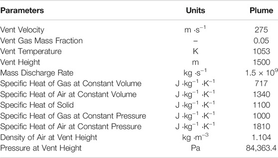
TABLE 1. List of eruption condition and material properties for plume simulation.
Running of Plume-SPH updates physical quantities, such as temperature, velocity, and the position of SPH particles in each time step. During Plume-SPH simulation, SPH particles of phase 2, which represent the erupted material, are injected from the eruption vent into the computation domain with an initial injection velocity. As they move upwards, these particles will get mixed with SPH particles of phase 1, which represent the air, during the whole simulation. Their physics quantities get updated as well. After the simulation, the computation domain will be filled with SPH particles of both phase 1 and phase 2. Removing all SPH particles of phase 1 from the computation domain, all of the remaining SPH particles represent the erupted material, which naturally forms a plume (see Figure 1).
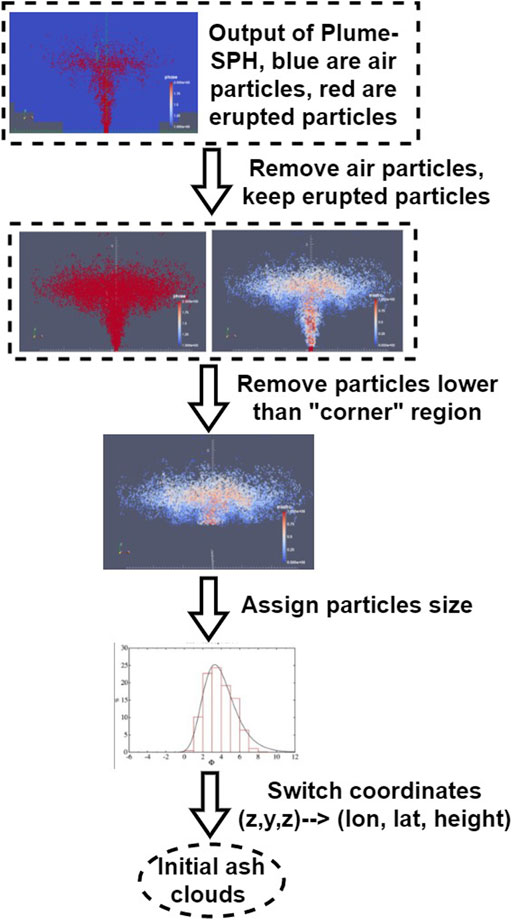
FIGURE 1. Steps to create initial condition for Puff based on raw output of Plume-SPH (Cao et al., 2018). First row: raw output of Plume-SPH. Blue particles are phase 1 (ambient air), and red particles are phase 2 (erupted material). Second row: plume after removing SPH particles of phase 1. Picture at right is colored according to the mass fraction of erupted material. Third row: volcanic plume above the “corner” region after cutting off the lower portion. Fourth row: assign sizes to particles converting numerical discretization points into tracers. Fifth row: switch coordinates in local coordinate system into (longitude, latitude, height).
2.2 Puff and Initial Ash Cloud
Puff (Tanaka, 1991; Searcy et al., 1998) is a dynamic pollutant tracer model. The model is based on a 3D Lagrangian form of the fluid mechanics, in which the material transport is represented by the fluid motion, and diffusion is parameterized by a stochastic process of random walk. Here, the model is constructed by a sufficiently large number of Lagrangian tracer particles with a random variables Ri(t) = (x(t), y(t), z(t)), where i = 1 ∼ M, which represents position vectors of particles from the origin of the ash source at the time t. M is the total number of Lagrangian tracer particles, a sample of all the ash particles.
Here, W accounts for local wind advection, Z is generated by Gaussian random numbers and accounts for turbulent dispersion, and S is the terminal gravitational fallout velocity or settling speed, which depends on a tracer’s size.
A collection of tracer particles can be used to start a Puff simulation. The tracer particles have three basic properties: age, size, and position. The age of each particle is the elapsed time from when it was released. Ash particles in the initial ash cloud have zero age. Initial ash size distribution is assumed to be log-normal. According to a mean and standard deviation provided by the user, Puff assigns size to each particle. Puff initializes the position of each particle according to semiempirical expressions. The height of each particle is determined according to the specified distribution from the surface (1000 mbar ≅ 0 m) to the top of the plume height, Hmax, which is given by the user. Puff also supports reading predefined initial ash clouds from a file, containing the coordinates of all tracer particles.
Vertical particle distribution in Puff is usually based on the Poisson distribution. For the Poisson distribution, the vertical height of ash particles is given by Eq. 13:
where P is an integral value drawn from a Poisson distribution of unit mean, R is a uniformly distributed random number between 0 and 1, Hmax is the maximum plume height, Hwidth represents an approximate vertical range over which the ash will be distributed. So for Poisson distribution, the user can specify two parameters, Hmax and Hwidth. Another commonly used vertical ash distribution in VATD simulation is Suzuki. For the Suzuki plume shape (Suzuki, 1983), the ash mass vertical distribution is assumed to follow the Eq. 14:
where Qm is the total mass of erupted material, k is the shape factor, which is an adjustable constant that controls ash distribution with height. A low value of k gives a roughly uniform distribution of mass with elevation, while high values of k concentrate mass near the plume top. So for Suzuki distribution, besides the plume height Hmax, there is another user-specified parameter, k.
Puff initializes the horizontal distribution of ash particles according to semiempirical expression as well. Puff uses a uniformly distributed random process to determine ash particle locations in a circle centered on the volcano site. The maximum radius (at plume top) at which a particle can be located is given as “horizontal spread”. The horizontal displacement from a vertical line above the volcano is a random value within a circle of which the radius equals the “horizontal spread” multiplied by the ratio of the particle height H to the maximum Hmax, see Eq. 15. So the resulting shape of the particle distribution within the plume is an inverted cone in which particles are located directly over the volcano at the lowest level and extend out further horizontally with increasing plume height.
where r(H) is the radius of the horizontal circle, within which all particles at the height of H are located. rmax is the horizontal spread. H is the height, and R is an uniformly distributed random number between 0 and 1.
In summary, particle distributions in the initial ash cloud are controlled by several parameters, for example, Hmax, Hwidth, and rmax if the user chooses to use semiempirical expressions, Eqs 13, 15. Users can optimize or calibrate these parameters to adjust the initial condition for Puff so that the simulated results match better with observations. Besides the initial ash cloud, other input parameters for Puff are diffusivity in the vertical and horizontal directions, start and end time of the eruption, and eruption duration. When creating initial conditions from the output of Plume-SPH, the total number of Lagrangian tracers is the count of all SPH particles of phase 2 in the plume. The same total number of Lagrangian tracers is used when creating the initial ash cloud based on semiempirical expressions. All input parameters for Puff are listed in Table 2.
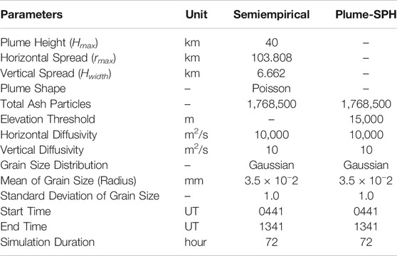
TABLE 2. Parameters used in VATD simulation of the climactic phase of Pinatubo eruption on June 15, 1991. The first six parameters are used by semiempirical expression to create an initial ash cloud. When creating an initial condition based on the Plume-SPH model, these parameters are extracted from output of Plume-SPH model.
2.3 Creation of Initial Ash Cloud From Plume-SPH Output
In this study, we convert the output of Plume-SPH into an initial ash cloud which serves as the initial condition for Puff. The method proposed consists of generating the initial ash cloud directly from Plume-SPH, foregoing assumptions and estimates, or inverse modeling, regarding ash injection height and timing. The steps to create an initial ash cloud based on the raw output of Plume-SPH are shown in Figure 1. The initial ash cloud is created from SPH particles of phase 2, which represents the erupted material in the model. After reaching the maximum rise height and starting to spread horizontally, particles of phase 2 form an initial umbrella cloud (Figure 2). The 3D plume simulation is considered complete once the umbrella cloud begins to form. Parcels that will be transported by the ambient wind are those above the “corner” region, where mean plume motion is horizontal rather than vertical. With such consideration, we introduce an elevation threshold, which is the lower elevation limit of the ash that will be transported by the VATD. All SPH particles with elevation lower than the threshold are excluded when creating the initial ash cloud. The inflection point from vertical raising to horizontal spreading happens around 15 km according to the averaged vertical velocity [(d) in Figure 2] and horizontal velocity [(e) in Figure 2]. Below this inflection point, particle trajectories are primarily vertical in the stalk-like eruption column. Above this level, particle trajectories are primarily horizontal, as they flow into the umbrella cloud gravity current. So we choose 15 km to be the elevation threshold in this study.
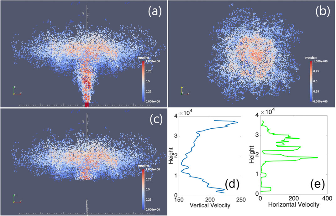
FIGURE 2. Volcano plume from 3D plume model. All particles in the pictures are of phase 2 (particle of phase 1 has been removed) at 600s after eruption, at which time, the plume has already reached the plume height and started spreading radially. (A) is the front view of the whole plume. (B) is the top view of the plume. (C) is the front view of the initial ash cloud, which is essentially a portion of the whole plume whose elevation is higher than a given threshold (in this picture is 15 km). Particles are colored according to mass fraction of erupted material. Red represents high mass fraction while blue represents low mass fraction. (D) is the average vertical velocity of the plume. At elevations below 15 km, the average vertical velocity decreases. At elevations higher than 15 km, the averaged vertical velocity starts increasing. (E) is the average horizontal velocity of the plume. The averaged horizontal velocity becomes obviously larger when elevation is higher than15 km. So the reflection point is somewhere around 15 km.
Considering that SPH particles are only discretization points, each is assigned a grain size according to a given total grain size distribution (TGSD) (Paladio-Melosantos et al., 1996), and a concentration according to the mass and volumetric eruption rate. The Plume-SPH discretization points are thus switched to Puff Lagrangian tracer particles having grain sizes and concentrations. The coordinates of these tracer particles, which are initially in the local Cartesian coordinate system of Plume-SPH, are converted into Puff’s global coordinate system, which is given in terms of (longitude, latitude, height). Puff takes the initial ash cloud, consisting of the collection of Lagrangian tracer particles with grain size and concentration, and propagates from time t to time t + Δt via solution to an advection/diffusion equation (Eq. 12).
To summarize, there are four steps to create an initial ash cloud from the raw output of Plume-SPH:
1) filter by SPH particle type to select SPH particles that represent erupted material (phase 2);
2) filter by a mean velocity threshold to select the upper part (above the “corner” region) dominated by horizontal transport;
3) switch SPH discretization points to Lagrangian tracer particles, by assigning grain size to each particle;
4) convert coordinates of the SPH Lagrangian tracers into the VATDs geographic coordinate system.
The features of the volcanic plume and resulting initial ash cloud used in the case study are shown in Figure 2. It is important to point out that since both Plume-SPH and Puff are based on the Lagrangian method, there is no extra step of conversion between an Eulerian grid and Lagrangian particles.
2.4 Puff Restart
The plume and ash transport models are run at different time scales and length scales. The spatial and temporal resolutions of the plume simulations are much finer than those of the ash transport model. It takes tens of minutes (600 s in this case) for the Pinatubo plume to reach a steady height. However, the eruption persisted for a few hours (9 h for the climactic phase of Pinatubo eruption), and it may be necessary to track ash transport for days following an eruption. At present, it is too computationally expensive to run 3D plume simulations for several hours in real time. In order to handle the difference in time scale, we mimic a continuing eruption with intermittent pulses releasing ash particles. In particular, we restart Puff at an interval of 600 s, i.e., the physical time of the plume simulation to reach a steady height. At every Puff restart, we integrate the output of the last Puff simulation and Plume-SPH into a new ash cloud. This new ash cloud serves as a new initial condition with which to restart a Puff simulation. A sketch demonstrating the overall restart process is shown in Figure 3. The total number of Lagrangian tracer particles used in Puff thus equals the summed number of particles in all releases. The total number of tracer particles is therefore no longer a user-selected parameter. Fero et al. (2008) proposed using more realistic time-dependent plume heights. We do not adopt that strategy here for simplicity, although the idea would be straightforward in execution, given time-dependent eruption conditions.
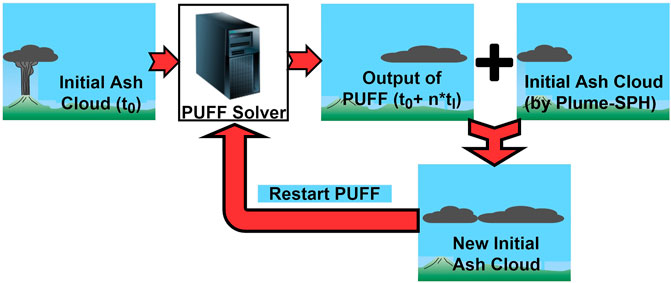
FIGURE 3. Mimic successive eruption with intermittent pulsed releasing of ash particles. tI is the period of pulsing release. tI equals the physical time of 3D plume simulation.
3 Results
The transport of volcanic ash resulting from the Pinatubo eruption on June 15, 1991, is simulated using two different initial conditions. The first type of initial condition is created in a traditional way according to user-specified parameters (Hmax, Hwidth, and rmax) and the semiempirical plume shape expressions (Eqs 13, 15). We use the observed plume height (40 km) as Hmax and take Hwidth = 6.662 km, rmax = 103.808 km, respectively, based on a previous study (Fero et al., 2008). The second type of initial condition is created by the new method proposed in this study. To create initial conditions using the new method described in this study, the plume rise is simulated first by Plume-SPH. Then, the initial ash cloud is obtained by processing the raw output of Plume-SPH following steps described in Creation of Initial Ash Cloud From Plume-SPH Output except for initial conditions, and the parameters that control the VATD simulation are the same for both simulations. Simulated ash transport results are compared against observations.
The simulation results using different initial conditions are compared with TOMS AI (Aerosol Index) and AVHRR BTD (brightness temperature difference) ash cloud map imagery (Figure 4). The Puff simulation results are post-processed by the following steps to calculate the relative concentration.
1) The 3D computational domain is discretized into a collection of cells (latitude, longitude, elevation), and each cell is of size 0.2 degree × 0.2 degree × 1 km;
2) Find the cell that has the maximum number of particles (tracer particles); say the maximum number of particles is Nmax;
3) Exclude all cells that have fewer than five particles, and
4) Calculate the relative concentration of each cell by dividing the number of particles in the cell by Nmax.
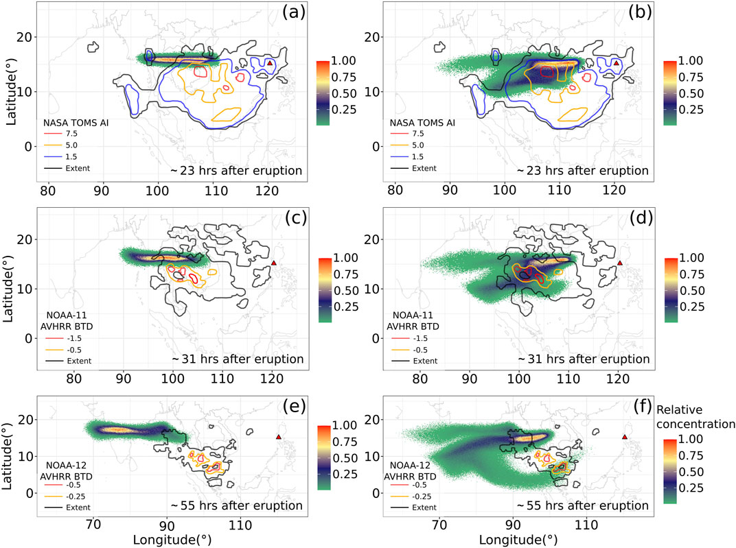
FIGURE 4. Comparison between “Semiempirical initial cloud + Puff” and “Plume-SPH + Puff”. Pictures to the left, (A), (C) and (E), are Puff simulation based on initial condition created according to semiempirical plume shape expression. Pictures to the right, (B), (D) and (F), are Puff simulation based on initial conditions generated by Plume-SPH. TOMS or AVHRR images of Pinatubo ash cloud are overlapped with the simulation results. Ash clouds at different hours after eruption are on different rows. From top to bottom, the images correspond to around 23 h after eruption (UT 199106160341), 31 h after eruption (UT 199106161141), 55 h after eruption (UT 199106171141). The observation data on the first row are TOMS AI (aerosol index) map. The observation data on the second and third row are AVHRR BTD (brightness temperature difference) ash cloud map with atmospheric correction method applied (Guo et al., 2004b). The contours of simulation results are maximum concentration at given (longitude, latitude). The colored dots are simulation results of relative concentrations whose values are between zero to one and have no unit, and the solid contours are observed in Dobson Units.
In contouring, we plot the relative concentration of the cell that has the maximum number of particles at a given (latitude, longitude). In addition to the relative concentration, we also plot the contours of the maximum height of the ash cloud (Figure 5), which is obtained by the following post-processing steps:
1) The 3D computational domain is discretized into a collection of cells (latitude, longitude, elevation), and each cell is of size 0.2 degree × 0.2 degree × 1 km;
2) Exclude all cells that have fewer than five particles, and
3) The maximum height is the cell center height of the top cell among all cells with the same (latitude, longitude).
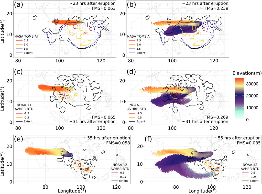
FIGURE 5. Comparison between “Semiempirical initial cloud + Puff” and “Plume-SPH + Puff”. Pictures to the left, (A), (C) and (E), are Puff simulation based on initial condition created according to semiempirical plume shape expression. Pictures to the right, (B), (D) and (F),are Puff simulation based on initial conditions generated by Plume-SPH. TOMS AI (aerosol index) or AVHRR BTD (brightness temperature difference) images of Pinatubo ash cloud are overlapped with the simulation results. Ash clouds at different hours after eruption are on different rows. From top to bottom, the images correspond to around 23 h after eruption (UT 199106160341), 31 h after eruption (UT 199106161141), 55 h after eruption (UT 199106171141). The observation data on the first row are TOMS AI (aerosol index) map. The observation data on the second and third row are AVHRR BTD (brightness temperature difference) ash cloud map with atmospheric correction method applied (Guo et al., 2004b). The colored dots are simulation, and the solid contours are observed in Dobson Units. The contours of simulation results are maximum height of ash cloud, whose unit is m. The FMS value for each simulation is on each contour.
We also calculated the Figure of Merit in Space (FMS) according to the definition:
The differences between simulated ash transport by the “Semiempirical initial cloud + Puff” and “Plume-SPH + Puff” conditions are significant. We first check the maximum relative concentration in Figure 4. At 23 and 31 h after the beginning of the climactic phase, the simulated ash concentration based on the initial conditions created from Plume-SPH is visibly closer to observation than that based on the initial condition generated from semiempirical expressions, especially in terms of the location of the highest concentration region. This is confirmed by the FMS, which is 0.249 (23 h) and 0.269 (31 h) for Plume-SPH results, and 0.063 (23 h) and 0.065 (31 h) for semiempirical initial clouds. Around 55 h after the beginning of the climactic phase, the disparity between observation and simulation becomes more obvious. Ash in the “Semiempirical initial cloud + Puff” simulation is located far west of the observed, with a FMS value equal to 0.058. The high concentration area of the “Plume-SPH + Puff” simulation, even though closer to observation, has also propagated further downwind than in the observation. The FMS goes down to 0.085.
While most of our work is based on the Puff VATD, it is useful to compare the maximum cloud height in Figure 5 with the wind field indicated in the popular VATD, HYSPLIT’s forward trajectory tracking (Figure 6). The comparison reveals that the ash cloud is being transported in two separate, main layers (directions) independently. From Figure 6, we can see that the wind between elevations of 10 and 15 km blew from north-east to south-west, while winds of higher elevation blew from east to west. This vertical wind shear naturally separated the ash cloud into two layers. In the “Semiempirical initial cloud + Puff” results, the lower elevation layer is missing, which is the most important factor causing differences between these two simulation results (Figure 4). Even for the upper layer, the maximum cloud height of the “Semiempirical initial cloud + Puff” simulation results is higher than that of the “Plume-SPH + Puff” simulation. Such differences cannot be captured by metrics based on footprint, such as FMS. At 55 h after the eruption, the observed high concentration ash, which is at a relatively low elevation (inferred from the wind direction at different elevations in Figure 6 and the eruption location), is missing in the “Plume-SPH + Puff” simulation results. This leads to the large decrease of FMS values from 0.269 to 0.085. One possibility is that these ash clouds are from eruptions after the climactic phase. In our current simulation, we use the eruption condition for the climactic phase generating plume height for the climactic phase, but satellites see ash and SO2 from all eruption phases.
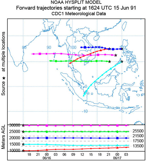
FIGURE 6. Trajectories of particles starting from different heights indicating the wind directions of different evaluations. The trajectories are chosen to start at points that were on the perimeter of the umbrella cloud in x, y, and z, and in its center, right before it became affected by the wind to give an idea of the maximum possible spread of the trajectories from that initial condition.
The only difference in initial conditions between these two simulations is the distribution of ash parcels. The main difference between simulation results from the “Plume-SPH + Puff” and the “Semiempirical initial cloud + Puff” runs can thus be directly attributed to the initial ash particle distribution, which we discuss further in the following section.
3.1 Effect of Plume Height (Hmax)
In this section, we discuss the vertical distribution of ash particles in the initial ash cloud. The majority of volcanic ash particles are usually injected at an elevation lower than the plume height. For instance, Holasek et al. (1996a,b) reported the maximum Pinatubo volcanic plume, i.e., source height, as ∼ 39 km while the distal volcanic cloud heights were estimated at ∼ 20–25 km. Self et al. (1996) reported that the maximum plume height could have been >35 km, but that cloud height was ∼23– 28 km after ∼ 15–16 h. The neutral buoyancy height of the Pinatubo aerosol cloud was estimated with different methods at ∼ 17–26 km (lidar) by DeFoor et al. (1992), ∼ 20–23 km (balloon) by Deshler et al. (1992), ∼ 17–28 km (lidar) by Jäger (1992), and ∼ 17–25 km (lidar) by Avdyushin et al. (1993). Based on a comparison between simulated clouds with early infrared satellite imagery, Fero et al. (2008) reported that the majority of ash was transported between 16 and 18 km. These observations make good physical sense, as particles are concentrated or centered around the intrusion height of the umbrella cloud, not near the plume top, because the plume top is due to momentum overshoot. However, the empirical expressions for the height-MER relation, which are commonly adopted to create initial conditions for VATD simulations, tend to place the majority of ash particles closer to the top if one uses observed plume height in the empirical expressions.
Here, we investigate two commonly used plume shapes, the Poisson (see Eq. 13) and Suzuki (see Eq. 14). Particle distributions (in terms of mass percentage or particle number percentage) in the vertical direction in the initial ash cloud are shown in Figure 7. In that figure, the vertical particle distribution based on Plume-SPH output is compared with the vertical particle distribution based on semiempirical shape expressions. Both Poisson and Suzuki distributions in Figure 7 take Hmax = 40 km, which is close to the reported observed plume height. When adopting the Poisson distribution [(c) in Figure 7], the majority of the particles are between 30 and ∼ 40 km. Obviously, the Poisson function distributes the majority of ash at a higher elevation than was observed (e.g. Fero et al., 2008). As for the Suzuki distribution, (D) in Figure 7, the majority of ash particles also occur in a range that is significantly higher than 25 km. Note that in the plot (d), the Suzuki constant k is set to 4, which is commonly used for Sub-Plinian and Plinian eruption columns (Pfeiffer et al., 2005). As for initial ash clouds in Plume-SPH simulations, most ash particles are distributed between ∼ 17–28 km, which matches well with observations. The plume height is also consistent with observation.
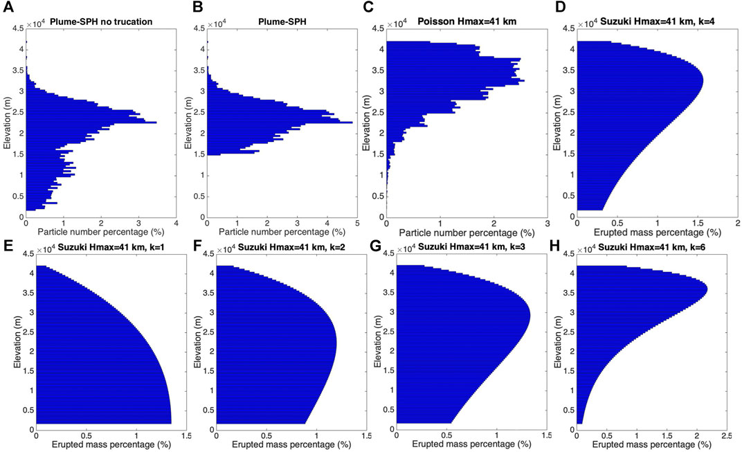
FIGURE 7. First row, comparison of particle distribution of initial ash cloud in vertical direction. (A) is corresponding to the initial ash cloud obtained from Plume-SPH output. (B) is (A) truncated by a elevation threshold of 15 km. (C) is for vertical ash distribution based on Poisson distribution (Eq. 13) with Hmax equals to 40 km. Another parameter, Hwidth is 6662 m. (D) is corresponding to Suzuki distribution (Eq. 14) with Hmax equals to 40 km and k equals to 4 (Pfeiffer et al., 2005). The second row, Suzuki distribution with Hmax equals to 40 km but different values for k. The x axis is the percentage of particle numbers for Plume-SPH and Poisson. For Suzuki, the x axis is the mass percentage of erupted material.
For the Poisson distributions, the ash particles cannot be lower without changing the plume height. To distribute the majority of ash particles at a lower elevation, the plume height must be reduced to a value smaller than the observed plume height. Adjusting parameters such as plume height in the empirical expression is actually the traditional source term of calibration method. A set of initial ash clouds using different plume heights based on the Poisson distribution is shown in Figure 8. The plume heights adopted in plume shape expressions are not obtained from any plume model or observation of plume height, but by a posteriori calibration to later-observed ash cloud transport heights. For Suzuki distribution, adjusting the Suzuki constant can adjust the distribution of ash particles in vertical direction. As shown in Figure 7, when k is equal to 1 [see (e)], the majority of ash particles are at a lower elevation than observation. With k = 3 and k = 6 [figure (g) and (h)], the majority of ash particles are at a higher elevation than observation. When k is set to 2 [see (f)], we can see that the majority of ash particles are roughly distributed in the range 17–28 km. But the shape does not look like a typical plume, as particles are more uniformly distributed in the vertical direction. In addition, the “best fit” Suzuki constant is different from the typical value, which is 4 (Pfeiffer et al., 2005), for Sub-Plinian and Plinian eruptions, meaning that we can not apply previous experiences into the semiempirical expression for this eruption.
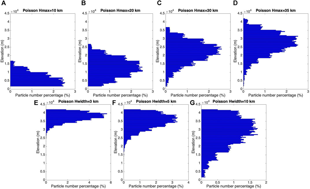
FIGURE 8. Initial particle distribution in vertical direction based on Poisson plume shape (Eq. 13). The first row varies plume heights. (A) to (D) are corresponding to plume height of 10 km, 20 km, 30 km, 35 km. Another parameter, Hwidth is 6662 m for all four figures in the first row. The second row varies “vertical spread”, Hwidth. (E) to (G) are corresponding to vertical spread of 3 km, 5 km, and 10 km. The plume height, Hmax, is set to 40 km for all three figures. The x axis is the percentage of particle numbers. See Figure 7 for vertical ash distribution of Plume-SPH output.
The ash clouds created by the Poisson distribution with different plume heights are used as initial conditions in Puff simulations, whose results are shown in Figure 9. Except for the plume height, all other parameters for creating an initial ash cloud are the same as those in Table 2. Of course, the range over which the majority of ash particles are located is lower when using lower plume heights. Figure 9 thus shows that the plume height has a significant influence on the ash transport simulation. The maximum heights of the simulated ash cloud are completely different when using different Hmax values in the Poisson expression. When the plume height is 10 km, the ash lags behind that observed and its FMS is 0.055, which is very close to FMS when Hmax is 40 km. For the cases that Hmax is 20 and 30 km, the FMS values are 0.121 and 0.142, respectively. Taking 20 km as the plume height better represents the lower elevation portion of the ash cloud while taking 30 km as the plume height better represents the higher elevation portion of the ash cloud.
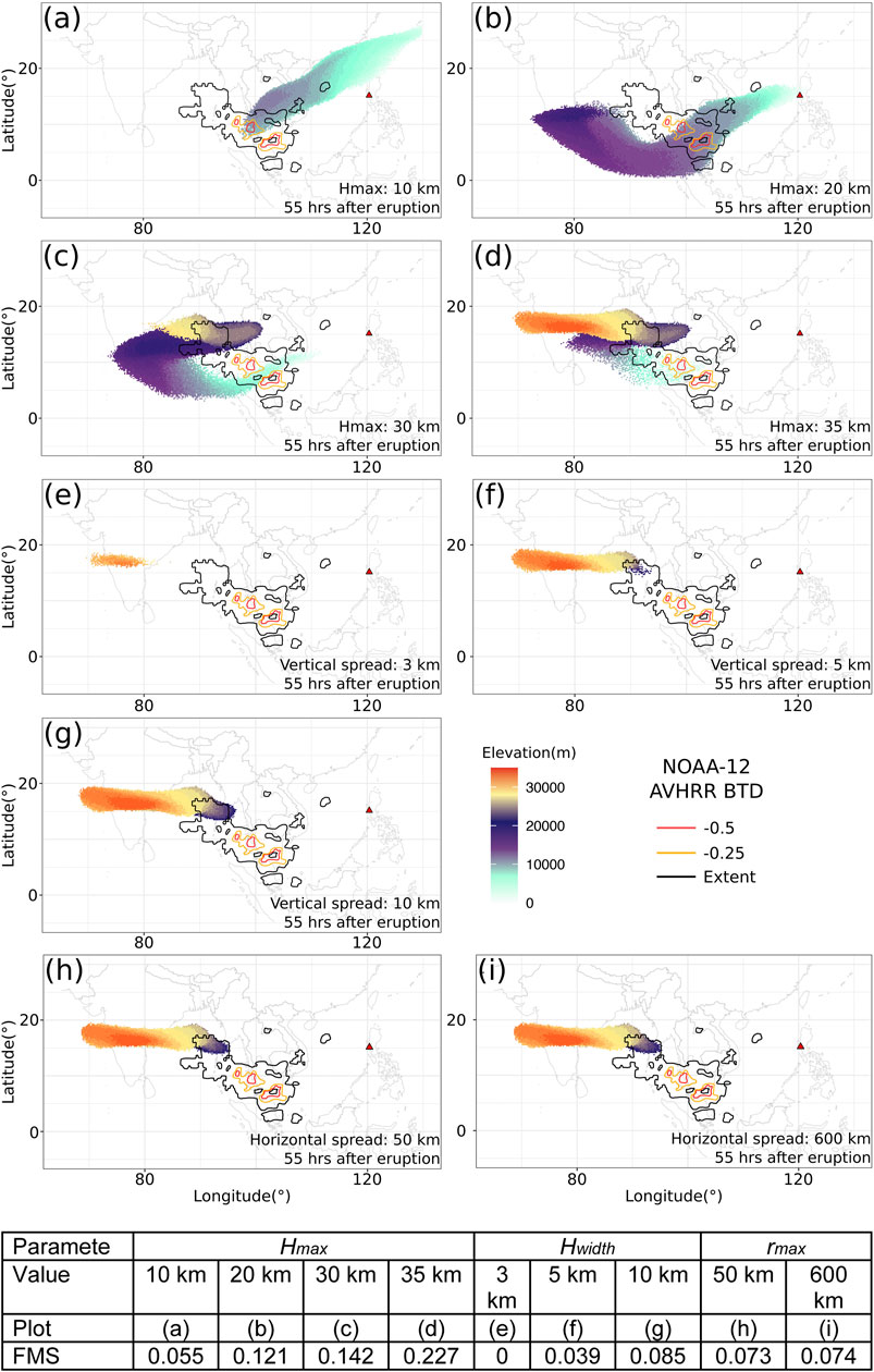
FIGURE 9. Ash transport simulated by Puff using different initial ash clouds created according to the empirical expressions using different input parameters. All images are corresponding to 55 h after eruption (UT 199106171141). More details are in the table.
Simulation results based on a calibrated plume height of 30 km show a footprint similar to those of “Plume-SPH + Puff” although smaller in terms of area. However, the initial ash cloud created by a Poisson distribution with a plume height around 35 km generates the best match with observation in terms of FMS metric, with the FMS value reaching 0.227. That is to say, a plume height lower than the real plume height is required by the Poisson plume shape to distribute ash particles at elevations comparable to the “true” ash distribution. Even for the best-matched results, the high concentration area does not match with an observation well.
It is clear that the initial condition of vertical ash distribution has a dominant effect on VATD simulation, so it is critical for the forecast capability of VATD simulations to explore more accurate and adaptive ways for establishing the initial ash distribution, especially methods that do not rely on a posteriori parameter calibration or inversion.
3.2 Effect of Vertical Spread (Hwidth)
In the previous section, we explored the effects of adjusting the plume height to change the vertical ash distribution at the source. In this section, we investigate the importance of another parameter in the semiempirical Poisson expression (Eq. 13). We vary the “vertical spread”, Hwidth, in the range ∼ 3–10 km. A set of initial ash clouds with different vertical spreads are shown in Figure 8. Except for vertical spread, all other parameters for creating an initial ash cloud are the same as those in Table 2. The vertical range within which the majority of ash particles are located becomes narrower when a smaller value for the vertical spread parameter is used. The ash clouds based on different vertical spread parameters are then used as initial conditions in Puff simulations.
The VATD results are shown in Figure 9. Adjusting the vertical spread changes particle distribution in the vertical direction, and thus, not surprisingly, affects the VATD simulation results. None of the VATD simulations based on initial ash clouds with vertical spreads equal to 3 km or 5 km yield better results than do VATD simulations based on initial conditions created by Plume-SPH (see Figure 9). But when we take 10 km as the vertical spread, we get a FMS that is very close to Plume-SPH, even though the shape of the ash cloud footprint and the maximum height of the ash cloud are completely different.
The calibration tests on vertical spread, carried out here, are certainly not exhaustive. One could do a more comprehensive calibration throughout the multidimensional parameter space (for Poisson distribution, the parameter space is two-dimensional) and find better results. In addition, with a more complicated semiempirical plume shape expression, one could have more control over plume shape and might be able to get an initial condition that yields a more accurate ash transport forecast. However, more complicated and adaptable plume shape expressions imply a higher-dimensional parameter space, which requires more effort in calibration, even though the degrees of freedom to adjust plume shape are still limited. Creating initial conditions based on 3D plume simulations avoids such parameter calibration.
3.3 Horizontal Ash Distribution
The differences between the semiempirical plume particle distribution and actual (or simulated by the 3D plume model) are not only in the vertical direction. The importance of the horizontal distance of each initial ash particle from a line extending upward from the volcano is investigated in this section. Puff uses a uniformly distributed random process to determine ash particle locations in a circle centered on the volcano site as described in Puff and Initial Ash Cloud for the output of Plume-SPH, and an effective (maximum) radius is determined according to a given threshold of ash concentration, following Cerminara et al. (2016b). A time-averaged, spatial integration of the dynamic 3D flow field is conducted to remove significant fluctuations in time and space. Figure 10 compares the radius of the initial ash clouds created by 3D plume simulations with that assumed in the semiempirical plume shape expression adopted in Puff. It is impossible for the simple, assumed plume shapes to capture the complex and more realistic shapes developed by Plume-SPH. Additional parameterization may generate more reasonable shapes, but these would continue to be ad hoc; none would likely have the potential fidelity of the 3D simulation to reality, and adding a temporally changing distribution would be difficult.
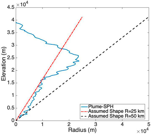
FIGURE 10. Comparison between radius of initial ash clouds created by 3D plume model (Plume-SPH) and assumed initial ash cloud shape (Eq. 15) in Puff. The plume shape expression used in Puff defines an inverted cone whose actual shape changes when “horizontal spread” takes different values. R = 25 km is corresponding to “horizontal spread” equals to 50 km. R = 50 km is corresponding to “horizontal spread” equals to 100 km.
Comparison between cross-sectional views of the initial ash clouds is shown in Figure 11. The cross-sectional view of horizontal particle distribution using the semiempirical method (last figure in Figure 11) is similar to a cross-sectional view of a simulated 3D plume, in a general sense. However, for simulated 3D plumes, the ash particle distribution in cross section varies with height, which factor would become increasingly important with increasing wind speed, where wind speed to be included in the estimate of initial plume shape. It is difficult for the semiempirical expressions to accommodate such a complex distribution.
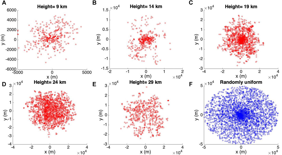
FIGURE 11. Horizontal distribution of ash particles (tracers) on a cross section of initial ash cloud. Puff assumes a randomly uniform distribution of ash particles within a circle, as shown by blue dots in (F). All other figures show the ash particle distribution of initial ash clouds created by Plume-SPH at different elevations.
Despite the obvious difficulty of correctly estimating ash distribution near the vent, or for short propagation times, assigning different values for the horizontal spread has a negligible effect on VATD simulation results at large time. We investigated horizontal spread values between 50 and 1600 km to create initial ash clouds; all of them generated similar results at large propagation times (> 1 day). Figure 9 shows two different simulation results based on initial ash clouds with horizontal spread equal to 50 and 600 km, respectively. No visible differences are apparent between them. The FMS values, 0.073 and 0.074, respectively, are also very close. This implies that horizontal distribution has a less significant influence on VATD simulation results than does vertical distribution for long distance or large time. Perhaps, the most important ramification of this result is that it means the time at which the “handshake” is made between Plume-SPH and the VATD does not affect results significantly for relatively large distances and times.
4 Discussion
4.1 Sentitivity of Other Input Parameters
Besides the initial ash cloud, other parameters for Puff simulations are horizontal diffusivity, vertical diffusivity, mean grain size, grain size standard deviation, and total number of tracers. We present in this subsection informal sensitivity studies on these parameters. We also investigate the influence of eruption duration. The sensitivity analyses will serve as the basis for identifying possible sources of disparities between simulation and observation.
Fero et al. (2008) simulated the volcanic ash transport in the Pinatubo eruption in 1991. He carried out systematic sensitivity analysis with respect to input parameters of Puff and found that all other parameters except for the plume height have negligible effect on long-term ash transportation of Pinatubo. Inspired by Fero et al. (2008), we carried out similar informal sensitivity analysis with much fewer sample points in the parameter space and got similar results. Among the parameters explored, the eruption duration and beginning time show the most obvious influence on simulated ash distribution although the effect is still small. To show the differences in an intuitive way, (a) - (c) in Figure 12 shows simulated ash distribution corresponding to 4.9 h duration, 9 h duration, and 11 h duration, respectively. After 72 h, relative to the simulation starting time, these three cases generate very similar results with tiny visible differences. Daniele et al. (2009) did sensitivity analysis with respect to the input parameters of Puff on different volcanoes and found that for eruptive eruptions, the most dominant factors are the wind field and plume height, while all other input parameters are relatively less important. The significance of the wind field has been confirmed by other researchers (e.g. Stefanescu et al., 2014).
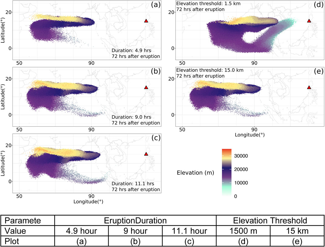
FIGURE 12. Sensitivity of Puff simulation with respect to eruption durations and initial ash cloud cutoff heights (elevation threshold). For different eruption durations, the starting and ending time for each case are in Table 3. The contours correspond to ash concentration at 72 h after eruption. Details are in the table.
We conducted several simulations with eruption duration varying in the range of 5–11 h with slightly different starting time of climactic phase. Table 3 lists all these simulations. However, only slight visible differences are observed among the simulated ash transport outputs. We can see that the eruption duration has negligible effects on long-term ash transport.
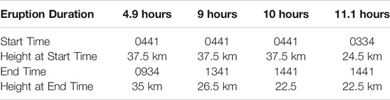
TABLE 3. The starting and ending time (UT) for simulating the climactic phase of Pinatubo eruption on June 15, 1991. Observed plume height (Holasek et al., 1996a) at different times is also listed in the table.
The new methodology for generating initial ash clouds introduces a new parameter: elevation threshold, which was specified based on averaged vertical velocity and horizontal velocity. We carry out a separate, informal sensitivity analysis on this parameter by varying the elevation threshold from 1.5 km (the height of the vent) to 25 km. The simulated ash distributions show obvious differences, especially when the elevation threshold is either very high or very low. However, varying the elevation threshold in the range of 12–18 km generates relatively small differences in ash transport simulation results. Figure 12 (d) and (f) compare the simulated ash distributions corresponding to elevation thresholds of 1.5 and 15 km. Compared with the ash distribution for a threshold of 15 km, an extra-long tail appears when using an elevation threshold of 1.5 km. The maximum height of the tail is around 10 km. Adopting lower elevation thresholds adds more tracer particles at lower elevation. As the winds at different elevations are different, the tracers at lower elevations propagate in different directions. The HYSPLIT forward trajectory tracking indicates that the wind between elevations of 10 and 15 km blew from north-east to south-west, while winds of higher elevation blew from east to west (see Figure 6).
4.2 Other Sources of Disparities
The full range of research issues raised by numerical forecasting of volcanic clouds is diverse. We focused on the effect of initial conditions in this study. During the plume modeling, secondary factors, such as microphysical processes, even though they play lesser roles, likely need to be included to improve accuracy for a particular eruption. Wind fields are not considered in the current version of Plume-SPH, but for weak plumes, wind plays an important enough role that it has to be considered in the plume model. In addition, eruption conditions are subject to change with time, even during the climactic phase of an eruption. For example, ash just west of Pinatubo observed in satellite images does not show up in “Plume-SPH + Puff” simulation results. This disparity is likely due to the fact that Pinatubo continued erupting (with smaller plume height) after the climactic phase, while we only simulate the climactic phase. In the future, time-dependent initial conditions for VATDs can be created from 3D plume simulations based on time-dependent eruption conditions. It is worth mentioning that the eruption conditions at the vent are usually inferred from observable information based on 1D plume models. Using a 3D plume model will not reduce uncertainties from the eruption conditions.
Additional assumptions made during computations in each VATD model or even measurements may also generate additional disparity. Analysis of the results (see large decrease in FMS shown in (f) in Figure 5) indicates that Puff underestimates the fallout of ash particles, which together with satellite pictures not capturing low-level ash clouds can explain the FMS decrease.
One implicit assumption in the current method is that ash transportation is dominated by wind advection (the passive dispersion approximation). However, during the growth of the volcanic umbrella, the dominant factors are various in different regimes (Pouget et al., 2016a) depending on the characteristics of a particular eruption. Webster et al. (2020) suggested that the lateral spread by the intrusive gravity current dominates the transport of the ash cloud in this stage. Studies by Mastin (Mastin et al., 2014; Mastin and Van Eaton, 2020) also showed that neglecting the umbrella cloud formation for larger eruptions led to significantly different footprints for the resulting VATD fallout maps. Their studies imply that including mapped velocities of the plume as a perturbation on the winds can better capture the radial spreading of an umbrella. In the current method, the 3D plume model generated initial ash cloud has a radius of around 25 km. For the Pinatubo 1991 eruption, the passive dispersion approximation can be reasonably applied when radius is greater than 450 km and can be fully valid only when the radius is greater than 1800 km (Costa et al., 2013). So the umbrella stage during the ash transportation is very likely oversimplified in the current simulation. It is computationally too expensive for the Plume-SPH model to continue simulation until the plume radius reaches, at least, for example, 450 km. An additional umbrella model, with a much coarser resolution and simplified physics, in between the plume model and the VATD model would presumably better model the whole ash transportation process.
Besides the errors from assumptions in the model, errors are also introduced from the reanalysis wind field data and the satellite observations, which are retrievals, with their associated errors, rather than the “truth”. In addition, metrics based on footprint cannot account for the disparities at different heights and ash concentrations. Comparing the simulation and observation purely based on footprint-based metric sometimes is biased.
4.3 Summary
Traditional VATD simulations use initial conditions created according to a semiempirical plume shape expression. This study presents, for the first time, VATD simulations using initial source conditions created by a 3D plume model. A case study of the 1991 Pinatubo eruption demonstrates that a 3D plume model can create more realistic initial ash cloud and ash parcel positions and therefore improve the accuracy of ash transport forecasts. Informal sensitivity analyses suggest that initial conditions, as expressed in the disposition of initial ash parcel positions in the vertical, have a more significant effect on a volcanic ash transport forecast than most other parameters. Comparison of initial ash parcel distributions among the 3D plume model, semiempirical expressions, and observations suggests that a major subpopulation of ash parcels should be placed at a much lower elevation than plume height to obtain a better VATD forecast. Comparing the effects of the plume height, vertical spread and horizontal spread show that ash particle distribution in the vertical direction has the strongest effect on VATD simulation results.
To summarize, we have presented a novel method for creating a priori initial source conditions for VATD simulations. We have shown that it might be possible to obtain initial positions of ash parcels with deterministic forward modeling of the volcanic plume, potentially obviating or lessening the need to attempt to somehow observe initial positions, or a posteriori create a history of release heights via inversion (Stohl et al., 2011). Although the method now suffers from the high computational cost associated with 3D forward modeling, there is the possibility that in future it might not only help overcome shortcomings of existing methods used to generate a priori input parameters but also overcome the need to carry out thousands of runs associated with inverse modeling. In addition, computational cost will continue to diminish as computing speed increases. As they are forward numerical models based on first principles, 3D plume models need little if any parameterization, and user intervention should not be required to improve forecast power; no assumption about the initial position of ash parcels is needed. Generation of the initial cloud of ash parcels directly by 3D simulation is potentially adaptable to a variety of volcanic and atmospheric scenarios. In contrast, semiempirical expressions used to determine initial conditions require several parameters to control ash particle distribution along with a vertical line source or some simplified shape of the initial ash cloud, making it difficult in some cases to generate initial conditions that closely resemble a complex reality.
The plume-VATD coupling presented in this study is LagrangianLagrangian coupling. When coupling plume models and VATD models of different types, the interpolation will be different. For example, to couple a Lagarian plume model with an Eulerian VATD model, we must convert the particle distribution in the output of the plume model into ash concentration of cells (mesh grids). When coupling an Eulerian plume model to a Lagrangian VATD model, the mass fraction of the erupted material in the output of the 3D plume model should be converted into an ash cloud represented by a group of particles. The steps for coupling a 3D plume model with a VATD model also depend on features of the software, such as the inputs, the outputs, and file formats.
Data Availability Statement
The raw data supporting the conclusions of this article will be made available by the authors, without undue reservation.
Author Contributions
The idea of using a 3D plume model to start a VATD simulation originated from a conservation between AP and MB. ZC carried out the Plume-SPH simulations, Puff simulations, initial results analysis, and prepared the first draft. All authors worked together for further revisions. MB carried out the HYSPLIT simulation. QY post-processed the Puff simulation results, overlapped the simulation results with satellite observation, and calculated the FMS values. All authors contributed equally to the manuscript writing. AP and MB obtained funding to financially support the work.
Funding
This work was supported by National Science Foundation awards 1521855, 1621853, and 1821311, 1821338, and 2004302 and by the National Research Foundation Singapore and the Singapore Ministry of Education under the Research Centres of Excellence initiative (project number: NRF2018NRF-NSFC003ES-010).
Conflict of Interest
ZC was employed by ANSYS Inc.
The remaining authors declare that the research was conducted in the absence of any commercial or financial relationships that could be construed as a potential conflict of interest.
Publisher’s Note
All claims expressed in this article are solely those of the authors and do not necessarily represent those of their affiliated organizations, or those of the publisher, the editors and the reviewers. Any product that may be evaluated in this article, or claim that may be made by its manufacturer, is not guaranteed or endorsed by the publisher.
Acknowledgments
We are grateful to the two reviewers of the paper for their constructive comments and suggestions that improved the paper. Support for the Twentieth Century Reanalysis Project dataset is provided by the U.S. Department of Energy, Office of Science Innovative and Novel Computational Impact on Theory and Experiment (DOE INCITE) program, and Office of Biological and Environmental Research (BER), and by the National Oceanic and Atmospheric Administration Climate Program Office.
References
Avdyushin, S. I., Tulinov, G. F., Ivanov, M. S., Kuzmenko, B. N., Mezhuev, I. R., Nardi, B., et al. (1993). 1. Spatial and Temporal Evolution of the Optical Thickness of the Pinatubo Aerosol Cloud in the Northern Hemisphere from a Network of Ship-Borne and Stationary Lidars. Geophys. Res. Lett. 20, 1963–1966. doi:10.1029/93gl00485
Bursik, M. (2001). Effect of Wind on the Rise Height of Volcanic Plumes. Geophys. Res. Lett. 28, 3621–3624. doi:10.1029/2001gl013393
Bursik, M. I., Kobs, S. E., Burns, A., Braitseva, O. A., Bazanova, L. I., Melekestsev, I. V., et al. (2009). Volcanic Plumes and Wind: Jetstream Interaction Examples and Implications for Air Traffic. J. Volcanology Geothermal Res. 186, 60–67. doi:10.1016/j.jvolgeores.2009.01.021
Bursik, M., Jones, M., Carn, S., Dean, K., Patra, A., Pavolonis, M., et al. (2012). Estimation and Propagation of Volcanic Source Parameter Uncertainty in an Ash Transport and Dispersal Model: Application to the Eyjafjallajokull Plume of 14-16 April 2010. Bull. Volcanol 74, 2321–2338. doi:10.1007/s00445-012-0665-2
Cao, Z., Patra, A., Bursik, M., Pitman, E. B., and Jones, M. (2018). Plume-sph 1.0: a Three-Dimensional, Dusty-Gas Volcanic Plume Model Based on Smoothed Particle Hydrodynamics. Geosci. Model. Dev. 11, 2691–2715. doi:10.5194/gmd-11-2691-2018
Cao, Z., Patra, A., and Jones, M. (2017). Data Management and Volcano Plume Simulation with Parallel Sph Method and Dynamic Halo Domains. Proced. Comp. Sci. 108, 786–795. doi:10.1016/j.procs.2017.05.094
Cerminara, M., Esposti Ongaro, T., and Neri, A. (2016b). Large Eddy Simulation of Gas–Particle Kinematic Decoupling and Turbulent Entrainment in Volcanic Plumes. J. Volcanology Geothermal Res. 2016, 326. doi:10.1016/j.jvolgeores.2016.06.018
Cerminara, M., Esposti Ongaro, T., and Berselli, L. C. (2016a). Ashee-1.0: a Compressible, Equilibrium-Eulerian Model for Volcanic Ash Plumes. Geosci. Model. Dev. 9, 697–730. doi:10.5194/gmd-9-697-2016
Constantinescu, R., Hopulele-Gligor, A., Connor, C. B., Bonadonna, C., Connor, L. J., Lindsay, J. M., et al. (2021). The Radius of the Umbrella Cloud Helps Characterize Large Explosive Volcanic Eruptions. Commun. Earth Environ. 2, 1–8. doi:10.1038/s43247-020-00078-3
Costa, A., Folch, A., and Macedonio, G. (2013). Density‐driven Transport in the Umbrella Region of Volcanic Clouds: Implications for Tephra Dispersion Models. Geophys. Res. Lett. 40, 4823–4827. doi:10.1002/grl.50942
Costa, A., Suzuki, Y., Cerminara, M., Devenish, B., Esposti Ongaro, T., Herzog, M., et al. (2016). Results of the Eruptive Column Model Inter-comparison Study. J. Volcanology Geothermal Res. 326, 2–25. doi:10.1016/j.jvolgeores.2016.01.017
D’amours, R. (1998). Modeling the Etex Plume Dispersion with the canadian Emergency Response Model. Atmos. Environ. 32, 4335–4341. doi:10.1016/S1352-2310(98)00182-4
Daniele, P., Lirer, L., Petrosino, P., Spinelli, N., and Peterson, R. (2009). Applications of the Puff Model to Forecasts of Volcanic Clouds Dispersal from etna and Vesuvio. Comput. Geosciences 35, 1035–1049. doi:10.1016/j.cageo.2008.06.002
DeFoor, T. E., Robinson, E., and Ryan, S. (1992). Early Lidar Observations of the June 1991 Pinatubo Eruption Plume at Mauna Loa Observatory, hawaii. Geophys. Res. Lett. 19, 187–190. doi:10.1029/91gl02791
de’Michieli Vitturi, M., Neri, A., and Barsotti, S. (2015). Plume-mom 1.0: A New Integral Model of Volcanic Plumes Based on the Method of Moments. Geoscientific Model. Dev. 8, 2447–2463. doi:10.5194/gmd-8-2447-2015
Deshler, T., Hofmann, D. J., Johnson, B. J., and Rozier, W. R. (1992). Balloonborne Measurements of the Pinatubo Aerosol Size Distribution and Volatility at laramie, wyoming during the Summer of 1991. Geophys. Res. Lett. 19, 199–202. doi:10.1029/91gl02787
Draxler, R. R., and Hess, G. (1998). An Overview of The HYSPLIT_4 Modelling System for Trajectories, Dispersion, and Deposition. Aust. Meteorol. Mag. 47, 295–308.
Fero, J., Carey, S. N., and Merrill, J. T. (2009). Simulating the Dispersal of Tephra from the 1991 Pinatubo Eruption: Implications for the Formation of Widespread Ash Layers. J. Volcanology Geothermal Res. 186, 120–131. doi:10.1016/j.jvolgeores.2009.03.011
Fero, J., Carey, S. N., and Merrill, J. T. (2008). Simulation of the 1980 Eruption of Mount St. Helens Using the Ash-Tracking Model Puff. J. Volcanology Geothermal Res. 175, 355–366. doi:10.1016/j.jvolgeores.2008.03.029
Folch, A., Costa, A., and Macedonio, G. (2009). Fall3d: A Computational Model for Transport and Deposition of Volcanic Ash. Comput. Geosciences 35, 1334–1342. doi:10.1016/j.cageo.2008.08.008
Folch, A., Costa, A., and Macedonio, G. (2016). Fplume-1.0: An Integral Volcanic Plume Model Accounting for Ash Aggregation. Geosci. Model. Dev. 9, 431–450. doi:10.5194/gmd-9-431-2016
Gingold, R. A., and Monaghan, J. J. (1977). Smoothed Particle Hydrodynamics: Theory and Application to Non-spherical Stars. Monthly notices R. astronomical Soc. 181, 375–389. doi:10.1093/mnras/181.3.375
Guo, S., Bluth, G. J., Rose, W. I., Watson, I. M., and Prata, A. (2004a). Re-evaluation of So2 Release of the 15 June 1991 Pinatubo Eruption Using Ultraviolet and Infrared Satellite Sensors. Geochem. Geophys. Geosystems 5, 1. doi:10.1029/2003gc000654
Guo, S., Rose, W. I., Bluth, G. J., and Watson, I. M. (2004b). Particles in the Great Pinatubo Volcanic Cloud of June 1991: The Role of Ice. Geochem. Geophys. Geosystems 5, 1. doi:10.1029/2003gc000655
Holasek, R. E., Self, S., and Woods, A. W. (1996a). Satellite Observations and Interpretation of the 1991 Mount Pinatubo Eruption Plumes. J. Geophys. Res. 101, 27635–27655. doi:10.1029/96jb01179
Holasek, R. E., Woods, A. W., and Self, S. (1996b). Experiments on Gas-Ash Separation Processes in Volcanic Umbrella Plumes. J. volcanology geothermal Res. 70, 169–181. doi:10.1016/0377-0273(95)00054-2
Jäger, H. (1992). The Pinatubo Eruption Cloud Observed by Lidar at Garmisch-Partenkirchen. Geophys. Res. Lett. 19, 191–194. doi:10.1029/92gl00071
Jones, A., Thomson, D., Hort, M., and Devenish, B. (2007). “The uk Met Office’s Next-Generation Atmospheric Dispersion Model, Name Iii,” in Air Pollution Modeling and its Application XVII (Springer), 580–589.
Mastin, L. G. (2007). A User-Friendly One-Dimensional Model for Wet Volcanic Plumes. Geochem. Geophys. Geosystems 8, 1. doi:10.1029/2006gc001455
Mastin, L. G., and Van Eaton, A. R. (2020). Comparing Simulations of Umbrella-Cloud Growth and Ash Transport with Observations from Pinatubo, Kelud, and Calbuco Volcanoes. Atmosphere 11, 1038. doi:10.3390/atmos11101038
Mastin, L. G., Van Eaton, A. R., and Lowenstern, J. B. (2014). Modeling Ash Fall Distribution from a Yellowstone Supereruption. Geochem. Geophys. Geosyst. 15, 3459–3475. doi:10.1002/2014gc005469
Neri, A., Esposti Ongaro, T., Macedonio, G., and Gidaspow, D. (2003). Multiparticle Simulation of Collapsing Volcanic Columns and Pyroclastic Flow. J. Geophys. Res. Solid Earth 1978–2012, 108. doi:10.1029/2001jb000508
Oberhuber, J. M., Herzog, M., Graf, H.-F., and Schwanke, K. (1998). Volcanic Plume Simulation on Large Scales. J. Volcanology Geothermal Res. 87, 29–53. doi:10.1016/s0377-0273(98)00099-7
Paladio-Melosantos, M. L. O., Solidum, R. U., Scott, W. E., Quiambao, R. B., Umbal, J. V., Rodolfo, K. S., et al. (1996). Tephra Falls of the 1991 Eruptions of Mount Pinatubo. Fire and mud 12000, 12030.
Pfeiffer, T., Costa, A., and Macedonio, G. (2005). A Model for the Numerical Simulation of Tephra Fall Deposits. J. Volcanology Geothermal Res. 140, 273–294. doi:10.1016/j.jvolgeores.2004.09.001
Pouget, S., Bursik, M., Johnson, C. G., Hogg, A. J., Phillips, J. C., and Sparks, R. S. J. (2016a). Interpretation of Umbrella Cloud Growth and Morphology: Implications for Flow Regimes of Short-Lived and Long-Lived Eruptions. Bull. Volcanol 78, 1–19. doi:10.1007/s00445-015-0993-0
Pouget, S., Bursik, M., Singla, P., and Singh, T. (2016b). Sensitivity Analysis of a One-Dimensional Model of a Volcanic Plume with Particle Fallout and Collapse Behavior. J. Volcanology Geothermal Res. 326, 18. doi:10.1016/j.jvolgeores.2016.02.018
Rolph, G., Stein, A., and Stunder, B. (2017). Real-time Environmental Applications and Display System: Ready. Environ. Model. Softw. 95, 210–228. doi:10.1016/j.envsoft.2017.06.025
Schwaiger, H. F., Denlinger, R. P., and Mastin, L. G. (2012). Ash3d: A Finite-Volume, Conservative Numerical Model for Ash Transport and Tephra Deposition. J. Geophys. Res. Solid Earth 117, 1. doi:10.1029/2011jb008968
Scott, W. E., Hoblitt, R. P., Torres, R. C., Self, S., Martinez, M. M. L., and Nillos, T. (1996). Pyroclastic Flows of the June 15, 1991, Climactic Eruption of Mount Pinatubo. Philippines: Fire and Mud: eruptions and lahars of Mount Pinatubo, 545–570.
Searcy, C., Dean, K., and Stringer, W. (1998). PUFF: A High-Resolution Volcanic Ash Tracking Model. J. Volcanology Geothermal Res. 80, 1–16. doi:10.1016/s0377-0273(97)00037-1
Self, S., Zhao, J.-X., Holasek, R. E., Torres, R. C., and King, A. J. (1996). The Atmospheric Impact of the 1991 Mount Pinatubo Eruption.
Stefanescu, E. R., Patra, A. K., Bursik, M., Jones, M., Madankan, R., Pitman, E. B., et al. (2014). Fast Construction of Surrogates for UQ Central to DDDAS- Application to Volcanic Ash Transport1. Proced. Comp. Sci. 29, 1227–1235. doi:10.1016/j.procs.2014.05.110
Stein, A. F., Draxler, R. R., Rolph, G. D., Stunder, B. J. B., Cohen, M. D., and Ngan, F. (2015). NOAA's HYSPLIT Atmospheric Transport and Dispersion Modeling System. Bull. Am. Meteorol. Soc. 96, 2059–2077. doi:10.1175/bams-d-14-00110.1
Stohl, A., Prata, A. J., Eckhardt, S., Clarisse, L., Durant, A., Henne, S., et al. (2011). Determination of Time- and Height-Resolved Volcanic Ash Emissions and Their Use for Quantitative Ash Dispersion Modeling: the 2010 Eyjafjallajökull Eruption. Atmos. Chem. Phys. 11, 4333–4351. doi:10.5194/acp-11-4333-2011
Suzuki, T. (1983). A Theoretical Model for Dispersion of Tephra. Arc volcanism: Phys. tectonics 95, 113.
Suzuki, Y. J., Koyaguchi, T., Ogawa, M., and Hachisu, I. (2005). A Numerical Study of Turbulent Mixing in Eruption Clouds Using a Three-Dimensional Fluid Dynamics Model. J. Geophys. Res. Solid Earth 110, 1. doi:10.1029/2004jb003460
Suzuki, Y., and Koyaguchi, T. (2009). A Three-Dimensional Numerical Simulation of Spreading Umbrella Clouds. J. Geophys. Res. Solid Earth 1978–2012, 114. doi:10.1029/2007jb005369
Tanaka, H. (1991). “Development of a Prediction Scheme for the Volcanic Ash Fall from Redoubt Volcano,” in First Int’l. Symp. On Volcanic Ash and Aviation Safety, 58.
Tupper, A., Itikarai, I., Richards, M., Prata, F., Carn, S., and Rosenfeld, D. (2007). Facing the Challenges of the International Airways Volcano Watch: the 2004/05 Eruptions of Manam, papua new guinea. Weather Forecast. 22, 175–191. doi:10.1175/waf974.1
Walko, R., Tremback, C., and Bell, M. (1995). Hypact: The Hybrid Particle and Concentration Transport Model. User’s guide. Available at: https://scholar.google.com/scholar?hl=en&as_sdt=0%2C30&q=Hypact%3A+The+Hybrid+Particle+and+Concentration+Transport+Model.+User%E2%80%99s+guide.&btnG=
Webster, H. N., Devenish, B. J., Mastin, L. G., Thomson, D. J., and Van Eaton, A. R. (2020). Operational Modelling of Umbrella Cloud Growth in a Lagrangian Volcanic Ash Transport and Dispersion Model. Atmosphere 11, 200. doi:10.3390/atmos11020200
Witham, C. S., Hort, M. C., Potts, R., Servranckx, R., Husson, P., and Bonnardot, F. (2007). Comparison of VAAC Atmospheric Dispersion Models Using the 1 November 2004 Grimsvötn Eruption. Met. Apps 14, 27–38. doi:10.1002/met.3
Woods, A. W. (1988). The Fluid Dynamics and Thermodynamics of Eruption Columns. Bull. Volcanol 50, 169–193. doi:10.1007/bf01079681
Keywords: volcano, 3D plume model, initial conditions, numerical simulation, SPH, Pinatubo, ash transport, ash dispersal
Citation: Cao Z, Bursik M, Yang Q and Patra A (2021) Simulating the Transport and Dispersal of Volcanic Ash Clouds With Initial Conditions Created by a 3D Plume Model. Front. Earth Sci. 9:704797. doi: 10.3389/feart.2021.704797
Received: 03 May 2021; Accepted: 25 August 2021;
Published: 23 September 2021.
Edited by:
Sara Barsotti, Icelandic Meteorological Office, IcelandReviewed by:
Frances Beckett, Met Office, United KingdomHans Schwaiger, United States Geological Survey (USGS), United States
Copyright © 2021 Cao, Bursik, Yang and Patra. This is an open-access article distributed under the terms of the Creative Commons Attribution License (CC BY). The use, distribution or reproduction in other forums is permitted, provided the original author(s) and the copyright owner(s) are credited and that the original publication in this journal is cited, in accordance with accepted academic practice. No use, distribution or reproduction is permitted which does not comply with these terms.
*Correspondence: Abani Patra, YWJhbmkucGF0cmFAdHVmdHMuZWR1