 Xu Hong-Qiao
 Wang Xiao-Yi1,2,3
- 1Key Laboratory of Petroleum Resources Research, Institute of Geology and Geophysics, Chinese Academy of Sciences, Beijing, China
- 2Innovation Academy for Earth Science, Chinese Academy of Sciences, Beijing, China
- 3University of Chinese Academy of Sciences, Beijing, China
Least-squares reverse time migration (LSRTM) is powerful for imaging complex geological structures. Most researches are based on Born modeling operator with the assumption of small perturbation. However, studies have shown that LSRTM based on Kirchhoff approximation performs better; in particular, it generates a more explicit reflected subsurface and fits large offset data well. Moreover, minimizing the difference between predicted and observed data in a least-squares sense leads to an average solution with relatively low quality. This study applies L1-norm regularization to LSRTM (L1-LSRTM) based on Kirchhoff approximation to compensate for the shortcomings of conventional LSRTM, which obtains a better reflectivity image and gets the residual and resolution in balance. Several numerical examples demonstrate that our method can effectively mitigate the deficiencies of conventional LSRTM and provide a higher resolution image profile.
Introduction
Seismic migration is an inverse procedure of forward modeling, which can restore the interior of the earth medium with record data. Specifically, migration attempts to eliminate the effects caused by the process of physical propagation and obtain an image that clearly depicts the structural information of interest. Reverse time migration (RTM), a state-of-the-art seismic imaging method (Baysal et al., 1983; McMechan, 1983), identifies the aforementioned acausal procedure appropriately. Based on two-way wave equation, RTM is powerful for handling complex geological settings and velocity with dramatic variation in the lateral direction. Therefore, it can deal with steep dips and salt dome better than conventional migration (Zhu and Lines, 1998; Yoon et al., 2003; Liu et al., 2010). However, most migration methods, including RTM, use the adjoint operator to compute the image instead of the inverse operator (Tarantola, 1984). Practical data suffers from many factors, such as irregular acquisition geometry and limited aperture of the acquisition system. These deficiencies generate artifacts and degrade the resolution. To overcome these limitations, least-squares migration (LSM) was proposed to combine with RTM (Liu et al., 2011; Dai et al., 2012). Therefore, seismic imaging can be regarded as a linearized inverse problem. With a proper initial velocity model, seismic records can be inverted to a more accurate profile. LSRTM iteratively reduces the residual between predicted data and observed data in a least-squares framework; therefore, the adjoint operator can keep approaching the inverse operator. Many results have indicated that LSRTM has a better performance than conventional RTM and migration (Zhang et al., 2015; Dutta and Schuster, 2014; Liu et al., 2016).
The precondition of seismic inversion is forward modeling, which maps the parameter model to seismic data. There are two main approaches to build linear approximation between physical model and wavefield (Yang and Zhang, 2019). One is the most commonly used Born approximation based on small perturbation (Beylkin, 1985; Bleistein, 1987). This requires that high-order scattered wavefields are much weaker than primary field. The Born operator describes a linear relationship between model perturbation and primary reflected wave. It divides the wavefield into two parts: background wavefield and perturbation wavefield. LSRTM based on Born approximation can achieve model perturbation with these two fields. In addition, an alternative scheme for modeling is Kirchhoff approximation (Bleistein, 1987). Compared with Born modeling, the Kirchhoff operator delineates the connection between primary reflected wave and reflectivity. Different operators lead to distinctive results under these two physical contexts. However, neither Born nor Kirchhoff approximation can avoid the impact on seismic image in a least-squares sense. Because minimizing the L2 norm only provides an average solution (Wang, 2016; Wu et al., 2016). It is essential to seek a balance between the residual and resolution. According to geological recognition, the earth medium usually presents a layered spatial distribution. The reflection coefficient that mirrors strata attributes should be sparsity, that is, the part of model that does not generate reflected wave ought to be zero. Therefore, the inverted model needs a sparse limitation.
This study implements a Kirchhoff modeling formula for LSRTM promoted by sparsity. The reflectivity model should be regularized with L1 norm while minimizing the residual of wavefield in the form of the L2 norm. Referring to ‘least absolute shrinkage and selection operator’ (Lasso) problem (Tibshirani, 1996), this reformed LSRTM can be solved by the algorithm of spectral projected gradient for L1 minimization (SPGL1), which is designed to solve sparse least squares (van den Berg and Friedlander, 2011). Examples show that our method can effectively overcome the problems mentioned above.
Method
RTM has great advantages in imaging steep strctures such as salt dome. However, it suffers from low-frequency noise compared to conventional migration. Least-squares migration can get closer iteratively to the optimal solution and eventually obtain a relatively high signal-to-noise ratio, high resolution and amplitude equalized profile that eliminates the influence of the acquisition system. It contains three steps: constructing a linear modeling problem first, using the forward and backward propagation wavefields to image, and finally updating the physics model according to the residual.
Linear Modeling Operators
The linearization of nonlinear forward problem is essential to seismic inversion, making the physical progress more explicit; moreover, converting the medium parameter becomes easier. The choice of a linear operator will lead to different physical significance and images. It is a common way to use Born approximation to realize linearization. The real velocity model is divided into two parts: background velocity
where
where
where the
Born approximation represents scattered phenomenon caused by model perturbation, which could be a means of linearizing seismic inversion. However, this approximation is accurate when scattered field
Compared to the Born operator, the Kirchhoff operator relates the reflectivity to wavefield perturbation. Therefore, it depicts the interaction between the incident field and reflectivity rather than velocity perturbation. There is a relationship between reflectivity and model perturbation when the perturbation and incident angle are small (Stolt and Weglein, 2012):
where the
Here we turn Kirchhoff modeling equation into the same form as Born approximation. Then Eq. 7 can be rewritten as.
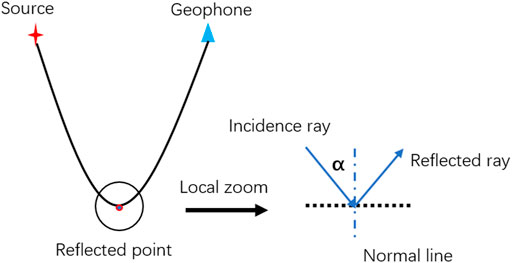
FIGURE 1. Schematic illustration of incident wave and reflected wave. And
It should be noted that the term
Each shot can invert a reflectivity image, here we sum the images obtained by all shots. Then, we regard the summation as the final reflectivity model and use it to iterate. Approximately, we can get an averaged reflectivity model by multiple shots stacking. Therefore, we can get the predicted data by using this stacked reflectivity
With this approximate reflectivity
In sum, with the relationship of reflectivity and model perturbation, two linear approximations have a similar form, which expresses their common ground. The difference between two approximations is also evident. From Eq. 6,
Least-Squares With Sparse Optimization
In contrast to full waveform inversion (FWI) (Liu, et al., 2020), LSRTM first establishes a linear relationship between physical model and corresponding response (Tarantola, 1984), then it implements the inverse problem. The least-squares method (LSM) only requires the construction of a migration operator and inverse migration operator, which is conjugated to each other. It can reduce the residual between the observed and predicted data iteratively to approach the optimal solution of the inverse problem gradually. According to the linear approximation above, we can express them in the form of a matrix:
where the
The model
Where
According to Eq. 13, we can obtain a least-squares solution
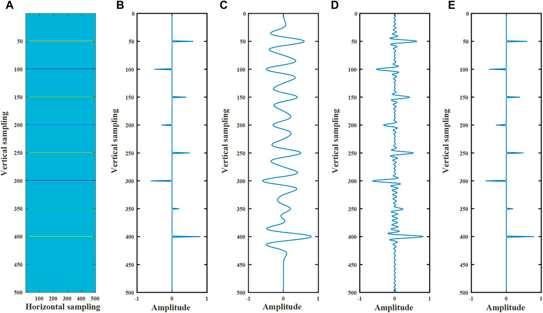
FIGURE 2. (A) reflectivity model; (B) reflection coefficient series extracted in Figure 2A; (C) deconvolution of single record; (D) the result inverted by LSM; (E) the result inverted by sparse constrained LSM.
Due to the feasibility and sparse property of L1-norm, we modify the objective function with L1 norm to realize sparse reconstruction of the model in this study. Generally, Eq. 13 can be reformed with two new problems.
1 Basis Pursuit (BP) problem
where the
2 Least Absolute Shrinkage and Selection Operator (LASSO) problem
where the
Both problems mentioned above can be solved by the algorithm of spectral projected gradient for L1 minimization (SPGL1). Given a constraint
Let
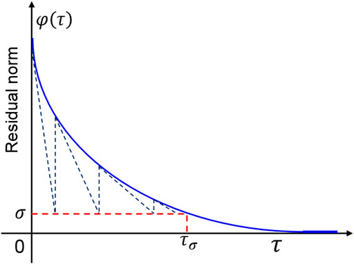
FIGURE 3. Schematic diagram of the Pareto curve. A Newton-based root-finding method is used to update the solution of Eq. 20.
For a given
Here we summarize the workflow of L1-regularized LSRTM as follows:
1) Obtain the predicted data
2) Set the initial model
3) Input the parameters of
4) Solve the Lasso problem
5) Output the result
Numerical Example
In this study, two theoretical models are used to test the validity of the proposed method, including a single diffraction point and complex fault model. Both are based on the two-way acoustic wave equation. Here we use the finite difference method on regular grid.
Single-Diffraction Point
To verify the effectiveness of this method, we first set a simple model with a diffraction point of 2000 m/s embedded in the background velocity of 1,000 m/s (Figure 4), and the entire model has been discretized into 201 × 201 grids in the horizontal and vertical directions, respectively, with the same interval of 5m. The geometry system is arranged as follows: a total of 21 shots are uniformly distributed on the surface of this model with an interval of 50m. Geophones are also placed on each grid point on the surface. We use the Ricker wavelet with a center frequency of 25 Hz for modeling, and the sampling interval is 0.5 ms. In this example, we set 1,000 m/s as the migration velocity.
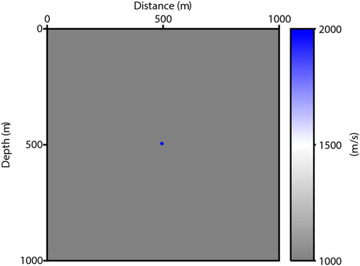
FIGURE 4. A simple diffraction point velocity model.
As shown in Figure 5A, the image is obtained by LSRTM based on Born approximation. This is consistent with the actual situation to a certain degree. The single scatter point is blurred with a disturbing cross pattern (marked by a yellow arrow). However, it should be a dot on the image (Lecomte and Kjeller, 2008). This is because we use the adjoint operator to migrate rather than the inverse operator in Eq. 14. Specifically, Eq. 13 defines a normal equation with
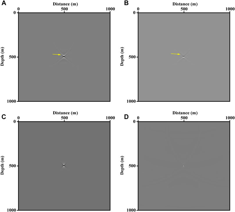
FIGURE 5. The images invert by LSRTM and LSRTM with L1 norm constraint based on Born and Kirchhoff approximation. (A) Unconstrained LSRTM based on Born approximation. (B) Unconstrained LSRTM using Kirchhoff approximation. (C) The image of the LSRTM with L1 norm regularization based on Born approximation. (D) The migrated image with sparse constrained LSRTM based on Kirchhoff approximation.
The LSRTM based on the Kirchhoff operator inverts the reflectivity directly from the seismic records. Figure 5B displays the image produced by Kirchhoff approximation. Compared to Figure 5A, least-squares RTM based on Kirchhoff operator suffers from the same problems. Similarly, we implement the L1 norm on LSRTM, which is shown in Figure 5D. The cross pattern is eliminated clearly, and we obtain an explicit dot rather than a blurred spot. Therefore, for a simple model, the sparsity-promoting LSRTM based on Kirchhoff approximation can effectively improve the resolution of the image. The results calculated by LSRTM in Figures 5A,B iterate 5 times. Figures 5C,D use the SPGL1 algorithm for iterating 10 times with
Fault Model
We also test the other relative complex model. In this fault model (Figure 6A), there are some classical geological structures, including folds, fault blocks, and depressions. Therefore, it appropriately shows the complex structure of near-surface media. The maximum and minimum velocities are 4,000 m/s and 1,500 m/s, respectively. Similarly, we discretize it into 265 × 367 grids with an interval of 5 m. Thus, a total of 25 shots are uniformly located at the surface of this model. The modeling seismic wavelet is same to last experiment.
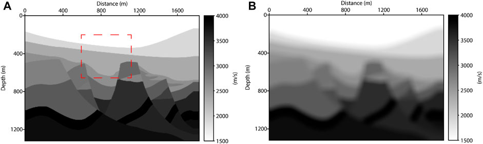
FIGURE 6. (A) The real velocity of fault model. (B) the background velocity model after smooth.
As shown in Figures 7A,B, images inverted by LSRTM based on two approximations fit the fault model well, and the contact relationship between structures can be clearly depicted. To further improve the resolution of these images, we combined L1 norm regularization with LSRTM to reconstruct the model. From Figures 7C,D, the method based on Kirchhoff approximation recovers the stratum’s sparsity more effectively. The results in Figures 7A,B are calculated by LSRTM with 10 iterations. Figures 7C,D use the SPGL1 algorithm for iterating 10 times with
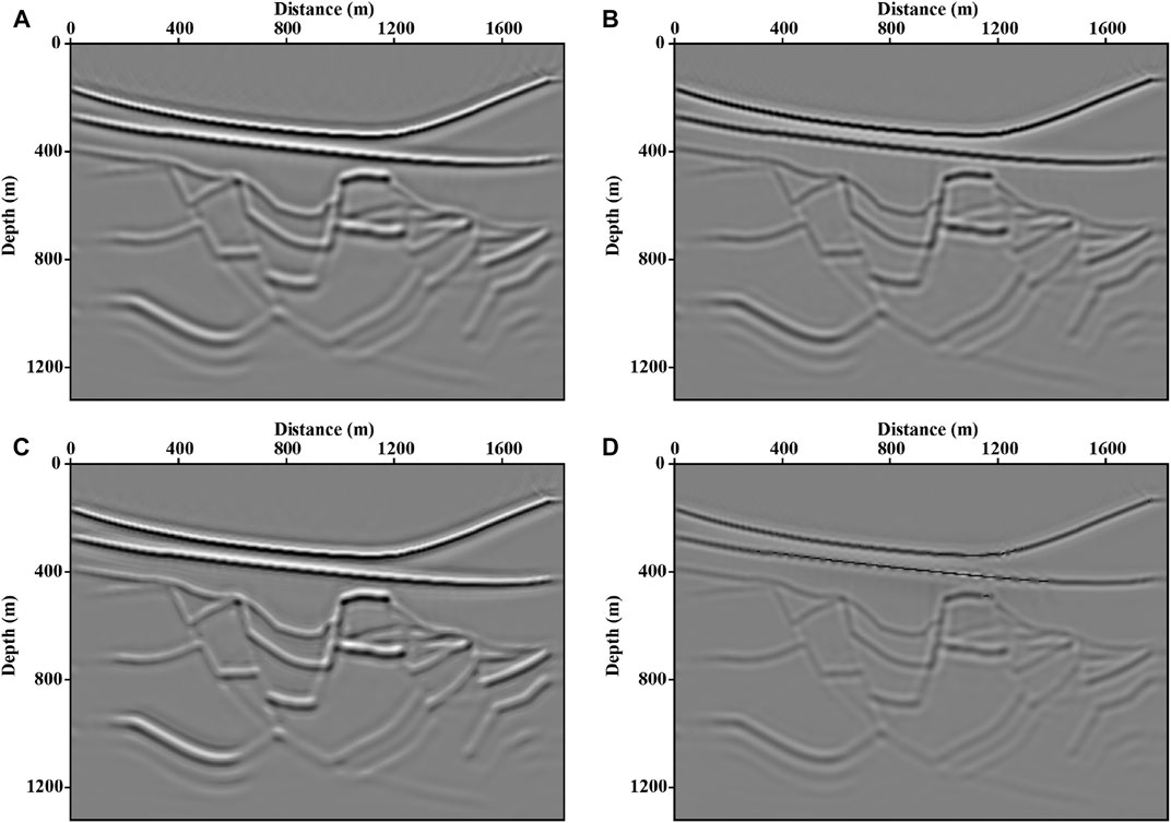
FIGURE 7. Fault images inverted by (A) Unconstrained LSRTM based on Born approximation. (B) Unconstrained LSRTM with Kirchhoff approximation. (C) LSRTM with L1 norm regularization based on Born approximation. (D) sparse constrained LSRTM based on Kirchhoff approximation.
Furthermore, we enlarge the model framed by red rectangle in Figure 6A, which has step-like strata (marked by yellow arrows in Figure 8A). After inverting, the reflectivity image in Figure 8D produced by constrained LSRTM based on Kirchhoff operator agrees with the actual situation.
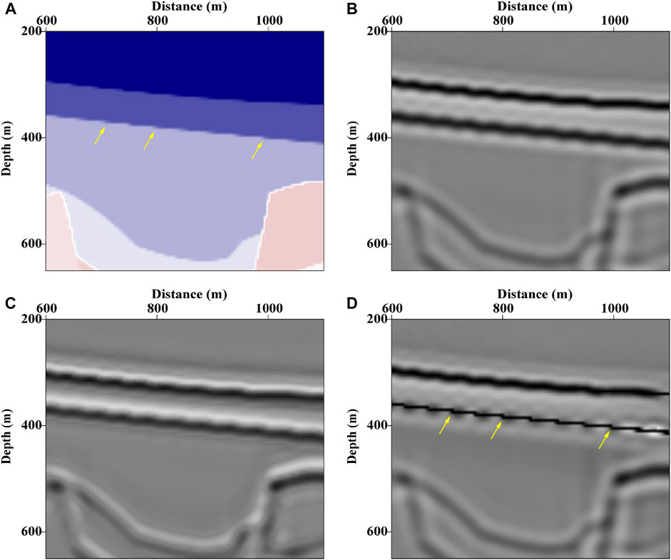
FIGURE 8. (A) true velocity model in the red rectangle in Figure 6A, (B) corresponding image inverted by LSRTM based on Kirchhoff approximation, (C) LSRTM with sparse constraint based on Born approximation, (D) LSRTM with sparse constraint based on Kirchhoff approximation.
Furthermore, images inverted by two different approximations have different phases. According to Eq. 6, reflectivity can be derived from model perturbation. With the assumption of a small incident angle,
Figure 9 shows the amplitude spectra of the images in Figures 7B–D, respectively. The spectra curves are the sum of each trace by the spatial Fourier transform along the depth. The red one is generated from the image inverted by L1-regularized LSRTM based on Born approximation. The blue and green spectrum curves are produced by unconstrained and constrained LSRTM with Kirchhoff approximation, respectively. Because of the spatial derivative and sparse constraint, the spectrum of the image inverted by L1-LSRTM with Kirchhoff approximation has more high-wavenumber components than that of Born approximation, which explains that Kirchhoff approximation improves the resolution of the image.
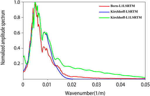
FIGURE 9. The spectrum of inverted images form Figure 6.
Conclusion
The LSRTM recasts classical seismic inversion as a linear inverse problem. By means of linear approximation, physical model is related to the corresponding wavefield. Thereafter, we can reduce the residual between predicted and observed data iteratively to directly invert the interest parameters. This study introduces two linearization methods. Born approximation obtains the relationship between the model and physical response based on perturbation theory. With the help of the Born operator, we derive another type of linear method, namely the Kirchhoff operator, which relates the reflectivity to wavefield explicitly. Moreover, these two methods have a relationship of a spatial derivative, and there is a phase shift between perturbation model and reflectivity model. Although two operators are different physical quantities, the resolution can be improved by Kirchhoff approximation.
LSRTM can mitigate the shortcomings of other migration methods, while the solution is smooth and deviates from the true model. Specifically, there are redundant oscillatory axes in the strata that should be sparsely distributed. Therefore, we reform the question as a sparsity-promoting LSRTM. The SPGL1 algorithm can effectively solve this problem and invert a sparse image that matches the model well. Examples prove the validity of our study.
Data Availability Statement
The raw data supporting the conclusions of this article will be made available by the authors, without undue reservation.
Author Contributions
XH-Q: Methodology, Investigation, Formal analysis, Visualization, Writing—Original Draft WX-Y: Conceptualization, Writing—Review and Editing, Project administration WC-Y: Validation, Data Curation, Writing—Review and Editing ZJ-J: Supervision, Writing—Review and Editing, Funding acquisition.
Conflict of Interest
The authors declare that the research was conducted in the absence of any commercial or financial relationships that could be construed as a potential conflict of interest.
Publisher’s Note
All claims expressed in this article are solely those of the authors and do not necessarily represent those of their affiliated organizations, or those of the publisher, the editors and the reviewers. Any product that may be evaluated in this article, or claim that may be made by its manufacturer, is not guaranteed or endorsed by the publisher.
Acknowledgments
We thank the National Natural Science Fund of China (under grant 42074158) for supporting this work. And we are grateful for the comments provided by reviewers, which improve the quality of this paper a lot.
References
Baysal, E., Kosloff, D. D., and Sherwood, J. W. C. (1983). Reverse Time Migration. Geophysics 48, 1514–1524. doi:10.1190/1.1441434
Beylkin, G. (1985). Imaging of Discontinuities in the Inverse Scattering Problem by Inversion of a Causal Generalized Radon Transform. J. Math. Phys. 26, 99–108. doi:10.1063/1.526755
Bleistein, N., Cohen, J. K., and Hagin, F. G. (1987). Two and One‐half Dimensional Born Inversion with an Arbitrary Reference. Geophysics 52, 26–36. doi:10.1190/1.1442238
Bleistein, N. (1987). On the Imaging of Reflectors in the Earth. Geophysics 52, 931–942. doi:10.1190/1.1442363
Dai, W., Fowler, P., and Schuster, G. T. (2012). Multi-source Least-Squares Reverse Time Migration. Geophys. Prospecting 60, 681–695. doi:10.1111/j.1365-2478.2012.01092.x
Dutta, G., and Schuster, G. T. (2014). Attenuation Compensation for Least-Squares Reverse Time Migration Using the Viscoacoustic-Wave Equation. Geophysics 79, S251–S262. doi:10.1190/geo2013-0414.1
Jiang, B., and Zhang, J. (2019). Least-squares Migration with a Blockwise Hessian Matrix: A Prestack Time-Migration Approach. Geophysics 84, R625–R640. doi:10.1190/geo2018-0533.1
Lecomte, I. (2008). Resolution and Illumination Analyses in PSDM: A ray-based Approach. The Leading Edge 27, 650–663. doi:10.1190/1.2919584
Liu, H. W., Li, B., Liu, H., Tong, X. ‐L., and Liu, Q. (2010). The Algorithm of High Order Finite Difference Pre-stack Reverse Time Migration and GPU Implementation. Chin. J. Geophys. 53, 1725–1733. doi:10.1002/cjg2.1530(in Chinese)
Liu, Y., Chang, X., Jin, D., He, R., Sun, H., and Zheng, Y. (2011). Reverse Time Migration of Multiples for Subsalt Imaging. Geophysics 76, WB209–WB216. doi:10.1190/geo2010-0312.1
Liu, Y., He, B., and Zheng, Y. (2020). Controlled-order Multiple Waveform Inversion. Geophysics 85, R243–R250. doi:10.1190/geo2019-0658.1
Liu, Y., Liu, X., Osen, A., Shao, Y., Hu, H., and Zheng, Y. (2016). Least-squares Reverse Time Migration Using Controlled-Order Multiple Reflections. Geophysics 81, S347–S357. doi:10.1190/geo2015-0479.1
McMechan, G. A. (1983). Migration by Extrapolation of Time-dependent Boundary Values*. Geophys. Prospect 31, 413–420. doi:10.1111/j.1365-2478.1983.tb01060.x
Plessix, R.-E. (2006). A Review of the Adjoint-State Method for Computing the Gradient of a Functional with Geophysical Applications. Geophys. J. Int. 167, 495–503. doi:10.1111/j.1365-246X.2006.02978.x
Schuster, G. T. (2017). Seismic Inversion. Tulsa: Society of Exploration Geophysicists. doi:10.1190/1.9781560803423
Stolt, R. H., and Weglein, A. B. (2012). Seismic Imaging and Inversion: Application of Linear Inverse Theory. New York: Cambridge University Press, 1–404. doi:10.1017/CBO9781139056250
Tarantola, A. (1984). Inversion of Seismic Reflection Data in the Acoustic Approximation. Geophysics 49, 1259–1266. doi:10.1190/1.1441754
Tibshirani, R. (1996). Regression Shrinkage and Selection via the Lasso. J. R. Stat. Soc. Ser. B (Methodological) 58, 267–288. doi:10.1111/j.2517-6161.1996.tb02080.x
van den Berg, E., and Friedlander, M. P. (2009). Probing the Pareto Frontier for Basis Pursuit Solutions. SIAM J. Sci. Comput. 31, 890–912. doi:10.1137/080714488
van den Berg, E., and Friedlander, M. P. (2011). Sparse Optimization with Least-Squares Constraints. SIAM J. Optim. 21, 1201–1229. doi:10.1137/100785028
Wang, X. Y., Zhang, J. J., Xu, H. Q., and Tian, B. Q. (2021). Least-squares Reverse Time Migration with Wavefield Decomposition Based on the Poynting Vector. Chin. J. Geophys. (in Chinese) 64, 645–655. doi:10.6038/cjg2021O0120
Wang, Y. H. (2016). Seismic Inversion: Theory and Applications. Oxford: Wiley, 85–86. doi:10.1002/9781119258032.ch7
Wu, D., Yao, G., Cao, J., and Wang, Y. (2016). Least-squares RTM with L1 Norm Regularisation. J. Geophys. Eng. 13, 666–673. doi:10.1088/1742-2132/13/5/666
Yang, K., and Zhang, J. (2019). Comparison between Born and Kirchhoff Operators for Least-Squares Reverse Time Migration and the Constraint of the Propagation of the Background Wavefield. Geophysics 84, R725–R739. doi:10.1190/geo2018-0438.1
Yoon, K., Shin, C., Suh, S., Lines, L. R., and Hong, S. (2003). 3D Reverse-Time Migration Using the Acoustic Wave Equation: An Experience with the SEG/EAGE Data Set. The Leading Edge 22, 38–41. doi:10.1190/1.1542754
Zhang, Y., Duan, L., and Xie, Y. (2015). A Stable and Practical Implementation of Least-Squares Reverse Time Migration. Geophysics 80, V23–V31. doi:10.1190/geo2013-0461.1
Keywords: least-squares reverse time migration (LSRTM), kirchhoff approximation, L1-norm regularization, sparsity constraint, born approximation
Citation: Hong-Qiao X, Xiao-Yi W, Chen-Yuan W and Jiang-Jie Z (2021) Sparse Constrained Least-Squares Reverse Time Migration Based on Kirchhoff Approximation. Front. Earth Sci. 9:731697. doi: 10.3389/feart.2021.731697
Received: 28 June 2021; Accepted: 17 August 2021;
Published: 03 September 2021.
Edited by:
Hao Hu, University of Houston, United StatesReviewed by:
Jincheng Xu, Southern University of Science and Technology, ChinaChuang Li, Xi’an Jiaotong University, China
Copyright © 2021 Hong-Qiao, Xiao-Yi, Chen-Yuan and Jiang-Jie. This is an open-access article distributed under the terms of the Creative Commons Attribution License (CC BY). The use, distribution or reproduction in other forums is permitted, provided the original author(s) and the copyright owner(s) are credited and that the original publication in this journal is cited, in accordance with accepted academic practice. No use, distribution or reproduction is permitted which does not comply with these terms.
*Correspondence: Zhang Jiang-Jie, emhhbmdqakBtYWlsLmlnZ2Nhcy5hYy5jbg==